Safe Policy Improvement with Soft Baseline Bootstrapping

Abstract

Batch Reinforcement Learning (Batch RL) consists in training a policy using trajectories collected with another policy, called the behavioural policy. Safe policy improvement (SPI) provides guarantees with high probability that the trained policy performs better than the behavioural policy, also called baseline in this setting. Previous work shows that the SPI objective improves mean performance as compared to using the basic RL objective, which boils down to solving the MDP with maximum likelihood (Laroche et al.,, 2019). Here, we build on that work and improve more precisely the SPI with Baseline Bootstrapping algorithm (SPIBB) by allowing the policy search over a wider set of policies. Instead of binarily classifying the state-action pairs into two sets (the uncertain and the safe-to-train-on ones), we adopt a softer strategy that controls the error in the value estimates by constraining the policy change according to the local model uncertainty. The method can take more risks on uncertain actions all the while remaining provably-safe, and is therefore less conservative than the state-of-the-art methods. We propose two algorithms (one optimal and one approximate) to solve this constrained optimization problem and empirically show a significant improvement over existing SPI algorithms both on finite MDPs and on infinite MDPs with a neural network function approximation.

1 Introduction

In sequential decision-making problems, a common goal is to find a good policy using a limited number of trajectories generated by another policy, usually called the behavioral policy. This approach, also known as Batch Reinforcement Learning (Lange et al.,, 2012), is motivated by the many real-world applications that naturally fit a setting where data collection and optimization are decoupled (contrary to online learning which integrates the two): e.g. dialogue systems (Singh et al.,, 1999), technical process control (Ernst et al.,, 2005; Riedmiller,, 2005), medical applications (Guez et al.,, 2008).

While most reinforcement learning techniques aim at finding a high-performance policy (Sutton and Barto,, 1998), the final policy does not necessarily perform well once it is deployed. In this paper, we focus on Safe Policy Improvement (SPI, Thomas,, 2015; Petrik et al.,, 2016), where the goal is to train a policy on a batch of data and guarantee with high probability that it performs at least as well as the behavioural policy, called baseline in this SPI setting. The safety guarantee is crucial in real-world applications where bad decisions may lead to harmful consequences.

Among the existing SPI algorithms, a recent computationally efficient and provably-safe methodology is SPI with Baseline Bootstrapping (SPIBB, Laroche et al.,, 2019; Simão and Spaan,, 2019). Its principle consists in building the set of state-action pairs that are only encountered a few times in the dataset. This set is called the bootstrapped set. The algorithm then reproduces the baseline policy for all pairs in that set and trains greedily on the rest. It therefore assumes access to the baseline policy, which is a common assumption in the SPI literature (Petrik et al.,, 2016). Other SPI algorithms use as reference the baseline performance, which is assumed to be known instead (Thomas,, 2015; Petrik et al.,, 2016). We believe that the known policy assumption is both more informative and more common, since most Batch RL settings involve datasets that were collected using a previous system based on a previous algorithm (e.g. dialogue, robotics, pharmaceutical treatment). While the empirical results show that SPIBB is safe and performs significantly better than the existing algorithms, it remains limited by the binary classification of the bootstrapped set: a pair either belongs to it, and the policy cannot be changed, or it does not, and the policy can be changed entirely.

Our contribution is a reformulation of the SPIBB objective that allows slight policy changes for uncertain state-action pairs while remaining safe. Instead of binarily classifying the state-action pairs into two sets, the uncertain and the safe-to-train-on ones, we adopt a strategy that extends the policy search to soft policy changes, which are constrained by an error bound related to the model uncertainty. The method is allowed to take more risks than SPIBB on uncertain actions, and still has theoretical safety guarantees under some assumptions. As a consequence, the safety constraint is softer: we coin this new SPI methodology Safe Policy Improvement with Soft Baseline Bootstrapping (Soft-SPIBB). We develop two algorithms to tackle the Soft-SPIBB problem. The first one solves it exactly, but is computationally expensive. The second one provides an approximate solution but is much more efficient computation-wise. We empirically evaluate the performance and safety of our algorithms on a gridworld task and analyze the reasons behind their significant advantages over the competing Batch RL algorithms. We further demonstrate the tractability of the approach by designing a DQN algorithm enforcing the Soft-SPIBB constrained policy optimization. The empirical results, obtained on a navigation task, show that Soft-SPIBB safely improves the baseline, and again outperforms all competing algorithms.

2 Background

2.1 Markov Decision Processes

We consider problems in which the agent interacts with an environment modeled as a Markov Decision Process (MDP): $M^{*}=\langle\mathcal{X},\mathcal{A},P^{*},R^{*},\gamma\rangle$, where $\mathcal{X}$ is the set of states, $\mathcal{A}$ the set of actions, $P^{*}$ the unknown transition probability function, $R^{*}$ the unknown stochastic reward function bounded by $\pm R_{max}$, and $\gamma\in[0,1)$ the discount factor for future rewards. The goal is to find a policy $\pi:\mathcal{X}\rightarrow\Delta_{\mathcal{A}}$, with $\Delta_{\mathcal{A}}$ the set of probability distributions over the set of actions $\mathcal{A}$, that maximizes the expected return of trajectories $\rho(\pi,M^{*})=V^{\pi}_{M^{*}}(x_{0})=\mathbb{E}_{\pi,M^{*}}\left[\sum_{t\geq 0}\gamma^{t}R^{*}(x_{t},a_{t})\right]$. $x_{0}$ is the initial state of the environment and $V^{\pi}_{M^{*}}(x)$ is the value of being in state $x$ when following policy $\pi$ in MDP $M^{*}$. We denote by $\Pi$ the set of stochastic policies. Similarly to $V^{\pi}_{M^{*}}(x)$, $Q^{\pi}_{M^{*}}(x,a)$ denotes the value of taking action $a$ in state $x$. $A^{\pi}_{M}(x,a)=Q^{\pi}_{M}(x,a)-V^{\pi}_{M}(x)$ quantifies the advantage (or disadvantage) of action $a$ in state $x$.

Given a dataset of transitions $\mathcal{D}=\langle x_{j},a_{j},r_{j},x^{\prime}_{j}\rangle_{j\in\llbracket 1,|\mathcal{D}|\rrbracket}$, we denote the state-action pair counts by $N_{\mathcal{D}}(x,a)$, and its Maximum Likelihood Estimator (MLE) MDP by $\widehat{M}=\langle\mathcal{X},\mathcal{A},\widehat{P},\widehat{R},\gamma\rangle$, with:

$$\widehat{P}(x^{\prime}|x,a)=\cfrac{\sum_{\langle x_{j}=x,a_{j}=a,r_{j},x^{\prime}_{j}=x^{\prime}\rangle\in\mathcal{D}}1}{N_{\mathcal{D}}(x,a)}\text{\; and \;}\widehat{R}(x,a)=\cfrac{\sum_{\langle x_{j}=x,a_{j}=a,r_{j},x^{\prime}_{j}\rangle\in\mathcal{D}}r_{j}}{N_{\mathcal{D}}(x,a)}.$$

The difference between an estimated parameter and the true one can be bounded using classic concentration bounds applied to the state-action counts in $\mathcal{D}$ (Petrik et al.,, 2016; Laroche et al.,, 2019): for all state-action pairs $(x,a)$, we know with probability at least $1-\delta$ that,

$$||P^{*}(\cdot|x,a)-\widehat{P}(\cdot|x,a)||_{1}\leq e_{P}(x,a),\ |R^{*}(x,a)-\widehat{R}(x,a)|\leq e_{P}(x,a)R_{max},$$ (1)

$$\big{\lvert}Q^{\pi_{b}}_{M^{*}}(x,a)-Q^{\pi_{b}}_{\widehat{M}}(x,a)\big{\rvert}\ \leq e_{Q}(x,a)V_{max},$$ (2)

where $V_{max}\leq\dfrac{R_{max}}{1-\gamma}\$ is the maximum of the value function, and the two error functions may be derived from Hoeffding’s inequality (see 0.A.2) as

$$e_{P}(x,a):=\sqrt{\cfrac{2}{N_{\mathcal{D}}(x,a)}\log\cfrac{2|\mathcal{X}||\mathcal{A}|2^{|\mathcal{X}|}}{\delta}}\text{\; and \;}e_{Q}(x,a):=\sqrt{\cfrac{2}{N_{\mathcal{D}}(x,a)}\log\cfrac{2|\mathcal{X}||\mathcal{A}|}{\delta}}.$$

We will also use the following definition:

Definition 1

A policy $\pi$ is said to be a policy improvement over a baseline policy $\pi_{b}$ in an MDP $M=\langle\mathcal{X},\mathcal{A},P,R,\gamma\rangle$ if the following inequality holds in every state $x\in\mathcal{X}$:

$$V^{\pi}_{M}(x)\geq V^{\pi_{b}}_{M}(x)$$ (3)

2.2 Safe Policy Improvement with Baseline Bootstrappping

Our objective is to maximize the expected return of the target policy under the constraint of improving with high probability $1-\delta$ the baseline policy. This is known to be an NP-hard problem (Petrik et al.,, 2016) and some approximations are required to make it tractable. This paper builds on the Safe Policy Improvement with Baseline Bootstrapping methodology (SPIBB, Laroche et al.,, 2019). SPIBB finds an approximate solution to the problem by searching for a policy maximizing the expected return in the MLE MDP $\widehat{M}$, under the constraint that the policy improvement is guaranteed in the set of plausible MDPs $\Xi$:

$$\operatorname*{argmax}_{\pi}\rho(\pi,\widehat{M}),\textnormal{ s.t. }\forall M\in\Xi,\rho(\pi,M)\geq\rho(\pi_{b},M)-\zeta$$ (4)

$$\Xi= \left\{M=\langle\mathcal{X},\mathcal{A},R,P,\gamma\rangle\textnormal{ s.t. }\forall x,a,\begin{array}[]{ll}||P(\cdot|x,a)-\widehat{P}(\cdot|x,a)||_{1}\leq e_{P}(x,a),\\ |R(x,a)-\widehat{R}(x,a)|\leq e_{P}(x,a)R_{max}\end{array}\right\}$$ (7)

The error function $e_{P}$ is such that the true MDP $M^{*}$ has a high probability of at least $1-\delta$ to belong to $\Xi$ (Iyengar,, 2005; Nilim and El Ghaoui,, 2005). In other terms, the objective is to optimize the target performance in $\widehat{M}$ such that its performance is $\zeta$-approximately at least as good as $\pi_{b}$ in the admissible MDP set, where $\zeta$ is a precision hyper-parameter. Expressed this way, the problem is still intractable. SPIBB is able to find an approximate solution within a tractable amount of time by applying a special processing to state-action pair transitions that were not sampled enough in the batch of data. The methodology consists in building a set of rare thus uncertain state-action pairs in the dataset $\mathcal{D}$, called the bootstrapped set and denoted by $\mathcal{B}$: the bootstrapped set contains all the state-action pairs $(x,a)\in\mathcal{X}\times\mathcal{A}$ whose counts in $\mathcal{D}$ are lower than a hyper-parameter $N_{\wedge}$. SPIBB algorithms then construct a space of allowed policies, i.e policies that are constrained on the bootstrapped set $\mathcal{B}$, and search for the optimal policy in this set by performing policy iteration. For example, $\Pi_{b}$-SPIBB is a provably-safe algorithm that assigns the baseline $\pi_{b}$ to the state-action pairs in $\mathcal{B}$ and trains the policy on the rest. $\Pi_{\leq b}$-SPIBB is a variant that does not give more weight than $\pi_{b}$ to the uncertain transitions.

SPIBB’s principle amounts to search over a policy space constrained such that the policy improvement may be precisely assessed in $M^{*}$. Because of the hard definition of the bootstrapped set, SPIBB relies on a binary decision-making and may be too conservative. Our novel method, called Soft-SPIBB, follows the same principle, but relaxes this definition by allowing soft policy changes for the uncertain state-action pairs, and offers more flexibility than SPIBB while remaining safe.

This idea might seem similar to Conservative Policy Iteration (CPI), Trust Region Policy Optimization (TRPO), or Proximal Policy Optimization (PPO) in that it allows changes in the policy under a proximity regularization to the old policy (Kakade and Langford,, 2002; Schulman et al.,, 2015, 2017). However, with Soft-SPIBB, the proximity constraint is tightened or relaxed according to the amount of samples supporting the policy change (see Definition 2). Additionally, CPI, TRPO, and PPO are designed for the online setting. In the batch setting we consider, they would be either too conservative if the proximity regularization is applied with respect to the fixed baseline, or would converge to the fixed point obtained when solving the MLE MDP if the proximity regularization is moving with the last policy update (Corollary 3 of Geist et al.,, 2019).

2.3 Linear Programming

Linear programming aims at optimizing a linear objective function under a set of linear in-equality constraints. The most common methods for solving such linear programs are the simplex algorithm and interior point methods (IPMs, Dantzig,, 1963). Even though the worst-case computational complexity of the simplex is exponential in the dimensions of the program being solved (Klee and Minty,, 1972), this algorithm is efficient in practice: the number of iterations seems polynomial, and sometimes linear in the problem size (Borgwardt,, 1987; Dantzig and Thapa,, 2003). Nowadays, these two classes of methods continue to compete with one another: it is hard to predict the winner on a particular class of problems (Gondzio,, 2012). For instance, the hyper-sparsity of the problem generally seems to favour the simplex algorithm, while IPMs can be much more efficient for large-scale linear programming.

3 Safe Policy Improvement with Soft Baseline Bootstrapping

SPIBB allows to make changes in state-action pairs where the model error does not exceed some threshold $\epsilon$, which may be expressed as a function of $N_{\wedge}$. This may be seen as a hard condition on the bootstrapping mechanism: a state-action pair policy may either be changed totally, or not at all. In this paper, we propose a softer mechanism where, for a given error function, a local error budget is allocated for policy changes in each state $x$. Similarly to SPIBB, we search for the optimal policy in the MDP model $\widehat{M}$ estimated from the dataset $\mathcal{D}$, but we reformulate the constraint by using Definitions 2 and 3.

Definition 2

A policy $\pi$ is said to be $(\pi_{b},e,\epsilon)$-constrained with respect to a baseline policy $\pi_{b}$, an error function $e$, and a hyper-parameter $\epsilon$ if, for all states $x\in\mathcal{X}$, the following inequality holds:

$$\sum_{a\in\mathcal{A}}e(x,a)\big{\lvert}\pi(a|x)-\pi_{b}(a|x)\big{\rvert}\leq\epsilon.$$

Definition 3

A policy $\pi$ is said to be $\pi_{b}$-advantageous in an MDP $M=\langle\mathcal{X},\mathcal{A},P,R,\gamma\rangle$ if the following inequality holds in every state $x\in\mathcal{X}$:

$$\sum_{a\in\mathcal{A}}A^{\pi_{b}}_{M}(x,a)\pi(a|x)\geq 0$$ (8)

Remark 1

By the policy improvement theorem, a $\pi_{b}$-advantageous policy is a policy improvement over $\pi_{b}$. The converse is not guaranteed.

3.1 Theoretical safe policy improvement bounds

We show that constraining $\pi_{b}$-advantageous policies appropriately allows safe policy improvements. Due to space limitation, all proofs have been moved to the appendix, Section 0.A.

Theorem 3.1

Any $(\pi_{b},e_{Q},\epsilon)$-constrained policy $\pi$ that is $\pi_{b}$-advantageous in $\widehat{M}$ satisfies the following inequality in every state $x$ with probability at least $1-\delta$:

$$V^{\pi}_{M^{*}}(x)-V^{\pi_{b}}_{M^{*}}(x) \geq-\cfrac{\epsilon V_{max}}{1-\gamma}.$$ (9)

Constraining the target policy to be advantageous over the baseline is a strong constraint that leads to conservative solutions. To the best of our findings, it is not possible to prove a more general bound on $(\pi_{b},e_{Q},\epsilon)$-constrained policy improvements. However, the search over $(\pi_{b},e_{P},\epsilon)$-constrained policies, where $e_{P}$ is an error bound over the probability function $P$ (Equation 2), allows us to guarantee safety bounds under Assumption 1, which states:

Assumption 1

There exists a constant $\kappa<\frac{1}{\gamma}$ such that, for all state-action pairs $(x,a)\in\mathcal{X}\times\mathcal{A}$, the following inequality holds:

$$\sum_{x^{\prime},a^{\prime}}e_{P}(x^{\prime},a^{\prime})\pi_{b}(a^{\prime}|x^{\prime})P^{*}(x^{\prime}|x,a)\leq\kappa e_{P}(x,a).$$ (10)

Lemma 1, which is essential to prove Theorem 3.2 below, relies on Assumption 1.

Lemma 1

Under Assumption 1, any $(\pi_{b},e_{P},\epsilon)$-constrained policy $\pi$ satisfies the following inequality for every state-action pair $(x,a)$ with probability at least $1-\delta$:

$$\big{\lvert}Q^{\pi}_{M^{*}}(x,a)-Q^{\pi}_{\widehat{M}}(x,a)\big{\rvert}\leq\left(\cfrac{e_{P}(x,a)}{1-\kappa\gamma}+\cfrac{\gamma\epsilon}{\left(1-\gamma\right)\left(1-\kappa\gamma\right)}\right)V_{max}.$$

Theorem 3.2

Under Assumption 1, any $(\pi_{b},e_{P},\epsilon)$-constrained policy $\pi$ satisfies the following inequality in every state $x$ with probability at least $1-\delta$:

$$V^{\pi}_{M^{*}}(x)-V^{\pi_{b}}_{M^{*}}(x)\geq V^{\pi}_{\widehat{M}}(x)-V^{\pi_{b}}_{\widehat{M}}(x) -2\big{\lVert}d^{\pi_{b}}_{M^{*}}(\,\boldsymbol{\cdot}\,|x)-d^{\pi_{b}}_{\widehat{M}}(\,\boldsymbol{\cdot}\,|x)\big{\rVert}_{1}V_{max}$$

$$-\cfrac{1+\gamma}{\left(1-\gamma\right)^{2}\left(1-\kappa\gamma\right)}\;\;\epsilon V_{max}.$$ (11)

Remark 2

The theorems hold for any error function $e_{P}$ verifying 2 w.p. $1-\delta$.

Remark 3

$\Pi_{b}$-SPIBB (Laroche et al.,, 2019) is a particular case of Soft-SPIBB where the error function $e_{P}(x,a)$ equals $\infty$ if $(x,a)\in\mathcal{B}$ and $\frac{\epsilon}{2}$ otherwise.

Remark 4

Theorem 3.2 has a cubic dependency in the horizon $\frac{1}{1-\gamma}$, which is weaker than SPIBB’s bounds, but allow us to safely search over more policies, when using tighter error functions. We will observe in Section 4 that Soft-SPIBB empirically outperforms SPIBB both in mean performance and in safety.

3.2 Algorithms

In this section, we design two safe policy improvement algorithms to tackle the problem defined by the Soft-SPIBB approach. They both rely on the standard policy iteration process described in Pseudo-code 1, where the policy improvement step consists in solving in every state $x\in\mathcal{X}$ the locally constrained optimization problem below:

$$\pi^{(i+1)}(\cdot|x)=\operatorname*{argmax}_{\pi\in\Pi}\sum_{a\in\mathcal{A}}Q^{(i)}_{\widehat{M}}(x,a)\pi(a|x)$$ (12)

subject to:

Constraint 1: $\pi$ being a probability: $\sum_{a\in\mathcal{A}}\pi(a|x)=1$ and $\forall a$, $\pi(a|x)\geq 0$.

Constraint 2: $\pi$ being $(\pi_{b},e,\epsilon)$-constrained.

Input: Baseline policy $\pi_{b}$, MDP model precision level $\epsilon$ and dataset $\mathcal{D}$.

Compute the model error concentration bounds $e(x,a)$.

Initialize $i=0$ and $\pi^{(0)}(\cdot|x)=\pi_{b}(\cdot|x)$.

while policy iteration stopping criterion not met do

       Policy evaluation: compute $Q_{\widehat{M}}^{(i)}$ with dynamic programming.

       Policy improvement: set $\pi^{(i+1)}(\cdot|x)$ as the (exact or approximate) solution of the optimization problem defined in Equation 12.

       $i\leftarrow i+1$

return $\pi^{(i)}$

Pseudo-code 1 Policy iteration process for Soft-SPIBB

3.2.1 Exact-Soft-SPIBB:

The Exact-Soft-SPIBB algorithm computes the exact solution of the local optimization problem in (12) during the policy improvement step. For that, we express the problem as a Linear Program (LP) and solve it by applying the simplex algorithm. Note that we chose the simplex over IPMs as it turned out to be efficient enough for our experimental settings. For tractability in large action spaces, we reformulate the non-linear Constraint 2 as follows: we introduce $|\mathcal{A}|$ auxiliary variables $\{z(x,a)\}_{(x,a)\in\mathcal{X}\times\mathcal{A}}$, which bound from above each element of the sum. For a given $x\in\mathcal{X}$, Constraint 2 is then replaced by the following $2|\mathcal{A}|+1$ linear constraints:

$$\forall a\in\mathcal{A}, \ \pi(a|x)-\pi_{b}(a|x) \leq z(x,a),$$ (13)

$$\forall a\in\mathcal{A}, \ -\pi(a|x)+\pi_{b}(a|x) \leq z(x,a),$$ (14)

$$\sum_{a}e(x,a)z(x,a) \leq\epsilon.$$ (15)

3.2.2 Approx-Soft-SPIBB:

We also propose a computationally-efficient algorithm, which returns a sub-optimal target policy $\pi^{\odot}_{\sim}$. It relies on the same policy iteration, but computes an approximate solution to the optimization problem. The approach still guarantees to improve the baseline in $\widehat{M}$: $\rho(\pi^{\odot}_{\sim},\widehat{M})\geq\rho(\pi_{b},\widehat{M})$, and falls under the Theorems 3.1 and 3.2 SPI bounds. Approx-Soft-SPIBB’s local policy improvement step consists in removing, for each state $x$, the policy probability mass $m^{-}$ from the action $a^{-}$ with the lowest $Q$-value. Then, $m^{-}$ is attributed to the action that offers the highest $Q$-value improvement by unit of error $\partial\epsilon$:

$$a^{+} =\operatorname*{argmax}_{a\in\mathcal{A}}\cfrac{\partial\pi(a|x)}{\partial\epsilon}\left(Q^{(i)}_{\widehat{M}}(x,a)-Q^{(i)}_{\widehat{M}}(x,a^{-})\right)$$ (16)

$$=\operatorname*{argmax}_{a\in\mathcal{A}}\cfrac{Q^{(i)}_{\widehat{M}}(x,a)-Q^{(i)}_{\widehat{M}}(x,a^{-})}{e(x,a)}$$ (17)

Once $m^{-}$ has been reassigned to another action with higher value, the budget is updated accordingly to the error that has been spent, and the algorithm continues with the next worst action until a stopping criteria is met: the budget is fully spent, or $a^{-}=a^{*}$, where $a^{*}$ is the action with maximal state-action value. The policy improvement step of Approx-Soft-SPIBB is further formalized in Pseudo-code 2, found in the appendix, Section 0.A.8.

Theorem 3.3

The policy improvement step of Approx-Soft-SPIBB generates policies that are guaranteed to be $(\pi_{b},e,\epsilon)$-constrained.

Remark 5

The $\operatorname*{argmax}$ operator in the result returned by Pseudo-code 2 is a convergence condition. Indeed, the approximate algorithm does not guarantee that the current iteration policy search space includes the previous iteration policy, which can cause divergence: the algorithm may indefinitely cycle between two or more policies. To ensure convergence, we update $\pi^{(i)}$ with $\pi^{(i+1)}$ only if there is a local policy improvement, i.e. when $\mathbb{E}_{a\sim\pi^{(i+1)}(\cdot|x)}[Q^{(i)}_{\widehat{M}}(x,a)]\geq\mathbb{E}_{a\sim\pi^{(i)}(\cdot|x)}[Q^{(i)}_{\widehat{M}}(x,a)]$.

Both implementation of the Soft-SPIBB strategy comply to the requirements of Theorem 3.1 if only one policy iteration is performed. In Section 4.1, we empirically evaluate the 1-iteration versions, which are denoted by the ‘1-step’ suffix.

3.2.3 Complexity Analysis:

We study the computational complexity of Exact-Soft-SPIBB and Approx-Soft-SPIBB. The error bounds computation and the policy evaluation step are common to both algorithms, and have a complexity of $\mathcal{O}(|\mathcal{D}|)$ and $\mathcal{O}(|\mathcal{X}|^{3}|\mathcal{A}|^{3})$ respectively. The part that differs between them is the policy improvement.

Exact-Soft-SPIBB solves the LP with the simplex algorithm, which, as recalled in Section 2.3, is in practice polynomial in the dimensions of the program being solved. In our case, the number of constraints is $3|\mathcal{A}|+1$.

Theorem 3.4

Approx-Soft-SPIBB policy improvement has a complexity of $\mathcal{O}(|\mathcal{X}||\mathcal{A}|^{2})$.

3.2.4 Model-free Soft-SPIBB:

The Soft-SPIBB fixed point may be found in a model-free manner by fitting the $Q$-function to the target $y^{(i+1)}$ on the transition samples $\mathcal{D}=\langle x_{j},a_{j},r_{j},x^{\prime}_{j}\rangle_{j\in\llbracket 1,N\rrbracket}$:

$$y^{(i+1)}_{j} =r_{j}+\gamma\sum_{a^{\prime}\in\mathcal{A}}\pi^{(i+1)}(a^{\prime}|x_{j}^{\prime})Q^{(i)}(x_{j}^{\prime},a^{\prime}),$$ (18)

where $\pi^{(i+1)}$ is obtained either exactly or approximately with the policy improvement steps described in Section 3.2. Then, the policy evaluation consists in fitting $Q^{(i+1)}(x,a)$ to the set of $y^{(i+1)}_{j}$ values computed using the samples from $\mathcal{D}$.

Theorem 3.5

Considering an MDP with exact counts, the model-based policy iteration of (Exact or Approx)-Soft-SPIBB is identical to the model-free policy iteration of (resp. Exact or Approx)-Soft-SPIBB.

The model-free versions are less computationally efficient than their respective model-based versions, but are particularly useful since it makes function approximation easily applicable. In our infinite MDP experiment, we consider Approx-Soft-SPIBB-DQN as the DQN algorithm fitted to the model-free Approx-Soft-SPIBB targets. The Exact-Soft-SPIBB counterpart is not considered for tractability reasons. We recall that the computation of the policy improvement step relies on the estimates of an error function $e_{P}$, which may, for instance, be indirectly inferred from pseudo-counts $\widetilde{N}_{\mathcal{D}}(x,a)$ (Bellemare et al.,, 2016; Fox et al.,, 2018; Burda et al.,, 2019).

4 Soft-SPIBB Empirical Evaluation

This section intends to empirically validate the advances granted by Soft-SPIBB. We perform the study on two domains: on randomly generated finite MDPs, where the Soft-SPIBB algorithms are compared to several Batch RL competitors: basic RL, High Confidence Policy Improvement (Thomas,, 2015, HCPI), Reward-Adjusted MDPs (Petrik et al.,, 2016, RaMDP), Robust MDPs (Iyengar,, 2005; Nilim and El Ghaoui,, 2005), and to Soft-SPIBB natural parents: $\Pi_{b}$-SPIBB and $\Pi_{\leq b}$-SPIBB (Laroche et al.,, 2019); and on a helicopter navigation task requiring function approximation, where Soft-SPIBB-DQN is compared to basic DQN, RaMDP-DQN, and SPIBB-DQN. All the benchmark algorithms had their hyper-parameters optimized beforehand. Their descriptions and the results of the hyper-parameter search is available in the appendix, Section 0.B.2 for finite MDPs algorithms and Section 0.C.3 for DQN-based algorithms.

In order to assess the safety of an algorithm, we run a large number of times the same experiment with a different random seed. Since the environments and the baselines are stochastic, every experiment generates a different dataset, and the algorithms are evaluated on their mean performance over the experiments, and on their conditional value at risk performance (CVaR), sometimes also called the expected shortfall: $X\%$-CVaR corresponds to the mean performance over the $X\%$ worst runs.

4.1 Random MDPs

In the random MDPs experiment, the MDP and the baseline are themselves randomly generated too. The full experimental process is formalized in Pseudo-code 3 found in the appendix, Section 0.B.1. Because every run involves different MDP and baseline, there is the requirement for a normalized performance. This is further defined as $\overline{\rho}$:

$$\overline{\rho}(\pi,M^{*})=\cfrac{\rho(\pi,M^{*})-\rho(\pi_{b},M^{*})}{\rho(\pi^{*},M^{*})-\rho(\pi_{b},M^{*})}.$$ (19)

In order to demonstrate that Soft-SPIBB algorithms are safely improving the baselines on most MDPs in practice, we use a random generator of MDPs. All the details may be found in the appendix, Section 0.B.1.1. The number of states is set to $|\mathcal{X}|=50$, the number of actions to $|\mathcal{A}|=4$ and the connectivity of the transition function to 4, i.e., for a given state-action pair $(x,a)$, its transition function $P(x^{\prime}|x,a)$ is non-zero on four states $x^{\prime}$ only. The reward function is 0 everywhere except when entering the goal state, which is terminal and where the reward is equal to 1. The goal is chosen in such a way that the optimal value function is minimal.

Random baseline:

For a randomly generated MDP $M$, baselines are generated according to a predefined level of performance $\eta\in\left\{0.1,0.2,0.3,0.4,0.5,0.6,0.7,0.8,0.9\right\}$: $\rho(\pi_{b},M)=\eta\rho(\pi^{*},M)+(1-\eta)\rho(\tilde{\pi},M)$, where $\pi^{*}$ and $\tilde{\pi}$ are respectively the optimal and the uniform policies. The generation of the baseline consists in three steps: optimization, where the optimal $Q$-value is computed; softening, where a softmax policy is generated; and randomization, where the probability mass is randomly displaced in the baseline. The process is formally and extensively detailed in the appendix, Section 0.B.1.2.

Dataset generation:

Given a fixed size number of trajectories, a dataset is generated on the following modification of the original MDPs: addition of another goal state (reward is set to 1). Since the original goal state was selected so as to be the hardest to reach, the new one, which is selected uniformly, is necessarily a better goal.

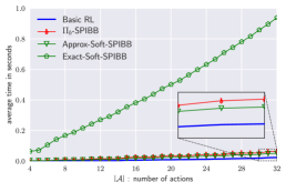
Figure 1: Average time to convergence.

Complexity empirical analysis:

In Figure 1, we show an empirical confirmation of the complexity results on the gridworld task. Exact-Soft-SPIBB has a linear dependency in the number of actions. We also notice that Approx-Soft-SPIBB runs much faster: even faster than $\Pi_{b}$-SPIBB, and 2 times slower than basic RL. Note that the policy improvement step is by design exactly linearly dependent on the number of states $|\mathcal{X}|$. This is the reason why we do not report experiments on the dependency on $|\mathcal{X}|$. We do not report complexity empirical analysis of the other competitors because we do not pretend to have optimal implementations of them, and the purpose of this analysis is to show that Approx-Soft-SPIBB solves the tractability issues of Exact-Soft-SPIBB. In Theory, Robust MDPs and HCPI are more complex by at least an order of magnitude.

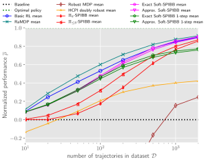
(a) Mean: $\eta=0.9$, $\epsilon=2$

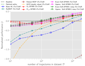
(b) 1%-CVAR: $\eta=0.9$, $\epsilon=2$

Figure 2: Benchmark on Random MDPs domain: mean and 1%-CVAR performances for a hard scenario ($\eta=0.9$) and Soft-SPIBB with $\epsilon=2$

Benchmark results:

Figures 2a and 2b respectively report the mean and 1%-CVAR performances with a strong baseline ($\eta=0.9$). Robust MDPs and HCPI perform poorly and are not further discussed. Basic RL and RaMDP win the benchmark in mean, but fail to do it safely, contrary to Soft-SPIBB and SPIBB algorithms. Exact-Soft-SPIBB is slightly better than Approx-Soft-SPIBB in mean, but also slightly worse in safety. Still in comparison to Approx-Soft-SPIBB, Exact-Soft-SPIBB’s performance does not justify the computational complexity increase and will not be further discussed. Approx-Soft-SPIBB demonstrates a significant improvement over SPIBB methods, both in mean and in safety. Finally, the comparison of Approx-Soft-SPIBB with Approx-Soft-SPIBB 1-step shows that the safety is not improved in practice, and that the asymptotic optimality is compromised when the dataset becomes larger.

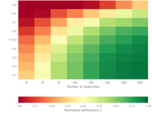
(a) 0.1%-CVaR: RaMDP

(b) 0.1%-CVaR: Approx-Soft-SPIBB, $\epsilon=2$

Figure 3: Influence of $\eta$ on Random MDPs domain: 0.1%-CVaR heatmaps as a function of $\eta$

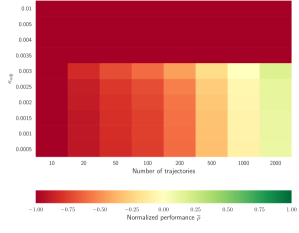
(a) 1%-CVaR: RaMDP, $\eta=0.9$

(b) 1%-CVaR: Approx-Soft-SPIBB, $\eta=0.9$

Figure 4: Sensitivity to hyperparameter on Random MDPs: 1%-CVaR heatmaps for $\eta=0.9$

Sensitivity to the baseline:

We continue the analysis with a heatmap representation as a function of the strength of the baseline: Figures 3a and 3b display heatmaps of the 0.1%-CVaR performance for RaMDP and Approx-Soft-SPIBB ($\epsilon=2$) respectively. The colour of a cell indicates the improvement over the baseline normalized with respect to the optimal performance: red, yellow, and green respectively mean below, equal to, and above baseline performance. We observe that RaMDP is unsafe for strong baselines (high $\eta$ values) and small datasets, while Soft-SPIBB methods become slightly unsafe only with $\eta=0.9$ and less than 20 trajectories, but are safe everywhere else.

Sensitivity to hyper-parameters:

We carry on with 1%-CVaR performance heatmaps as a function of the hyper-parameters for RaMDP (Figure 4a) and Approx-Soft-SPIBB (Figure 4b) in the hardest scenario ($\eta=0.9$). The choice of 1%-CVaR instead of 0.1%-CVaR is justified by the fact that the 0.1%-CVaR RaMDP heatmap is almost completely red, which would not allow us to notice the interesting thresholding behaviour: when $\kappa_{adj}\geq 0.0035$, RaMDP becomes over-conservative to the point of not trying to reach the goal anymore. In contrast, Approx-Soft-SPIBB behaves more smoothly with respect to its hyper-parameter, its optimal value being in interval [0.5,2], depending on the safety/performance trade-off one wants to achieve. In the appendix, Section 0.B.3, the interested reader may find the corresponding heatmaps for all Soft-SPIBB algorithms for mean and 1%-CVaR performances. In particular, we may observe that, despite not having as strong theoretical guarantees as their 1-step versions, the Soft-SPIBB algorithms demonstrate similar CVaR performances.

4.2 Helicopter domain

To assess our algorithms on tasks with more complex state spaces, making the use of function approximation inevitable, we apply them to a helicopter navigation task (Figure LABEL:sub@fig:helicopter). The helicopter’s start point is randomly picked in the teal region, its initial velocity is random as well. The agent can choose to apply or not a fixed amount of thrust forward and backward in the two dimensions, resulting in 9 actions total. An episode ends when the agent reaches the boundary of the blue box or has a speed larger than some maximal value. In the first case, it receives a reward based on its position with respect to the top right corner of the box (the exact reward value is chromatically indicated in the figure). In the second, it gets a reward of $-1$. The dynamics of the helicopter obey Newton’s second law with an additive centered Gaussian noise applied to its position and velocity. We refer the reader to the appendix, Section 0.C.1 for the detailed specifications. We generated a baseline by training online a DQN (Mnih et al.,, 2015) and applying a softmax on the learnt $Q$-network. During training, a discount factor of $0.9$ is used, but the reported results show the undiscounted return obtained by the agent.

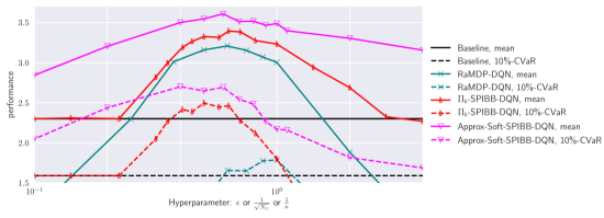
(a) Helicopter benchmark with $|\mathcal{D}|=10,000$

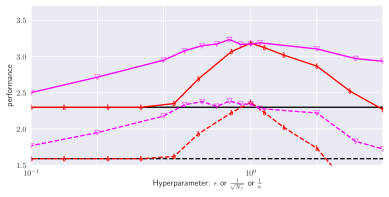
(b) Helicopter benchmark with $|\mathcal{D}|=3,000$

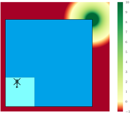
(c) Helicopter domain

Figure 5: Helicopter: mean and 10%-CVaR as a function of the hyper-parameter value

The experiments consist in 300 training runs (necessary to obtain reasonable estimates of algorithms’ safety, the full training procedure is described in the appendix, Section 0.C.3) of RaMDP-DQN, SPIBB-DQN and Approx-Soft-SPIBB-DQN, for different values of their hyper-parameters (resp. $\kappa$, $N_{\wedge}$ and $\epsilon$). We note that for $\kappa=0$, $N_{\wedge}=0$ or $\epsilon=+\infty$, those three algorithms become standard DQN, and that for $N_{\wedge}=\infty$ or $\epsilon=0$, the SPIBB and Soft-SPIBB algorithms produce a copy of the baseline. The three algorithms rely on some estimates of the state-action counts. In this work, we used a pseudo-count estimate heuristic based on Euclidean distance, also detailed in Section 0.C.3. For scalability, we may consider several pseudo-count methodologies from the literature Bellemare et al., (2016); Fox et al., (2018). This is left for future work.

The results of our evaluation can be found in Figure 5, where we plot the mean and 10%-CVaR performances of the different algorithms for two sizes of datasets (more results may be found in the appendix, Section 0.C.4). In order to provide meaningful comparisons, the abscissa represents the different hyper-parameters transformed to account for their dimensional homogeneity (except for a scaling factor). Both Approx-Soft-SPIBB-DQN and SPIBB-DQN outperform RaMDP-DQN by a large margin on the datasets of size 10,000. On the smaller datasets, RaMDP-DQN performs very poorly and does not even appear on the graph. For the same reason, vanilla DQN (mean: 0.22 and 10%-CVaR: -1 with $|\mathcal{D}|=10,000$) does not appear on any of the graphs. The two SPIBB algorithms significantly outperform the baseline both in mean and 10%-CVaR. At their best hyper-parameter value, their 10%-CVaR is actually better than the mean performance of the baseline. Approx-Soft-SPIBB-DQN performs better than SPIBB-DQN both in mean and 10%-CVaR performances. Finally, it is less sensitive than SPIBB-DQN with respect to their respective hyperparameters, and demonstrates a better stability over different dataset sizes. That stability is a useful property as it reduces the requirement for hyper-parameter optimization, which is crucial for Batch RL.

5 Conclusion

We study the problem of safe policy improvement in a Batch RL setting. Building on the SPIBB methodology, we relax the constraints of the policy search to propose a family of algorithms coined Soft-SPIBB. We provide proofs of safety and of computational efficiency for an algorithm called Approx-Soft-SPIBB based on the search of an approximate solution that does not compromise the safety guarantees. We support the theoretical work with an extensive empirical analysis where Approx-Soft-SPIBB shines as the best compromise average performance vs. safety. We further develop Soft-SPIBB in a model-free manner which helps its application to function approximation. Despite the lack of theoretical safety guarantees with function approximation, we observe in our experiments where the function approximation is modelled as a neural network, that Soft-SPIBB allows safe policy improvement in practice and significantly outperforms the competing algorithms both in safety and in performance.

Appendix 0.A Proofs

0.A.1 Preliminaries

We start by recalling the various definitions used in the proofs.

Definition 1

A policy $\pi$ is said to be a policy improvement over a baseline policy $\pi_{b}$ in an MDP $M=\langle\mathcal{X},\mathcal{A},P,R,\gamma\rangle$ if the following inequality holds in every state $x\in\mathcal{X}$:

$$V^{\pi}_{M}(x)\geq V^{\pi_{b}}_{M}(x)$$ (20)

Definition 2

A policy $\pi$ is said to be $\pi_{b}$-advantageous in an MDP $M=\langle\mathcal{X},\mathcal{A},P,R,\gamma\rangle$ if the following inequality holds in every state $x\in\mathcal{X}$:

$$\sum_{a\in\mathcal{A}}A^{\pi_{b}}_{M}(x,a)\pi(a|x)\geq 0$$ (21)

where $A^{\pi_{b}}_{M}(x,a)=Q^{\pi_{b}}_{M}(x,a)-V^{\pi_{b}}_{M}(x)$ quantifies the advantage (or disadvantage) of taking action $a$ in state $x$ instead of following policy $\pi_{b}$.

Definition 3

A policy $\pi$ is said to be $(\pi_{b},e,\epsilon)$-constrained for baseline policy $\pi_{b}$, error function $e$, and a hyper-parameter $\epsilon$ if, for all states $x\in\mathcal{X}$, the following inequality holds:

$$\sum_{a\in\mathcal{A}}e(x,a)\big{\lvert}\pi(a|x)-\pi_{b}(a|x)\big{\rvert}\leq\epsilon.$$

0.A.2 Error Bounds

The difference between an estimated parameter and the true one can be bounded using concentration bounds (or equivalently, Hoeffding’s inequality) applied to the state-action counts in $\mathcal{D}$ (Petrik et al.,, 2016; Laroche et al.,, 2019). Specifically, the following inequalities hold with probability at least $1-\delta$ for any state-action pair $(x,a)\in\mathcal{X}\times\mathcal{A}$:

$$||P^{*}(\cdot|x,a)-\widehat{P}(\cdot|x,a)||_{1} \leq e_{P}(x,a)$$ (22)

$$|R^{*}(x,a)-\widehat{R}(x,a)| \leq e_{P}(x,a)R_{max}$$ (23)

$$\big{\lvert}Q^{\pi_{b}}_{M^{*}}(x,a)-Q^{\pi_{b}}_{\widehat{M}}(x,a)\big{\rvert} \leq e_{Q}(x,a)V_{max}$$ (24)

where:

$$e_{P}(x,a) :=\sqrt{\cfrac{2}{N_{\mathcal{D}}(x,a)}\log\cfrac{2|\mathcal{X}||\mathcal{A}|2^{|\mathcal{X}|}}{\delta}}$$ (25)

$$e_{Q}(x,a) :=\sqrt{\cfrac{2}{N_{\mathcal{D}}(x,a)}\log\cfrac{2|\mathcal{X}||\mathcal{A}|}{\delta}}.$$ (26)

Proof

The three inequalities can be proved similarly to (Petrik et al.,, 2016, Proposition 9). We only detail the proof for (24): for any $(x,a)\in\mathcal{X}\times\mathcal{A}$, and from the two-sided Hoeffding’s inequality,

$$\mathbb{P}\left(\big{\lvert}Q^{\pi_{b}}_{M^{*}}(x,a)-Q^{\pi_{b}}_{\widehat{M}}(x,a)\big{\rvert}>e_{Q}(x,a)V_{max}\right)$$

$$=\mathbb{P}\left(\frac{\big{\lvert}Q^{\pi_{b}}_{M^{*}}(x,a)-Q^{\pi_{b}}_{\widehat{M}}(x,a)\big{\rvert}}{2V_{max}}>\sqrt{\frac{1}{2N_{\mathcal{D}}(x,a)}\log\frac{2|\mathcal{X}||\mathcal{A}|}{\delta}}\right)$$

$$\leq 2\exp\left(-2N_{\mathcal{D}}(x,a)\frac{1}{2N_{\mathcal{D}}(x,a)}\log\frac{2|\mathcal{X}||\mathcal{A}|}{\delta}\right)$$

$$\leq\frac{\delta}{|\mathcal{X}||\mathcal{A}|}$$

By summing all $|\mathcal{X}||\mathcal{A}|$ state-action pairs error probabilities lower than $\frac{\delta}{|\mathcal{X}||\mathcal{A}|}$, we obtain (24).

0.A.3 Proof of Theorem 3.1

In this section, we prove Theorem 3.1:

Theorem 0.A.1

Any $(\pi_{b},e_{Q},\epsilon)$-constrained policy $\pi$ that is $\pi_{b}$-advantageous in $\widehat{M}$ satisfies the following inequality in every state $x$ with probability at least $1-\delta$:

$$V^{\pi}_{M^{*}}(x)-V^{\pi_{b}}_{M^{*}}(x) \geq-\cfrac{\epsilon V_{max}}{1-\gamma}.$$ (27)

Proof

We start from Proposition 38 with $M=M^{*}$, $\pi_{1}=\pi$, and $\pi_{2}=\pi_{b}$:

$$V^{\pi}_{M^{*}}-V^{\pi_{b}}_{M^{*}} =Q^{\pi_{b}}_{M^{*}}\left(\pi-\pi_{b}\right)d_{M^{*}}^{\pi}$$ (28)

$$=\left(Q^{\pi_{b}}_{M^{*}}-Q^{\pi_{b}}_{\widehat{M}}+Q^{\pi_{b}}_{\widehat{M}}\right)\left(\pi-\pi_{b}\right)d_{M^{*}}^{\pi}$$ (29)

$$=\left(Q^{\pi_{b}}_{M^{*}}-Q^{\pi_{b}}_{\widehat{M}}\right)\left(\pi-\pi_{b}\right)d_{M^{*}}^{\pi}+Q^{\pi_{b}}_{\widehat{M}}\left(\pi-\pi_{b}\right)d_{M^{*}}^{\pi}.$$ (30)

The first term is bounded by $\frac{\epsilon V_{max}}{1-\gamma}$ thanks to inequality 26, the $(\pi_{b},e_{Q},\epsilon)$-constrained policy property and Holder’s inequality:

$$\Big{\lVert} \left(Q^{\pi_{b}}_{M^{*}}-Q^{\pi_{b}}_{\widehat{M}}\right)\left(\pi-\pi_{b}\right)d_{M^{*}}^{\pi}\Big{\rVert}_{\infty}\leq\Big{\lVert}\left(Q^{\pi_{b}}_{M^{*}}-Q^{\pi_{b}}_{\widehat{M}}\right)\left(\pi-\pi_{b}\right)\Big{\rVert}_{\infty}\big{\lVert}d_{M^{*}}^{\pi}\big{\rVert}_{1}$$ (31)

$$\leq\max_{x}\sum_{a}(Q^{\pi_{b}}_{M^{*}}(x,a)-Q^{\pi_{b}}_{\widehat{M}}(x,a))\left(\pi(a|x)-\pi_{b}(a|x)\right)\cfrac{1}{1-\gamma}$$ (32)

$$\leq\cfrac{\epsilon V_{max}}{1-\gamma}.$$ (33)

Let us now prove that the second term of Equation 30 is positive. It is the product of vector $Q^{\pi_{b}}_{\widehat{M}}\left(\pi-\pi_{b}\right)$ with matrix $d_{M^{*}}^{\pi}$. All the terms of $d_{M^{*}}^{\pi}$ are positive so it suffices to show that each element of the vector is positive. We have for each $x\in\mathcal{X}$:

$$\left(Q^{\pi_{b}}_{\widehat{M}}\left(\pi-\pi_{b}\right)\right)(x) =\sum_{a}Q^{\pi_{b}}_{\widehat{M}}(x,a)\left(\pi(a|x)-\pi_{b}(a|x)\right)$$ (34)

$$=\sum_{a}Q^{\pi_{b}}_{\widehat{M}}(x,a)\pi(a|x)-V^{\pi_{b}}_{\widehat{M}}(x)$$ (35)

$$=\sum_{a\in\mathcal{A}}A^{\pi_{b}}_{M}(x,a)\pi(a|x)\geq 0$$ (36)

where the last inequality comes from $\pi$ being $\pi_{b}$-advantageous in $\widehat{M}$. This concludes the proof.  $\square$

0.A.4 Proof of Theorem 3.2

In this section, we prove Theorem 3.2 from the main text. Let us start with:

Proposition 1

Let $M=\langle\mathcal{X},\mathcal{A},P,R,\gamma\rangle$ be an MDP, and $\pi_{1}$ and $\pi_{2}$ be two policies defined on this MDP. We have:

$$V^{\pi_{1}}_{M}-V^{\pi_{2}}_{M}=Q^{\pi_{1}}_{M}\left(\pi_{1}-\pi_{2}\right)d_{M}^{\pi_{2}}=Q^{\pi_{2}}_{M}\left(\pi_{1}-\pi_{2}\right)d_{M}^{\pi_{1}},$$ (37)

where $d_{M}^{\pi}$ is a matrix that assigns to element $d_{M}^{\pi}(x^{\prime}|x)$ the expectation of the discounted sum of visits to state $x^{\prime}$, starting from $x$, and when following policy $\pi$ in MDP $M$ (it is actually only dependent on the transition dynamics $P$). Formally, it is written as:

$$d_{M}^{\pi}(x^{\prime}|x)=\sum_{t=0}^{\infty}\gamma^{t}\mathbb{P}(X_{t}=x^{\prime}|X_{t}\sim P\pi X_{t-1},X_{0}=x)$$ (38)

Proof

$$V^{\pi_{1}}_{M}-V^{\pi_{2}}_{M} =(R+\gamma V^{\pi_{1}}_{M}P)\pi_{1}-(R+\gamma V^{\pi_{2}}_{M}P)\pi_{2}$$ (39)

$$=(R+\gamma V^{\pi_{1}}_{M}P)(\pi_{1}-\pi_{2})+\gamma(V^{\pi_{1}}_{M}-V^{\pi_{2}}_{M})P\pi_{2}$$ (40)

$$=Q^{\pi_{1}}_{M}(\pi_{1}-\pi_{2})+\gamma(V^{\pi_{1}}_{M}-V^{\pi_{2}}_{M})P\pi_{2}$$ (41)

$$\left(V^{\pi_{1}}_{M}-V^{\pi_{2}}_{M}\right)\left(\mathbb{I}-\gamma P\pi_{2}\right) =Q^{\pi_{1}}_{M}(\pi_{1}-\pi_{2})$$ (42)

$$V^{\pi_{1}}_{M}-V^{\pi_{2}}_{M} =Q^{\pi_{1}}_{M}(\pi_{1}-\pi_{2})\left(\mathbb{I}-\gamma P\pi_{2}\right)^{-1}$$ (43)

The last line is obtained because $P\pi_{2}$ is a stochastic matrix and $0\leq\gamma<1$. As a result, $\mathbb{I}-\gamma P\pi_{2}$ is invertible and is indeed the state distribution matrix $d_{M}^{\pi_{2}}$. The other equality: $V^{\pi_{1}}_{M}-V^{\pi_{2}}_{M}=Q^{\pi_{2}}_{M}(\pi_{1}-\pi_{2})d_{M}^{\pi_{1}}$ is obtained in a symmetrical way.  $\square$

Proposition 2

Let $M_{1}$ and $M_{2}$ be two MDPs: $M_{1}=\langle\mathcal{X},\mathcal{A},P_{1},R_{1},\gamma\rangle$ and $M_{2}=\langle\mathcal{X},\mathcal{A},P_{2},R_{2},\gamma\rangle$. Let $\pi_{1},\pi_{2}$ be two policies defined on these MDPs, then:

$$V^{\pi_{1}}_{M_{1}}-V^{\pi_{2}}_{M_{1}}=V^{\pi_{1}}_{M_{2}}-V^{\pi_{2}}_{M_{2}} +Q^{\pi}_{M_{2}}\left(\pi_{1}-\pi_{2}\right)\left(d_{M_{1}}^{\pi_{2}}-d_{M_{2}}^{\pi_{2}}\right)$$ (44)

$$+\left(Q^{\pi}_{M_{1}}-Q^{\pi}_{M_{2}}\right)\left(\pi_{1}-\pi_{2}\right)d_{M_{1}}^{\pi_{2}}$$ (45)

Proof

From Proposition 38:

$$V^{\pi_{1}}_{M_{1}}-V^{\pi_{2}}_{M_{1}} =Q^{\pi_{1}}_{M_{1}}\left(\pi_{1}-\pi_{2}\right)d_{M_{1}}^{\pi_{2}}$$ (46)

$$=\left(Q^{\pi_{1}}_{M_{2}}+Q^{\pi_{1}}_{M_{1}}-Q^{\pi_{1}}_{M_{2}}\right)\left(\pi_{1}-\pi_{2}\right)d_{M_{1}}^{\pi_{2}}$$ (47)

$$=Q^{\pi_{1}}_{M_{2}}\left(\pi_{1}-\pi_{2}\right)d_{M_{1}}^{\pi_{2}}+\left(Q^{\pi_{1}}_{M_{1}}-Q^{\pi_{1}}_{M_{2}}\right)\left(\pi_{1}-\pi_{2}\right)d_{M_{1}}^{\pi_{2}}$$ (48)

$$=Q^{\pi_{1}}_{M_{2}}\left(\pi_{1}-\pi_{2}\right)\left(d_{M_{2}}^{\pi_{2}}+d_{M_{1}}^{\pi_{2}}-d_{M_{2}}^{\pi_{2}}\right)+\left(Q^{\pi_{1}}_{M_{1}}-Q^{\pi_{1}}_{M_{2}}\right)\left(\pi_{1}-\pi_{2}\right)d_{M_{1}}^{\pi_{2}}$$ (49)

$$=Q^{\pi_{1}}_{M_{2}}\left(\pi_{1}-\pi_{2}\right)d_{M_{2}}^{\pi_{2}}+Q^{\pi_{1}}_{M_{2}}\left(\pi_{1}-\pi_{2}\right)\left(d_{M_{1}}^{\pi_{2}}-d_{M_{2}}^{\pi_{2}}\right)$$ (50)

$$\quad\quad\quad\quad\quad\quad\quad\quad\quad\;\>+\left(Q^{\pi_{1}}_{M_{1}}-Q^{\pi_{1}}_{M_{2}}\right)\left(\pi_{1}-\pi_{2}\right)d_{M_{1}}^{\pi_{2}}$$ (51)

The first term of Equation 51 is transformed by applying Proposition 38 to $M_{2}$:

$$Q^{\pi_{1}}_{M_{2}}\left(\pi_{1}-\pi_{2}\right)d_{M_{2}}^{\pi_{2}}=V^{\pi_{1}}_{M_{2}}-V^{\pi_{2}}_{M_{2}},$$ (52)

which concludes the proof.  $\square$

The proof of the theorem requires the following assumption (see the main text for a discussion on it):

Assumption 1

There exists a constant $\kappa<\frac{1}{\gamma}$ such that, for all state-action pairs $(x,a)\in\mathcal{X}\times\mathcal{A}$ the following inequality holds:

$$\sum_{x^{\prime},a^{\prime}}e_{P}(x^{\prime},a^{\prime})\pi_{b}(a^{\prime}|x^{\prime})P^{*}(x^{\prime}|x,a)\leq\kappa e(x,a)$$ (53)

That assumption allows to prove Lemma 1:

Lemma 1

Under Assumption 1, any $(\pi_{b},e_{P},\epsilon)$-constrained policy $\pi$ satisfies the following inequality for every state-action pair $(x,a)$ with probability at least $1-\delta$:

$$\big{\lvert}Q^{\pi}_{M^{*}}(x,a)-Q^{\pi}_{\widehat{M}}(x,a)\big{\rvert}\leq\left(\cfrac{e_{P}(x,a)}{1-\kappa\gamma}+\cfrac{\gamma\epsilon}{\left(1-\gamma\right)\left(1-\kappa\gamma\right)}\right)V_{max}.$$

Proof sketch

Let $Q^{*}_{0}=0$, $\widehat{Q}_{0}=0$, $Q^{*}_{t+1}=\mathcal{B}^{*}(Q^{*}_{t})$ and $\widehat{Q}_{t+1}=\widehat{\mathcal{B}}(\widehat{Q}_{t})$, where $\mathcal{B}^{*}$ and $\widehat{\mathcal{B}}$ denote the Bellman operators for policy $\pi$ in the true and estimated MDP. We proceed by induction to prove inequality 1 on $\lvert Q^{*}_{t}(x,a)-\widehat{Q}_{t}(x,a)\lvert$:

$$Q^{*}_{t+1}(x,a)-\widehat{Q}_{t+1}(x,a) =R^{*}(x,a)-\widehat{R}(x,a)$$ (54)

$$+\sum_{x^{\prime},a^{\prime}}\gamma\left(Q^{*}_{t}(x^{\prime},a^{\prime})-\widehat{Q}_{t}(x^{\prime},a^{\prime})\right)\pi(a^{\prime}|x^{\prime})P^{*}(x^{\prime}|x,a)$$

$$+\sum_{x^{\prime},a^{\prime}}\gamma\widehat{Q}_{t}(x^{\prime},a^{\prime})\pi(a^{\prime}|x^{\prime})\left(P^{*}(x^{\prime}|x,a)-\widehat{P}(x^{\prime}|x,a)\right).$$

By applying the inductive hypothesis and inequality 1 (which holds true with probability at least $1-\delta$):

$$\big{\lvert}Q^{*}_{t+1}(x,a)-\widehat{Q}_{t+1}(x,a)\big{\rvert} \leq e_{P}(x,a)V_{max}+\cfrac{\gamma^{2}\epsilon V_{max}}{\left(1-\gamma\right)\left(1-\kappa\gamma\right)}$$

$$+\sum_{x^{\prime},a^{\prime}}\cfrac{\gamma e_{P}(x^{\prime},a^{\prime})}{1-\kappa\gamma}\pi_{b}(a^{\prime}|x^{\prime})P^{*}(x^{\prime}|x,a)V_{max}$$ (55)

$$+\sum_{x^{\prime},a^{\prime}}\cfrac{\gamma e_{P}(x^{\prime},a^{\prime})}{1-\kappa\gamma}\lvert\pi(a^{\prime}|x^{\prime})-\pi_{b}(a^{\prime}|x^{\prime})\rvert P^{*}(x^{\prime}|x,a)V_{max}.$$

The $(\pi_{b},e_{P},\epsilon)$-constrained property of $\pi$ ensures that

$$\forall x^{\prime}\in\mathcal{X},\ {\sum_{a^{\prime}}e_{P}(x^{\prime},a^{\prime})\lvert\pi(a^{\prime}|x^{\prime})-\pi_{b}(a^{\prime}|x^{\prime})\rvert\leq\epsilon}$$

Applying Assumption 1 and some algebraic manipulations allows to conclude the induction. Taking the limit proves the lemma since $(Q^{*}_{t},\widehat{Q}_{t})\rightarrow(Q^{\pi}_{M^{*}},Q^{\pi}_{\widehat{M}})$.  $\square$

Proof

We let $\mathcal{B}^{*}$ and $\widehat{\mathcal{B}}$ denote the Bellman operators for policy $\pi$ in the true and estimated MDP. We have e.g.:

$$\mathcal{B}^{*}(Q)(x,a) =R^{*}(x,a)+\sum_{x^{\prime},a^{\prime}}\gamma Q(x^{\prime},a^{\prime})\pi(a^{\prime}|x^{\prime})P^{*}(x^{\prime}|x,a).$$

We now proceed by induction. Let $Q^{*}_{0}=0$, $\widehat{Q}_{0}=0$, $Q^{*}_{t+1}=\mathcal{B}^{*}(Q^{*}_{t})$ and $\widehat{Q}_{t+1}=\widehat{\mathcal{B}}(\widehat{Q}_{t})$. We wish to prove that :

$$\lvert Q^{*}_{t}(x,a)-\widehat{Q}_{t}(x,a)\rvert\leq\left(\cfrac{e_{P}(x,a)}{1-\kappa\gamma}+\cfrac{\gamma\epsilon}{\left(1-\gamma\right)\left(1-\kappa\gamma\right)}\right)V_{max}.$$

By definition we have:

$$Q^{*}_{t+1}(x,a)-\widehat{Q}_{t+1}(x,a) =\mathcal{B}^{*}(Q^{*}_{t})(x,a)-\widehat{\mathcal{B}}(\widehat{Q}_{t})(x,a)$$ (56)

$$=R^{*}(x,a)-\widehat{R}(x,a)+\sum_{x^{\prime},a^{\prime}}\gamma Q^{*}_{t}(x^{\prime},a^{\prime})\pi(a^{\prime}|x^{\prime})P^{*}(x^{\prime}|x,a)$$

$$\quad\quad\quad\quad\quad-\sum_{x^{\prime},a^{\prime}}\gamma\widehat{Q}_{t}(x^{\prime},a^{\prime})\pi(a^{\prime}|x^{\prime})\widehat{P}(x^{\prime}|x,a)$$ (57)

$$=R^{*}(x,a)-\widehat{R}(x,a)$$

$$\quad\quad+\sum_{x^{\prime},a^{\prime}}\gamma\left(Q^{*}_{t}(x^{\prime},a^{\prime})-\widehat{Q}_{t}(x^{\prime},a^{\prime})\right)\pi(a^{\prime}|x^{\prime})P^{*}(x^{\prime}|x,a)$$

$$\quad\quad+\sum_{x^{\prime},a^{\prime}}\gamma\widehat{Q}_{t}(x^{\prime},a^{\prime})\pi(a^{\prime}|x^{\prime})\left(P^{*}(x^{\prime}|x,a)-\widehat{P}(x^{\prime}|x,a)\right)$$ (58)

We apply inequality 23 to the first term, the inductive hypothesis at time $t$ to the second and inequality 22 and Holder’s inequality to the third to get:

$$\lvert Q^{*}_{t+1} (x,a)-\widehat{Q}_{t+1}(x,a)\rvert$$

$$\leq e_{P}(x,a)R_{max}+\gamma e_{P}(x,a)V_{max}$$

$$\quad+\sum_{x^{\prime},a^{\prime}}\gamma\left(\cfrac{e_{P}(x^{\prime},a^{\prime})}{1-\kappa\gamma}+\cfrac{\gamma\epsilon}{\left(1-\gamma\right)\left(1-\kappa\gamma\right)}\right)\pi(a^{\prime}|x^{\prime})P^{*}(x^{\prime}|x,a)V_{max}$$ (59)

$$=e_{P}(x,a)V_{max}+\cfrac{\gamma^{2}\epsilon V_{max}}{\left(1-\gamma\right)\left(1-\kappa\gamma\right)}$$

$$\quad+\sum_{x^{\prime},a^{\prime}}\cfrac{\gamma e_{P}(x^{\prime},a^{\prime})}{1-\kappa\gamma}\pi(a^{\prime}|x^{\prime})P^{*}(x^{\prime}|x,a)V_{max}$$ (60)

$$=e_{P}(x,a)V_{max}+\cfrac{\gamma^{2}\epsilon V_{max}}{\left(1-\gamma\right)\left(1-\kappa\gamma\right)}$$

$$\quad+\sum_{x^{\prime},a^{\prime}}\cfrac{\gamma e_{P}(x^{\prime},a^{\prime})}{1-\kappa\gamma}\left(\pi(a^{\prime}|x^{\prime})-\pi_{b}(a^{\prime}|x^{\prime})+\pi_{b}(a^{\prime}|x^{\prime})\right)P^{*}(x^{\prime}|x,a)V_{max}$$ (61)

$$\leq e_{P}(x,a)V_{max}+\cfrac{\gamma^{2}\epsilon V_{max}}{\left(1-\gamma\right)\left(1-\kappa\gamma\right)}$$

$$\quad+\sum_{x^{\prime},a^{\prime}}\cfrac{\gamma e_{P}(x^{\prime},a^{\prime})}{1-\kappa\gamma}\pi_{b}(a^{\prime}|x^{\prime})P^{*}(x^{\prime}|x,a)V_{max}$$

$$\quad+\sum_{x^{\prime},a^{\prime}}\cfrac{\gamma e_{P}(x^{\prime},a^{\prime})}{1-\kappa\gamma}\lvert\pi(a^{\prime}|x^{\prime})-\pi_{b}(a^{\prime}|x^{\prime})\rvert P^{*}(x^{\prime}|x,a)V_{max}$$ (62)

By the $(\pi_{b},e_{P},\epsilon)$-constrained property, we know that $\forall x^{\prime},\sum_{a^{\prime}}e_{P}(x^{\prime},a^{\prime})\lvert\pi(a^{\prime}|x^{\prime})-\pi_{b}(a^{\prime}|x^{\prime})\rvert\leq\epsilon$. Applying Holder’s inequality and combining the second and fourth term, we find:

$$\lvert Q^{*}_{t+1}(x,a)-\widehat{Q}_{t+1}(x,a)\rvert \leq e_{P}(x,a)V_{max}+\cfrac{\gamma\epsilon V_{max}}{\left(1-\gamma\right)\left(1-\kappa\gamma\right)}$$

$$\quad+\sum_{x^{\prime},a^{\prime}}\cfrac{\gamma e_{P}(x^{\prime},a^{\prime})}{1-\kappa\gamma}\pi_{b}(a^{\prime}|x^{\prime})P^{*}(x^{\prime}|x,a)V_{max}$$ (63)

By Assumption 1, we know that $\forall x,\sum_{x^{\prime},a^{\prime}}e_{P}(x^{\prime},a^{\prime})\pi_{b}(a^{\prime}|x^{\prime})P^{*}(x^{\prime}|x,a)\leq\kappa e_{P}(x,a)$. This gives:

$$\lvert Q^{*}_{t+1}(x,a)-\widehat{Q}_{t+1}(x,a)\rvert \leq e_{P}(x,a)V_{max}+\cfrac{\gamma\epsilon V_{max}}{\left(1-\gamma\right)\left(1-\kappa\gamma\right)}+\cfrac{\kappa\gamma e_{P}(x,a)}{1-\kappa\gamma}V_{max}$$ (64)

$$=\cfrac{e_{P}(x,a)V_{max}}{1-\kappa\gamma}+\cfrac{\gamma\epsilon V_{max}}{\left(1-\gamma\right)\left(1-\kappa\gamma\right)}$$ (65)

$$=\left(\cfrac{e_{P}(x,a)}{1-\kappa\gamma}+\cfrac{\gamma\epsilon}{\left(1-\gamma\right)\left(1-\kappa\gamma\right)}\right)V_{max},$$ (66)

which concludes the induction. From standard properties of the Bellman operator, taking the limit proves the lemma.  $\square$

Theorem 0.A.2

Under Assumption 1, any $(\pi_{b},e_{P},\epsilon)$-constrained policy $\pi$ satisfies the following inequality in every state $x$ with probability at least $1-\delta$:

$$V^{\pi}_{M^{*}}(x)-V^{\pi_{b}}_{M^{*}}(x)\geq V^{\pi}_{\widehat{M}}(x)-V^{\pi_{b}}_{\widehat{M}}(x) -2\big{\lVert}d^{\pi_{b}}_{M^{*}}(\,\boldsymbol{\cdot}\,|x)-d^{\pi_{b}}_{\widehat{M}}(\,\boldsymbol{\cdot}\,|x)\big{\rVert}_{1}V_{max}$$

$$-\cfrac{1+\gamma}{\left(1-\gamma\right)^{2}\left(1-\kappa\gamma\right)}\;\;\epsilon V_{max}.$$ (67)

Proof sketch

We first prove the following:

$$V^{\pi}_{M^{*}}-V^{\pi_{b}}_{M^{*}}=V^{\pi}_{\widehat{M}}-V^{\pi_{b}}_{\widehat{M}} +Q^{\pi}_{\widehat{M}}\left(\pi-\pi_{b}\right)\left(d_{M^{*}}^{\pi_{b}}-d_{\widehat{M}}^{\pi_{b}}\right)$$

$$+\left(Q^{\pi}_{M^{*}}-Q^{\pi}_{\widehat{M}}\right)\left(\pi-\pi_{b}\right)d_{M^{*}}^{\pi_{b}}.$$ (68)

We then apply Holder’s inequality twice to the second term:

$$\Big{\lVert}Q^{\pi}_{\widehat{M}}\left(\pi-\pi_{b}\right)\left(d^{\pi_{b}}_{M^{*}}-d^{\pi_{b}}_{\widehat{M}}\right)(\,\boldsymbol{\cdot}\,|x)\Big{\rVert}_{1}\leq 2\Big{\lVert}\left(d^{\pi_{b}}_{M^{*}}-d^{\pi_{b}}_{\widehat{M}}\right)(\,\boldsymbol{\cdot}\,|x)\Big{\rVert}_{1}V_{max}.$$ (69)

Afterwards, thanks to Assumption 1, we may use Lemma 1 to bound the third term in function of $V_{max},\epsilon,\gamma$, and $\kappa$:

$$\Big{\lVert}\left(Q^{\pi}_{M^{*}}-Q^{\pi}_{\widehat{M}}\right)\left(\pi-\pi_{b}\right)d^{\pi_{b}}_{M^{*}}(\,\boldsymbol{\cdot}\,|x)\Big{\rVert}_{1}\leq\cfrac{1+\gamma}{\left(1-\gamma\right)^{2}\left(1-\kappa\gamma\right)}\;\;\epsilon V_{max}.$$ (70)

Plugging all the pieces together proves the theorem.  $\square$

Proof

We first apply Proposition 2 with $M_{1}=M^{*},M_{2}=\widehat{M},\pi_{1}=\pi$, and $\pi_{2}=\pi_{b}$:

$$V^{\pi}_{M^{*}}-V^{\pi_{b}}_{M^{*}} =V^{\pi}_{\widehat{M}}-V^{\pi_{b}}_{\widehat{M}}+Q^{\pi}_{\widehat{M}}\left(\pi-\pi_{b}\right)\left(d_{M^{*}}^{\pi_{b}}-d_{\widehat{M}}^{\pi_{b}}\right)$$

$$\quad+\left(Q^{\pi}_{M^{*}}-Q^{\pi}_{\widehat{M}}\right)\left(\pi-\pi_{b}\right)d_{M^{*}}^{\pi_{b}}$$ (71)

$$V^{\pi}_{M^{*}}(x)-V^{\pi_{b}}_{M^{*}}(x) \leq V^{\pi}_{\widehat{M}}(x)-V^{\pi_{b}}_{\widehat{M}}(x)-\Big{\lVert}Q^{\pi}_{\widehat{M}}\left(\pi-\pi_{b}\right)\left(d_{M^{*}}^{\pi_{b}}-d_{\widehat{M}}^{\pi_{b}}\right)(\,\boldsymbol{\cdot}\,|x)\Big{\rVert}_{1}$$

$$\quad-\Big{\lVert}\left(Q^{\pi}_{M^{*}}-Q^{\pi}_{\widehat{M}}\right)\left(\pi-\pi_{b}\right)d^{*}_{\pi_{b}}(\,\boldsymbol{\cdot}\,|x)\Big{\rVert}_{1}.$$ (72)

Then, we apply twice Holder’s inequality to the second term 1-norm:

$$\Big{\lVert}Q^{\pi}_{\widehat{M}}\left(\pi-\pi_{b}\right) \left(d^{\pi_{b}}_{M^{*}}-d^{\pi_{b}}_{\widehat{M}}\right)(\,\boldsymbol{\cdot}\,|x)\Big{\rVert}_{1}$$

$$\leq\big{\lVert}Q^{\pi}_{\widehat{M}}\big{\rVert}_{\infty}\big{\lVert}\left(\pi-\pi_{b}\right)(\,\boldsymbol{\cdot}\,|x^{\prime})\big{\rVert}_{1}\Big{\lVert}\left(d^{\pi_{b}}_{M^{*}}-d^{\pi_{b}}_{\widehat{M}}\right)(\,\boldsymbol{\cdot}\,|x)\Big{\rVert}_{1}$$ (73)

$$\leq 2\Big{\lVert}\left(d^{\pi_{b}}_{M^{*}}-d^{\pi_{b}}_{\widehat{M}}\right)(\,\boldsymbol{\cdot}\,|x)\Big{\rVert}_{1}.V_{max}.$$ (74)

Similarly, we obtain the following with the third term:

$$\Big{\lVert} \left(Q^{\pi}_{M^{*}}-Q^{\pi}_{\widehat{M}}\right)\left(\pi-\pi_{b}\right)d^{*}_{\pi_{b}}(\,\boldsymbol{\cdot}\,|x)\Big{\rVert}_{1}$$

$$\leq\big{\lVert}d^{*}_{\pi_{b}}(\,\boldsymbol{\cdot}\,|x)\big{\rVert}_{1}\max_{x^{\prime}}\sum_{a^{\prime}}\left(Q^{\pi}_{M^{*}}(x^{\prime},a^{\prime})-Q^{\pi}_{\widehat{M}}(x^{\prime},a^{\prime})\right)\left(\pi(a^{\prime}|x^{\prime})-\pi_{b}(a^{\prime}|x^{\prime})\right)$$ (75)

$$\leq\cfrac{1}{1-\gamma}\max_{x^{\prime}}\sum_{a^{\prime}}\big{\lvert}Q^{\pi}_{M^{*}}(x^{\prime},a^{\prime})-Q^{\pi}_{\widehat{M}}(x^{\prime},a^{\prime})\big{\rvert}\lvert\pi(a^{\prime}|x^{\prime})-\pi_{b}(a^{\prime}|x^{\prime})\rvert.$$ (76)

We use Lemma 1 to bound the third term in function of $V_{max},\epsilon,\gamma$, and $e_{P}(x^{\prime},a^{\prime})$:

$$\Big{\lVert} \left(Q^{\pi}_{M^{*}}-Q^{\pi}_{\widehat{M}}\right)\left(\pi-\pi_{b}\right)d^{*}_{\pi_{b}}(\,\boldsymbol{\cdot}\,|x)\Big{\rVert}_{1}$$

$$\leq\cfrac{1}{1-\gamma}\max_{x^{\prime}}\sum_{a^{\prime}}\left(\cfrac{e_{P}(x^{\prime},a^{\prime})}{1-\kappa\gamma}+\cfrac{\gamma\epsilon}{\left(1-\gamma\right)\left(1-\kappa\gamma\right)}\right)V_{max}\lvert\pi(a^{\prime}|x^{\prime})-\pi_{b}(a^{\prime}|x^{\prime})\rvert$$ (77)

$$\leq\cfrac{1}{1-\gamma}\max_{x^{\prime}}\left(\cfrac{\sum_{a^{\prime}}e_{P}(x^{\prime},a^{\prime})\lvert\pi(a^{\prime}|x^{\prime})-\pi_{b}(a^{\prime}|x^{\prime})\rvert}{1-\kappa\gamma}+\cfrac{2\gamma\epsilon}{\left(1-\gamma\right)\left(1-\kappa\gamma\right)}\right)V_{max}$$ (78)

$$\leq\cfrac{1}{1-\gamma}\max_{x^{\prime}}\cfrac{1+\gamma}{\left(1-\gamma\right)\left(1-\kappa\gamma\right)}\;\;\epsilon V_{max}$$ (79)

$$\leq\cfrac{1+\gamma}{\left(1-\gamma\right)^{2}\left(1-\kappa\gamma\right)}\;\;\epsilon V_{max}$$ (80)

where the third line uses the $(\pi_{b},e_{P},\epsilon)$-constrained assumption. Plugging all the pieces together proves the theorem.  $\square$

Proposition 3

Let $M$ be an MDP: $\langle\mathcal{X},\mathcal{A},P,R,\gamma\rangle$, $\pi_{b}$ be the baseline policy on which trajectories $\mathcal{D}$ have been collected, $\widehat{M}$ be the MLE MDP: $\langle\mathcal{X},\mathcal{A},P,R,\gamma\rangle$, and $N_{\mathcal{D}}(x)$ be the count of transitions starting from state $x\in\mathcal{X}$ in $\mathcal{D}$. Then, the following concentration bound holds with high probabilities $1-\delta$:

$$\Big{\lVert}\left(d^{\pi_{b}}_{M}-d^{\pi_{b}}_{\widehat{M}}\right)(\,\boldsymbol{\cdot}\,|x)\Big{\rVert}_{1} \leq\cfrac{1}{1-\gamma}\sqrt{\cfrac{2}{N_{\mathcal{D}}(x)}\log\cfrac{2^{|\mathcal{X}|}}{\delta}}.$$ (81)

Proof

We apply concentration bounds. The proof relies on Theorem 2.1 in Weissman et al., (2003) and is identical to that of Equation 25 borrowed from Petrik et al., (2016), except that $d^{\pi_{b}}_{M}$ and $d^{\pi_{b}}_{\widehat{M}}$ are state distributions and not probability distributions and that their sums are therefore bounded by $\frac{1}{1-\gamma}$. It gives:

$$\Big{\lVert}\left(d^{\pi_{b}}_{M}-d^{\pi_{b}}_{\widehat{M}}\right)(\,\boldsymbol{\cdot}\,|x)\Big{\rVert}_{1} \leq\cfrac{1}{1-\gamma}\sqrt{\cfrac{2}{N_{\mathcal{D}}(x)}\log\cfrac{2^{|\mathcal{X}|}}{\delta}},$$ (82)

which concludes the proof.  $\square$

0.A.5 Proof of Theorem 3.3

Theorem 0.A.3

The policy improvement step of Approx-Soft-SPIBB generates policies that are guaranteed to be $(\pi_{b},e,\epsilon)$-constrained.

Proof

The summation of the product of probability mass moved and the error function is below the budget $\epsilon$ by design.  $\square$

0.A.6 Proof of Theorem 3.4

Theorem 0.A.4

Approx-Soft-SPIBB policy improvement has a complexity of $\mathcal{O}(|\mathcal{X}||\mathcal{A}|^{2})$.

Proof

Approx-Soft-SPIBB performs a loop over the state space $\mathcal{X}$ and within that loop a set of operations over the action space. It sorts once the action space in terms of $Q_{\widehat{M}}^{(i)}$ and for each action performs an $\operatorname*{argmax}$ over $|\mathcal{A}|$. This results in a $|\mathcal{A}|^{2}$ complexity for each state.  $\square$

0.A.7 Proof of Theorem 3.5

Theorem 0.A.5

Considering an MDP with exact counts, the model-based policy iteration of (Exact or Approx)-Soft-SPIBB is identical to the model-free policy iteration of (resp. Exact or Approx)-Soft-SPIBB.

Proof

Let $\pi^{(i+1)}$ be the (exact or approximate) policy improvement, which is assumed to be identical in the model-free and the model-based implementations of Soft-SPIBB. Then, it means that:

$$Q^{(i+1)}_{M\text{-}Based}(x,a) =\widehat{R}(x,a)+\gamma\sum_{x^{\prime}\in\mathcal{X}}\widehat{P}(x^{\prime}|x,a)\sum_{a^{\prime}\in\mathcal{A}}\pi^{(i+1)}(a^{\prime}|x^{\prime})Q^{(i)}(x^{\prime},a^{\prime})$$ (83)

$$=\cfrac{\displaystyle\sum_{\langle x_{j}=x,a_{j}=a,x^{\prime}_{j},r_{j}\rangle\in\mathcal{D}}r_{j}}{N_{\mathcal{D}}(x,a)}$$

$$\quad+\gamma\cfrac{\displaystyle\sum_{\langle x_{j}=x,a_{j}=a,x^{\prime}_{j},r_{j}\rangle\in\mathcal{D}}\>\sum_{a^{\prime}\in\mathcal{A}}\pi^{(i+1)}(a^{\prime}|x^{\prime}_{j})Q^{(i)}(x^{\prime}_{j},a^{\prime})}{N_{\mathcal{D}}(x,a)}$$ (84)

$$=\cfrac{y^{(i)}_{j}}{N_{\mathcal{D}}(x,a)}=Q^{(i+1)}_{M\text{-}Free}(x,a),$$ (85)

where Equation 84 is obtained from the MLE MDP $\widehat{M}=\langle\mathcal{X},\mathcal{A},\widehat{P},\widehat{R},\gamma\rangle$ definition, and Equation 85 is obtained thanks to the target definition from Equation 18.  $\square$

0.A.8 Approximate policy improvement pseudo-code

Input: Baseline policy $\pi_{b}$, current state $x$, action set $\mathcal{A}$, errors $e(x,a)$ for each $a\in\mathcal{A}$, precision level $\epsilon$ and last iteration value function $Q^{(i)}_{\widehat{M}}$

Initialize $\pi^{(i+1)}(\cdot|x)=\pi_{b}(\cdot|x)$ and $E=\epsilon$.

Define $\mathcal{A^{-}}$ as $\mathcal{A}$ sorted in increasing order of $Q_{\widehat{M}}^{(i)}(x,\cdot)$.

for $a^{-}\in\mathcal{A^{-}}$ do

       $m^{-}=\min\left(\pi^{(i+1)}(a^{-}|x),\cfrac{E}{2e(x,a^{-})}\right)$

       $a^{+}=\displaystyle\operatorname*{argmax}_{a\in\mathcal{A}}\cfrac{Q_{\widehat{M}}^{(i)}(x,a)-Q_{\widehat{M}}^{(i)}(x,a^{-})}{e(x,a)}$

       $m^{+}=\min\left(m^{-},\cfrac{E}{2e(x,a^{+})}\right)$

       if $m^{+}>0$ then

             $\pi^{(i+1)}(a^{+}|x)=\pi^{(i+1)}(a^{+}|x)+m^{+}$

             $\pi^{(i+1)}(a^{-}|x)=\pi^{(i+1)}(a^{-}|x)-m^{+}$

             $m^{-}=m^{-}-m^{+}$

             $E=E-m^{+}\left(e(x,a^{+})+e(x,a^{-})\right)$

            

return $\displaystyle\operatorname*{argmax}_{\pi\in\left\{\pi^{(i)},\pi^{(i+1)}\right\}}\sum_{a\in\mathcal{A}}\pi(a|x)Q^{(i)}_{\widehat{M}}(x,a)$

Pseudo-code 2 Approx-Soft-SPIBB: Policy improvement

Appendix 0.B Random MDPs benchmark design

0.B.1 Experiment details

We describe the full experimental process in Pseudo-code 3.

Input: List of hyper-parameter values for the baseline

Input: List of dataset size

Input: List of algorithms in the benchmark

Input: List of hyper-parameter values for each algorithm

repeat $10^{5}$ times

       Generate an MDP. (see Section 0.B.1.1)

      for each hyper parameter value for the baseline do

            

            Generate a baseline. (see Section 0.B.1.2)

            for each dataset size do

                  

                  Generate a dataset. (see Section 0.B.1.3)

                  for each algorithm do

                        

                        for each algorithm hyper-parameter value do

                              

                              Train a policy.

                              Evaluate the policy. (see Section 0.B.1.5)

                              Record the performance of the trained policy on this run.

Pseudo-code 3 Random MDPs benchmark

0.B.1.1 MDP generation

See (Laroche et al.,, 2019, Appendix B.1.3). Note that in our work, as well as in Laroche et al., (2019), the number of states is set to 50.

0.B.1.2 Baseline generation

See (Laroche et al.,, 2019, Appendix B.1.4).

0.B.1.3 Dataset generation

The MDP is modified to include another goal: terminal state with a reward of 1 when accessing it. The resulting environment is $M^{*}$. We do so to demonstrate the fact that Soft-SPIBB is less conservative than SPIBB, but still safe. The dataset generation depends a single parameter $|\mathcal{D}|\in\left\{10,20,50,100,200,500,1000,2000\right\}$: its size expressed in the number of trajectories. A trajectory generation simply consists in sampling the environment and the baseline policy until reaching the final state. The output is the dataset $\mathcal{D}$.

0.B.1.4 Policy iteration stopping criterion

The policy iteration process stops at iteration $i$ if the Frobenius norm between $Q_{\widehat{M}}^{(i)}$ and $Q_{\widehat{M}}^{(i-1)}$ is lower than $10^{-10}$. We did not specify a maximum number of iterations.

0.B.1.5 Trained policy evaluation

See (Laroche et al.,, 2019, Appendix B.1.6).

0.B.1.6 Mean and CVaR performance

See (Laroche et al.,, 2019, Appendix B.1.7).

0.B.1.7 Figures

We recall (Laroche et al.,, 2019, Appendix B.1.8) for clarity of this paper. We present three types of figure in the paper (main document and appendix).

Performance vs. dataset size:

These figures (for instance Figure LABEL:sub@subfig:benchmark_mean_eta=0.9_eps=2) show the (mean and/or CVaR) performance of the algorithms as a function of the dataset size.

Hyper-parameter search heatmaps:

These figures (for instance Figure LABEL:sub@fig:heatmap_per_arg_norm_mean_perf_Pi_b_SPIBB_ratio) show the (mean or CVaR) normalized performance of the algorithms as a function of both the dataset size and the hyper-parameter value of the evaluated algorithm. The normalized performance is computed with Equation 19 and represented with colour. Red means that the performance is worse than that of the baseline, yellow means that it is equal and green means that it improves the baseline.

Random MDPs heatmaps:

These figures (for instance Figure LABEL:sub@fig:heatmap_norm_percentile_perf_Pi_b_SPIBB_N_wedge) are very similar to the other heatmaps except that the normalized performance is shown as a function of both the dataset size and the hyper-parameter $\eta$ used for the baseline generation (instead of the hyper-parameter of the evaluated algorithm).

0.B.2 Other benchmark algorithms: competitors

Since the baseline meaning is overridden in this paper, we refer to the non-Soft-SPIBB benchmark algorithms with the term competitors.

0.B.2.1 Basic RL, HCPI, Robust MDP, Reward-adjusted MDP

See (Laroche et al.,, 2019, Appendix B.2.1 to B.2.4).

0.B.2.2 SPIBB algorithms

The theory developed in Laroche et al., (2019) first computes from the dataset $\mathcal{D}$, the bootstrapped set $\mathfrak{B}$ of the state-action pairs that were not sampled enough to allow a good estimate of the model. The construction of $\mathfrak{B}$ depends on a hyper-parameter $N_{\wedge}$ which defines the minimal number of samples for a state-action pair to be considered well-known. Then, based on $\mathfrak{B}$, two algorithms are considered:

• The safety-proven $\Pi_{b}$-SPIBB copies the baseline policy for state-action pairs in $\mathfrak{B}$ and greedily optimizes in the complementary state-action pairs set.

• The empirically-improved $\Pi_{\leq b}$-SPIBB copies the baseline policy for state-action pairs in $\mathfrak{B}$ and greedily optimizes in the complementary state-action pairs set.

Table 1 illustrates the difference between $\Pi_{b}$-SPIBB and $\Pi_{\leq b}$-SPIBB in the policy improvement step of the policy iteration process. It shows how the baseline probability mass is locally redistributed among the different actions for the two policy-based SPIBB algorithms. We observe that for $\Pi_{b}$-SPIBB, the bootstrapped state-action pairs probabilities remain untouched whatever their $Q$-value estimates are. On the contrary, $\Pi_{\leq b}$-SPIBB removes all mass from the bootstrapped state-action pairs that are performing worse than the current $Q$-value estimates.

Figure 6 show the result of the hyper-parameter search. The mean performance improves as the safety decreases. We choose $N_{\wedge}=10$ in our experiments because it seems to offer the best compromise and Soft-SPIBB turns out the improve at the same time SPIBB safety and mean performance under this setting.

0.B.3 More Random MDPs experiment results

We provide next more raw results of our experiments in an arbitrary (not random) order: see Figures 7, 8, 9, 10 and 11.

Table 1: Policy improvement step at iteration $(i)$ for the two policy-based SPIBB algorithms.

$Q$-value estimate	Baseline policy	Boostrapping	$\Pi_{b}$-SPIBB	$\Pi_{\leq b}$-SPIBB
$Q_{\widehat{M}}^{(i)}(x,a_{1})=1$	$\pi_{b}(a_{1}|x)=0.1$	$(x,a_{1})\in\mathfrak{B}$	$\pi^{(i+1)}(a_{1}|x)=0.1$	$\pi^{(i+1)}(a_{1}|x)=0$
$Q_{\widehat{M}}^{(i)}(x,a_{2})=2$	$\pi_{b}(a_{2}|x)=0.4$	$(x,a_{2})\notin\mathfrak{B}$	$\pi^{(i+1)}(a_{2}|x)=0$	$\pi^{(i+1)}(a_{2}|x)=0$
$Q_{\widehat{M}}^{(i)}(x,a_{3})=3$	$\pi_{b}(a_{3}|x)=0.3$	$(x,a_{3})\notin\mathfrak{B}$	$\pi^{(i+1)}(a_{3}|x)=0.7$	$\pi^{(i+1)}(a_{3}|x)=0.8$
$Q_{\widehat{M}}^{(i)}(x,a_{4})=4$	$\pi_{b}(a_{4}|x)=0.2$	$(x,a_{4})\in\mathfrak{B}$	$\pi^{(i+1)}(a_{4}|x)=0.2$	$\pi^{(i+1)}(a_{4}|x)=0.2$

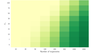
(a) Mean $\Pi_{b}$-SPIBB with $\eta=0.9$

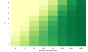
(b) Mean $\Pi_{\leq b}$-SPIBB with $\eta=0.9$

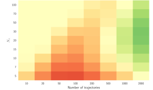
(c) 1%-CVaR $\Pi_{b}$-SPIBB with $\eta=0.9$

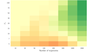
(d) 1%-CVaR $\Pi_{\leq b}$-SPIBB with $\eta=0.9$

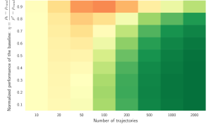
(e) 1%-CVaR $\Pi_{b}$-SPIBB ($N_{\wedge}=10$)

(f) 1%-CVaR $\Pi_{\leq b}$-SPIBB ($N_{\wedge}=10$)

Figure 6: Random MDPs (no additional goal): SPIBB hyper-parameter search results: (a-d) Mean and 1%-CVaR performance heatmaps as a function of $N_{\wedge}$ (e-f) 1%-CVaR performance heatmaps as a function of $\eta$ with the best hyper-parameter ($N_{\wedge}=10$).

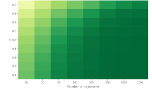
(a) Mean: Basic RL.

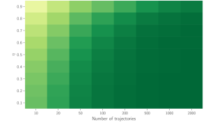
(b) Mean: RaMDP.

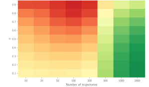
(c) Mean: Robust MDP.

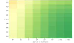
(d) Mean: HCPI doubly robust.

(e) Mean: $\Pi_{b}$-SPIBB.

(f) Mean: $\Pi_{\leq b}$-SPIBB.

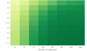
(g) Mean: Exact-Soft-SPIBB 1-step ($\epsilon=2$).

(h) Mean: Exact-Soft-SPIBB ($\epsilon=2$).

(i) Mean: Approx-Soft-SPIBB 1-step ($\epsilon=2$).

(j) Mean: Approx-Soft-SPIBB ($\epsilon=2$).

Figure 7: Random MDPs: mean performance heatmaps.

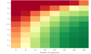
(a) 0.1%-CVaR: Basic RL.

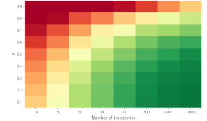
(b) 0.1%-CVaR: RaMDP.

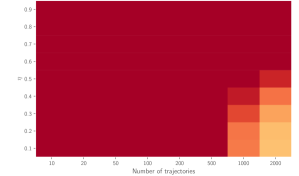
(c) 0.1%-CVaR: Robust MDP.

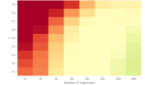
(d) 0.1%-CVaR: HCPI doubly robust.

(e) 0.1%-CVaR: $\Pi_{b}$-SPIBB.

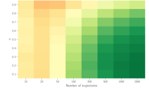
(f) 0.1%-CVaR: $\Pi_{\leq b}$-SPIBB.

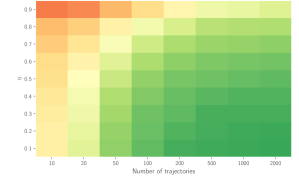
(g) 0.1%-CVaR: Exact-Soft-SPIBB 1-s ($\epsilon=2$).

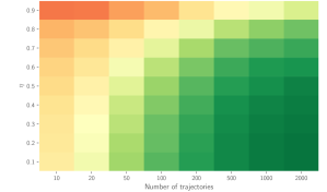
(h) 0.1%-CVaR: Exact-Soft-SPIBB ($\epsilon=2$).

(i) 0.1%-CVaR: Approx-Soft-SPIBB 1-s ($\epsilon=2$).

(j) 0.1%-CVaR: Approx-Soft-SPIBB ($\epsilon=2$).

Figure 8: Random MDPs: 0.1%-CVaR performance heatmaps.

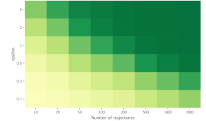
(a) Mean: Exact-Soft-SPIBB 1-step ($\eta=0.1$).

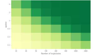
(b) Mean: Approx-Soft-SPIBB 1-step ($\eta=0.1$).

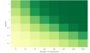
(c) Mean: Exact-Soft-SPIBB ($\eta=0.1$).

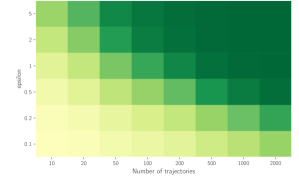
(d) Mean: Approx-Soft-SPIBB ($\eta=0.1$).

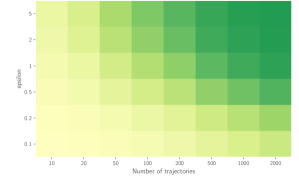
(e) Mean: Exact-Soft-SPIBB 1-step ($\eta=0.9$).

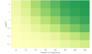
(f) Mean: Approx-Soft-SPIBB 1-step ($\eta=0.9$).

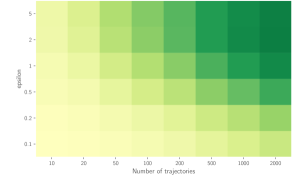
(g) Mean: Exact-Soft-SPIBB ($\eta=0.9$).

(h) Mean: Approx-Soft-SPIBB ($\eta=0.9$).

Figure 9: Random MDPs: hyper-parameter mean performance heatmaps for Soft-SPIBB methods under a weak ($\eta=0.1$) and a strong ($\eta=0.9$) baseline.

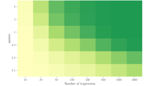
(a) 1%-CVaR: Exact-Soft-SPIBB 1-s ($\eta=0.1$).

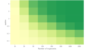
(b) 1%-CVaR: Approx-Soft-SPIBB 1-s ($\eta=0.1$).

(c) 1%-CVaR: Exact-Soft-SPIBB ($\eta=0.1$).

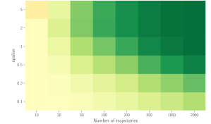
(d) 1%-CVaR: Approx-Soft-SPIBB ($\eta=0.1$).

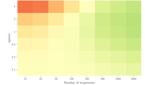
(e) 1%-CVaR: Exact-Soft-SPIBB 1-s ($\eta=0.9$).

(f) 1%-CVaR: Approx-Soft-SPIBB 1-s ($\eta=0.9$).

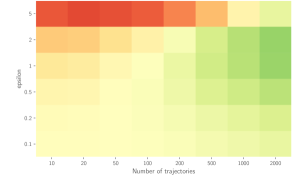
(g) 1%-CVaR: Exact-Soft-SPIBB ($\eta=0.9$).

(h) 1%-CVaR: Approx-Soft-SPIBB ($\eta=0.9$).

Figure 10: Random MDPs: hyper-parameter 1%-CVaR performance heatmaps for Soft-SPIBB methods under a weak ($\eta=0.1$) and a strong ($\eta=0.9$) baseline.

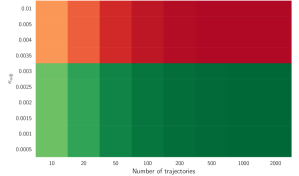
(a) Mean: RaMDP ($\eta=0.1$).

(b) 1%-CVaR: RaMDP ($\eta=0.1$).

(c) Mean: RaMDP ($\eta=0.4$).

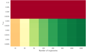
(d) 1%-CVaR: RaMDP ($\eta=0.4$).

(e) Mean: RaMDP ($\eta=0.6$).

(f) 1%-CVaR: RaMDP ($\eta=0.6$).

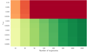
(g) Mean: RaMDP ($\eta=0.9$).

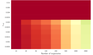
(h) 1%-CVaR: RaMDP ($\eta=0.9$).

Figure 11: Random MDPs: hyper-parameter mean and 1%-CVaR performance heatmaps for RaMDP methods under a weak ($\eta=0.1$), a medium weak ($\eta=0.4$), a medium strong ($\eta=0.6$), and a strong ($\eta=0.9$) baseline.

Appendix 0.C Helicopter experiment details

0.C.1 Details about the helicopter environment

See (Laroche et al.,, 2019, Appendix D.1).

0.C.2 Helicopter experimental process

See Pseudo-code 4.

Input: List of algorithms

Input: List of hyper-parameter values

Input: List of dataset sizes

repeat $20$ times

       for each dataset size do

            

            Generate a dataset.

            Compute the pseudo-counts.

            repeat $15$ times

                  

                  for each algorithm do

                         for each hyper-parameter value do

                              

                              Train a policy.

                              Evaluate the trained policy.

                              Record the performance of the trained policy.

Pseudo-code 4 Helicopter experimental process

0.C.3 Details about the DQN implementations

The batch version of DQN simply consists in replacing the experience replay buffer by the dataset we are training on. Effectively, we are not sampling from the environment anymore but from the transitions collected a priori following the baseline. RaMDP follows the same principle with a target modified according to the reward hacking:

$$y^{(i)}_{j} =r_{j}-\cfrac{\kappa}{\sqrt{\tilde{N}_{\mathcal{D}}(x_{j},a_{j})}}+\gamma\max_{a^{\prime}\in\mathcal{A}}Q^{(i)}(x_{j}^{\prime},a^{\prime}),$$ (86)

where $\tilde{N}_{\mathcal{D}}(x_{j},a_{j})$ is the pseudo-count. For the sake of simplicity and to be able to repeat several runs of each experiment efficiently, instead of applying pseudo-count methods from the literature (Bellemare et al.,, 2016; Fox et al.,, 2018; Burda et al.,, 2019), we consider here a pseudo-count heuristic based on the Euclidean state-distance, and a task where it makes sense to do so. The pseudo-count of a state-action $(x,a)$ is defined as the sum of its similarity with the state-action pairs $(x_{i},a_{i})$ found in the dataset. The similarity between $(x,a)$ and $(x_{i},a_{i})$ is equal to 0 if $a_{i}\neq a$, and to $\max(0,1-5d(x,x_{i}))$ otherwise, where $d(\cdot,\cdot)$ is the Euclidean distance between two states:

$$\tilde{N}_{\mathcal{D}}(x,a) =\sum_{\langle x_{j},a_{j}=a,r_{j},x^{\prime}_{j}\rangle\in\mathcal{D}}\max(0,1-5d(x,x_{j})),$$ (87)

The same pseudo-counts were used for all algorithms using it. In particular, they allowed to compute the error function at each state-action pair as (the cardinal of continuous state spaces cannot be used as in the tabular case):

$$e_{P}(x,a)=\frac{1}{\sqrt{\tilde{N}_{\mathcal{D}}(x,a)}}.$$ (88)

The same general methodology applies for Soft-SPIBB, according to the definitions from Section 3.2.4. Although, SPIBB is a special case of Soft-SPIBB, its implementation has been performed independently in order to be more computationally efficient. For SPIBB, the targets we are using for our $Q$-values updates verify the following modified Bellman equation:

$$y^{(i)}_{j} =r_{j}+\gamma\max_{\pi\in\Pi_{b}}\sum_{a^{\prime}\in\mathcal{A}}\pi(a^{\prime}|x_{j}^{\prime})Q^{(i)}(x_{j}^{\prime},a^{\prime})$$ (89)

$$=r_{j}+\gamma\sum_{(x_{j}^{\prime},a^{\prime})\in\mathfrak{B}}\pi_{b}(a^{\prime}|x_{j}^{\prime})Q^{(i)}(x_{j}^{\prime},a^{\prime})$$

$$\quad\quad+\gamma\left(\sum_{(x_{j}^{\prime},a^{\prime})\notin\mathfrak{B}}\pi_{b}(a^{\prime}|x_{j}^{\prime})\right)\max_{(x_{j}^{\prime},a^{\prime})\notin\mathfrak{B}}Q^{(i)}(x_{j}^{\prime},a^{\prime})$$ (90)

We notice in particular that when $\mathfrak{B}=\emptyset$ the targets fall back to the traditional Bellman ones. We used the now classic target network trick (Mnih et al.,, 2015), combined with Double-DQN (van Hasselt et al.,, 2015).

The network used for the baseline and for the algorithms in the benchmark is a fully connected network with 3 hidden layers of $32$, $128$ and $32$ neurons, initialized using he_uniform (He et al.,, 2015). The network has $9$ outputs corresponding to the $Q$-values of the $9$ actions in the game. We train the $Q$-networks with RMSProp (Tieleman and Hinton,, 2012) with a momentum of $0.95$ and $\epsilon=10^{-7}$ on mini-batches of size $32$. The learning rate is initialized at $0.01$ and is annealed every $20$k transitions or every pass on the dataset, whichever is larger. The networks are trained for $2$k passes on the dataset, and are fully converged by that time. The models are trained with Pytorch (Paszke et al.,, 2017). The policy is tested for $1$k steps at the end of training, with the initial states of each trajectory sampled as described in Section 0.C.1.

0.C.4 Additional experimental results

See Table 2 and Figure 12.

Table 2: Helicopter: numerical (mean and 10%-CVaR) results with optimal hyper-parameters

$|\mathcal{D}|$	Baseline		DQN		RaMDP-DQN		$\Pi_{b}$-SPIBB		Soft-SPIBB
	Mean	CVaR	Mean	CVaR	Mean	CVaR	Mean	CVaR	Mean	CVaR
1,000	2.30	1.59	-0.91	-1.00	N/A	N/A	2.74	1.91	2.72	1.88
3,000	2.30	1.59	-0.72	-1.00	0.85	-0.70	3.19	2.37	3.23	2.38
6,000	2.30	1.59	0.07	-1.00	N/A	N/A	3.30	2.41	3.39	2.54
10,000	2.30	1.59	0.22	-1.00	3.21	1.65	3.39	2.46	3.61	2.69

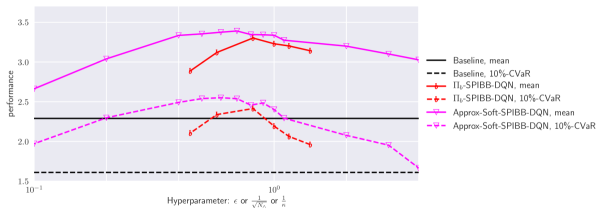
(a) Helicopter benchmark with $|\mathcal{D}|=6,000$

(b) Helicopter benchmark with $|\mathcal{D}|=1,000$

Figure 12: Helicopter: mean and 10%-CVaR as a function of the hyper-parameter

Appendix 0.D Reproducible, reusable, and robust Reinforcement Learning

This paper’s objective is to improve the robustness and the reliability of Reinforcement Learning algorithms. Inspired from Joelle Pineau’s talk at NeurIPS 2018 about reproducible, reusable, and robust Reinforcement Learning, we intend to also make our work reusable and reproducible.

0.D.1 Pineau’s checklist (slide 33)

For all algorithms presented, check if you include:

• A clear description of the algorithm.

  • See Section 3.

• An analysis of the complexity (time, space, sample size) of the algorithm.

  • We provide formal analysis for the complexity in Section 3.2.3, and a rapid empirical assessment in Figure 1 for the finite MDP analysis. For Soft-SPIBB-DQN, we empirically observed a $50\%$ increase in runtime compared to SPIBB-DQN.

• A link to downloadable source code, including all dependencies.

  • The code is being made available. The code will be made public on acceptation. See Section 0.D.2.

For any theoretical claim, check if you include:

• A statement of the result.

  • See Theorems 3.1, 3.2, and 3.4.

• A clear explanation of any assumptions.

  • The main assumption for Theorem 3.2 is formalized as Assumption 1. See Section 3 for discussion.

• A complete proof of the claim.

  • See Section 0.A.

For all figures and tables that present empirical results, check if you include:

• A complete description of the data collection process, including sample size.

  • See Sections 4, 0.B.1.1, and 0.C.1.

• A link to downloadable version of the dataset or simulation environment.

  • See Section 0.D.2.

• An explanation of how sample were allocated for training / validation / testing.

  • The complete dataset is used for training. There is no need for validation set. Testing is performed in the true environment.

• An explanation of any data that was excluded.

  • Does not apply to our simulated environments.

• The range of hyper-parameters considered, method to select the best hyper-parameter configuration, and specification of all hyper-parameters used to generate results.

  • See Sections 0.B.2 and 0.C.3.

• The exact number of evaluation runs.

  • 100,000+ for finite MDPs experiments and 300 for SPIBB-DQN experiments.

• A description of how experiments were run.

  • See Sections 4, 0.B, and 0.C.

• A clear definition of the specific measure or statistics used to report results.

  • Mean and X% conditional value at risk (CVaR), described in Sections 4 and 0.B.1.5.

• Clearly defined error bars.

  • Given the high number of runs we considered, the error bar are too thin to be displayed. Any difference visible with the naked eye is significant. We use CVaR everywhere instead to account for the uncertainty.

• A description of results including central tendency (e.g. mean) and variation (e.g. stddev).

  • All our work is motivated and analyzed with respect to this matter.

• The computing infrastructure used.

  • For the finite-MDPs experiment, we used clusters of CPUs. The full results were obtained by running the benchmarks with 100 CPUs running independently in parallel during 24h. For the helicopter experiment, we used a GPU cluster. However, only one GPU is necessary for a single run. Using a cluster allowed to launch several runs in parallel and considerably sped up the experiment. On a single GPU (a GTX 1080 Ti), a dataset of $|\mathcal{D}|=10$k transitions is generated in $~{}5$ seconds. The dataset generation scales linearly in $|\mathcal{D}|$. Computing the counts for that dataset takes approximately $20$ minutes, it scales quadratically with the size of the dataset. As far as training is concerned, $2000$ passes on a dataset of $10$k transitions takes around $25$ minutes, it scales linearly in $N$. Finally, evaluation of the trained policy on $10$k trajectories takes $15$ minutes. It scales linearly in $|\mathcal{D}|$ as it requires the computation of the pseudo-count for each state encountered during the evaluation and this pseudo-count computation is linear in $|\mathcal{D}|$. Overall, a single run for a dataset of $10$k transitions takes around one hour.

0.D.2 Code attached to the submission

The attached code can be used to reproduce the experiments presented in the submitted paper. It is split into two projects: one for finite MDPs, and one for Soft-SPIBB-DQN.

• https://github.com/RomainLaroche/SPIBB

• https://github.com/rems75/SPIBB-DQN

0.D.2.1 Finite MDPs

Prerequisites

The finite MDP project is implemented in Python 3.5 and only requires *numpy* and *scipy*.

Content

We include the following:

• Libraries of the following algorithms:

  • Basic RL,

  • Soft-SPIBB:

    • Exact-Soft-SPIBB (1-step or not),

    • Approx-Soft-SPIBB (1-step or not),

  • SPIBB:

    • $\Pi_{b}$-SPIBB,

    • $\Pi_{\leq b}$-SPIBB,

  • HCPI:

    • doubly-robust,

    • importance sampling,

    • weighted importance sampling,

    • weighted per decision IS,

    • per decision IS,

  • Robust MDP,

  • and Reward-adjusted MDP.

• Environments:

  • Random MDPs environment.

• Random MDPs experiment of Section 4.1. Run:

  python soft_randomMDPs_main.py #name_of_experiment# #random_seed#

Not included

We DO NOT include the following:

• The hyper-parameter search (appendix, Section 0.B.2): it should be easy to re-implement.

• The figure generator: it has too many specificities to be made understandable for a user at the moment. Also, it is not hard to re-implement with one’s own visualization tools.

License

This project is BSD-licensed.

0.D.2.2 Soft-SPIBB-DQN

Prerequisites

Soft-SPIBB-DQN is implemented in Python 3 and requires the following libraries: PyTorch, pickle, glob, yaml, argparse, numpy, yaml, pathlib, csv, scipy and click.

Content

The SoftSPIBB-DQN project contains the helicopter environment, the baseline used for our experiments and the code required to generate datasets and train vanilla DQN, RaMDP-DQN, SPIBB-DQN and Soft-SPIBB-DQN.

Not included

We DO NOT include the following:

• The multi-CPU/multi-GPU implementation: its structure is too much dependent on the cluster tools. It would be useless for somebody from another lab and might divulge author affiliations.

License

This project is BSD-licensed.

References

- Bellemare et al., (2016) Bellemare, M., Srinivasan, S., Ostrovski, G., Schaul, T., Saxton, D., and Munos, R. (2016). Unifying count-based exploration and intrinsic motivation. In Proceedings of the 29th Advances in Neural Information Processing Systems (NIPS).
- Borgwardt, (1987) Borgwardt, K. H. (1987). The Simplex Method: A Probabilistic Analysis. Springer-Verlag Berlin Heidelberg.
- Burda et al., (2019) Burda, Y., Edwards, H., Storkey, A., and Klimov, O. (2019). Exploration by random network distillation. In Proceedings of the 7th International Conference on Learning Representations (ICLR).
- Dantzig, (1963) Dantzig, G. (1963). Linear programming and extensions. Rand Corporation Research Study. Princeton Univ. Press, Princeton, NJ.
- Dantzig and Thapa, (2003) Dantzig, G. B. and Thapa, M. N. (2003). Linear Programming 2: Theory and Extensions. Springer-Verlag New York.
- Ernst et al., (2005) Ernst, D., Geurts, P., and Wehenkel, L. (2005). Tree-based batch mode reinforcement learning. Journal of Machine Learning Research, 6(Apr):503–556.
- Fox et al., (2018) Fox, L., Choshen, L., and Loewenstein, Y. (2018). Dora the explorer: Directed outreaching reinforcement action-selection. In Proceedings of the 6th International Conference on Learning Representations (ICLR).
- Geist et al., (2019) Geist, M., Scherrer, B., and Pietquin, O. (2019). A theory of regularized markov decision processes. In Proceedings of the 36th International Conference on Machine Learning (ICML).
- Gondzio, (2012) Gondzio, J. (2012). Interior point methods 25 years later. European Journal of Operational Research.
- Guez et al., (2008) Guez, A., Vincent, R. D., Avoli, M., and Pineau, J. (2008). Adaptive treatment of epilepsy via batch-mode reinforcement learning. In Proceedings of the 23rd AAAI Conference on Artificial Intelligence, pages 1671–1678.
- He et al., (2015) He, K., Zhang, X., Ren, S., and Sun, J. (2015). Delving deep into rectifiers: Surpassing human-level performance on imagenet classification. arXiv preprint arXiv:1502.01852.
- Iyengar, (2005) Iyengar, G. N. (2005). Robust dynamic programming. Mathematics of Operations Research.
- Kakade and Langford, (2002) Kakade, S. and Langford, J. (2002). Approximately optimal approximate reinforcement learning. In Proceedings of the 19th International Conference on Machine Learning (ICML), volume 2, pages 267–274.
- Klee and Minty, (1972) Klee, V. and Minty, G. J. (1972). How good is the simplex algorithm? In Shisha, O., editor, Inequalities, volume III, pages 159–175. Academic Press, New York.
- Lange et al., (2012) Lange, S., Gabel, T., and Riedmiller, M. (2012). Batch Reinforcement Learning, pages 45–73. Springer Berlin Heidelberg, Berlin, Heidelberg.
- Laroche et al., (2019) Laroche, R., Trichelair, P., and Tachet des Combes, R. (2019). Safe policy improvement with baseline bootstrapping. In Proceedings of the 36th International Conference on Machine Learning (ICML).
- Mnih et al., (2015) Mnih, V., Kavukcuoglu, K., Silver, D., Rusu, A. A., Veness, J., Bellemare, M. G., Graves, A., Riedmiller, M., Fidjeland, A. K., Ostrovski, G., et al. (2015). Human-level control through deep reinforcement learning. Nature, 518(7540):529.
- Nilim and El Ghaoui, (2005) Nilim, A. and El Ghaoui, L. (2005). Robust control of markov decision processes with uncertain transition matrices. Operations Research.
- Paszke et al., (2017) Paszke, A., Gross, S., Chintala, S., Chanan, G., Yang, E., DeVito, Z., Lin, Z., Desmaison, A., Antiga, L., and Lerer, A. (2017). Automatic differentiation in pytorch. In NIPS-W.
- Petrik et al., (2016) Petrik, M., Ghavamzadeh, M., and Chow, Y. (2016). Safe policy improvement by minimizing robust baseline regret. In Proceedings of the 29th Advances in Neural Information Processing Systems (NIPS).
- Riedmiller, (2005) Riedmiller, M. (2005). Neural fitted q iteration–first experiences with a data efficient neural reinforcement learning method. In Proceedings of the 16th European Conference on Machine Learning (ECML), pages 317–328. Springer.
- Schulman et al., (2015) Schulman, J., Levine, S., Abbeel, P., Jordan, M., and Moritz, P. (2015). Trust region policy optimization. In Proceedings of the 32nd International Conference on Machine Learning (ICML).
- Schulman et al., (2017) Schulman, J., Wolski, F., Dhariwal, P., Radford, A., and Klimov, O. (2017). Proximal policy optimization algorithms. arXiv preprint arXiv:1707.06347.
- Simão and Spaan, (2019) Simão, T. D. and Spaan, M. T. J. (2019). Safe policy improvement with baseline bootstrapping in factored environments. In Proceedings of the 32nd AAAI Conference on Artificial Intelligence.
- Singh et al., (1999) Singh, S. P., Kearns, M. J., Litman, D. J., and Walker, M. A. (1999). Reinforcement learning for spoken dialogue systems. In Proceedings of the 13st Advances in Neural Information Processing Systems (NIPS), pages 956–962.
- Sutton and Barto, (1998) Sutton, R. S. and Barto, A. G. (1998). Reinforcement Learning: An Introduction. The MIT Press.
- Thomas, (2015) Thomas, P. S. (2015). Safe reinforcement learning. PhD thesis, Stanford university.
- Tieleman and Hinton, (2012) Tieleman, T. and Hinton, G. (2012). Lecture 6.5-rmsprop: Divide the gradient by a running average of its recent magnitude. COURSERA: Neural networks for machine learning, 4(2):26–31.
- van Hasselt et al., (2015) van Hasselt, H., Guez, A., and Silver, D. (2015). Deep reinforcement learning with double q-learning. CoRR, abs/1509.06461.
- Weissman et al., (2003) Weissman, T., Ordentlich, E., Seroussi, G., Verdu, S., and Weinberger, M. J. (2003). Inequalities for the l1 deviation of the empirical distribution. Hewlett-Packard Labs, Tech. Rep.