Even maps, the Colin de Verdière number and representations of graphs

Abstract

Van der Holst and Pendavingh introduced a graph parameter $\sigma$, which coincides with the more famous Colin de Verdière graph parameter $\mu$ for small values. However, the definition of $\sigma$ is much more geometric/topological directly reflecting embeddability properties of the graph. They proved $\mu(G)\leq\sigma(G)+2$ and conjectured $\mu(G)\leq\sigma(G)$ for any graph $G$. We confirm this conjecture. As far as we know, this is the first topological upper bound on $\mu(G)$ which is, in general, tight.

Equality between $\mu$ and $\sigma$ does not hold in general as van der Holst and Pendavingh showed that there is a graph $G$ with $\mu(G)\leq 18$ and $\sigma(G)\geq 20$. We show that the gap appears on much smaller values, namely, we exhibit a graph $H$ for which $\mu(H)\leq 7$ and $\sigma(H)\geq 8$. We also prove that, in general, the gap can be large: The incidence graphs $H_{q}$ of finite projective planes of order $q$ satisfy $\mu(H_{q})\in O(q^{3/2})$ and $\sigma(H_{q})\geq q^{2}$.

1 Introduction

In 1990 [Col90] (English translation [Col91]) introduced a graph parameter $\mu(G)$. It arises from the study of the multiplicity of the second smallest eigenvalue of certain matrices associated to a graph $G$ (discrete Schrödinger operators); however, it turns out that this parameter is closely related to geometric and topological properties of $G$. In particular, this parameter is minor monotone, and moreover, it satisfies:

1. $\mu(G)=0$ if and only if $G$ embeds in $\mathbb{R}^{0}$;

2. $\mu(G)\leq 1$ if and only if $G$ embeds in $\mathbb{R}^{1}$;

3. $\mu(G)\leq 2$ if and only if $G$ is outer planar;

4. $\mu(G)\leq 3$ if and only if $G$ is planar; and

5. $\mu(G)\leq 4$ if and only if $G$ admits a linkless embedding into $\mathbb{R}^{3}$.

The characterization up to the value 3 as well as the minor monotonicity of $\mu$ was shown by [Col90, Col91]. The characterization of graphs with $\mu(G)\leq 4$ was established by [LS98]. Beyond this, any description is known only for the classes of graphs with $\mu(G)\geq\left|V(G)\right|-k$ for $k=1,2,3$ and partial results are known also for $k=4,5$; see [KLV97]. It used to be an open problem whether the graphs with $\mu(G)\leq 5$ coincide with knotless embeddable graphs [DW13, Sec. 14.5], [Tho99, Sec. 7]. However, a graph $H$ constructed by [Foi03] satisfies $\mu(H)\leq 5$ whereas it is not knotless embeddable. We are very thankful to Rose McCarty for sharing this example with us [McC19].

Due to the aforementioned properties, the study of $\mu$ gained a lot of popularity (e.g., [BC95, vdHol95, vdHLS95a, KLV97, LS98, vdHLS99, LS99, Lov01, Izm10, Gol13, SS17, McC18, Tai19]). A precise definition of the parameter $\mu$ is given at the end of Subsection 2.1.

Later, in 2009, [vdHP09] introduced another minor monotone parameter $\sigma(G)$, whose definition is much closer to the topological properties of $G$. Roughly speaking, $\sigma(G)$ is defined as a minimal integer $k$ such that every CW-complex $\mathcal{C}$ whose $1$-skeleton is $G$ admits a so-called even mapping into $\mathbb{R}^{k}$. This is a mapping $f$ such that whenever $\vartheta$ and $\tau$ are disjoint cells of $\mathcal{C}$, then $f(\vartheta)\cap f(\tau)=\emptyset$ if $\dim\vartheta+\dim\tau<k$, and $f(\vartheta)$ and $f(\tau)$ cross in an even number of points if $\dim\vartheta+\dim\tau=k$. For a precise definition, we refer to [vdHP09].

It turns out that $\sigma(G)\leq k$ if and only if $\mu(G)\leq k$ for $k\in\{0,1,2,3,4\}$. In addition, [vdHP09, Conj. 43 ] conjectured that this is true also for $k=5$. However, in general, $\sigma$ and $\mu$ differ. They provide an example of a graph with $\mu(G)\leq 18$, but $\sigma(G)\geq 20$ based on a previous work of [Pen98]. On the other hand, [vdHP09, Cor. 41 ] proved that $\mu(G)\leq\sigma(G)+2$, while they conjectured that $\mu(G)\leq\sigma(G)$. We confirm this conjecture.

Theorem 1.

For any graph $G$, $\mu(G)\leq\sigma(G)$.

Our tools that we use for the proof of Theorem 1 also allow us to show that the gap between $\mu$ and $\sigma$ appears at much smaller values.

Theorem 2.

There is a graph $G$ such that $\mu(G)\leq 7$ and $\sigma(G)\geq 8$.

We remark here that adding a new vertex to a graph $G$ and connecting it to all vertices of $G$ increases both $\mu(G)$ and $\sigma(G)$ by exactly one (unless $G$ is the complement of $K_{2}$); see [vdHLS99, Thm. 2.7] and [vdHP09, Thm. 28]. Consequently, Theorem 2 immediately implies that for every $k\in\mathbb{N},k\geq 7$ there is a graph $G_{k}$ with $\mu(G_{k})\leq k$ and $\sigma(G_{k})\geq k+1$.

The key step in the proof of Theorem 2 is to provide a lower bound on $\sigma$; otherwise we follow [Pen98]. We remark that the example of $G$ with $\mu(G)\leq 18$ but $\sigma(G)\geq 20$ coming from [vdHP09, Pen98] is highly regular Tutte’s 12-cage. The important property is that the second largest eigenvalue of the adjacency matrix of Tutte’s 12-cage has very high multiplicity. We use instead the incidence graphs of finite projective planes, which enjoy the same property. Namely, if $H_{q}$ is the incidence graph of a finite projective plane of order $q$, we will show that $\mu(H_{3})\leq 9$, whereas $\sigma(H_{3})\geq 11$; see Proposition 27. Then, by further modification of this graph, we obtain the graph from Theorem 2.

As a complementary result, based on properties of finite projective planes, we also show that the gap between $\mu$ and $\sigma$ is asymptotically large.

Theorem 3.

Let $q\in\mathbb{N}$ be such that a finite projective plane of order $q$ exists. Then $\mu(H_{q})\in O\left(q^{3/2}\right)$, while $\sigma(H_{q})\geq\lambda(H_{q})\geq q^{2}$, where $\lambda$ is the graph parameter of [vdHLS95], which we overview in Section 4.

Further motivation and computational aspects.

If we are interested only in the properties of the Colin de Veridère parameter $\mu$, Theorem 1 can be reformulated as: If $\sigma(G)\leq k$, then $\mu(G)\leq k$. In other words, if $G$ has a nice geometric description in $\mathbb{R}^{k}$, then $\mu(G)\leq k$. This is tight in general because $\mu(K_{n})=\sigma(K_{n})=n-1$, where $K_{n}$ is the complete graph on $n$ vertices [vdHLS99, vdHP09]. As far as we can say this is the first tight upper bound on $\mu(G)$ taking into account embeddability properties of $G$ for general value of the parameter.

On the other hand, we would also like to argue that the parameter $\sigma$ deserves comparable attention as $\mu$.

First of all, it provides a much more direct geometric generalization of graph planarity than the parameter $\mu$; more in a spirit of the Hanani–Tutte type characterization of graph planarity (see, e.g.,  [Sch13]).

Next, it seems that it might be computationally much more tractable to determine the graphs with $\sigma\leq k$ when compared to graphs with $\mu\leq k$. From now on, let $\mathsf{G}_{\mu\leq k}$ and $\mathsf{G}_{\sigma\leq k}$ denote the class of graphs with $\mu\leq k$ and $\sigma\leq k$ respectively. Of course, once we fix an integer $k$, there is a polynomial time algorithm for recognition of graphs in $\mathsf{G}_{\mu\leq k}$ and $\mathsf{G}_{\sigma\leq k}$ via the Robertson–Seymour theory [RS95, RS04] as there is a finite list of forbidden minors for these classes. The minors are well known if $k\leq 4$; however the catch of this approach is that it seems to be out of reach to find the minors as soon as $k\geq 5$.

Let us focus on the interesting case $k=5$. We are not aware of any explicit algorithm for determining the graphs in $\mathsf{G}_{\mu\leq 5}$ in the literature. The best algorithm we could come up with is a PSPACE algorithm based on the existential theory of the reals. (This algorithm recognizes the graphs in $\mathsf{G}_{\mu\leq k}$ for general $k\in\mathbb{N}$.) For completeness we describe it in Appendix A.

On the other hand, there is a completely different set of tools for recognition of graphs $G$ from $\mathsf{G}_{\sigma\leq 5}$. According to [vdHP09, Thm. 30] it is sufficient to verify whether the $2$-skeleton of a so-called closure of $G$ admits an even mapping into $\mathbb{R}^{4}$. We do not describe here a closure of $G$ in general; however, according to the definition in [vdHP09], it can be chosen in such a way that its $2$-skeleton coincides with the complex obtained by gluing a disk to each cycle of $G$; let us denote this complex by $\mathcal{C}^{2}(G)$. It is in general well known that it can be determined whether a $2$-complex admits an even mapping to $\mathbb{R}^{4}$ (even in polynomial time in the size of the complex). From the point of view of algebraic topology, this is equivalent to vanishing of the $\mathbb{Z}_{2}$-reduction of the so-called van Kampen obstruction. An explicit algorithm can be found in [MTW11] modulo small modifications caused by the facts that $\mathcal{C}^{2}(G)$ is not a simplicial complex and that we work with the $\mathbb{Z}_{2}$-reduction. The algorithm runs in time polynomial in size of $\mathcal{C}^{2}(G)$, which might be exponential in size of $G$. However, the naive implementation of the algorithm seems to perform many redundant checks. By removing some of these redundancies, we can get an explicit polynomial time certificate for $\sigma(G)>5$, that is, a certificate for co-NP membership. A proof of this is given in Appendix B. Optimistically, we may hope that this algorithm could be adapted to an explicit polynomial time algorithm.

Now, if the conjecture $\mathsf{G}_{\mu\leq 5}=\mathsf{G}_{\sigma\leq 5}$ of van der Holst and Pendavingh is true, then the algorithm above also determines graphs with $\mu\leq 5$. Theorem 1 gives one implication.

Similar ideas can perhaps be used for the recognition of graphs from $\mathsf{G}_{\sigma\leq k}$ with general $k$, though this requires working with the $\lfloor(k-1)/2\rfloor$-skeleton of the closure, which is more complicated. (Of course, the impact on $\mu$ is then more limited due to Theorems 2 and 3.)

Overview of our proofs.

Here we briefly overview the key steps in our main proofs. We start with Theorem 1. On high level, we follow [LS98], who showed that if $G$ is a linklessly embeddable graph, then $\mu(G)\leq 4$. First we sketch (in our words) their strategy and then we point out the important differences.

For contradiction, Lovász and Schrijver assume that there is linklessly embeddable $G$ with $\mu(G)\geq 5$. According to the definition of $\mu$ (given in the next section), there is a certain matrix $M\in\mathbb{R}^{V\times V}$ of corank $5$ associated to $G=(V,E)$ which witnesses $\mu(G)\geq 5$. Given a vector $x\in\mathbb{R}^{V}$, we denote by $\operatorname{supp}(x)$ the set $\left\{v\in V\colon x_{v}\neq 0\right\}$. Correspondingly, we define $\operatorname{supp}_{+}(x):=\left\{v\in V\colon x_{v}>0\right\}$ and $\operatorname{supp}_{-}(x):=\left\{v\in V\colon x_{v}<0\right\}$. Then $\ker(M)$, the kernel of $M$, can be decomposed into equivalence classes of vectors for which $\operatorname{supp}_{+}$ and $\operatorname{supp}_{-}$ coincide. Each equivalence class is a (relatively open) cone (see Definition 11). Then, by choosing a suitably dense set of unit vectors in each of the cones and taking the convex hull, Lovász and Schrijver obtain a $5$-dimensional polytope $\mathbf{P}$ such that every relatively open face of $\partial\mathbf{P}$ is in one of the cones.

Given a linkless embedding of $G$ (more precisely, a flat embedding), it is possible now to define an embedding $f$ of the $1$-skeleton $\mathbf{P}^{(1)}$ into $\mathbb{R}^{3}$ in such a way that for every vertex $\mathbf{u}$ of $\mathbf{P}$, which is also a vector of $\ker(M)$, $f(\mathbf{u})$ is mapped close to a vertex of $\operatorname{supp}_{+}(\mathbf{u})$ (this vertex is embedded in $\mathbb{R}^{3}$ by the given linkless/flat embedding of $G$).

Also, for every edge $\mathbf{e}=\mathbf{u}\mathbf{w}$ of $\mathbf{P}$, we have $\operatorname{supp}_{+}(\mathbf{e})\supseteq\operatorname{supp}_{+}(\mathbf{u}),\operatorname{supp}_{+}(\mathbf{w})$. If $G[\operatorname{supp}_{+}(\mathbf{e})]$, the subgraph induced by $\operatorname{supp}_{+}(\mathbf{e})$, is connected for every such $\mathbf{e}$, then Lovász and Schrijver pass $f(\mathbf{e})$ close to some path connecting $f(\mathbf{u})$ and $f(\mathbf{w})$ in $G[\operatorname{supp}_{+}(\mathbf{e})]$. An existence of such $f$ then reveals that the original embedding of $G$ was not linkless via a Borsuk–Ulam type theorem by [LS98], which is the required contradiction.

It, however, still remains to resolve the case when some edges $\mathbf{e}$ do not satisfy that $G[\operatorname{supp}_{+}(\mathbf{e})]$ is connected. Such edges are called broken edges and it is the main technical part of the proof to take care of them. Via structural properties of $G$, including the usage of one of the forbidden minors for linkless embeddability (see [RST95] for the list of minimal such graphs), Lovász and Schrijver show how to route the broken edges without introducing new linkings, which again yields the required contradiction.

Our main technical contribution is that we design a strategy how to route broken edges without any requirements on the structure of $G$. Namely, we show that if we make several very careful choices in the very beginning when placing the vertices of $\mathbf{P}$ as well as if we carefully route the nonbroken edges of $\mathbf{P}$, then we are able to make enough space for broken edges as well. The important property is that when $\mathbf{F}$ and $\mathbf{F}^{\prime}$ are (so-called) antipodal faces, then the edges of $\mathbf{F}$ and the edges of $\mathbf{F}^{\prime}$ are routed close to disjoint subgraphs. (The precise statement is given by Proposition 23, and we actually map $\mathbf{P}^{(1)}$ into the graph $G$.)

Now, we could aim to conclude in a similar way as Lovász and Schrijver via a suitable Borsuk–Ulam type theorem, which would require to extend the map to higher skeletons and to perturb it a bit. However, we instead use a lemma of [vdHP09] tailored to such a setting, which they used in the proof of the inequality $\mu(G)\leq\sigma(G)+2$ (see the proof of Proposition 22).

Last but not least, instead of working directly with matrices from the definition of $\mu$, we abstract their properties required in the proof of Theorem 1 into a notion of semivalid representation; see Definition 5. (The main difference is that we replace the so-called Strong Arnold hypothesis by more combinatorial properties.) This abstraction turns out to be very useful in the proof of Theorem 2 because then it is possible to provide lower bounds on $\sigma$ also with aid of matrices not satisfying the Strong Arnold hypothesis, which is essential if we want to separate $\mu$ and $\sigma$.

Recall that by $H_{q}$ we denote the incidence graph of a finite projective plane of order $q$. We add a short description of how our bound on $\sigma(G)$ is used in the proof of Theorem 2; here we only sketch how to show a slightly weaker result $\sigma(H_{3})\geq 11$, discussed below the statement of Theorem 2. We first note that semivalid representations are defined as certain linear subspaces of $\mathbb{R}^{V}$ and we will introduce a parameter $\eta(G)$ which is the maximal dimension of a semivalid representation. We will also show $\mu(G)\leq\eta(G)\leq\sigma(G)$, where $\mu(G)\leq\eta(G)$ follows easily from the known results on $\mu$ whereas showing the inequality $\eta(G)\leq\sigma(G)$ is the core of the proof of Theorem 1.

Now let us consider a matrix $M_{3}$ which is a suitable shift of the adjacency matrix of $H_{3}$. This matrix satisfies $\operatorname{corank}(M_{3})=\dim\ker(M_{3})=12$ and $\ker M_{3}$ is ‘almost’ a semivalid representation of $G$. Namely, by a trick that we learnt from [Pen98] we can find a codimension 1 subspace $L$ of $\ker(M)$ which is a semivalid representation. This shows $\eta(H_{3})\geq 11$ and the key inequality $\sigma(G)\geq\eta(G)$ gives the required bound $\sigma(H_{3})\geq 11$.

The proof of Theorem 3 follows the same high-level strategy as the proof of Theorem 2, except we do not work there with a semivalid representation, but rather with a so-called valid representation, which is a concept used to define the parameter $\lambda$ (see Subsection 2.2). We use a simple general position argument to show that if $G$ has a low maximum degree, then a large subspace of $\ker(M_{q})$ has to be a valid representation of $G$ where $M_{q}$ is, in analogy to the previous case, a suitable shift of the adjacency matrix of $H_{q}$.

Organization.

In Section 2 we overview (or introduce) various representations of graphs and establish some of their properties. Then we prove Theorem 1 in Section 3 and Theorems 2 and 3 in Section 4.

2 Representations of graphs

2.1 The Colin de Verdière graph parameter

If not stated otherwise, we work with a graph $G=(V,E)$. We use the usual graph-theoretic notation $N(v)$ for all vertices adjacent to $v\in V$ and $N(S)$ for all vertices in $V\setminus S$ adjacent to a vertex in $S\subseteq V$. Moreover, we use $G[S]$ to denote the subgraph of $G$ induced by $S$. For a set $S\subset V$ we denote by $x_{S}$ the restriction of the vector $x$ to the subset $S$, that is, $x_{S}:=(x_{v})_{v\in S}$.

Let $\mathcal{M}(G)$ be the set of symmetric matrices $M$ in $\mathbb{R}^{V\times V}$ satisfying

1. $M$ has exactly one negative eigenvalue of multiplicity one,

2. for any $u\neq v\in V$, $uv\in E$ implies $M_{uv}<0$ and $uv\notin E$ implies $M_{u,v}=0$.

The matrices satisfying only the second of the properties above are sometimes called discrete Schrödinger operators in the literature.

Note that there is no condition on the diagonal entries of $M$. Despite this, a part of the Perron–Frobenius theory is still applicable to $M\in\mathcal{M}(G)$, assuming that $G$ is connected (if not, the same reasoning can be applied component-wise). This is because the matrix $-M+cI_{V}$, where $I_{V}$ denotes the identity matrix of size $V\times V$, has nonnegative entries for $c>0$ large enough. Since this transformation preserves all eigenspaces, the Perron–Frobenius theorem implies that the smallest eigenvalue of $M$ has multiplicity one and the corresponding eigenvector is strictly positive (or strictly negative). For instance, as $M$ has an orthogonal eigenbasis, this implies that every nonzero vector $x\in\ker(M)$ must have both $\operatorname{supp}_{+}(x)$ and $\operatorname{supp}_{-}(x)$ nonempty.

A matrix $M\in\mathcal{M}(G)$ satisfies the so-called Strong Arnold hypothesis (SAH), if

$$MX=0\qquad\Longrightarrow\qquad X=0$$

for every symmetric $X\in\mathbb{R}^{V\times V}$ such that $X_{u,v}=0$ whenever $u=v$ or $uv\in E$. The Colin de Verdière graph parameter $\mu(G)$ is defined as the maximum of $\operatorname{corank}(M)$ over matrices $M\in\mathcal{M}(G)$ satisfying SAH.

2.2 Semivalid representations of graphs

We collect some of the easy, but important properties of matrices in $\mathcal{M}(G)$ in the following lemma. The proofs can be found, for instance, in a survey by [vdHLS99, Sec. 2.5 ].

Lemma 4.

Let $G=(V,E)$ be a connected graph and $M\in\mathcal{M}(G)$. Let $x\in\ker(M)$ be nonzero, then

1. $N(\operatorname{supp}(x))=N(\operatorname{supp}_{-}(x))\cap N(\operatorname{supp}_{+}(x))$,

2. if $G[\operatorname{supp}_{+}(x)]$ is disconnected, then there is no edge between $\operatorname{supp}_{+}(x)$ and $\operatorname{supp}_{-}(x)$, and moreover, for every connected component $C$ of $G[\operatorname{supp}(x)]$ we have $N(C)=N(\operatorname{supp}(x))$,

3. if $\operatorname{supp}(x)$ is inclusion-minimal among nonzero vectors in $\ker(M)$, then both graphs $G[\operatorname{supp}_{+}(x)]$ and $G[\operatorname{supp}_{-}(x)]$ are nonempty and connected.

Motivated by the parameter $\mu$, [vdHLS95] introduced the invariant $\lambda(G)$ defined as follows. We say that a linear subspace $X\subseteq\mathbb{R}^{V}$ is a valid representation of the graph $G$, if for every nonzero $x\in X$ the graph $G[\operatorname{supp}_{+}(x)]$ is nonempty and connected. Then $\lambda(G)$ is defined as the maximum of $\dim(X)$ over all valid representations $X$ of $G$.

Among other properties, [vdHLS95] proved that $\lambda$ is minor monotone and characterized the classes of graphs with $\lambda(G)\leq 1,2,3$. From this characterization it follows that the parameters $\lambda$ and $\mu$ differ already for those small values. In general, $\lambda$ can be both greater or smaller than $\mu$ (see [vdHLS95, Pen98]).

Somewhat analogously to the notion of a valid representation, we introduce the following definition:

Definition 5 (Semivalid representation).

Given a connected graph $G=(V,E)$ we call a linear subspace $L\subseteq\mathbb{R}^{V}$ a semivalid representation of $G$ if, for every nonzero $x\in L$,

1. both $\operatorname{supp}_{+}(x)$ and $\operatorname{supp}_{-}(x)$ are nonempty,

2. the graph $G[\operatorname{supp}_{+}(x)]$ is either connected, or $G[\operatorname{supp}_{+}(x)]$ has two connected components and $G[\operatorname{supp}_{-}(x)]$ is connected,

3. if $x$ has inclusion-minimal support in $L$, both $G[\operatorname{supp}_{+}(x)]$ and $G[\operatorname{supp}_{-}(x)]$ are nonempty and connected,

4. if $G[\operatorname{supp}_{+}(x)]$ is disconnected, then there is no edge between $\operatorname{supp}_{+}(x)$ and $\operatorname{supp}_{-}(x)$, and moreover, for every connected component $C$ of $G[\operatorname{supp}(x)]$ we have $N(C)=N(\operatorname{supp}(x))$.

We will use semivalid representations of $G$ as a substitute for $\ker(M)$ in case we want to work with $M$ not necessarily satisfying SAH. This is enabled by the following lemma taken from [Pen98], which together with Lemma 4 implies that the kernel of $M\in\mathcal{M}(G)$ satisfying SAH defines a semivalid representation of $G$:

Lemma 6 ([Pen98, Lem. 3]).

Let $G$ be a connected graph and $M\in\mathcal{M}(G)$. Let $x\in\ker(M)$ and set

$$D:=\left\{y\in\ker(M)\colon\operatorname{supp}(y)\subseteq\operatorname{supp}(x)\right\}.$$

If $G[\operatorname{supp}(x)]$ is disconnected, it has exactly $\dim(D)+1$ connected components. If, in addition, $M$ satisfies SAH, then $\dim(D)\leq 2$.

Similarly to the graph parameter $\lambda$ introduced by [vdHLS95], we define an analogous parameter $\eta(G)$:

Definition 7.

Let $G$ be a graph. If $G$ is connected, we define

$$\eta(G):=\max\left\{\dim(L)\colon L\text{ is a semivalid representation of }G\right\}.$$

For convenience, we also extend the definition to disconnected graphs $G$. If $G$ has at least one edge, then we define

$$\eta(G):=\max_{C}\eta\left(G[C]\right),$$

where the maximum is taken over connected components $C$ of $G$. If $G$ is disconnected and does not have any edge, then we set $\eta(G):=1$.

Lemmas 4 and 6 show that $\mu(G)\leq\eta(G)$ for every connected graph $G$. The definition of $\eta$ for disconnected graphs is chosen in a way that agrees precisely with the behavior of $\mu$: In [vdHLS99, Thm. 2.5] it is shown that $\mu(G)$ is equal to the maximum of $\mu$ over the connected components of $G$ if $G$ has at least one edge. Moreover, it is easy to see that $\mu$ of the empty graph on $n\geq 2$ vertices is $1$ (or see, e.g., [vdHLS99, Sec. 1.2]).

Comparing the definitions of valid and semivalid representations, it is clear that every valid representation is also a semivalid representation. Since for disconnected graphs $\lambda$ exhibits exactly the same type of behavior as $\mu$ and $\eta$ with respect to the connected components, which is easy to see directly from the definition of $\lambda$, we get that $\eta(G)$ is always an upper bound on $\lambda(G)$ for any graph $G$. Summarizing, we get the following:

Observation 8.

For every graph $G$ it holds that $\max\left\{\mu(G),\lambda(G)\right\}\leq\eta(G)$.∎

2.3 Topological preliminaries

Polyhedra.

A set $\tau^{\prime}\subset\mathbb{R}^{k}$ is a closed (convex) polyhedron if it is an intersection of finitely many closed half-spaces. A closed face of a polyhedron $\tau^{\prime}$ is a subset $\eta^{\prime}\subseteq\tau^{\prime}$such that there exists a hyperplane $h$ satisfying that $\eta^{\prime}=h\cap\tau^{\prime}$ and $\tau^{\prime}$ belongs to one of the closed half-spaces determined by $h$. A relatively open polyhedron is the relative interior $\tau$ of a closed polyhedron $\tau^{\prime}$ (the relative interior is taken with respect to the affine hull of $\tau^{\prime}$).

Important convention.

In the sequel, when we say polyhedron, we mean relatively open polyhedron. This is nonstandard, but it will be very convenient for our considerations. Given a polyhedron $\tau$, by $\overline{\tau}$ we denote the closure of $\tau$, that is, the corresponding closed polyhedron. We also say that a (relatively open) polyhedron $\eta$ is a face of $\tau$ if $\overline{\eta}$ is a closed face of $\overline{\tau}$.

Polyhedral complexes.

A polyhedral complex is a collection $\mathcal{C}$ of polyhedra satisfying:

1. If $\tau\in\mathcal{C}$ and $\eta$ is a face of $\tau$, then $\eta\in\mathcal{C}$.

2. If $\theta,\tau\in\mathcal{C}$, then $\overline{\theta}\cap\overline{\tau}$ is a closed face of $\overline{\theta}$ as well as a closed face of $\overline{\tau}$.

The body of a polyhedral complex $\mathcal{C}$ is defined as $|\mathcal{C}|:=\bigcup\mathcal{C}$. Due to our convention that we consider relatively open polyhedra, $|\mathcal{C}|$ is a disjoint union of polyhedra contained in $\mathcal{C}$.

Given a polyhedron $\tau$, by $\partial\tau$ we denote the boundary of $\tau$. With a slight abuse of notation, depending on the context, this may be understood both as a polyhedral complex formed by the proper faces of $\tau$ as well as the topological boundary of $\tau$, that is, the body of the former one.

The $k$-skeleton of a polyhedral complex $\mathcal{C}$ is the subcomplex $\mathcal{C}^{(k)}$ consisting of all faces of $\mathcal{C}$ of dimension at most $k$.

In our considerations, we will need two special classes of polyhedra: simplicial complexes and fans.

Simplicial complexes.

A polyhedral complex is a simplicial complex if each polyhedron in the complex is a simplex. (Consistently with our convention above, by a simplex we mean a relatively open simplex.)

Fans.

A cone is a polyhedron $\alpha\subseteq\mathbb{R}^{k}$ such that $rx\in\alpha$ whenever $x\in\alpha$ and $r\in(0,\infty)$. A polyhedral complex $\mathcal{F}$ is a fan if each polyhedron in $\mathcal{F}$ is a cone, and moreover, if $\mathcal{F}$ contains a nonempty polyhedron, then $\mathcal{F}$ contains the origin as a polyhedron. A fan is complete if $|\mathcal{F}|=\mathbb{R}^{k}$.

Subdivisions.

Let $\mathcal{C}$ be a polyhedral complex. A polyhedral complex $\mathcal{D}$ is a subdivision of $\mathcal{C}$ if $|\mathcal{C}|=|\mathcal{D}|$ and for every $\eta\in\mathcal{D}$, there is $\tau$ in $\mathcal{C}$ containing $\eta$.

Fans and polytopes.

By a polytope we mean a bounded polyhedron. Let $\mathbf{P}\subseteq\mathbb{R}^{k}$ be a polytope such that the origin is in the interior of $\mathbf{P}$. Then $\mathbf{P}$ defines a complete fan $\mathcal{F}(\mathbf{P})$ formed by the cones over the proper faces of $\mathbf{P}$ (plus the empty set). Again, we consider the faces of $\mathbf{P}$ relatively open. With a slight abuse of terminology, we say that $\mathbf{P}$ subdivides a fan $\mathcal{F}^{\prime}$ if $\mathcal{F}(\mathbf{P})$ subdivides $\mathcal{F}^{\prime}$; see Figure 1.

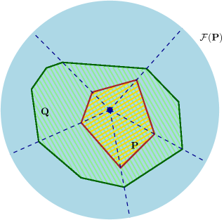
Figure 1: A polytope $\mathbf{P}$, the fan $\mathcal{F}(\mathbf{P})$ and a polytope $\mathbf{Q}$ subdividing $\mathcal{F}(\mathbf{P})$.

Barycentric subdivisions.

Now let $\mathcal{K}$ be a simplicial complex. For every nonempty simplex $\tau\in K$ let $b_{\tau}$ be the barycenter of $\tau$. For two faces $\eta$ and $\tau$ of $\mathcal{K}$, let $\eta\prec\tau$ denote that $\eta$ is a proper face of $\tau$. The barycentric subdivision of $\mathcal{K}$, denoted $\operatorname{sd}\mathcal{K}$, is a simplicial complex obtained so that for every chain $\Gamma=\theta_{1}\prec\theta_{2}\prec\cdots\prec\theta_{m}$ of nonempty faces of $\mathcal{K}$ we add a simplex, denoted $\Delta(\Gamma)$, with vertices $b_{\theta_{1}},\dots,b_{\theta_{m}}$ into $\operatorname{sd}\mathcal{K}$. It is well known that $\operatorname{sd}\mathcal{K}$ subdivides $\mathcal{K}$. In particular, $\Delta(\Gamma)\subset\theta_{m}$.

Observation 9.

Let $\mathcal{K}$ be a simplicial complex and $\Delta$ be a simplex of the barycentric subdivision $\operatorname{sd}\mathcal{K}$. Let $\Delta_{1}$ and $\Delta_{2}$ be two faces of $\Delta$ and $\eta_{1}\supseteq\Delta_{1}$ and $\eta_{2}\supseteq\Delta_{2}$ be two faces of $\mathcal{K}$. Then either $\eta_{1}$ is a face of $\eta_{2}$ or $\eta_{2}$ is a face of $\eta_{1}$.

Proof.

The face $\Delta$ corresponds to a chain $\Gamma=\theta_{1}\prec\cdots\prec\theta_{m}$ of faces of $\mathcal{K}$. Then $\Delta_{1}$ corresponds to a subchain $\Gamma_{1}$ of $\Gamma$ with maximal face $\theta_{i}$ (for some $i$). Then $\theta_{i}$ is the (unique) face of $\mathcal{K}$ containing $\Delta_{1}=\Delta(\Gamma_{1})$. Therefore $\eta_{1}=\theta_{i}$. Similarly, $\eta_{2}=\theta_{j}$ for some $j$, from which the conclusion follows. ∎

Before we state the next lemma, we introduce two more well-known notions. Let $\mathcal{K}$ be a simplicial complex and $|\mathcal{L}|$ be the body of some subcomplex $\mathcal{L}$ of $\mathcal{K}$. We define the simplicial neighborhood of $|\mathcal{L}|$ in $\mathcal{K}$ as

$$\mathcal{N}(|\mathcal{L}|,\mathcal{K}):=\{\eta\in\mathcal{K}\colon\eta\subset\overline{\tau}\hbox{ for some }\tau\hbox{ with }\overline{\tau}\cap|\mathcal{L}|\neq\emptyset\}.$$

If $\mathcal{L}$ consists of a single vertex $a$, then the simplicial neighborhood is known as (closed) star of $a$ in $\mathcal{K}$, denoted by $\operatorname{st}(a;\mathcal{K})$.

Lemma 10.

Let $\mathcal{K}$ be a simplicial complex and let $\mathcal{L}_{1},\mathcal{L}_{2}$ be two subcomplexes of $\mathcal{K}$ with $|\mathcal{L}_{1}|\cap|\mathcal{L}_{2}|=\emptyset$. Let $a$ be a vertex of the second barycentric subdivision $\operatorname{sd}^{2}\mathcal{K}$. Then the closed star $\operatorname{st}(a;\operatorname{sd}^{2}\mathcal{K})$ cannot intersect both $|\mathcal{L}_{1}|$ and $|\mathcal{L}_{2}|$.

Proof.

The closed star $\operatorname{st}(a;\operatorname{sd}^{2}\mathcal{K})$ intersects $|\mathcal{L}_{i}|$ only if $a$ belongs to $\mathcal{N}(|\mathcal{L}_{i}|,\operatorname{sd}^{2}\mathcal{K})=\mathcal{N}(|\operatorname{sd}^{2}\mathcal{L}_{i}|,\operatorname{sd}^{2}\mathcal{K})$. The lemma follows from the fact that $\mathcal{N}(|\mathcal{L}_{1}|,\operatorname{sd}^{2}\mathcal{K})$ and $\mathcal{N}(|\mathcal{L}_{2}|,\operatorname{sd}^{2}\mathcal{K})$ are disjoint. (This is a simple exercise on properties of simplicial/derived/regular neighborhoods using the tools from [RS82]. An explicit reference for this claim we are aware of is Corollary 4.5 in [TT13]—embedding in a manifold assumed in [TT13] plays no role in the proof.) ∎

Stellar subdivisions of polytopes.

Let $\mathbf{P}\subseteq\mathbb{R}^{k}$ be a polytope such that the origin belongs to the interior of $\mathbf{P}$ and let $\mathbf{F}$ be a face of $\mathbf{P}$. Let $\mathbf{a}$ be a point beyond all facets (i.e. maximal faces) $\mathbf{F}^{\prime}$ of $\mathbf{P}$ such that $\overline{\mathbf{F}}\subseteq\overline{\mathbf{F}^{\prime}}$ (that is, $\mathbf{a}$ and the origin are on different sides of the hyperplane defining $\mathbf{F}^{\prime}$) whereas $\mathbf{a}$ is beneath all other facets ($\mathbf{a}$ and the origin are on the same side of the defining hyperplane). Then the polytope $\mathbf{P}^{\prime}$ obtained as the convex hull of the set of vertices of $\mathbf{P}$ and $\mathbf{a}$ is called a geometric stellar subdivision of $\mathbf{P}$ [ES74]. For any $\mathbf{F}$, we can pick $\mathbf{a}$ as above lying inside the cone of $\mathcal{F}(\mathbf{P})$ containing $\mathbf{F}$. Let $p\colon\partial\mathbf{P}^{\prime}\to\partial\mathbf{P}$ be the projection towards the origin. Then the complex $p(\partial\mathbf{P}^{\prime}):=\{p(\mathbf{F}^{\prime})\colon\mathbf{F}^{\prime}\hbox{ is a proper face of }\mathbf{P}^{\prime}\}$ is a subdivision of the boundary of $\mathbf{P}$. Consequently, $\mathcal{F}(\mathbf{P}^{\prime})$ subdivides $\mathcal{F}(\mathbf{P})$.

If we perform stellar subdivisions gradually on all proper faces of a polytope $\mathbf{P}$ ordered by nonincreasing dimension, we obtain a simplicial polytope. In fact, we get a polytope isomorphic to a barycentric subdivision of $\mathbf{P}$; however, we will use this stronger conclusion only when $\mathbf{P}$ is already simplicial. That is, in this case we obtain a polytope $\mathbf{P}^{\prime}$ such that the projection $p\colon\partial\mathbf{P}^{\prime}\to\partial\mathbf{P}$ is a simplicial isomorphism between $\partial\mathbf{P}^{\prime}$ and $\operatorname{sd}\partial\mathbf{P}$ provided in each step, when performing individual stellar subdivisions over face $\mathbf{F}$, the newly added point $\mathbf{a}$ is on the ray from the origin containing the barycenter of $\mathbf{F}$. For more details on stellar and barycentric subdivisions of polytopes, we refer to [ES74].

2.4 Fan of a semivalid representation

Given a semivalid representation $L$ of $G$ we now aim to build a fan $\mathcal{P}=\mathcal{P}(L)$ (complete in $L$) formed by convex polyhedral cones in a way that corresponds to splitting $L$ by hyperplanes passing through the origin and perpendicular to the standard basis vectors of $\mathbb{R}^{V}$.

Definition 11 (Fan $\mathcal{P}(L)$).

Let $L$ be a semivalid representation of $G$ and let us define an equivalence relation $\sim$ on $\mathbb{R}^{V}$ by

$$x\sim y\qquad\Longleftrightarrow\qquad\operatorname{supp}_{+}(x)=\operatorname{supp}_{+}(y)\text{ and }\operatorname{supp}_{-}(x)=\operatorname{supp}_{-}(y).$$

Each equivalence class $[x]_{\sim}$ is a convex cone in $\mathbb{R}^{V}$ (relatively open), and we define $\mathcal{E}$ to be the fan formed by these cones.

Then we define $\mathcal{P}=\mathcal{P}(L)$ as the fan obtained by intersecting $\mathcal{E}$ with $L$. In other words, the cones of $\mathcal{P}$ are the equivalence classes of $\sim$ restricted to $L$.

If the semivalid representation $L$ is irrelevant or understood from the context, we omit it from the notation and write just $\mathcal{P}$. We refer to a $k$-dimensional cone as to a $k$-cone.

We extend the notation of support to cones in $\mathcal{P}$, i.e., if $\alpha\in\mathcal{P}$, then $\operatorname{supp}_{\pm}(\alpha):=\operatorname{supp}_{\pm}(x)$ for some $x\in\alpha$. Also, if $A\subseteq\alpha$ for some $\alpha$ in $\mathcal{P}$, then $\operatorname{supp}_{\pm}(A):=\operatorname{supp}_{\pm}(\alpha)$.

We continue with several observations on properties of $\mathcal{P}$.

Observation 12.

Let $\alpha,\beta$ be two cones of $\mathcal{P}$. Then $\alpha\subseteq\partial\beta$ if and only if

$$\operatorname{supp}_{+}(\alpha)\subseteq\operatorname{supp}_{+}(\beta)\quad\text{ and }\quad\operatorname{supp}_{-}(\alpha)\subseteq\operatorname{supp}_{-}(\beta)$$

and at least one of the inclusions is strict.

Proof.

The equivalence follows immediately from the facts that $\partial\beta\subseteq\overline{\beta}$ and $\overline{\beta}$ contains all $y\in L$ with $\operatorname{supp}_{+}(y)\subseteq\operatorname{supp}_{+}(\beta)$ and $\operatorname{supp}_{-}(y)\subseteq\operatorname{supp}_{-}(\beta)$. At least one of the inclusions is strict if and only if $\alpha\neq\beta$. ∎

Corollary 13.

Whenever $\alpha,\beta$ are two cones of $\mathcal{P}$ such that $\alpha\subseteq\partial\beta$, then $\operatorname{supp}_{+}(\beta)\subseteq V\setminus\operatorname{supp}_{-}(\alpha)$.

Proof.

Indeed, $\operatorname{supp}_{+}(\beta)\subseteq V\setminus\operatorname{supp}_{-}(\beta)\subseteq V\setminus\operatorname{supp}_{-}(\alpha)$. ∎

Corollary 14.

A cone $\alpha$ of $\mathcal{P}=\mathcal{P}(L)$ is a 1-cone if and only if the vectors of $\alpha$ have inclusion-minimal support among nonzero vectors in $L$.

Proof.

If $\alpha$ is a 1-cone, then every vector in $\alpha$ has to have inclusion-minimal support among nonzero vectors in $L$ due to Observation 12. On the other hand, if $\alpha$ contains vectors $x$ with inclusion-minimal supports, then $\dim(\alpha)=1$, otherwise there were two linearly independent vectors $x,y\in\alpha$ and $x-\varepsilon y\in L$ would have strictly smaller support than $x,y$ for an appropriate choice of $\varepsilon>0$. ∎

Definition 15.

If $G[\operatorname{supp}_{+}(x)]$ is disconnected for a nonzero $x\in\mathbb{R}^{V}$, we call $x$ a broken vector. The cones of $\mathcal{P}$ consisting of broken vectors are called broken cones.

In the remainder of the present subsection, we always assume that $G=(V,E)$ is a connected graph, $L\subseteq\mathbb{R}^{V}$ is a semivalid representation of $G$ and $\mathcal{P}:=\mathcal{P}(L)$ is the fan corresponding to $L$.

Lemma 16.

Let $\beta$ be a broken cone of $\mathcal{P}$ and $\alpha$ be a cone of $\mathcal{P}$ with $\alpha\subseteq\partial\beta$. Then

1. $\operatorname{supp}_{-}(\alpha)=\operatorname{supp}_{-}(\beta)$,

2. $G[\operatorname{supp}_{+}(\alpha)]$ is equal to a single connected component of $G[\operatorname{supp}_{+}(\beta)]$, and

3. $\alpha$ is a 1-cone.

Proof.

For $W\subseteq V=V(G)$ by a (connected) component of $W$ we always mean the vertex set of a connected component of $G[W]$. Observation 12 says that $\operatorname{supp}_{+}(\alpha)\subseteq\operatorname{supp}_{+}(\beta)$, $\operatorname{supp}_{-}(\alpha)\subseteq\operatorname{supp}_{-}(\beta)$, and at least on of the inclusions is strict. Throughout the proof, $a$ is a vector in $\alpha$ and $b$ in $\beta$.

First, we deduce that $\operatorname{supp}_{+}(\alpha)$ contains at least one of the two components of $\operatorname{supp}_{+}(\beta)$. For contradiction, we assume that $\operatorname{supp}_{+}(\beta)\setminus\operatorname{supp}_{+}(\alpha)$ is not contained in a single component of $\operatorname{supp}_{+}(\beta)$. Consider the vector $b-Ka$ for $K>0$ sufficiently large. Then

$$\operatorname{supp}_{+}(b-Ka)=\left(\operatorname{supp}_{+}(\beta)\setminus\operatorname{supp}_{+}(a)\right)\cup\operatorname{supp}_{-}(a).$$

Definition 5((iv)) applied to $b$ implies that $\operatorname{supp}_{-}(a)$ is in a different component of $\operatorname{supp}_{+}(b-Ka)$ than $\operatorname{supp}_{+}(\beta)\setminus\operatorname{supp}_{+}(a)$. Together with the assumption above this means that $\operatorname{supp}_{+}(b-Ka)$ has at least three components, which contradicts Definition 5((ii)). Let us denote by $C_{1}$ a component of $\operatorname{supp}_{+}(\beta)$ contained in $\operatorname{supp}_{+}(\alpha)$ and let $C_{2}$ be the other component.

By similar ideas we deduce ((i)). For contradiction, suppose that $\operatorname{supp}_{-}(\alpha)\subsetneq\operatorname{supp}_{-}(\beta)$. This time, we consider the vector $Ka-b$ for $K>0$ sufficiently large. The component $\operatorname{supp}_{-}(\beta)$ thus contributes both to $\operatorname{supp}_{+}(Ka-b)$ and $\operatorname{supp}_{-}(Ka-b)$. The component $C_{1}$ of $\operatorname{supp}_{+}(\beta)$ is inside $\operatorname{supp}_{+}(Ka-b)$. No matter whether the component $C_{2}$ of $\operatorname{supp}_{+}(\beta)$ contributes to $\operatorname{supp}_{+}(Ka-b)$ or $\operatorname{supp}_{-}(Ka-b)$ or both, in each case, we deduce a contradiction with Definition 5((ii))—either we have three components in the positive support or at least two components in the positive support and two components in the negative support. In particular, $\operatorname{supp}_{-}(\alpha)=\operatorname{supp}_{-}(\beta)$ implies that $\operatorname{supp}_{+}(\alpha)\subsetneq\operatorname{supp}_{+}(\beta)$.

Again by similar ideas we deduce ((ii)). Now we know that $C_{2}$ is not contained in $\operatorname{supp}_{+}(\alpha)$ because $\operatorname{supp}_{+}(\alpha)\subsetneq\operatorname{supp}_{+}(\beta)$. Then $C_{2}\cap\operatorname{supp}_{+}(\alpha)=\emptyset$, otherwise for $K>0$ sufficiently large $\operatorname{supp}_{+}(b-Ka)$ and $\operatorname{supp}_{-}(b-Ka)$ have two components each.

Finally, all this implies that $\alpha$ is a $1$-cone via Corollary 14 as ((i)) and ((ii)) (applied to $\alpha^{\prime}$) show that there is no $\alpha^{\prime}$ with its support strictly included in $\alpha$. ∎

The following observation is a generalization of part (8) from the proof of [LS98, Thm. 3 ], but the present proof is different to that of [LS98], since we work with a more general object than a kernel of a matrix in $\mathcal{M}(G)$.

Observation 17 (generalized [LS98]).

Let $\beta$ be a broken cone of $\mathcal{P}(L)$. Then

1. $\dim(\beta)=2$ and

2. $\partial\beta$ consists of two $1$-cones, which correspond to vectors $x\in L$ for which $\operatorname{supp}_{-}(x)=\operatorname{supp}_{-}(\beta)$ and $\operatorname{supp}_{+}(x)$ is identical with one of the connected components induced by $\operatorname{supp}_{+}(\beta)$.

Proof.

First we observe that if $\beta$ was only a 1-cone, then any $x\in\beta$ would have inclusion-minimal support in $L$ due to Corollary 14, which would be a contradiction to Definition 5((iii)).

Now let $\alpha$ be a cone from $\partial\beta$. Then Lemma 16 implies that $\alpha$ is a $1$-cone, $\operatorname{supp}_{-}(\alpha)=\operatorname{supp}_{-}(\beta)$ and $\operatorname{supp}_{+}(\alpha)$ is equal to exactly one of two connected components induced by $\operatorname{supp}_{+}(\beta)$. Therefore, we see that there are at most two different choices for $\alpha$, which are necessarily $1$-cones. Given that $\partial\beta\neq\emptyset$, because the closure of $\beta$ does not contain (nonzero) opposite points of $L$, and since $\dim(\beta)\geq 2$ we deduce that $\dim(\beta)=2$ by comparing the dimensions of the intersections of $\beta$ and $\partial\beta$ with the unit sphere in $L$ centered at the origin. Consequently, $\partial\beta$ consists of two $1$-cones. ∎

Notation.

For $x\in L$ we write $S(x):=N(\operatorname{supp}(x))$ and $R(x):=V\setminus\left(\operatorname{supp}(x)\cup S(x)\right)$. Let $\beta\in\mathcal{P}$. We write $S(\beta):=S(x)$ and $R(\beta):=R(x)$ for any $x\in\beta$. The notation is motivated by the fact that $S(x)$ is a ‘separator’ if $x$ is a broken vector and $R(x)$ is the set of vertices of $G$ ‘remote’ from $\operatorname{supp}(x)$; see Figure 2.

Figure 2: A typical picture of a separation of $G$ by $S(x)$ when $x$ is a broken vector in a semivalid representation. Compare with Lemma 4((ii)) and Definition 5.

Observation 18.

Let $\beta\in\mathcal{P}$ be broken. Then for every $x\in L$ such that $x_{S(\beta)}=0$ we have $x_{R(\beta)}=0$.

Proof.

Let $y\in\beta$ and assume, for contradiction, that there is $x\in L$ such that $x_{S(\beta)}=0$ and $x_{R(\beta)}\neq 0$. Since there is no edge between $R(\beta)$ and $\operatorname{supp}(y)$ in $G$, the set $\operatorname{supp}_{+}(y+\varepsilon x)$ is still disconnected and $\operatorname{supp}(y+\varepsilon x)$ induces at least four connected components, for all $\varepsilon>0$ small enough. This is incompatible with Definition 5((ii)). ∎

A crucial observation for our subsequent considerations is the following:

Observation 19.

Let $\alpha$ be a 1-cone of $\mathcal{P}$. Then there is at most one broken cone $\beta\in\mathcal{P}$ such that $\alpha\subseteq\overline{\beta}$.

Proof.

Let $\beta,\gamma$ be two broken cones such that $\alpha\subseteq\overline{\beta}\cap\overline{\gamma}$. By Observation 17((ii)) we get that $\operatorname{supp}_{-}(\beta)=\operatorname{supp}_{-}(\alpha)=\operatorname{supp}_{-}(\gamma)$. Definition 5((iv)) then implies that $S(\gamma)=S(\beta)$. Applying Observation 18 finishes the argument. ∎

2.5 Polytopal representation

In analogy with the approach of [LS98], we utilize semivalid representations $L$ of a given connected graph $G$ to build convex polytopes of dimension $\dim(L)$. By a $k$-face (or a $k$-cell) we mean a face (or a cell) of dimension $k$. We refer to a $d$-dimensional polytope as to a $d$-polytope.

Definition 20 (Polytopal representation).

Let $L$ be a semivalid representation of $G$, and $\mathcal{P}=\mathcal{P}(L)$ be the complete fan corresponding to $L$. We say that a polytope $\mathbf{P}\subset L$ containing the origin in its interior (relative in $L$) is polytopal representation of $G$ if it satisfies the following conditions.

1. The vertex set of $\mathbf{P}$ is centrally symmetric.

2. $\mathbf{P}$ subdivides $\mathcal{P}$. This in particular means, that for every face $\mathbf{F}$ of $\mathbf{P}$, there is a unique cone of $\mathcal{P}$ which contains $\mathbf{F}$. We denote this cone by $\gamma(\mathbf{F})$.

3. $\mathbf{P}$ is simplicial, that is, all faces of $\mathbf{P}$ are simplices.

4. Let $\mathbf{E}$, $\mathbf{F}$ be faces of $\partial\mathbf{P}$ which are faces of a common face of $\partial\mathbf{P}$. Then either $\gamma(\mathbf{E})$ is a face of $\gamma(\mathbf{F})$ or $\gamma(\mathbf{F})$ is a face of $\gamma(\mathbf{E})$. (This includes the option $\gamma(\mathbf{E})=\gamma(\mathbf{F})$.)

5. Let us define a broken edge as an edge of $\mathbf{P}$ lying in a broken cone of $\mathcal{P}$. Then we require: For every $\mathbf{a}\in\mathbf{P}^{(0)}$ all broken edges of $\mathbf{P}$ in $\operatorname{st}(\mathbf{a};\mathbf{P})$ belong to the same broken cone.

We, of course, need to know that a polytopal representation exists. [LS98] build a polytope $\mathbf{P}$ satisfying ((i))–((iii)) and a weaker version of ((iv)) as a convex hull of a sufficiently dense set of unit vectors taken from every cone, without going into details about how to choose this set. As we add extra properties, we want to be more careful and check that all of them can be satisfied.

Proposition 21.

Given a semivalid representation $L$, a corresponding polytopal representation $\mathbf{P}$ always exists.

Proof.

We start with considering the crosspolytope $\mathbf{C}\subseteq\mathbb{R}^{V}$ whose vertices are the standard basis vectors $e_{v}\in\mathbb{R}^{V}$ and their negatives $-e_{v}$ for $v\in V(G)$. Then the fan of the crosspolytope $\mathcal{F}(\mathbf{C})$ is exactly the fan $\mathcal{E}$ defined in Definition 11. Next we consider the auxiliary polytope $\mathbf{Q}:=\mathbf{C}\cap L$ and we get $\mathcal{P}=\mathcal{F}(\mathbf{Q})$. In particular, $\mathbf{Q}$ subdivides $\mathcal{P}$.

Subsequently, we apply a series of geometric stellar subdivisions on $\mathbf{Q}$ as described in Subsection 2.3. First we get a simplicial polytope $\mathbf{Q}^{\prime}$ which subdivides $\mathcal{P}$. Then we take $\mathbf{P}$ as the second barycentric subdivision of $\mathbf{Q}^{\prime}$, again by a series of stellar subdivisions. We perform all stellar subdivisions in a centrally symmetric fashion so that we obtain centrally symmetric $\mathbf{P}$.

It remains to verify the properties from Definition 20. The properties ((i)), ((ii)), and ((iii)) follow immediately from the construction.

We will show that ((iv)) follows from Observation 9. Let $\mathbf{Q}^{\prime\prime}$ be the polytope obtained from $\mathbf{Q}^{\prime}$ after the first barycentric subdivision and let $p^{\prime\prime}\colon\partial\mathbf{P}\to\partial\mathbf{Q}^{\prime\prime}$ be the projection towards the origin, as in Subsection 2.3. Then $p^{\prime\prime}(\partial\mathbf{P})$ is a barycentric subdivision of $\partial\mathbf{Q}^{\prime\prime}$. Now, let $\mathbf{E}^{\prime\prime}$ be the face of $\mathbf{Q}^{\prime\prime}$ containing $p^{\prime\prime}(\mathbf{E})$ and let $\mathbf{F}^{\prime\prime}$ be the face of $\mathbf{Q}^{\prime\prime}$ containing $p^{\prime\prime}(\mathbf{F})$; see Figure 3. Note that $\mathbf{E}^{\prime\prime}\subseteq\gamma(\mathbf{E})$. Indeed, $\mathbf{Q}^{\prime\prime}$ subdivides $\mathcal{P}$, therefore $\mathbf{E}^{\prime\prime}$ is contained in some cone of $\mathcal{P}$, and $\gamma(\mathbf{E})$ is the only option. Similarly, $\mathbf{F}^{\prime\prime}\subseteq\gamma(\mathbf{F})$. By Observation 9, $\mathbf{E}^{\prime\prime}$ is a face of $\mathbf{F}^{\prime\prime}$ or vice versa (the observation is applied with $\eta_{1}=\mathbf{E}^{\prime\prime}$, $\eta_{2}=\mathbf{F}^{\prime\prime}$, $\Delta_{1}=\mathbf{E}$, and $\Delta_{2}=\mathbf{F}$). Therefore $\gamma(\mathbf{E})$ is a face of $\gamma(\mathbf{F})$ or vice versa.

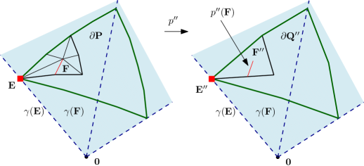
Figure 3: A picture ilustrating property ((iv)). In this picture, $L$ is $3$-dimensional. Left: The faces $\mathbf{E}$ and $\mathbf{F}$ are a vertex and an edge in a common (small) triangle of $\partial\mathbf{P}$. The larger (black) subdivided triangle containing both $\mathbf{E}$ and $\mathbf{F}$ is a result of applying a barycentric subdivision to (some triangle of) $\mathbf{Q}^{\prime\prime}$. The green outer ‘almost’ triangle depicts the intersection of $\partial\mathbf{P}$ and the cone $\gamma(\mathbf{F})$. Right: The picture shows $\mathbf{E}^{\prime\prime}$ and $\mathbf{F}^{\prime\prime}$ obtained as faces of $\mathbf{Q}^{\prime\prime}$ containing $p^{\prime\prime}(\mathbf{E})$ and $p^{\prime\prime}(\mathbf{F})$. In the specific case on the picture $p^{\prime\prime}(\mathbf{E})$ concides with $\mathbf{E}$ and $\mathbf{E}^{\prime\prime}$, thus only $p^{\prime\prime}(\mathbf{F})$ is depicted.

Finally, we derive ((v)) from Lemma 10. This time, we consider the projection $p^{\prime}\colon\mathbf{P}\to\mathbf{Q}^{\prime}$. Then $p^{\prime}(\partial\mathbf{P})$ is the second barycentric subdivision of $\partial\mathbf{Q}^{\prime}$. For contradiction, assume that the edges of $\operatorname{st}(\mathbf{a};\mathbf{P})$ belong to two broken cones $\beta_{1}$ and $\beta_{2}$. Equivalently, the edges of $\operatorname{st}(p^{\prime}(\mathbf{a});p^{\prime}(\partial\mathbf{P}))=\operatorname{st}(p^{\prime}(\mathbf{a});\operatorname{sd}^{2}(\partial\mathbf{Q}^{\prime}))$ belong to $\beta_{1}$ and $\beta_{2}$. Let $\mathcal{L}_{1}$ and $\mathcal{L}_{2}$ be subcomplexes of $\partial\mathbf{Q}^{\prime}$ triangulating $\overline{\beta_{1}}$ and $\overline{\beta_{2}}$, respectively. Observation 19 implies that $|\mathcal{L}_{1}|\cap|\mathcal{L}_{2}|=\emptyset$. Then, by Lemma 10, $\operatorname{st}(p^{\prime}(\mathbf{a});\operatorname{sd}^{2}(\partial\mathbf{Q}^{\prime}))$ cannot intersect both $|\mathcal{L}_{1}|$ and $|\mathcal{L}_{2}|$, a contradiction. ∎

3 On the relation $\mu(G)\leq\sigma(G)$

The aim of this section is to prove Theorem 1. In fact, we prove that $\eta(G)\leq\sigma(G)$ for every graph $G$. This immediately implies Theorem 1 thanks to Observation 8.

To make our exposition more readable, in the present section we refer to vertices and edges of a graph as to nodes and arcs, respectively, and reserve the terms vertices and edges for the 0- and 1-faces of polytopes.

Proposition 22.

Let $G$ be a connected graph and $L$ be a semivalid representation of $G$. Then $\dim(L)\leq\sigma(G)$.

The key step for the proof of Proposition 22 is to deduce Proposition 23 below. Given a polytope $\mathbf{Q}$, two faces $\mathbf{F}$ and $\mathbf{F}^{\prime}$ are antipodal if there exist two distinct parallel hyperplanes (relatively in the affine hull of $\mathbf{Q}$) $h$ and $h^{\prime}$ such that $\mathbf{F}\subset h$, $\mathbf{F}^{\prime}\subset h^{\prime}$ and $\mathbf{Q}$ is ‘between’ $h$ and $h^{\prime}$, that is, it belongs to one of the closed halfspaces bounded by $h$ as well as one of the closed halfspaces bounded by $h^{\prime}$. If $\mathbf{Q}$ is centrally symmetric, then $\mathbf{F}$ and $\mathbf{F}^{\prime}$ are antipodal if and only if $\mathbf{F}$ and $-\mathbf{F}^{\prime}$ belong to the closure of some proper face of $\mathbf{Q}$.

Given two polyhedral complexes $\mathcal{C}$ and $\mathcal{D}$, a map $f\colon|\mathcal{C}|\to|\mathcal{D}|$ is cellular if $f(\mathcal{C}^{(k)})\subseteq\mathcal{D}^{(k)}$ for every $k\geq 0$. If $\mathcal{C}$ and $\mathcal{D}$ are graphs, which is the only case we are interested in, then this condition means that every vertex of $\mathcal{C}$ is mapped to a vertex of $\mathcal{D}$.

Proposition 23.

Let $G$ be a connected graph and $\mathbf{P}$ a polytopal representation of $G$ (arising from the fan $\mathcal{P}=\mathcal{P}(L)$, where $L$ is a semivalid representation of $G$). Then, there is a cellular map $f\colon\mathbf{P}^{(1)}\to G$ such that for every pair of antipodal faces $\mathbf{F}$ and $\mathbf{F}^{\prime}$, the smallest subgraphs of $G$ containing $f(\mathbf{F}^{(1)})$ and $f(\mathbf{F}^{\prime(1)})$, respectively, have no common nodes.

Using the tools of van der Holst and Pendavingh [vdHP09], Proposition 23 implies Proposition 22 quite straightforwardly. As this proof is short, we present it before a proof of Proposition 23. Here, we essentially only repeat the proof of [vdHP09, Thm. 40].

Proof of Proposition 22..

The main tool for this proof is Lemma 37 from [vdHP09]. This lemma says that, under the additional assumption that $\mathbf{P}$ does not contain parallel faces (that is, faces with disjoint affine hulls such that $\mathbf{F}-\mathbf{F}$ and $\mathbf{F}^{\prime}-\mathbf{F}^{\prime}$ contain a common nonzero vector), the existence of $f$ from Proposition 23 implies $\sigma(G)\geq\dim\mathbf{P}$. (Note that $\dim\mathbf{P}=\dim L$.) Our $\mathbf{P}$ contains parallel faces. However, as van der Holst and Pendavingh point out, $\mathbf{P}$ can be perturbed by a projective transformation to a polytope without antipodal parallel faces preserving the combinatorial structure of the polytope. Similarly as van der Holst and Pendavingh do, we refer to the proof of [LS98, Thm. 1] for details. ∎

Notation.

Given $G$, $L$, $\mathcal{P}$ and $\mathbf{P}$ as in the statement of Proposition 23, we extend the notation $R(\gamma)$ and $S(\gamma)$ from cones to faces of $\mathbf{P}$. Let $\mathbf{F}$ be a face of $\mathbf{P}$, which lies in a unique cone $\gamma(\mathbf{F})\in\mathcal{P}$ by Definition 20. We define $S(\mathbf{F}):=S(\gamma(\mathbf{F}))$ and $R(\mathbf{F}):=R(\gamma(\mathbf{F}))$. Note also that $\operatorname{supp}(\mathbf{F})=\operatorname{supp}(\gamma(\mathbf{F}))$ and $\operatorname{supp}_{\pm}(\mathbf{F})=\operatorname{supp}_{\pm}(\gamma(\mathbf{F}))$ according to our convention above Observation 12.

Proof of Proposition 23..

During the construction, for each face $\mathbf{F}$ of $\mathbf{P}$ we will introduce a set $W(\mathbf{F})$, which will be a subset of nodes of $G$ such that $f(\mathbf{F}^{(1)})\subseteq G[W(\mathbf{F})]$. The key property of the construction will be that $W(\mathbf{F})$ and $W(\mathbf{F}^{\prime})$ are disjoint if $\mathbf{F}$ and $\mathbf{F}^{\prime}$ are antipodal faces of $\mathbf{P}$. We first define $f$ and $W$ on the vertices of $\mathbf{P}$ and then on the edges of $\mathbf{P}$. Finally, we extend the definition of $W$ to higher-dimensional faces and verify the required disjointness condition.

Throughout the proof, we repeatedly use the fact that every broken cone is $2$-dimensional according to Observation 17((i)). In particular, faces of $\mathbf{P}$ lying in a broken cone are either broken edges, or ‘inner’ vertices in a broken $2$-cone.

Before we start the construction, for every broken cone $\beta$ we fix a node $v(\beta)\in S(\beta)$. We also use the notation $v(\mathbf{b}):=v(\beta)$, where $\mathbf{b}$ is an arbitrary broken edge lying in $\beta$, that is, $\gamma(\mathbf{b})=\beta$.

Dimension $0$.

Given $\mathbf{u}\in\mathbf{P}^{(0)}$, Definition 20((v)) applied to $\mathbf{a}=-\mathbf{u}$ implies that either there is no broken edge antipodal to $\mathbf{u}$, or there is a unique $2$-cone $\beta=\beta(\mathbf{u})\in\mathcal{P}$ such that all broken edges antipodal to $\mathbf{u}$ lie in $\beta$. In the former case, we let $f(\mathbf{u})$ be an arbitrary node of $\operatorname{supp}_{+}(\mathbf{u})$. In the latter case, we want to avoid $R(\beta)$ and $v(\beta)$; thus, we need to check that we can do so.

Claim 23.1.

If $\beta=\beta(\mathbf{u})$ exists, then there is a node in $\operatorname{supp}_{+}(\mathbf{u})\setminus R(\beta)$ different from $v(\beta)$.

Proof.

We distinguish two cases according to whether $\gamma(-\mathbf{u})\subseteq\overline{\beta}$ or not.

If $\gamma(-\mathbf{u})\subseteq\overline{\beta}$, we get

$$\operatorname{supp}_{+}(\mathbf{u})=\operatorname{supp}_{-}(-\mathbf{u})\subseteq\operatorname{supp}_{-}(\beta)$$

whereas $v(\beta)$ does not belong to $\operatorname{supp}(\beta)$. Therefore the claim follows from the facts that $\operatorname{supp}_{+}(\mathbf{u})$ is nonempty by Definition 5((i)) and $R(\beta)\cap\operatorname{supp}(\beta)=\emptyset$.

Now we assume that $\gamma(-\mathbf{u})\not\subseteq\overline{\beta}$. Let $\mathbf{b}$ be an arbitrary broken edge antipodal to $\mathbf{u}$. We know that $\beta=\gamma(\mathbf{b})$. We also know that there is a proper face $\mathbf{F}$ of $\mathbf{P}$ such that $\mathbf{b}$ and $-\mathbf{u}$ belong to $\mathbf{F}$. Definition 20((iv)) implies that $\beta$ is a face of $\gamma(-\mathbf{u})$ or vice versa. Since $\gamma(-\mathbf{u})\not\subseteq\overline{\beta}$, we obtain that $\gamma(-\mathbf{u})$ is at least 3-dimensional cone satisfying $\beta\subseteq\overline{\gamma(-\mathbf{u})}$.

Now we get $\operatorname{supp}_{+}(\mathbf{u})=\operatorname{supp}_{-}(-\mathbf{u})\supseteq\operatorname{supp}_{-}(\beta)$. We also again use that $v(\beta)$ does not belong to $\operatorname{supp}(\beta)$. Therefore, the claim follows from the fact that $\operatorname{supp}_{-}(\beta)$ is nonempty and $R(\beta)\cap\operatorname{supp}(\beta)=\emptyset$. ∎

Therefore, if $\beta=\beta(\mathbf{u})$ exists, by Claim 23.1, we may set $f(\mathbf{u})$ to be an arbitrary node of $\operatorname{supp}_{+}(\mathbf{u})\setminus R(\beta)$ different from $v(\beta)$.

We also set, somewhat trivially, $W(\mathbf{u}):=\left\{f(\mathbf{u})\right\}$.

Dimension $1$.

Let $\mathbf{e}=\mathbf{u}\mathbf{w}$ be an edge of $\mathbf{P}$. We want to define $f$ on $\mathbf{e}$ as well as $W(\mathbf{e})$. We proceed so that for every edge $\mathbf{e}=\mathbf{u}\mathbf{w}$ of $\mathbf{P}$ we first suitably define $W(\mathbf{e})$ in such a way that $f(\mathbf{u})$ and $f(\mathbf{w})$ are nodes in the same connected component of $G[W(\mathbf{e})]$. Then we set $f(\mathbf{e})$ to be an arbitrary path connecting $f(\mathbf{u})$ and $f(\mathbf{w})$ inside $G[W(\mathbf{e})]$.

If $\mathbf{e}=\mathbf{b}$ is a broken edge, then we set $W(\mathbf{b}):=\operatorname{supp}_{+}(\mathbf{b})\cup\{v(\mathbf{b})\}$. Then $f(\mathbf{u})$ and $f(\mathbf{w})$ are nodes in $W(\mathbf{b})$ as $\operatorname{supp}_{+}(\mathbf{u}),\operatorname{supp}_{+}(\mathbf{w})\subseteq\operatorname{supp}_{+}(\mathbf{b})$. Also, $G[W(\mathbf{b})]$ is connected as $v(\mathbf{b})$ is adjacent to every component of $G[\operatorname{supp}(\mathbf{b})]$ by Definition 5((iv)).

Now, let us assume that $\mathbf{e}$ is not broken. For the connectedness of $G[W(\mathbf{e})]$ it would suffice to set $W(\mathbf{e})=\operatorname{supp}_{+}(\mathbf{e})$. We know that $G[\operatorname{supp}_{+}(\mathbf{e})]$ is connected as $\mathbf{e}$ is not broken, and also, $f(\mathbf{u})$ and $f(\mathbf{w})$ are nodes of $G[W(\mathbf{e})]$ by the same argument as above. However, in some cases we want $W(\mathbf{e})$ to be smaller; namely, if there is a broken edge $\mathbf{b}$ antipodal to $\mathbf{e}$, we want to avoid $v(\mathbf{b})$. Note that the cone $\beta:=\gamma(\mathbf{b})$ is independent of the choice of $\mathbf{b}$, if $\mathbf{b}$ exists, by Definition 20((v)) applied to an arbitrary vertex of $-\mathbf{e}$ in place of $\mathbf{a}$. Then $v(\mathbf{b})=v(\beta)$, $R(\mathbf{b})=R(\beta)$ and $S(\mathbf{b})=S(\beta)$ are independent of $\mathbf{b}$ as well. So, we set $W(\mathbf{e}):=\operatorname{supp}_{+}(\mathbf{e})$ if there is no broken edge antipodal to $\mathbf{e}$, but we set $W(\mathbf{e}):=\operatorname{supp}_{+}(\mathbf{e})\setminus\left\{v(\mathbf{b})\right\}$ if there is a broken edge $\mathbf{b}$ antipodal to $\mathbf{e}$.

We want to check that $f(\mathbf{u})$ and $f(\mathbf{w})$ belong to the same connected component of $G[W(\mathbf{e})]$. This we already did in the former case, thus it remains to consider the latter case, when $\mathbf{b}$ exists. We observe that since $\mathbf{e}$ is antipodal to $\mathbf{b}$, the vertices $\mathbf{u}$ and $\mathbf{w}$ are antipodal to $\mathbf{b}$ as well. Therefore, both $f(\mathbf{u})$ and $f(\mathbf{w})$ are distinct from $v(\mathbf{b})=v(\beta)$. In other words, $f(\mathbf{u})$ and $f(\mathbf{w})$ indeed lie in $W(\mathbf{e})$. It remains to show that they belong to the same connected component of $G[W(\mathbf{e})]$.

Claim 23.2.

Either $\mathbf{b}=-\mathbf{e}$, or $\gamma(\mathbf{e})$ is at least $3$-dimensional, and $-\beta\subsetneq\overline{\gamma(\mathbf{e})}$.

Proof.

Assume that $\mathbf{b}\neq-\mathbf{e}$. Because $\mathbf{b}$ and $\mathbf{e}$ are antipodal, there is a face $\mathbf{D}$ of $\partial\mathbf{P}$ containing $-\mathbf{b}$ and $\mathbf{e}$. Therefore $\gamma(-\mathbf{b})=-\beta$ is a face of $\gamma(\mathbf{e})$ or vice versa according to Definition 20((iv)). Since $-\beta$ is a $2$-cone and $\gamma(\mathbf{e})$ is at least $2$-dimensional, $-\beta$ must be a face of $\gamma(\mathbf{e})$. It remains to observe that $-\beta\neq\gamma(\mathbf{e})$. For contradiction assume $-\beta=\gamma(\mathbf{e})$. Consider the defining hyperplane for $\mathbf{D}$; it contains $-\mathbf{b}$ and $\mathbf{e}$. Therefore it contains $-\beta$ because $-\beta$ is in the affine hull of $\mathbf{b}\cup-\mathbf{e}$ if $\mathbf{b}\neq-\mathbf{e}$ and $-\beta=\gamma(-\mathbf{b})=\gamma(\mathbf{e})$. Consequently, it contains the origin, which is a contradiction. ∎

We remark that if the former case $\mathbf{b}=-\mathbf{e}$ occurs, then $v(\mathbf{b})\not\in\operatorname{supp}_{+}(\mathbf{e})$ as $v(\mathbf{b})\not\in\operatorname{supp}(\mathbf{b})=\operatorname{supp}(\mathbf{e})$; we already resolved this situation. Thus it remains to consider the case that $\gamma(\mathbf{e})$ is at least $3$-dimensional and $-\beta\subsetneq\overline{\gamma(\mathbf{e})}$. In addition, we can assume that $v(\mathbf{b})\in\operatorname{supp}_{+}(\mathbf{e})$ (again, the opposite case was already resolved).

Now note that $f(\mathbf{u})\in\operatorname{supp}_{+}(\mathbf{u})\setminus R(\beta)$ and $f(\mathbf{w})\in\operatorname{supp}_{+}(\mathbf{w})\setminus R(\beta)$ due to the definition of $f(\mathbf{u})$ and $f(\mathbf{w})$. This gives $f(\mathbf{u}),f(\mathbf{w})\in\operatorname{supp}_{+}(\mathbf{e})\setminus R(\beta)$.

From $-\beta\subseteq\overline{\gamma(\mathbf{e})}$ we also get

$$\operatorname{supp}_{+}(\beta)=\operatorname{supp}_{-}(-\beta)\subseteq\operatorname{supp}_{-}(\gamma(\mathbf{e}))=\operatorname{supp}_{-}(\mathbf{e}).$$

Therefore $f(\mathbf{u}),f(\mathbf{w})\not\in\operatorname{supp}_{+}(\beta)$, because they belong to $\operatorname{supp}_{+}(\mathbf{e})$. Altogether, both $f(\mathbf{u}),f(\mathbf{w})\in\operatorname{supp}_{-}(\beta)\cup S(\beta)$ as they also do not belong to $R(\beta)$. Moreover, each of $f(\mathbf{u})$ and $f(\mathbf{w})$ either belongs to $\operatorname{supp}_{-}(\beta)$ or has a neighbor in $\operatorname{supp}_{-}(\beta)$, since each vertex of $S(\beta)$ is connected to every component of $G[\operatorname{supp}(\beta)]$. We also know that $G[\operatorname{supp}_{-}(\beta)]$ is connected by Definition 5((ii)) as $\beta$ is broken, that $\operatorname{supp}_{-}(\beta)=\operatorname{supp}_{+}(-\beta)\subseteq\operatorname{supp}_{+}(\gamma(\mathbf{e}))=\operatorname{supp}_{+}(\mathbf{e})$, and that $v(\beta)\notin\operatorname{supp}_{-}(\beta)$. Altogether, $f(\mathbf{u})$ and $f(\mathbf{w})$ can indeed be connected inside $G[\operatorname{supp}_{+}(\mathbf{e})\setminus\{v(\mathbf{b})\}]$. (See Figure 4 as an example.)

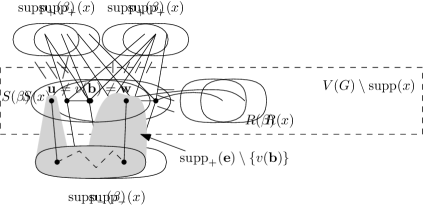
Figure 4: Connecting $f(\mathbf{u})$ and $f(\mathbf{w})$ inside $G[\operatorname{supp}_{+}(\mathbf{e})\setminus\{v(\mathbf{b})\}]$ in the case that neither $\mathbf{u}$ nor $\mathbf{w}$ belongs to $\operatorname{supp}_{-}(\beta)$.

Higher dimensions.

It remains to define $W(\mathbf{F})$ for faces $\mathbf{F}$ of $\mathbf{P}$ of higher dimensions. We inductively set $W(\mathbf{F}):=\bigcup_{\mathbf{H}}W(\mathbf{H})$, where the union is over all proper subfaces $\mathbf{H}$ of $\mathbf{F}$. As the definition is given inductively, this is equivalent with setting $W(\mathbf{F})$ to $\bigcup_{\mathbf{e}}W(\mathbf{e})$ where the union is over the edges $\mathbf{e}$ in $\mathbf{F}$. Then we easily get $f(\mathbf{F}^{(1)})\subseteq G[W(\mathbf{F})]$ for any face $\mathbf{F}$ of $\mathbf{P}$, as required.

It remains to prove that $W(\mathbf{F})$ and $W(\mathbf{F}^{\prime})$ are disjoint for any pair $\mathbf{F}$ and $\mathbf{F}^{\prime}$ of antipodal faces of $\mathbf{P}$.

For contradiction, let us assume that $W(\mathbf{F})\cap W(\mathbf{F}^{\prime})\neq\emptyset$. Due to the definition of $W(\mathbf{F})$ and $W(\mathbf{F}^{\prime})$, there are faces $\mathbf{e}$ in $\mathbf{F}$ and $\mathbf{e}^{\prime}$ in $\mathbf{F}^{\prime}$ of dimension at most 1 such that $W(\mathbf{e})\cap W(\mathbf{e}^{\prime})\neq\emptyset$. (We use the edge notation $\mathbf{e}$ and $\mathbf{e}^{\prime}$, which corresponds to the ‘typical case’; however, one of $\mathbf{e},\mathbf{e}^{\prime}$ may be a vertex, if $\mathbf{F}$ or $\mathbf{F}^{\prime}$ is $0$-dimensional.) We remark that $\mathbf{e}$ and $\mathbf{e}^{\prime}$ are antipodal as $\mathbf{F}$ and $\mathbf{F}^{\prime}$ are antipodal. Therefore, there is a proper face $\mathbf{D}$ containing $\mathbf{e}$ and $-\mathbf{e}^{\prime}$.

If neither $\mathbf{e}$ nor $\mathbf{e}^{\prime}$ is a broken edge, then $W(\mathbf{e})\subseteq\operatorname{supp}_{+}(\mathbf{e})\subseteq\operatorname{supp}_{+}(\mathbf{D})$, and $W(\mathbf{e}^{\prime})\subseteq\operatorname{supp}_{+}(\mathbf{e}^{\prime})\subseteq\operatorname{supp}_{-}(\mathbf{D})$, which is a contradiction.

Therefore, we can assume that $\mathbf{e}$ or $\mathbf{e}^{\prime}$ is a broken edge; say $\mathbf{e}^{\prime}$ is broken. Then $\mathbf{e}$ cannot be broken. (Indeed, if $\mathbf{e}$ were broken, it would have to be an edge. Therefore, by Definition 20((iv)) and Observation 17((i)), $\gamma(\mathbf{e})=\gamma(-\mathbf{e}^{\prime})$, but $\gamma(\mathbf{e}^{\prime})$ and $-\gamma(\mathbf{e}^{\prime})$ cannot be both broken due to Definition 5((ii)).) We get $W(\mathbf{e}^{\prime})\subseteq\operatorname{supp}_{+}(\mathbf{e}^{\prime})\cup\left\{v(\mathbf{e}^{\prime})\right\}\subseteq\operatorname{supp}_{-}(\mathbf{D})\cup\left\{v(\mathbf{e}^{\prime})\right\}$. On the other hand, $W(\mathbf{e})\subseteq\operatorname{supp}_{+}(\mathbf{e})\setminus\left\{v(\mathbf{e}^{\prime})\right\}\subseteq\operatorname{supp}_{+}(\mathbf{D})\setminus\left\{v(\mathbf{e}^{\prime})\right\}$. Therefore $W(\mathbf{e})$ and $W(\mathbf{e}^{\prime})$ are disjoint in this case as well. ∎

Proof of Theorem 1.

By Observation 8, $\max\left\{\lambda(G),\mu(G)\right\}\leq\eta(G)$ for every graph $G$. To prove the inequality $\eta(G)\leq\sigma(G)$, we can assume that $G$ is connected as for disconnected graphs both parameters $\eta$ and $\sigma$ are realized as the maximum of the respective parameter over the components of $G$, if it contains at least one edge (and the claim follows from the characterization of classes of graphs with $\sigma(G)\leq 0,1$ for graphs without edges; see the introduction). Applying Proposition 22 to any semivalid representation $L$ of $G$ such that $\eta(G)=\dim(L)$, we get that $\eta(G)\leq\sigma(G)$. ∎

4 On the relations between $\mu,\lambda$ and $\sigma$

In this section, we further investigate the distinction between $\mu,\lambda$ and $\sigma$. [Thm. 40]sigma proved that $\lambda(G)\leq\sigma(G)$ for every graph $G$. Moreover, [Pen98] provided an example of a graph $G$ such that $\mu(G)\leq 18$ and $\lambda(G)\geq 20$. This is the example that we mentioned in the introduction, which shows that the parameters $\sigma$ and $\mu$ are different in general.

Motivated by [Pen98, Lem. 4] establishing lower bound on $\lambda(G-e)$ for $e\in E(G)$ with special properties, we present a similar lemma for the parameter $\eta$.

Lemma 24.

Let $G=(V,E)$ be a connected graph and let $M\in\mathcal{M}(G)$. Suppose $F\subseteq E$ is such that

$$\bigcup F\cap\operatorname{supp}(x)\neq\emptyset$$

for every broken $x\in\ker(M)$ inducing more than three connected components in $G[\operatorname{supp}(x)]$. Then $\operatorname{corank}(M)-\left|F\right|\leq\eta(G)$. If, moreover, $G-F$ is connected, then $\operatorname{corank}(M)-\left|F\right|\leq\eta(G-F)$.

Proof.

Let $L:=\left\{y\in\ker(M)\colon y_{u}+y_{v}=0\ \forall uv\in F\right\}$. Clearly, $\dim(L)\geq\operatorname{corank}(M)-\left|F\right|$. We show that $L$ is a semivalid representation of $G$, and for the ‘moreover’ part, that it is also a semivalid representation of $G-F$.

To verify that $L$ is a semivalid representation of $G$, it is immediate that condition ((i)) of Definition 5 is satisfied since it holds for every nonzero vector in $\ker(M)$ (e.g., see Lemma 4((i))). Next we check condition ((ii)) of Definition 5. Assume it is not satisfied. Take a broken $y\in L$, which induces more than three connected components in $G[\operatorname{supp}(y)]$. By the assumption on $F$, there is $uv\in F$ such that $\left\{u,v\right\}\cap\operatorname{supp}(y)\neq\emptyset$. This means that $y_{u}=-y_{v}\neq 0$. However, this is impossible by Lemma 4((ii)).

Now we turn to condition ((iii)) of Definition 5. Again, we assume that the condition is not satisfied. Take $y\in L$ which has inclusion-miminal support among nonzero vectors in $L$, but at least one of the graphs $G[\operatorname{supp}_{\pm}(y)]$ is not connected. By the definition of $L$ and Lemma 4((ii)), $\bigcup F\subseteq V\setminus\operatorname{supp}(y)$. However, this means that $D:=\left\{x\in\ker(M)\colon\operatorname{supp}(x)\subseteq\operatorname{supp}(y)\right\}$ is a subspace of $L$. On the other hand, Lemma 6 says that $\dim(D)+1$ is equal to the number of connected components of $G[\operatorname{supp}(y)]$. This means that $\dim(D)\geq 2$, which implies that there is $x\in D$ with strictly smaller support than $y$; a contradiction.

Lemma 4((ii)) proves that the condition ((iv)) is satisfied as well; thus, $L$ is a semivalid representation of $G$.

To verify that $L$ is a semivalid representation of $G-F$, we first observe that if we take a nonzero $y\in L$, none of the edges $uv\in F$ can have both endpoints in $\operatorname{supp}_{+}(y)$ or $\operatorname{supp}_{-}(y)$, since $y_{u}+y_{v}=0$. Therefore, removing $F$ from $G$ cannot disconnect any of the connected components of $G[\operatorname{supp}_{+}(y)]$. Consequently, $L$ satisfies both requirements ((ii)) and ((iii)) of Definition 5 for $G-F$. Moreover, none of the edges of $uv\in F$ can have one endpoint in $\operatorname{supp}(y)$ and the other in $V\setminus\operatorname{supp}(y)$; again, because $y_{u}+y_{v}=0$. Thus, removing $F$ cannot change $N(\operatorname{supp}_{\pm}(y))$ nor $N(C)$ for any of the connected components $C$ induced by $\operatorname{supp}(y)$. Therefore, $L$ also satisfies the requirement ((iv)) of Definition 5; we conclude that $L$ is a semivalid representation of $G-F$. ∎

The next lemma is an easy consequence of Lemma 4((ii)). It generalizes [Pen98, Lem. 5].

Lemma 25.

Let $G=(V,E)$ be a connected graph with maximum degree at most $d$ and let $M\in\mathcal{M}(G)$. Let $x\in\ker(M)$ be a broken vector. Then

1. $G[\operatorname{supp}(x)]$ has at most $d$ connected components,

2. if $G[\operatorname{supp}(x)]$ has exactly $d$ connected components, then $G[V\setminus\operatorname{supp}(x)]$ has no edges and $V\setminus\operatorname{supp}(x)=N(\operatorname{supp}(x))$.

Proof.

Since $G$ is connected, Lemma 4((ii)) implies that $N(\operatorname{supp}(x))$ is nonempty, and moreover, that every vertex in $N(\operatorname{supp}(x))$ is connected to each component of $G[\operatorname{supp}(x)]$; thus, the number of such components cannot be greater than the maximum degree in $G$. This proves the first part.

For the second part, the above argument shows that $G[N(\operatorname{supp}(x))]$ does not contain any edge. Consider a vertex $v\in V\setminus\operatorname{supp}(x)\setminus N(\operatorname{supp}(x))$. Since $G$ is connected and $v\notin N(\operatorname{supp}(x))$, there must be a path from $v$ to $N(\operatorname{supp}(x))$. However, this is not possible, since all vertices in $N(\operatorname{supp}(x))$ have their neighbours only in $\operatorname{supp}(x)$. ∎

We restate here the following theorem of [Pen98, Thm. 5 ], which is very useful for proving upper bounds on $\mu(G)$.

Theorem 26 ([Pen98, Thm. 5]).

Let $G=(V,E)$ be a connected graph. Then either $G=K_{3,3}$, or $\left|E\right|\geq\binom{\mu(G)+1}{2}$.

Finite projective planes.

Let $H_{q}$ denote the incidence graph of a finite projective plane of order $q$. It is a $(q+1)$-regular bipartite graph with parts of size $q^{2}+q+1$. Using Theorem 26, this implies that

$$\mu(H_{q})\leq\left\lfloor\frac{-1+\sqrt{1+8\left|E(H_{q})\right|}}{2}\right\rfloor=\left\lfloor\frac{-1+\sqrt{1+8(q^{2}+q+1)(q+1)}}{2}\right\rfloor.$$

Let $A_{q}$ be the adjacency matrix of $H_{q}$. It is known that the spectrum of $A_{q}$ is

$$\left((q+1)^{(1)},\sqrt{q}^{(q^{2}+q)},-\sqrt{q}^{(q^{2}+q)},-(q+1)^{(1)}\right);$$

for a reference, see, e.g. [Sta17, Sec. 3.8.1, eq. (3.38)] (for that reference, note that a finite projective plane of order $q$ is a symmetric BIBD with parameters $p,b=q^{2}+q+1$, $k,r=q+1$, $\ell=1$). We further define $M_{q}:=\sqrt{q}I-A_{q}$. Clearly, $M_{q}\in\mathcal{M}(H_{q})$ and $\operatorname{corank}(M_{q})=q^{2}+q$.

Proposition 27.

$\mu(H_{3})\leq 9$ and $\sigma(H_{3})\geq 11$.

Proof.

The bound on $\mu(H_{q})$ above gives $\mu(H_{3})\leq 9$. Furthemore, $\operatorname{corank}(M_{3})=12$. Now choose any edge $e$ of $H_{3}$. Since $H_{3}$ is 4-regular, $e\cap\operatorname{supp}(x)\neq\emptyset$ for every broken $x\in\ker(M_{3})$ inducing more than three connected components in $H_{3}[\operatorname{supp}(x)]$ by Lemma 25. Thus, by Lemma 24 and Proposition 22 we see that $\sigma(H_{3})\geq\sigma(H_{3}-e)\geq\eta(H_{3}-e)\geq 11$. ∎

The separation between $\mu$ and $\sigma$ can be pushed even further by removing a small part from $H_{3}$ to obtain a graph $G$ with $\mu(G)\leq 7$ and $\sigma(G)\geq 8$, as was announced in Theorem 2 in the introduction.

Proof of Theorem 2.

We choose three vertices $v_{1},v_{2},v_{3}$ of $H_{3}$ corresponding to three points of the finite projective plane of order $3$ not lying on a single line. Let $G^{\prime}:=H_{3}-\left\{v_{1},v_{2},v_{3}\right\}$. We observe that $G^{\prime}$ contains three vertices of degree two, since every two points of a projective plane lie on a single line. Next, we choose an edge $e\in E(G^{\prime})$ adjacent to a vertex of degree three in $G^{\prime}$ and set $G:=G^{\prime}-e$.

Observe that $G$ contains four vertices of degree two; for each of these four vertices we choose one of the two edges incident to it and put it into a set $F$. We write $G/F$ for the graph resulting from a contraction of the edges of $F$ in $G$. Since a subdivision of edges preserves $\mu(H)$ for graphs $H$ with $\mu(H)\geq 3$ by [vdHLS99, Thm. 2.12], we get that $\mu(G)=\mu(G/F)$. The graph $G/F$ has $4\times 13-12-1-4=35$ edges. This means that $\mu(G)=\mu(G/F)\leq 7$ by Theorem 26. On the other hand, a removal of a vertex can decrease $\sigma$ by at most $1$ [vdHP09, Thm. 28]. As $\sigma(H_{3}-e)\geq 11$ (this was substantiated in the proof of Proposition 27 above), we deduce that $\sigma(G)\geq 8$. ∎

The proof of the following proposition is a direct generalization of the proof of [Pen98, Thm. 1].

Proposition 28.

Let $G=(V,E)$ be a connected graph of maximum degree at most $d$ and $M\in\mathcal{M}(G)$. Then $\lambda(G)\geq\operatorname{corank}(M)-d+1$.

Proof.

Let $x\in\ker(M)$ be a broken vector. The subspace

$$D(x):=\left\{y\in\ker(M)\colon\operatorname{supp}(y)\subseteq\operatorname{supp}(x)\right\}$$

has dimension at most $d-1$ by Lemma 6 and Lemma 25((i)). Let $B\subseteq\ker(M)$ be a set consisting of all broken vectors $x$ with inclusion-maximal support among broken vectors in $\ker(M)$. This implies that for every broken $y\in\ker(M)$ there is $x\in B$ such that $y\in D(x)$. Therefore, every broken vector in $\ker(M)$ is contained in a linear subspace of $\ker(M)$ of dimension at most $d-1$.

Since the number of different subsets $\operatorname{supp}(x)\subseteq V$ is finite, the number of distinct subspaces $D(x)$ for $x\in B$ is finite as well. Therefore, there is a linear subspace $L\subseteq\ker(M)$ of dimension at least $\operatorname{corank}(M)-d+1$ such that for every $x\in B$ it holds that $L\cap D(x)=\left\{\mathbf{0}\right\}$. Consequently, $L$ is a valid representation of $G$, which finishes the proof. ∎

Applying this proposition to the finite projective planes we immediately obtain an asymptotic separation of order $\mu(H_{q})\in O\left(q^{3/2}\right)$ and $\sigma(H_{q})\geq\lambda(H_{q})\geq q^{2}$, which was stated in Theorem 3 in the introduction.

Proof of Theorem 3.

Since $\operatorname{corank}(M_{q})=q^{2}+q$ and the degree of every vertex in $H_{q}$ is $q+1$, Proposition 28 implies that $\lambda(H_{q})\geq q^{2}$. The fact that $\lambda(G)\leq\sigma(G)$ for every graph $G$ was proven by [vdHP09, Thm. 40 ], as was already mentioned before.

The upper bound on $\mu(H_{q})$ follows directly from Theorem 26. ∎

Appendix A An explicit PSPACE algorithm for $\mu$

In this appendix we describe an explicit algorithm that for every graph $G=(V,E)$ on $n$ vertices and every $k\in\left\{0,\ldots,n\right\}$ decides in space polynomial in $n$ whether $\mu(G)\geq k$ or not. The strategy is to produce an existential sentence $\phi_{G,k}$ in the language $\mathfrak{L}$ of the first-order theory of the reals of length polynomial in $n$ which is true if and only if $\mu(G)\geq k$. The rest then follows by the algorithm of [Can88] for deciding the existential theory of the reals ($\exists\mathbb{R}$).

Notation.

We write $E_{i,j}$ for the matrix with one at the position $(i,j)$ and zero everywhere else. Let $G=(V,E)$ be a graph and $n:=\left|V\right|$. We write $\mathcal{O}(G)$ for the subset of $\mathbb{R}^{V\times V}$ consisting of symmetric matrices $M$ such that $M_{u,v}<0$ for every $uv\in E$ and $M_{u,v}=0$ for every $uv\notin E$. There is no requirement on the diagonal entries of $M$.

Let $p:=\binom{n}{2}-\left|E\right|$. Given a matrix $M\in\mathcal{O}(G)$, we define a $p\times n^{2}$ matrix $N(M)$ as follows: the columns of $N(M)$ consist of vectors of the form

$$\left(ME_{i,j}+E_{i,j}^{T}M\right)_{uv\notin E}$$

where $1\leq i,j\leq n$. That is, we take the matrix $ME_{i,j}+E_{i,j}^{T}M$ and turn its entries corresponding to the nonedges of $G$ into a vector (assuming some fixed ordering on the nonedges of $G$), which then constitutes a column of the matrix $N(M)$. The role of $N(M)$ will be explained below.

The definition of the parameter $\mu$ says that $\mu(G)\geq k$ if and only if there is a symmetric matrix $M\in\mathcal{O}(G)$ with exactly one negative eigenvalue and corank at least $k$ that satisfies SAH (see Subsection 2.1). It is not difficult to see that one can transfer this statement into a formula in the language $\mathfrak{L}$. Additionaly, one gets easily an $\exists\forall$-sentence of length polynomial in $n$. The reason for the presence of the universal quantifier is the definition of SAH, which is a condition on all matrices of certain form. The main ingredient in changing this formula into an existence formula is the following equivalent characterization of SAH by [Bar+17]:

Theorem 29 ([Bar+17, Thm. 31(a)]).

$M\in\mathcal{O}(G)$ satisfies SAH if and only if the matrix $N(M)$ has a full rank, i.e., its rank is $\binom{n}{2}-\left|E\right|$.

Informally, this theorem allows us to express that $M$ satisfies SAH as a formula saying ‘there is a matrix $N$ of full rank such that $N=N(M)$’. Clearly, given $M$, the matrix $N(M)$ can be constructed in time polynomial in the length of the description of $M$. In addition, we use a simple trick that enables us to prescribe the signs of the eigenvalues of $M$ and the rank of $N$; instead of searching directly for $M$ and $N$, we look for their eigendecomposition and singular value decomposition, respectively.

Proposition 30.

There is an algorithm working in time polynomial in $n$ that given as an input a graph $G=(V,E)$ with $n=\left|V\right|$ and any $k\in\left\{0,\ldots,n-1\right\}$ constructs an $\exists$-sentence $\phi=\phi_{G,k}$ in the prenex normal form in the language $\mathfrak{L}$ of size $O(n^{6})$ using $O(n^{4})$ quantified variables such that $\mu(G)\geq k$ if and only if $\phi_{G,k}$ is true.

Proof.

Let $p:=\binom{n}{2}-\left|E\right|$. The formula $\phi:=\phi_{G,k}$ will have a form equivalent to the following:

$$(\exists L,D\in\mathbb{R}^{n\times n},A\in\mathbb{R}^{p\times p},B\in\mathbb{R}^{n^{2}\times n^{2}},S\in\mathbb{R}^{p\times n^{2}})\psi(L,D,A,B,S),$$

where $\psi$ is a quantifier-free formula formed as a conjunction of polynomial equalities and inequalities with variables corresponding to entries of $L,D,A,B$ and $S$. Every element of $L,A$ and $B$ will be a real variable. On the other hand, since $D$ and $S$ will always represent diagonal matrices, only their diagonal entries will be real variables, their off-diagonal entries are always assumed to be zero.

For brevity, we write $M:=LDL^{T}$; this matrix plays the same role as in the discussions above. That is, $M$ certifies that $\mu(G)\geq k$. The matrices $L$ and $D$ represent the eigendecomposition of $M$—the matrix $D$ is a diagonal matrix with the spectrum of $M$ on its diagonal and $L$ is an orthogonal matrix representing the corresponding eigenbasis of $M$.

Similarly, we write $N:=ASB^{T}$. The matrix $N$ plays the role of $N(M)$ and $A,S,B$ represent the singular value decomposition of $N$. The singular values of $N$ are the diagonal entries of $S$ and $A,B$ are orthogonal matrices. Since the rank of $N$ is equal to the rank of $NN^{T}$ and the singular values of $N$ are the square roots of the eigenvalues of $NN^{T}$, we see that $N$ has full rank if and only if all the singular values of $N$ are positive.

The formula $\psi(L,D,A,B,S)$ is a conjunction of the formulas expressing the following:

• The formula saying that the diagonal of $D$ is

  $$(\lambda_{1},0,\ldots,0,\lambda_{k+2},\ldots,\lambda_{n}),$$

  where the number of hard-coded zero entries is $k$, together with specifying the requirements $\lambda_{1}<0$ and $\lambda_{i}\geq 0$ for $i\in\left\{k+2,\ldots,n\right\}$. This subformula has thus size only $O(n)$. Recall that $D$ is assumed to be a diagonal matrix, so its off-diagonal entries are also hard-coded to be zero (i.e., we do not need any formula to specify this).

• The formula $LL^{T}=I_{n}$. This can be written as a conjunction of $O(n^{2})$ formulas of size $O(n)$.

• The formula expressing $M\in\mathcal{O}(G)$. Clearly, this can be written as a conjunction of $O(n^{2})$ formulas, each of length $O(n)$.

• The formula saying that the diagonal of $S$ is strictly positive. This subformula has size $O(p)$, which is in $O(n^{2})$. Recall that the matrix $S$ is also assumed to be diagonal, and thus, its off-diagonal entries are hard-coded to be zero.

• The formula $A^{T}A=I_{p}$. This is a conjunction of $O(p^{2})$ formulas of size $O(p)$. In total, this is an $O(n^{6})$-long subformula.

• The formula $B^{T}B=I_{n^{2}}$. This is a subformula of size $O(n^{6})$.

• The formula saying that $ASB^{T}=N(M)$. This is a conjunction of $O(n^{4})$ formulas of length $O(n^{2})$. In total, we again have a $O(n^{6})$-long subformula.

Consequently, the size of $\phi$ is $O(n^{6})$ and it contains only one (existential) quantifier over $O(n^{4})$ variables. It is also clear that $\phi$ is constructible in time polynomial in $n$. ∎

The preceding discussion immediately implies the following corollary:

Corollary 31.

There is an explicit algorithm that computes the value of $\mu(G)$ in space polynomial in $\left|V\right|$ for any graph $G=(V,E)$.

Appendix B Recognition of graphs with $\sigma(G)\leq 5$

In this appendix, we show that $\sigma(G)>5$ can be certified in polynomial time by an explicit certificate (i.e., not via an unknown forbidden minor). We recall from the introduction that we provide here the full details in order to provide a rigorous support forthe motivation mentioned in the introduction. Otherwise, the contents of this appendix should be regarded as a basis for a future work.

Throughout Appendix B, we change our previous convention and assume that all polyhedra (and their faces) are closed.

B.1 Exponential time algorithm

First we describe the exponential time algorithm mentioned in the introduction.

Polytopal and polygonal complexes.

By a polytopal complex we mean a polyhedral complex where each polyhedron is bounded (i.e., a polytope). A polygonal complex is a polytopal comlex of dimension at most $2$.

$2$-closure.

A polygonal complex central to the contents of this section will be so called $2$-closure of a graph. Let $G=(V,E)$ be a graph. Let $\mathcal{C}_{2}(G)$ be the $2$-dimensional CW-complex obtained from $G$ by attaching a polygonal disk $D_{s}$ to every cycle $s$ in $G$. sigma define a closure of $G$ as a CW-complex $\mathcal{C}$ such that (i) $\mathcal{C}^{(1)}$ equals to $G$ and (ii) for each $i\geq 0$ and each $U\subseteq V$ that induces a connected subgraph of $G$, the higher homotopy group $\pi_{i}(\mathcal{C}^{(i+1)}[U])$ is trivial, where $\mathcal{C}[U]$ denotes the subcomplex of $\mathcal{C}$ induced by $U$. The complex $\mathcal{C}_{2}(G)$ satisfies the condition (i) and it also satisfies the condition (ii) for $i\leq 1$. From the proof of Theorem 19 in [vdHP09], it follows that $\mathcal{C}_{2}(G)$ can be extended to a closure of $G$, thus it is appropriate to call $\mathcal{C}_{2}(G)$ a $2$-closure of $G$.

It follows from [vdHP09] that $\sigma(G)\leq 5$ if and only if $\mathcal{C}_{2}(G)$ admits an even map into $\mathbb{R}^{4}$; see Proposition 32 below for precise statement convenient for our setting. As mentioned in the introduction, determining whether a $2$-complex admits an even map into $\mathbb{R}^{4}$ is known to be easy via equivariant obstruction theory (it is equivalent to vanishing of the $\mathbb{Z}_{2}$-reduction of so called van Kampen obstruction). Usually, this is set in the language of simplicial complexes but the extension to polygonal complexes is straightforward. Below we provide the details needed for explanation of our algorithm (and proof of its correctness).

Deleted product.

Given a polygonal complex $\mathcal{P}$, by $\widetilde{\mathcal{P}}$ we denote the deleted product of $\mathcal{P}$. This is the polytopal complex with faces of the form $\eta\times\tau$ where $\eta$ and $\tau$ are disjoint faces of $\mathcal{P}$. (Because of the convention for this section $\eta$ and $\tau$ are closed. Therefore their disjointness means that they do not share a vertex.) Note that $\widetilde{\mathcal{P}}$ is a $4$-dimensional complex as soon as $\mathcal{P}$ contains a pair of disjoint $2$-faces. There is a natural $\mathbb{Z}_{2}$ action on $\widetilde{\mathcal{P}}$ swapping $\eta\times\tau$ and $\tau\times\eta$.

Chains and symmetric chains.

Given a polytopal complex $\mathcal{P}$ by $C_{k}(\mathcal{P})$ we denote the space of $k$-chains of $\mathcal{P}$ (over $\mathbb{Z}_{2}$; all considerations in this section will be over $\mathbb{Z}_{2}$). This means that the elements of $C_{k}(\mathcal{P})$ are formal linear combinations

$$\sum\alpha_{\eta}\eta$$

where $\alpha_{\eta}\in\mathbb{Z}_{2}$ and the sum is over all $k$-faces $\eta$ of $\mathcal{P}$. The boundary operator $\partial\colon C_{k}(\mathcal{P})\to C_{k-1}(\mathcal{P})$ is defined so that a $k$-face $\eta$ is mapped to the sum of all $(k-1)$-faces of $\eta$ and then it is extended linearly to $C_{k}(\mathcal{P})$. An element $z\in C_{k}(\mathcal{P})$ is a $k$-cycle if $\partial z=0$. The space of $k$-cycles is denoted $Z_{k}(\mathcal{P})$. Note that we carefully distinguish graph-theoretic cycles in graph $G$ (connected subgraphs where every vertex has degree $2$) and $k$-cycles. For comparison, subgraphs of $G$ such that every vertex has even degree would be $1$-cycles in $Z_{1}(G)$, but we will never need them.

In even more special case when $\mathcal{P}=\mathcal{C}_{2}(G)$, we simplify the notation for symmetric chains in $C_{k,\mathtt{eq}}(\mathcal{C}_{2}(G))$ so that we write them in a form

$$\sum\limits\alpha_{r\times s}\cdot D_{r}\times D_{s}.$$ (1)

That is we simplify $\alpha_{D_{r}\times D_{s}}$ to $\alpha_{r\times s}$ where $r$ and $s$ are disjoint cycles of $G$. If we further set $\alpha_{\{r,s\}}:=\alpha_{r\times s}=\alpha_{s\times r}$, then (1) can be rewritten as

$$\sum\limits\alpha_{\{r,s\}}\cdot(D_{r}\times D_{s}+D_{s}\times D_{r})$$ (2)

where the sum is over all unordered pairs $\{r,s\}$ of disjoint cycles.

Symmetric cochains.

Given a polygonal complex $\mathcal{P}$, by $C^{k}_{\mathtt{eq}}(\widetilde{\mathcal{P}})$ we denote the space of corresponding symmetric cochains, that is, linear maps $m\colon C_{k,\mathtt{eq}}(\widetilde{\mathcal{P}})\to\mathbb{Z}_{2}$ satisfying $m(\eta\times\tau)=m(\tau\times\eta)$ for any $k$-face $\eta\times\tau$ of $\widetilde{\mathcal{P}}$.

General position and almost general position.

Let $\mathcal{P}$ be a polygonal complex. We say that a PL (piecewise linear) map $f\colon|\mathcal{P}|\to\mathbb{R}^{4}$ is in general position if the following two conditions are satisfied.

1. Whenever $\eta$ is an edge of $\mathcal{P}$, $x\in\eta$, $\tau$ is a $2$-face of $\mathcal{P}$, $y\in\tau$, then $f(x)=f(y)$ implies $x=y$.

2. Whenever $\eta$ and $\tau$ are distinct $2$-faces of $\mathcal{P}$, then $f(\mathrm{int}\,\sigma)$ and $f(\mathrm{int}\,\tau)$ meet in a finite number of points and each such point is a transversal crossing. (The symbol $\mathrm{int}\,$ denotes the interior.)

We say that $f$ is in almost general position if it satisfies (i) and it satisfies (ii) for every pair $\eta$ and $\tau$ of disjoint (instead of distinct) $2$-faces of $\mathcal{P}$.

Crossing cocycle.

Given a PL map $f\colon|\mathcal{P}|\to\mathbb{R}^{4}$ in almost general position, we define the crossing cocycle $\mathbf{o}_{f}\in C^{4}_{\mathtt{eq}}(\widetilde{\mathcal{P}})$ by setting $\mathbf{o}_{f}(\eta\times\tau+\tau\times\eta)$ to be the number of crossings of $f(\eta)$ and $f(\tau)$ if $\eta$ and $\tau$ are disjoint $2$-faces of $\mathcal{P}$. Then we extend $\mathbf{o}_{f}$ linearly to $C_{4,\mathtt{eq}}(\widetilde{\mathcal{P}})$. According to the definition of even map in [vdHP09], the map $f$ is even if and only if $\mathbf{o}_{f}=0$. Given $z\in Z_{4,\mathtt{eq}}(\widetilde{\mathcal{P}})$, $\mathbf{o}_{f}(z)$ coincides with $I(z,f)$ defined in [vdHP09, Sec. 4] in our special case when $f$ is an almost general position PL map. As [vdHP09] argue $I(z,f)$ is independent of the choice of $f$. Then it is possible to define $I(z)=I(z,f)$ where $f$ is an arbitrary general position PL map. Note that $I$ is a linear map from $Z_{4,\mathtt{eq}}(\widetilde{\mathcal{C}_{2}(G)})$ to $\mathbb{Z}_{2}$.

The following proposition is not explicitly mentioned in [vdHP09]. However, it immediately follows from Theorem 30 in [vdHP09] (used with $n=4$) and the equivalent definition of $\sigma$ via $I(z)$ in [vdHP09, Sec. 6].

Proposition 32 ([vdHP09]).

We get $\sigma(G)\leq 5$ if and only if $I(z)=0$ for every $z\in Z_{4,\mathtt{eq}}(\widetilde{\mathcal{C}_{2}(G)})$.

Testing $\sigma(G)\leq 5$ in exponential time.

Now we explain a simple algorithm for testing whether $\sigma(G)\leq 5$ in exponential time via Proposition 32.

Let $z^{1},\dots,z^{t}$ be a basis of $Z_{4,\mathtt{eq}}(\widetilde{\mathcal{C}(G)})$. The value $t$ as well as size of each $z^{i}$ is polynomial in the size of $\widetilde{\mathcal{C}(G)}$; however, the size of $\widetilde{\mathcal{C}(G)}$ might be (at most) exponential in size of $G$.

Because of linearity of $I$, it is sufficient to test whether $I(z^{i})=0$ for every $i\in[t]$ due to Proposition 32. Each such test can be performed in time polynomial in size of $z^{i}$. Indeed, it is sufficient to consider arbitrary general position PL map $f\colon|\mathcal{C}_{2}(G)|\to\mathbb{R}^{4}$. Then we evaluate $\mathbf{o}_{f}(z^{1}),\dots,\mathbf{o}_{f}(z^{t})$. A good particular choice when it is easy to evaluate $\mathbf{o}_{f}(z^{i})$ is to map the vertices of $G$ to the moment curve (as in [MTW11]) pick a fixed triangulation of every disk $D_{r}$ and extend the map linearly.

B.2 Speed-up

Let $n$ be the number of vertices of $G=(V,E)$, where $V=[n]$. Let $\Delta_{n-1}$ be the $n$-simplex with vertex set $V$. Note that $G$ is a subgraph of the $1$-skeleton $\Delta_{n-1}^{(1)}$. We will first define a suitable map $g\colon|\mathcal{C}_{2}(G)|\to|\Delta_{n-1}^{(2)}|$. We set $g$ as identity on $G=\mathcal{C}^{(1)}_{2}(G)$. For every cycle $r$ in $G$ we triangulate $D_{r}$ so that every triangle in the triangulation contains the minimal vertex of $r$, and we correspondingly map $D_{r}$ to $|\Delta_{n-1}^{(2)}|$, that is, a triangle in $D_{r}$ with vertices $i$, $j$, $k$ is mapped to the triangle with vertices $i$, $j$, $k$ of $\Delta_{n-1}^{(2)}$. (Note that if $r$ and $s$ are two distinct cycles of $G$, then $g(D_{r})$ and $g(D_{s})$ may easily overlap in some triangle although the disks $D_{r}$ and $D_{s}$ may overlap only on the boundary.) Note also that $g(D_{r})$ is always a disk.

Given a cycle $r$ of $G$, let $g_{\#}(D_{r})\in C_{2}(\Delta_{n-1}^{(2)})$ be the chain induced by $g$ (that is, the sum of the triangles triangulating $g(D_{r})$). Also the map $g$ induces a $\mathbb{Z}_{2}$-equivariant map $\tilde{g}\colon|\widetilde{\mathcal{C}_{2}(G)}|\to|\widetilde{\Delta_{n-1}^{(2)}}|$ given by $\tilde{g}(x,y)=(g(x),g(y))$. This map further induces an equivariant chain homomorphism $\tilde{g}_{\#,\mathtt{eq}}\colon C_{4,\mathtt{eq}}(\widetilde{\mathcal{C}_{2}(G)})\to C_{4,\mathtt{eq}}(\widetilde{\Delta_{n-1}^{(2)}})$ which we explicitly describe below.

First let us assume that $c=\tau_{1}+\dots+\tau_{k}$ and $c^{\prime}=\tau^{\prime}_{1}+\dots+\tau^{\prime}_{\ell}$ are two chains in $C_{2}(\Delta_{n-1}^{(2)})$ such that for every $i\in[k]$ and $j\in[\ell]$, $\tau_{i}$ and $\tau_{j}$ are triangles which are disjoint. Then we set $c\times c^{\prime}:=\sum_{i,j=1,1}^{k,\ell}\tau_{i}\times\tau^{\prime}_{j}$. We remark that $c\times c^{\prime}+c^{\prime}\times c$ belongs to $C_{4,\mathtt{eq}}(\widetilde{\Delta_{n-1}^{(2)}})$.

Now, given two disjoint cycles $r$ and $s$ of $G$ we set

$$\tilde{g}_{\#,\mathtt{eq}}(D_{r}\times D_{s}+D_{s}\times D_{r}):=g_{\#}(D_{r})\times g_{\#}(D_{s})+g_{\#}(D_{r})\times g_{\#}(D_{s})$$ (3)

(adapting the convention from the previous paragraph). Then we extend $\tilde{g}_{\#,\mathtt{eq}}$ linearly to $C_{4,\mathtt{eq}}(\widetilde{\mathcal{C}_{2}(G)})$. Note that the cycles $D_{r}\times D_{s}+D_{s}\times D_{r}$ generate $C_{4,\mathtt{eq}}(\widetilde{\mathcal{C}_{2}(G)})$ via (2).

Proposition 33.

Let $z$ be a symmetric $4$-cycle from $Z_{4,\mathtt{eq}}(\widetilde{\mathcal{C}_{2}(G)})$. Then $z^{\prime}=\tilde{g}_{\#,\mathtt{eq}}(z)$ is a symmetric $4$-cycle from $Z_{4,\mathtt{eq}}(\widetilde{\Delta^{(2)}_{n-1}})$. In addition, $I(z^{\prime})=I(z)$.

Proof.

First we verify that $z^{\prime}\in Z_{4,\mathtt{eq}}(\widetilde{\Delta^{(2)}_{n-1}})$. From the definition of $\tilde{g}_{\#,\mathtt{eq}}$, we get that $z^{\prime}$ belongs to $C_{4,\mathtt{eq}}(\widetilde{\Delta^{(2)}_{n-1}})$, thus we only need to verify that $z^{\prime}$ is a $4$-cycle.

Assume that

$$z=\sum\limits\alpha_{\{r,s\}}\cdot(D_{r}\times D_{s}+D_{s}\times D_{r}).$$

Then,

$$\partial z =\sum\limits\alpha_{\{r,s\}}\cdot(D_{r}\times\partial D_{s}+\partial D_{r}\times D_{s}+D_{s}\times\partial D_{r}+\partial D_{s}\times D_{r})$$

$$=\sum\limits\alpha_{\{r,s\}}\cdot(D_{r}\times s+r\times D_{s}+D_{s}\times r+s\times D_{r})$$

$$=\sum_{r}\left(D_{r}\times\left(\sum_{s}\alpha_{\{r,s\}}s\right)+\left(\sum_{s}\alpha_{\{r,s\}}s\right)\times D_{r}\right)$$

where the outer sum is over all cycles $r$ of $G$ and the inner sums are over all cycles $s$ of $G$ disjoint from $r$. Because $\partial z=0$, we get that $\sum_{s}\alpha_{\{r,s\}}s=0$ for each of the inner sums.

By analogous computation using $\partial g_{\#}(D_{r})=r$ we get

$$\partial z^{\prime} =\sum_{r}\left(g_{\#}(D_{r})\times\left(\sum_{s}\alpha_{\{r,s\}}s\right)+\left(\sum_{s}\alpha_{\{r,s\}}s\right)\times g_{\#}(D_{r})\right)$$

$$=0.$$

It remains to show $I(z)=I(z^{\prime})$. Let $f\colon|\Delta_{n-1}^{(2)}|\to\mathbb{R}^{4}$ be a general position map. Note that $f\circ g\colon|C_{2}(G)|\to\mathbb{R}^{4}$ is in almost general position. Thus, according to the definition of $I(z)$, we need to show $\mathbf{o}_{f}(z^{\prime})=\mathbf{o}_{f\circ g}(z)$.

Let $r$ and $s$ be disjoint cycles of $G$ such that $f\circ g(D_{r})$ and $f\circ g(D_{s})$ intersect in $k_{\{r,s\}}$ crossings. Then those two cycles contribute exactly by $\alpha_{\{r,s\}}k_{\{r,s\}}$ to $\mathbf{o}_{f\circ g}(z)$ (according to its definition). However, the crossings between $f\circ g(D_{r})$ and $f\circ g(D_{s})$ are also crossings of triangles in $g_{\#}(D_{r})$ and $g_{\#}(D_{s})$ when mapped under $f$. Thus they contribute by the same amount to $\mathbf{o}_{f}(z^{\prime})$ using that $z^{\prime}=\tilde{g}_{\#,\mathtt{eq}}(z)$ and formula (3). ∎

Now let $Z^{\prime}:=\tilde{g}_{\#,\mathtt{eq}}(Z_{4,\mathtt{eq}}(\widetilde{\mathcal{C}_{2}(G)}))$. According to Proposition 33, $Z^{\prime}$ is a subspace of $Z_{4,\mathtt{eq}}(\widetilde{\Delta_{n-1}^{(2)}})$.

Corollary 34.

There is $z^{\prime}\in Z^{\prime}$ with $I(z^{\prime})=1$ if and only if $\sigma(G)>5$.

Proof.

First assume that there is $z^{\prime}\in Z^{\prime}$ with $I(z^{\prime})=1$. Then there is also $z\in Z_{4,\mathtt{eq}}(\widetilde{\mathcal{C}_{2}(G)})$ such that $z^{\prime}=\tilde{g}_{\#,\mathtt{eq}}(z)$. According to Proposition 33, $I(z)=1$. Therefore $\sigma(G)>5$ by Proposition 32.

On the other hand, let us assume that $\sigma(G)>5$. Then there is $z\in Z_{4,\mathtt{eq}}(\widetilde{\mathcal{C}_{2}(G)})$ with $I(z)=1$ by Proposition 32. Then $\tilde{g}_{\#,\mathtt{eq}}(z)$ is the required $z^{\prime}$ by Proposition 33. ∎

Theorem 35.

For any graph $G$, there is an explicit polynomial size certificate showing $\sigma(G)>5$.

Proof.

By Corollary 34, it is sufficient to certificate an existence of $z^{\prime}\in Z^{\prime}$ with $I(z^{\prime})=1$. We can easily observe that the dimension of $Z^{\prime}$ is polynomially bounded by the size of $G$ because $Z^{\prime}$ is a subspace of $C_{4,\mathtt{eq}}(\widetilde{\Delta^{(2)}_{n-1}})$. A safe bound is that $C_{4,\mathtt{eq}}(\widetilde{\Delta^{(2)}_{n-1}})$ is generated by at most $\binom{n}{3}^{2}$ pairs of triangles where $n$ is the number of vertices of $G$. Therefore, there is a chain $z\in Z_{4,\mathtt{eq}}(\widetilde{\mathcal{C}_{2}(G)})$ with polynomially many nonzero coordinates satisfying $z^{\prime}=\tilde{g}_{\#,\mathtt{eq}}(z)$ which thereby certifies that $z^{\prime}\in Z$. Certifying $I(z^{\prime})=1$ is easy via a suitable general position map (as described for the exponential time algorithm). ∎

Remark 36.

If we knew how to find a basis of $Z^{\prime}$ in polynomial time, then we would immediately get a polynomial time algorithm by evaluating $I(z^{\prime})$ for all basis cycles $z^{\prime}$.

References

- [BC95] R. Bacher and Y. Colin de Verdière “Multiplicités des valeurs propres et transformations étoile-triangle des graphes” In Bulletin de la Société Mathématique de France 123.4 Société mathématique de France, 1995, pp. 517–533 DOI: 10.24033/bsmf.2269
- [Bar+17] W. Barrett et al. “Generalizations of the Strong Arnold Property and the Minimum Number of Distinct Eigenvalues of a Graph” In Electr. J. Comb. 24, 2017, pp. P2.40 URL: https://bit.ly/32qqM9D
- [Can88] J. Canny “Some Algebraic and Geometric Computations in PSPACE” In Proceedings of the Twentieth Annual ACM Symposium on Theory of Computing, STOC ’88 New York, NY, USA: ACM, 1988, pp. 460–467 DOI: 10.1145/62212.62257
- [Col90] Y. Colin de Verdière “Sur un nouvel invariant des graphes et un critère de planarité” In Journal of Combinatorial Theory, Series B 50.1, 1990, pp. 11–21 DOI: 10.1016/0095-8956(90)90093-F
- [Col91] Y. Colin de Verdière “On a new graph invariant and a criterion for planarity.” In Graph Structure Theory 147, Contemporary Mathematics American Mathematical Society, 1991, pp. 137–147 DOI: 10.1090/conm/147
- [DW13] V. Dujmović and S. Whitesides “Three-Dimensional Drawings” In Handbook of Graph Drawing and Visualization, Discrete Mathematics and Its Applications CRC Press, 2013 DOI: 10.1201/b15385
- [ES74] G. Ewald and G.. Shephard “Stellar subdivisions of boundary complexes of convex polytopes” In Math. Ann. 210, 1974, pp. 7–16 DOI: 10.1007/BF01344542
- [Foi03] J. Foisy “A newly recognized intrinsically knotted graph” In J. Graph Theory 43.3, 2003, pp. 199–209 DOI: 10.1002/jgt.10114
- [Gol13] F. Goldberg “Optimizing Colin de Verdière matrices of ” Special issue in honor of Abraham Berman, Moshe Goldberg, and Raphael Loewy In Linear Algebra and its Applications 438.10, 2013, pp. 4090–4101 DOI: 10.1016/j.laa.2012.09.006
- [vdHol95] H. Holst “A Short Proof of the Planarity Characterization of Colin de Verdière” In Journal of Combinatorial Theory, Series B 65.2, 1995, pp. 269–272 DOI: 10.1006/jctb.1995.1054
- [vdHLS95] H. Holst, M. Laurent and A. Schrijver “On a Minor-Monotone Graph Invariant” In Journal of Combinatorial Theory, Series B 65.2, 1995, pp. 291–304 DOI: 10.1006/jctb.1995.1056
- [vdHLS95a] H. Holst, L. Lovász and A. Schrijver “On the invariance of Colin de Verdière’s graph parameter under clique sums” Honoring J. J. Seidel In Linear Algebra and its Applications 226-228, 1995, pp. 509–517 DOI: 10.1016/0024-3795(95)00160-S
- [vdHLS99] H. Holst, L. Lovász and A. Schrijver “The Colin de Verdière graph parameter” In Graph Theory and Combinatorial Biology, Bolyai Society Mathematical Studies Hungary: János Bolyai Mathematical Society, 1999, pp. 29–85 URL: https://bit.ly/2OWRMd6
- [vdHP09] H. Holst and R. Pendavingh “On a graph property generalizing planarity and flatness” In Combinatorica 29.3, 2009, pp. 337–361 DOI: 10.1007/s00493-009-2219-6
- [Izm10] I. Izmestiev “The Colin de Verdière number and graphs of polytopes” In Israel Journal of Mathematics 178.1, 2010, pp. 427–444 DOI: 10.1007/s11856-010-0070-5
- [KT20] V. Kaluža and M. Tancer “Even maps, the Colin de Verdière number and representations of graphs” In Proceedings of the 2020 ACM-SIAM Symposium on Discrete Algorithms, 2020, pp. 2642–2657 DOI: 10.1137/1.9781611975994.161
- [KLV97] A. Kotlov, L. Lovász and S. Vempala “The Colin de Verdière number and sphere representations of a graph” In Combinatorica 17.4, 1997, pp. 483–521 DOI: 10.1007/BF01195002
- [Lov01] L. Lovász “Steinitz Representations of Polyhedra and the Colin de Verdière Number” In Journal of Combinatorial Theory, Series B 82.2, 2001, pp. 223–236 DOI: 10.1006/jctb.2000.2027
- [LS98] L. Lovász and A. Schrijver “A Borsuk theorem for antipodal links and a spectral characterization of linklessly embeddable graphs” In Proceedings of the American Mathematical Society 126.5 American Mathematical Society, 1998, pp. 1275–1285 DOI: 10.1090/S0002-9939-98-04244-0
- [LS99] L. Lovász and A. Schrijver “On the null space of a Colin de Verdière matrix” In Annales de l’Institut Fourier 49.3 Association des Annales de l’institut Fourier, 1999, pp. 1017–1026 DOI: 10.5802/aif.1703
- [MTW11] J. Matoušek, M. Tancer and U. Wagner “Hardness of embedding simplicial complexes in ” In J. Eur. Math. Soc. (JEMS) 13.2, 2011, pp. 259–295 DOI: 10.4171/JEMS/252
- [McC18] R. McCarty “The Extremal Function and Colin de Verdière Graph Parameter” In Electronic Journal of Combinatorics 25(2), 2018, pp. P2.32 URL: https://bit.ly/2OYCQLI
- [McC19] R.. McCarty Personal communication, 2019
- [Pen98] R. Pendavingh “On the Relation Between Two Minor-Monotone Graph Parameters” In Combinatorica 18.2, 1998, pp. 281–292 DOI: 10.1007/PL00009821
- [RS95] N. Robertson and P.. Seymour “Graph minors. XIII. The disjoint paths problem” In J. Combin. Theory Ser. B 63.1, 1995, pp. 65–110 DOI: 10.1006/jctb.1995.1006
- [RS04] N. Robertson and P.. Seymour “Graph minors. XX. Wagner’s conjecture” In J. Combin. Theory Ser. B 92.2, 2004, pp. 325–357 DOI: 10.1016/j.jctb.2004.08.001
- [RST95] N. Robertson, P. Seymour and R. Thomas “Sachs’ Linkless Embedding Conjecture” In Journal of Combinatorial Theory, Series B 64.2, 1995, pp. 185–227 DOI: 10.1006/jctb.1995.1032
- [RS82] C.. Rourke and B.. Sanderson “Introduction to piecewise-linear topology” Reprint, Springer Study Edition Springer-Verlag, Berlin-New York, 1982 DOI: 10.1007/978-3-642-81735-9
- [Sch13] M. Schaefer “Hanani-Tutte and related results” In Geometry—intuitive, discrete, and convex 24, Bolyai Soc. Math. Stud. János Bolyai Math. Soc., Budapest, 2013, pp. 259–299 DOI: 10.1007/978-3-642-41498-5˙10
- [SS17] A. Schrijver and B. Sevenster “The Strong Arnold Property for 4-connected flat graphs” In Linear Algebra and its Applications 522, 2017, pp. 153–160 DOI: 10.1016/j.laa.2017.02.002
- [Sta17] Z. Stanić “Regular Graphs: A Spectral Approach”, De Gruyter Series in Discrete Mathematics and Applications De Gruyter, 2017 DOI: 10.1515/9783110351347
- [Sti04] D.. Stinson “Combinatorial Designs: Construction and Analysis” Springer-Verlag New York, 2004 DOI: 10.1007/B97564
- [Tai19] M. Tait “The Colin de Verdière parameter, excluded minors, and the spectral radius” In Journal of Combinatorial Theory, Series A 166, 2019, pp. 42–58 DOI: 10.1016/j.jcta.2019.02.018
- [TT13] M. Tancer and D. Tonkonog “Nerves of good covers are algorithmically unrecognizable” In SIAM J. Comput. 42.4, 2013, pp. 1697–1719 DOI: 10.1137/120891204
- [Tho99] R. Thomas “Recent Excluded Minor Theorems for Graphs” In Surveys in Combinatorics, 1999, London Mathematical Society Lecture Note Series Cambridge University Press, 1999, pp. 201–222 DOI: 10.1017/CBO9780511721335.008
- [Zie95] G.. Ziegler “Lectures on polytopes” 152, Graduate Texts in Mathematics Springer-Verlag, New York, 1995 DOI: 10.1007/978-1-4613-8431-1