Proportional Dynamics in Exchange Economies

Abstract.

We study the proportional dynamics in exchange economies, where each player starts with some amount of money and a good. Every day, players bring one unit of their good and submit bids on goods they like, each good gets allocated in proportion to the bid amounts, and each seller collects the bids received. Then every player updates their bids proportionally to the contribution of each good in their utility.

This dynamic models a process of learning how to bid and has been studied in a series of papers on Fisher and production markets, but not in exchange economies. Our main results are as follows:

1. For all linear utilities, the dynamic converges to market equilibrium utilities and allocations, while the bids and prices may cycle. We give a combinatorial characterization of limit cycles for prices and bids.

2. We introduce a lazy version of the dynamic, where players may save money for later, and show this converges in everything: utilities, allocations, and prices.

This answers an open question about exchange markets with linear utilities, where tâtonnement does not converge to market equilibria, and no natural process leading to equilibria was known for all additive utilities. We also note this dynamics represents a process where the players exchange goods throughout time (in out-of-equilibrium states), while tâtonnement only explains how exchange happens in the limit.

<ccs2012> <concept> <concept_id>10003752.10010070.10010099</concept_id> <concept_desc>Theory of computation Algorithmic game theory and mechanism design</concept_desc> <concept_significance>500</concept_significance> </concept> <concept> <concept_id>10003752.10010070.10010099.10010105</concept_id> <concept_desc>Theory of computation Convergence and learning in games</concept_desc> <concept_significance>500</concept_significance> </concept> <concept> <concept_id>10003752.10010070.10010099.10010106</concept_id> <concept_desc>Theory of computation Market equilibria</concept_desc> <concept_significance>500</concept_significance> </concept> <concept> <concept_id>10003752.10010070.10010099.10010109</concept_id> <concept_desc>Theory of computation Network games</concept_desc> <concept_significance>500</concept_significance> </concept> </ccs2012>

[500]Theory of computation Algorithmic game theory and mechanism design [500]Theory of computation Convergence and learning in games [500]Theory of computation Market equilibria [500]Theory of computation Network games

1. Introduction

Market dynamics have been an integral part of general equilibrium theory since its inception. The introduction of general equilibrium theory by Walras Walras (1896) was accompanied by the idea of the tâtonnement process. Fisher designed in 1891 a device to compute an equilibrium (Brainard and Scarf Brainard and Scarf (2005)). The most popular interpretation of tâtonnement, however, is as fictitious play. An auctioneer, playing the role of the invisible hand, calls out prices to which the agents respond with their demand, then the auctioneer adjusts the prices, and the process repeats until the excess demand is zero. At this point exchange actually happens, at equilibrium prices. This, however, is not necessarily how actual markets function in practice. Moreover, general equilibrium theory itself suffers from a lack of a descriptive model of out of equilibrium exchange: what happens when the excess demand is positive? Further, the causal linkage between demand and prices is unspecified. Demand is a response to the price as well as the price is a response to the demand. (See Fisher (1983) for some disequilibrium extensions; there is no widely agreed upon model.) The question is fundamentally both algorithmic and economic. Algorithmically, the question is about an effective and efficient locally controlled network process that computes an equilibrium. Economically, the question is about an incentives-motivated multi-agent process that converges to equilibrium.

Shapley and Shubik Shapley and Shubik (1977) sought to address these issues via the trading post mechanism. This is first of all a descriptive model that specifies concrete outcomes as a result of player strategies, and therefore it can be viewed as a non-cooperative game. Prices are a result of strategic actions; the higher the demand for a good, the higher its price, and vice versa. It requires that all trade be monetary and that the players pay cash in advance. Each player submits a cash bid on each good. The goods are then distributed in proportion to the bids, and the per-unit price of a good is set to be the sum of bids on that good (this implies that the bids of a player should add up to at most the cash at hand). The same mechanism has been rediscovered multiple times; in particular it has been proposed for sharing resources in computer networks (e.g. Kelly Kelly (1997)) and computer systems (e.g. Feldman, Lai, and Zhang Feldman et al. (2005)).

This still leaves open the question of dynamics: (how) do players reach a market equilibrium in the trading post mechanism? The predominant answer to this in the last decade or so has been the proportional response dynamic (see Zhang Zhang (2011)), where buyers iteratively update their bid on each good in proportion to the utility they received from that good in the previous iteration. For the case of linear utilities, this implies that the ratio of bids in successive iterations is proportional to the bang-per-buck for that good, in contrast to the best response which distributes all the cash among the goods with the highest bang-per-buck. Such an update is similar in spirit to the multiplicative weights update algorithms used in online learning (also to proportional tâtonnement), except that there are no parameters such as the step size to tune carefully! It still magically seems to work. Wu and Zhang Wu and Zhang (2007) studied a dynamic without money, in a special type of exchange market, where each good has a common value (i.e. the value of any good $j$ is the same for every player $i$: $v_{i,j}=v_{j}$), and showed it converges to market equilibria.

1.1. Our results

This brings us to the topic of this paper, the study of proportional response dynamics in exchange markets. The players are both buyers and sellers, and the exchange at each step is fueled by the players revenue from the previous round, and a fresh batch of goods of fixed quantities at the hands of the players. We focus primarily on linear utilities. Linear utilities are a widely studied type of utility that are also of interest because the process of tâtonnement is not well defined in markets with such utilities. Tâtonnement adjusts the prices based on the excess demand for a good, but with linear utilities the demand is a set function. Also, the demand is discontinuous: a small change in price can lead to a large change in demand. This makes tâtonnement especially unsuited as a process describing market dynamics for linear utilities. In contrast, linear utilities pose no such problem for proportional response dynamics. For complements, especially in the extreme case of Leontief utilities, there is scant hope for fast convergence since computationally the problem of finding an equilibrium is PPAD-hard (see Codenotti, Saberi, Varadarajan, and Ye Codenotti et al. (2006)). However this does not rule out the existence of a slowly converging process.

The dearth of convergence results in this setting is not for the lack of trying (see, e.g., gradient descent based algorithms Chen et al. (2019)). The difficulty might be attributed to the fact that the dynamics can cycle! Consider the scenario where there are two sets of players such that each set buys all its goods from the other set. Suppose that the sets start with widely unequal amounts of cash. Then in each iteration, the total amount of cash of each set moves to the other side, forever. However there is still hope: the allocations and the utilities of the players could converge to those of a market equilibrium, even if the prices oscillate. (In fact, in the above example the relative prices in each set may converge, even though the price scales alternate between the sides.)

We study the exchange economy model, where each player comes to the market with a unit endowment of an exclusive good. For linear utilities, this model is without loss of generality for the equilibrium computation problem, as there is a reduction from the general model, where each player can bring multiple goods, to the one where each player brings only one good. We The equilibrium utilities are unique, while the equilibrium allocation may not be. Our main results are as follows:

1. We show that the kind of cycling described above is essentially the only one possible. We characterize the limit cycles of the dynamics as follows: there are equivalence classes of players such that within each class the ratio of price to equilibrium price is a constant. Further, the classes form a cycle, where the players in each class only buy goods from the players in the next class in the cycle. The allocations and utilities correspond to a market equilibrium, and remain invariant all along the limit cycle. (Theorem 4.24)

2. We show that the allocation and hence the utilities converge (Theorem 4.20). The result in the previous item only shows that the limit set in the allocation space is the set of equilibrium allocations. Convergence to this set is implied.

3. We introduce a lazy version  of the proportional response dynamics, where players saves a certain fraction of their cash at hand for future rounds (Definition 2). The fraction can be different for each player, as long as it is in $(0,1)$, but it doesn’t change over time. We show that for this version, there is no cycling: prices, allocation and utilities all converge to a market equilibrium (Theorem 3.13).

4. We also prove an ergodic rate of convergence of $O(1/T)$ for the utilities, with respect to the Eisenberg-Gale objective function, which captures the market equilibrium allocations and utilities. We note that our simulations indicate that the last iterate also converges, and that the convergence rate is much faster than proved.

1.2. Previous work

Most of the results for the convergence of the proportional response dynamics to date have been for Fisher markets, where the players act as buyers, and each step is fueled by a fixed income of each player and a fresh batch of goods. Zhang Zhang (2011) shows convergence of proportional response dynamics to the market equilibrium for Constant Elasticity of Substitution (CES) utilities in the substitutes regime. Birnbaum, Devanur, and Xiao Birnbaum et al. (2011) interpret proportional as mirror descent on the convex program of Shmyrev Shmyrev (2009) that captures equilibria in Fisher markets with linear utilities, and also extends it to some other markets. Cheung, Cole, and Tao Cheung et al. (2018) extend the approach in Birnbaum et al. (2011) to show that proportional response converges for the entire range of CES utilities including complements, with linear utilities on one extreme and Leontief utilities on the other extreme. Cheung, Hoefer, and Nakhe Cheung et al. (2019b) show that the dynamics stays close to equilibrium even when the market parameters are changing slowly over time, once again for CES utilities.

Wu and Zhang Wu and Zhang (2007) also study a dynamics in an exchange setting. The Wu-Zhang dynamic is different from the one we study because it does not use money and converges only in the special case of the exchange market where each good has a common value (i.e. where the value of each player $i$ for each good $J$ is $v_{i,j}=v_{j}$). The Wu-Zhang dynamics is motivated by application of exchange from networking, where it is preferable to not use money. We note that the dynamics in our paper is the correct generalization of proportional response as it was studied for Fisher markets (see Zhang Zhang (2011) and Birnaum-Devanur-XiaoBirnbaum et al. (2011)). We also show that the dynamics from  Wu and Zhang (2007) and our proportional response dynamics are functionally different, i.e. they have different trajectories in terms of allocations and utilities, even in the special case of the market where goods have common values and given the same starting configurations. In fact, when the goods do not have a common value (i.e. the players can value different goods differently), we find an example of a market linear where the Wu-Zhang dynamics cycles (see Appendix 5).

Branzei, Mehta, and Nisan Branzei et al. (2018) generalized the definition of proportional response from Fisher markets to an exchange setting with production. The definition of proportional response in Branzei et al. (2018) is the same as the one we use, except the amounts are fixed over time in our model. On the other hand, in the production market, players make new goods from the ones they acquire through the trading post mechanism, and the new goods are sold in the next iteration. There, the proportional response dynamics leads to growth of the market, i.e. the amount of goods produced grow over time, but also to growing inequality between the players on the most efficient production cycles and the rest.

The study of convergence of tâtonnement goes back at least as far as Arrow, Block, and Hurwicz Arrow et al. (1959), which was soon followed by examples of cycling (see Scarf Scarf (1960) and Gale Gale (1963)). For markets with weak gross substitutes utilities (WGS), a polynomial time convergence of a discrete time process was shown by Codenotti, McCune, and Varadarajan Codenotti et al. (2005a), and Cole and Fleischer Cole and Fleischer (2008) showed fast convergence not just for static markets, but also “ongoing” markets. (See also Fleischer, Garg, Kapoor, Khandekar, and Saberi Fleischer et al. (2008).) This was followed up by similar analysis for some markets with complementarities (Cheung, Cole, and Rastogi Cheung et al. (2012); Cheung and Cole Cheung and Cole (2014); Avigdor, Rabani, and Yadgar Avigdor-Elgrabli et al. (2014)), then for all “Eisenberg-Gale” markets in the Fisher model Cheung et al. (2019a). Some of these analyses apply to ongoing and/or asynchronous settings.

Several approaches have been explored for the (centralized) computation of equilibria in a linear exchange market: the ellipsoid method (Jain Jain (2007); Codenotti, Pemmaraju, and Varadarajan Codenotti et al. (2005b)), interior point algorithms (Ye Ye (2008)), combinatorial flow based methods (Jain, Mahdian, and Saberi Jain et al. (2003); Devanur and Vazirani  Devanur and Vazirani (2003); Duan and Mehlhorn Duan and Mehlhorn (2015); Duan, Garg, and Mehlhorn Duan et al. (2016)). Extending the Fisher market version of Devanur et al. (2008)) recently led to a strongly polynomial time algorithm (Garg and Végh Garg and Végh (2019)). Other approaches include auction based algorithms Garg and Kapoor (2006); Bei et al. (2019), cell decomposition Deng et al. (2003); Devanur and Kannan (2008), complementary pivoting Garg et al. (2015), and computational versions of Sperner’s lemma Echenique and Wierman (2011); Scarf (1977). On the other hand, computing an equilibrium with even the simplest kind of complementarities is PPAD-hard Codenotti et al. (2006); Chen et al. (2009).

There has been extensive work on understanding dynamics in games and auction settings under various behavioural models of the agents, such as best-response dynamics, multiplicative weight updates, fictitious play (e.g., Freund and Schapire (1999); Kleinberg et al. (2009); Daskalakis et al. (2015); Mehta et al. (2015); Panageas and Piliouras (2016); Roughgarden et al. (2017); Daskalakis and Syrgkanis (2016); Hassidim et al. (2011); Papadimitriou and Piliouras (2016); Lykouris et al. (2016)) and best response processes and other dynamics of learning how to bid in market settings Chen and Deng (2011); Nisan et al. (2011); Bhawalkar and Roughgarden (2011); Lucier and Borodin (2010); Babaioff et al. (2017); Dütting and Kesselheim (2017); Cary et al. (2014); Branzei and Filos-Ratsikas (2019)). In the former the focus has been on convergence to an equilibrium, preferable Nash, and if not then (coarse) correlated equilibria, and the rate of covergence. In the latter the focus has been on either convergence points and their quality (price-of-anarchy), or dynamic mechanisms such as ascending price auctions to reach efficient allocations (e.g. the Ausubel auction Ausubel (2004)).

1.3. Difficulties and techniques

The strongest convergence results for proportional response dynamics in Fisher markets are achieved via the mirror descent interpretation on suitable convex programs Birnbaum et al. (2011); Cheung et al. (2018). Devanur, Garg, and Végh Devanur et al. (2016) show a similar (but more complicated) convex program for linear utilities in exchange markets. It is therefore tempting to conjecture that a similar mirror descent interpretation would extend to exchange markets as well, but unfortunately this doesn’t seem to be the case. There are many difficulties, but the easiest to explain is the following. In the Fisher case, the proportional response bids are by definition in the feasible region of the convex program, which asks that the price of a good equal the total bids placed on it, and that the budget of a player equal the total of his own bids. In the exchange case, the price of a good is still the total bid placed on it by definition, but the total bid a player issues equals his earnings from the previous iteration, which may differ from the total bid placed on its good in the current iteration. The convex program requires these equality constraints, so the bids don’t stay inside the feasible region as in the Fisher case.

We use the KL divergence between equilibrium bids and the current bids as a Lyapunov function; this divergence was also used in Zhang (2011) when analyzing Fisher markets. The convergence of utilities is the easiest, and follows almost exactly the analysis for Fisher markets. Beyond utilities, the cycling of bids presents more difficulties. We characterize the limit cycles by considering the zero set of a certain set of equations. We argue that their structure is like that of the price ratios in the limit cycles described above. The convergence of allocation follows from showing that the KL divergence between the (equilibrium and current) bids can be decomposed into a positive linear combination of the KL divergence between the prices and the KL divergences between the allocations for each good. This also implies that the KL divergence between equilibrium prices and prices on a limit cycle must be an invariant.

For the lazy version we show that adding a suitably weighted KL divergence between equlibrium prices and current budgets to the Lyapunov function does the trick. This collapses the limit cycles so that the limit set becomes just the equilibria. This then gives us that the Lyapunov function must go to zero, which implies convergence of prices as well.

1.4. Organization of the paper

In Section 2, we give the definitions of the two variants of the proportional response dynamics, and market equilibria and state some useful properties. We also show numeric examples of cycling for the non-lazy version. Section 3 defines a Lyapunov function for the dynamics, which shows convergence of utilities. We also show convergence of allocation and prices for the strictly lazy version. In Section 4, we characterize limit cycles, and show convergence of allocation for the non-lazy version. Section 5 shows a comparison with the tit-for-tat dynamic, including an example where tit-for-tat cycles. We can conclude with a discussion in Section 6.

2. Preliminaries

There are $n$ agents, each of which has one unit of an eponymous good. The goods are divisible. The agents have linear utilities given by a matrix $A=\{a_{i,j}\}$, where $a_{i,j}\geq 0$ is the valuation of agent $i$ for one unit of the good owned by agent $j$. We assume that every agent has a certain quantity of a numeraire to start with, which we call money. All the prices will be determined in terms of this numeraire. The agents don’t have any utility for the money; it just facilitates exchange of goods.

The assumption on the valuations $a_{i,j}$ will be that a market equilibrium exists for the induced exchange market. An equilibrium does not exist when some agent has no edges; in some sense such agents do not participate in the economy and will not be considered in the dynamics.

2.1. Proportional Response Dynamics in Exchange Economies:

The proportional response dynamics describes a process in which the players come to the market every day with one unit of good and some budget, which is split into bids. The players bid on the goods, then the seller of each good allocates it in proportion to the bid amounts and collects the money from selling, which becomes its budget in the next round. Finally the players update their bids in proportion to the contribution of each good to their utility.

Definition 1 (Proportional Response Dynamics).

The initial bids of player $i$ are $b_{i,j}(0)$, which are non-zero whenever $a_{i,j}>0$. Then, at each time $t$, the following steps occur:

Exchange of goods:

Each player $i$ brings one unit of its good and submits bids $b_{i,j}(t)$. The player receives an amount $x_{i,j}(t)$ of each good $j$, where

$$x_{i,j}(t)=\left\{\begin{array}[]{ll}\frac{b_{i,j}(t)}{\sum_{k=1}^{n}b_{k,j}(t)},&\mbox{if}\;b_{i,j}(t)>0\\ 0,&\mbox{otherwise}\end{array}\right.$$

Each player $i$ computes the utility for the bundle acquired: $u_{i}(t)=\sum_{j=1}^{n}a_{i,j}\cdot x_{i,j}(t)\,.$

Bid update:

Each player $i$ collects the money made from selling: $B_{i}(t+1)=\sum_{k=1}^{n}b_{k,i}(t)$ and updates his bids proportionally to the contribution of each good in his utility:

$$\textstyle b_{i,j}(t+1)=\left(\frac{a_{i,j}\cdot x_{i,j}(t)}{u_{i}(t)}\right)\cdot B_{i}(t+1)\,.$$

Normalization: Without loss of generality, we can assume the total amount of money in the economy is $1$.

Remark 1.

The sum of bids on a good can be seen as its price, so we will write $p_{i}(t)=\sum_{k=1}^{n}b_{k,i}(t)\,.$

The next figure shows an instance with twelve players. The allocations, utilities, and prices oscillate initially but stabilize later.

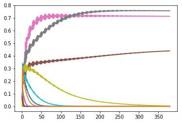
(a) Allocations $x_{i,j}(t)$ over time.

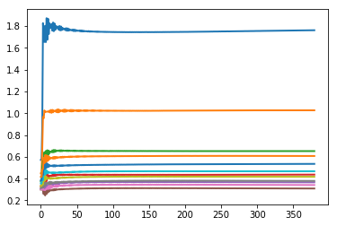
(b) Utilities $u_{i}(t)$ over time.

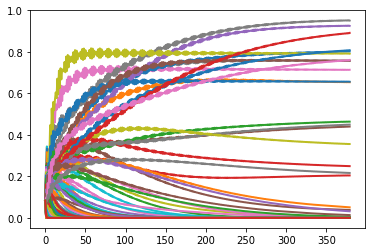
(c) Bids $b_{i,j}(t)$ over time.

Figure 1. Proportional response dynamics in an economy with $n=12$ players over $T=380$ rounds: allocations, utilities, and bids.

Figure 2 shows an example trajectory in a ten player economy. In this example it can be seen that the allocations and utilities converge while the prices cycle.

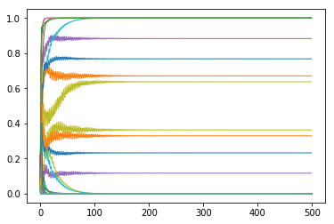
(a) Allocations $x_{i,j}(t)$ over time.

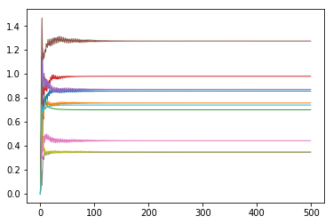
(b) Utilities $u_{i}(t)$ over time.

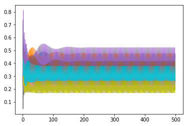
(c) Prices $p_{i}(t)$ over time.

Figure 2. Proportional response dynamics in an economy with $n=10$ players over $T=500$ rounds: allocations, utilities, and prices. The set of players is divided in three groups: $\left(C_{1},C_{2},C_{3}\right)$, where $C_{4}=C_{1}$, $C_{1}=\{1,2,3\}$, $C_{2}=\{4,5,6,7\}$, and $C_{3}=\{8,9,10\}$. The valuations are such that the players in group $C_{i}$ only value the goods of players in group $C_{i+1}$.

2.2. Lazy Proportional Response Dynamics in Exchange Economies:

Our first contribution is to define a more general framework for the proportional response dynamics, which can be seen as a lazy version of the dynamic. Each player will spend only some fraction $\alpha_{i}\in(0,1]$ of its total money in each round, while saving the remaining fraction of $1-\alpha_{i}$ in the bank. Then in the next round, the player collects the money it made from selling and takes out the money from the bank, which sum up to its total amount of money. Then again the player spends a fraction $\alpha_{i}$ of its total money, while saving the remainder of $1-\alpha_{i}$ in the bank.

Formally, we have the following definition.

Definition 2 (Lazy Proportional Response Dynamics).

Initially each player $i$ has some amount of money $m_{i}(0)$. The player splits a fraction $\alpha_{i}\in(0,1]$ of the money into initial bids $b_{i,j}(0)$, which are non-zero whenever $a_{i,j}>0$. I.e., the budget for spending at time $0$, which is $B_{i}(0)\triangleq\alpha_{i}\cdot m_{i}(0)$, is split into bids $b_{i,j}(0)$ satisfying $\sum_{j}b_{i,j}(0)=\alpha_{i}\cdot m_{i}(0)$, and the player saves the remaining portion of money $(1-\alpha_{i})\cdot m_{i}(0)$ in the bank.

At each time $t$, the next steps take place:

Exchange of goods:

Each player $i$ brings one unit of its good and submits bids $b_{i,j}(t)$. The player receives an amount $x_{i,j}(t)$ of each good $j$, where

$$x_{i,j}(t)=\left\{\begin{array}[]{ll}\frac{b_{i,j}(t)}{\sum_{k=1}^{n}b_{k,j}(t)},&\mbox{if}\;b_{i,j}(t)>0\\ 0,&\mbox{otherwise}\end{array}\right.$$

Each player $i$ computes the utility for the bundle acquired: $u_{i}(t)=\sum_{j=1}^{n}a_{i,j}\cdot x_{i,j}(t).$

Bid update:

Each player $i$ collects the money made from selling: $p_{i}(t)=\sum_{k=1}^{n}b_{k,i}(t)$.

The total money of player $i$ is the price of the good sold plus the money saved: $m_{i}(t+1)=p_{i}(t)+(1-\alpha_{i})B_{i}(t)/\alpha_{i}$. This gets split again into a fraction of $(1-\alpha_{i})$, saved in the bank, and a fraction $\alpha_{i}$ that will be spent in the next round: $\textstyle B_{i}(t+1)=\alpha_{i}\cdot m_{i}(t+1)=\alpha_{i}\cdot p_{i}(t)+(1-\alpha_{i})B_{i}(t).$

The player updates his bids proportionally to the contribution of each good in his utility:

$$\textstyle b_{i,j}(t+1)=\left(\frac{a_{i,j}\cdot x_{i,j}(t)}{u_{i}(t)}\right)\cdot B_{i}(t+1)$$

Notice that the special case of this dynamic where $\alpha_{i}=1$ for all agents $i$ is simply the proportional response dynamic of Definition 1.

In Figure 3 we show the dynamics for the same valuations and initial bids as in Figure 2, but where the players save half of their money in the bank at each time unit.

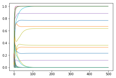
(a) Allocations $x_{i,j}(t)$ over time.

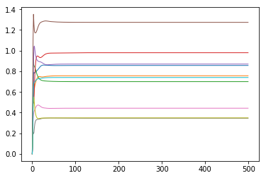
(b) Utilities $u_{i}(t)$ over time.

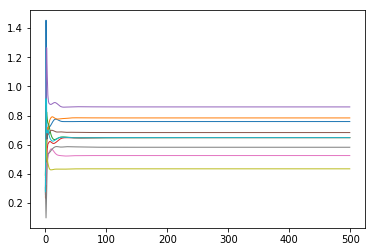
(c) Prices $p_{i}(t)$ over time.

Figure 3. Lazy version of the dynamics where the players have the same valuations and initial budgets and bids as in Figure 2, but they also have a matching amount saved in the bank, and in each round they save $50\%$ of their money.

2.3. Market Equilibria

We review the definition of market equilibria and some useful properties. We assume that for each good $j$ there is at least one player $i$ such that $a_{i,j}>0$. An equilibrium is given by a set of prices $p_{i}$ for each $i\in[n]$ and a set of allocations $x_{i,j}\geq 0$ for each pair $i,j\in[n]$ such that

Market clearing::

the goods are all sold, i.e., $\forall~{}j,\sum_{i}x_{i,j}=1$.

Optimal allocation::

each buyer gets an optimal bundle of goods, i.e., $\forall~{}i,x_{i,j}$s maximize the sum $\sum_{j}a_{i,j}x_{i,j}$ subject to the budget constraint $\sum_{j}p_{j}x_{i,j}\leq p_{i}$.

It is known that equilibrium utilities are unique. Equilibrium allocations and prices may not be unique, but equilibrium allocations, equilibrium prices, the set of equilibria $(x_{i,j},\log p_{j})$, and the set of equilibria $(b_{i,j},p_{j})$ where $b_{i,j}=x_{i,j}p_{j}$, all form convex sets Gale (1976); Cornet (1989); Mertens (2003); Florig (2004); Devanur et al. (2016).

We note the following condition, which is guaranteed to hold at any equilibrium in an exchange market ($*$s indicate equilibrium quantities):

$$\textstyle\frac{u_{i}^{*}}{p_{i}^{*}}=\frac{a_{i,j}}{p_{j}^{*}},\mbox{for all}\;i,j\;s.t.\;x_{i,j}^{*}>0$$ (1)

Fisher Markets:

A variant of this model is the Fisher market, where there is a distinction between buyers and sellers. There are $n$ players and $n$ goods, and the utilities are as before. In addition, each player $i$ comes to the market with a fixed budget $B_{i}$. The equilibrium conditions are the same as before, except that the budget constraint of player $i$ is that $\sum_{j}p_{j}x_{i,j}\leq B_{i}$. The following convex program, called the Eisenberg-Gale convex program, captures equilibria in the Fisher market with linear utilities: the set of optimal solutions to this program is equal to the set of equilibrium allocations and utilities Eisenberg and Gale (1959):

$$\textstyle\max\;\;\sum_{i\in[n]}B_{i}\cdot\log(u_{i})\text{ s.t.}$$

$$\textstyle\forall~{}i\in[n],\;u_{i}\leq\sum_{j}a_{i,j}x_{i,j},$$

$$\textstyle\forall~{}j\in[n],\;\sum_{i}x_{i,j}\leq 1,$$

$$\forall~{}i,j\in[n],\;x_{i,j}\geq 0.$$

Moreover, equilibrium utilities and prices are unique in the Fisher market Eisenberg and Gale (1959).

We conclude this section by noting that the fixed points of the lazy proportional response dynamics are market equilibria.

Proposition 2.1:

Suppose $\alpha_{i}\in(0,1]$ for each player $i$. Then any fixed point of the lazy proportional response dynamics is a market equilibrium.

Proof 2.2:

Suppose $\mathbf{b}^{*}$ is a fixed point of the proportional response dynamics; let $x_{i,j}^{*}$ be the resulting fixed point allocation and $u_{i}^{*}$ the corresponding utilities. For each good $j$, let $p_{j}^{*}=\sum_{i=1}^{n}b^{*}_{i,j}$; this quantity can be interpreted as the price of the good at the fixed point. The budget update rule at the fixed point gives:

$$B_{i}^{*}=\alpha_{i}\cdot p_{i}^{*}+(1-\alpha_{i})B_{i}^{*}\iff B_{i}^{*}=p_{i}^{*}.$$

Using the fact that $B_{i}^{*}=p_{i}^{*}$ we can write the bid update rule as:

$$b_{i,j}^{*}=\left(\frac{a_{i,j}\cdot x_{i,j}^{*}}{u_{i}^{*}}\right)\cdot B_{i}^{*}=\left(\frac{a_{i,j}\cdot\left(\frac{b_{i,j}^{*}}{\sum_{k=1}^{n}b_{k,j}^{*}}\right)}{u_{i}^{*}}\right)\cdot B_{i}^{*}=\left(\frac{a_{i,j}\cdot\frac{b_{i,j}^{*}}{p_{j}^{*}}}{u_{i}^{*}}\right)\cdot p_{i}^{*}$$

If $b_{i,j}^{*}=0$ the identity holds trivially. For $b_{i,j}^{*}>0$, the identity is equivalent to $u_{i}^{*}/p_{i}=a_{i,j}/p_{j}$. This condition is the same as the market equilibrium condition for all strictly positive bids in the exchange economy, and so every fixed point is a market equilibrium.

3. Convergence of lazy proportional dynamic

In this section we study the dynamic and show convergence of utilities for any combination of the values $\alpha_{i}\in(0,1]$.

3.1. Convergence of Utilities

In this section we show that the utilities of the players converge for any valuations, initial configuration of the bids $b_{i,j}(0)$, and savings fractions $\alpha_{i}\in(0,1]$ of the players. We let $u_{i}^{*}$ denote the (unique) equilibrium utilities.

Theorem 3.3:

For any initial non-zero bids, the utilities of the players in the dynamic converge to the market equilibrium utilities $u_{i}^{*}$, for any savings $\alpha_{i}$; that is, $\lim_{t\to\infty}u_{i}(t)=u_{i}^{*}$.

The high level idea is to show that a Lyapunov function for the dynamics is essentially the Kullback-Leibler (KL) divergence between the vector with the bids and prices at a market equilibrium, and bids and budgets for the dynamic. We let $p_{i}^{*}$ and $x_{i,j}^{*}$ denote some equilibrium price and allocation resp., and let $b_{i,j}^{*}=p_{j}^{*}\cdot x_{i,j}^{*}$. For each $i,j\in N$, define

$$z_{i,j}(t)=\begin{cases}\left(\frac{b_{i,j}^{*}}{b_{i,j}(t)}\right)^{b_{i,j}^{*}}&if\;b_{i,j}^{*}>0,b_{i,j}(t)>0\\ 1&otherwise\end{cases}$$ (2)

and

$$w_{i}(t)=\begin{cases}\left(\frac{p_{i}^{*}}{B_{i}(t)}\right)^{p_{i}^{*}\cdot\left(\frac{1-\alpha_{i}}{\alpha_{i}}\right)}&if\;p_{i}^{*}>0,B_{i}(t)>0\\ 1&otherwise\end{cases}$$ (3)

Then our Lyapunov function is $f(t)=\prod_{i,j\in[n]}z_{i,j}(t)\cdot\prod_{i\in[n]}w_{i}(t)$. We will override notation and write $f(t)$ or $f(b(t))$, depending on whether it is necessary to emphasize the bids.

The key fact we use about $f(t)$ is an iterative formula relating $f(t+1)$ to $f(t)$. We first define the functions $h,g:\mathbb{N}\rightarrow\mathbb{R}$ by

$$g(t)=\prod_{i:p_{i}^{*}>0}\left(\frac{u_{i}(t)}{u_{i}^{*}}\right)^{p_{i}^{*}}$$

and

$$h(t)=\prod_{i\in[n]}\left(\frac{p_{i}(t)\cdot B_{i}(t)^{\left(\frac{1-\alpha_{i}}{\alpha_{i}}\right)}}{\Bigl{(}\alpha_{i}\cdot p_{i}(t)+(1-\alpha_{i})\cdot B_{i}(t)\Bigr{)}^{\frac{1}{\alpha_{i}}}}\right)^{p_{i}^{*}}.$$

Then we have the following lemma.

Lemma 3.4:

With the lazy proportional response dynamics, for any vector of coefficients $\alpha_{i}$, where $\alpha_{i}\in[0,1)$ for all $i$, we have the identity:

$$f(t+1)=f(t)\cdot g(t)\cdot h(t).$$

Proof 3.5:

The bid update rule gives

$$b_{i,j}(t+1)=\left(\frac{a_{i,j}\cdot x_{i,j}(t)}{u_{i}(t)}\right)\cdot B_{i}(t+1)=\frac{a_{i,j}}{u_{i}(t)}\cdot\frac{b_{i,j}(t)}{p_{j}(t)}\cdot B_{i}(t+1)$$

Expanding $z_{i,j}(t+1)$, we obtain

$$z_{i,j}(t+1) =\left(\frac{b_{i,j}^{*}}{\left(\frac{a_{i,j}\cdot x_{i,j}(t)}{u_{i}(t)}\right)\cdot B_{i}(t+1)}\right)^{b_{i,j}^{*}}$$

$$=\left(\frac{b_{i,j}^{*}}{b_{i,j}(t)}\cdot\frac{u_{i}(t)}{a_{i,j}}\cdot\frac{p_{j}(t)}{B_{i}(t+1)}\right)^{b_{i,j}^{*}}$$

$$=z_{i,j}(t)\cdot\left(\frac{u_{i}(t)}{a_{i,j}}\cdot\frac{p_{j}(t)}{B_{i}(t+1)}\right)^{b_{i,j}^{*}}$$ (4)

Using the equilibrium property (1) of the exchange economy and identity (3.5) gives

$$z_{i,j}(t+1)=\begin{cases}z_{i,j}(t)\cdot\left(\frac{u_{i}(t)}{u_{i}^{*}}\cdot\frac{p_{j}(t)}{p_{j}^{*}}\cdot\frac{p_{i}^{*}}{B_{i}(t+1)}\right)^{b_{i,j}^{*}}&if\;b_{i,j}^{*}>0\\ 0&otherwise\end{cases}$$

Expanding $w_{i}(t+1)$ gives

$$w_{i}(t+1)=\left(\frac{p_{i}^{*}}{B_{i}(t+1)}\right)^{p_{i}^{*}\cdot\left(\frac{1-\alpha_{i}}{\alpha_{i}}\right)}=\left(\frac{p_{i}^{*}}{B_{i}(t)}\right)^{p_{i}^{*}\cdot\left(\frac{1-\alpha_{i}}{\alpha_{i}}\right)}\cdot\left(\frac{B_{i}(t)}{B_{i}(t+1)}\right)^{p_{i}^{*}\cdot\left(\frac{1-\alpha_{i}}{\alpha_{i}}\right)}$$

Expanding $f(t+1)$ yields

$$f(t+1) =\prod_{i,j\in[n]}z_{i,j}(t+1)\cdot\prod_{i\in[n]}w_{i}(t+1)$$

$$=\prod_{i,j\in N:b_{i,j}^{*}>0}z_{i,j}(t)\cdot\left(\frac{u_{i}(t)}{u_{i}^{*}}\cdot\frac{p_{j}(t)}{p_{j}^{*}}\cdot\frac{p_{i}^{*}}{B_{i}(t+1)}\right)^{b_{i,j}^{*}}\cdot\prod_{i\in[n]}\left(\frac{p_{i}^{*}}{B_{i}(t)}\right)^{p_{i}^{*}\cdot\left(\frac{1-\alpha_{i}}{\alpha_{i}}\right)}\cdot\left(\frac{B_{i}(t)}{B_{i}(t+1)}\right)^{p_{i}^{*}\cdot\left(\frac{1-\alpha_{i}}{\alpha_{i}}\right)}$$

$$=f(t)\cdot\left(\prod_{i,j\in N:b_{i,j}^{*}>0}\left(\frac{u_{i}(t)}{u_{i}^{*}}\cdot\frac{p_{j}(t)}{p_{j}^{*}}\cdot\frac{p_{i}^{*}}{B_{i}(t+1)}\right)^{b_{i,j}^{*}}\right)\cdot\prod_{i\in[n]}\left(\frac{B_{i}(t)}{B_{i}(t+1)}\right)^{p_{i}^{*}\cdot\left(\frac{1-\alpha_{i}}{\alpha_{i}}\right)}$$

Separating the utility terms from the price terms gives

$$f(t+1) =f(t)\cdot\prod_{i:p_{i}^{*}>0}\left(\frac{u_{i}(t)}{u_{i}^{*}}\right)^{\sum_{j}b_{i,j}^{*}}\prod_{i:p_{i}^{*}>0}\left(\frac{p_{i}^{*}}{B_{i}(t+1)}\right)^{\sum_{j}b_{i,j}^{*}}\prod_{j:p_{j}^{*}>0}\left(\frac{p_{j}(t)}{p_{j}^{*}}\right)^{\sum_{i}b_{i,j}^{*}}\prod_{i\in[n]}\left(\frac{B_{i}(t)}{B_{i}(t+1)}\right)^{p_{i}^{*}\cdot\left(\frac{1-\alpha_{i}}{\alpha_{i}}\right)}$$

$$=f(t)\cdot\prod_{i:p_{i}^{*}>0}\left(\frac{u_{i}(t)}{u_{i}^{*}}\right)^{p_{i}^{*}}\cdot\prod_{i:p_{i}^{*}>0}\left(\frac{p_{i}^{*}}{B_{i}(t+1)}\right)^{p_{i}^{*}}\cdot\prod_{j:p_{j}^{*}>0}\left(\frac{p_{j}(t)}{p_{j}^{*}}\right)^{p_{j}^{*}}\cdot\prod_{i\in[n]}\left(\frac{B_{i}(t)}{B_{i}(t+1)}\right)^{p_{i}^{*}\cdot\left(\frac{1-\alpha_{i}}{\alpha_{i}}\right)}$$

Note the condition on $i$ that there exists $j$ for which $b_{i,j}^{*}>0$ is equivalent to $p_{i}^{*}>0$, which at the market equilibrium is met for every index $i\in[n]$. Similarly, the condition on $j$ that there exists $i$ such that $b_{i,j}^{*}>0$ is equivalent to $p_{j}^{*}>0$. Then we can rewrite $f(t+1)$ as follows:

$$f(t+1) =f(t)\cdot\prod_{i\in[n]}\left(\frac{u_{i}(t)}{u_{i}^{*}}\right)^{p_{i}^{*}}\cdot\prod_{i\in[n]}\left(\frac{p_{i}^{*}}{B_{i}(t+1)}\right)^{p_{i}^{*}}\cdot\prod_{j\in[n]}\left(\frac{p_{j}(t)}{p_{j}^{*}}\right)^{p_{j}^{*}}\prod_{i\in[n]}\left(\frac{B_{i}(t)}{B_{i}(t+1)}\right)^{p_{i}^{*}\cdot\left(\frac{1-\alpha_{i}}{\alpha_{i}}\right)}$$

$$=f(t)\cdot\prod_{i\in[n]}\left(\frac{u_{i}(t)}{u_{i}^{*}}\right)^{p_{i}^{*}}\cdot\prod_{i\in[n]}\left(\frac{p_{i}(t)}{B_{i}(t+1)}\right)^{p_{i}^{*}}\prod_{i\in[n]}\left(\frac{B_{i}(t)}{B_{i}(t+1)}\right)^{p_{i}^{*}\cdot\left(\frac{1-\alpha_{i}}{\alpha_{i}}\right)}$$ (5)

We also analyze the following term in the identity for $f(t+1)$:

$$\prod_{i\in[n]}\left(\frac{p_{i}(t)}{B_{i}(t+1)}\right)^{p_{i}^{*}}\cdot\;\prod_{i\in[n]}\left(\frac{B_{i}(t)}{B_{i}(t+1)}\right)^{\frac{p_{i}^{*}(1-\alpha_{i})}{\alpha_{i}}}$$

$$=\prod_{i\in[n]}\;\frac{p_{i}(t)^{p_{i}^{*}}\cdot B_{i}(t)^{\left(\frac{p_{i}^{*}(1-\alpha_{i})}{\alpha_{i}}\right)}}{B_{i}(t+1)^{\frac{p_{i}^{*}}{\alpha_{i}}}}$$

$$=\prod_{i\in[n]}\frac{p_{i}(t)^{p_{i}^{*}}\cdot B_{i}(t)^{\left(\frac{p_{i}^{*}(1-\alpha_{i})}{\alpha_{i}}\right)}}{\Bigl{(}\alpha_{i}\cdot p_{i}(t)+(1-\alpha_{i})\cdot B_{i}(t)\Bigr{)}^{\frac{p_{i}^{*}}{\alpha_{i}}}}$$ (6)

$$=h(t).$$ (7)

Recall that $g(t)=\prod_{i:p_{i}^{*}>0}\left(\frac{u_{i}(t)}{u_{i}^{*}}\right)^{p_{i}^{*}}$. Then we get $f(t+1)=f(t)\cdot g(t)\cdot h(t)$ as required.

Lemma 3.6:

For any market instance, there is a constant $c>0$, which is dependent on the market parameters, so that $f(t)\geq c$ for all $t$.

Proof 3.7:

For any pair $i,j\in[n]$, define a constant $\Delta_{i,j}>0$ as follows: if $b_{i,j}^{*}=0$, then $\Delta_{i,j}=1$. Otherwise, since the money is normalized to sum up to $1$, we have $b_{i,j}(t)\leq 1$ for all $t$, so we can set

$$\Delta_{i,j}=\left(b_{i,j}^{*}\right)^{b_{i,j}^{*}}\leq\left(\frac{b_{i,j}^{*}}{b_{i,j}(t)}\right)^{b_{i,j}^{*}}=z_{i,j}(t)$$ (8)

Then $z_{i,j}(t)\geq\Delta_{i,j}>0$. Similarly, for any $i\in[n]$, if $p_{i}^{*}=1$, then define a constant $\delta_{i}=1$; otherwise, $\frac{p_{i}^{*}}{B_{i}(t)}\geq p_{i}^{*}$, so we can set

$$\delta_{i}=\left(p_{i}^{*}\right)^{\frac{p_{i}^{*}\cdot(1-\alpha_{i})}{\alpha_{i}}}\leq\left(\frac{p_{i}^{*}}{B_{i}(t)}\right)^{\frac{p_{i}^{*}\cdot(1-\alpha_{i})}{\alpha_{i}}}=w_{i}(t)$$ (9)

Let $c=\prod_{i,j\in[n]}\Delta_{i,j}\cdot\prod_{i\in[n]}\delta_{i}$. Then by definition of $f$, we have that $f(t)\geq c>0$ for all $t$.

We now show convergence of utilities.

Proof 3.8 (Proof of Theorem 3.3):

Observe that $\log{g(t)}=\sum_{i\in N}p_{i}^{*}\cdot\log{\left(\frac{u_{i}(t)}{u_{i}^{*}}\right)}$. Consider the Fisher market obtained by setting the budget of each player to the equilibrium price of its own good. Then the expression $\sum_{i\in N}p_{i}^{*}\cdot\log{u_{i}}$, which is the Eisenberg-Gale objective, is maximized by $u_{i}^{*}$. It follows that $\sum_{i\in N}p_{i}^{*}\cdot\log{u_{i}(t)}<\sum_{i\in N}p_{i}^{*}\cdot\log{u_{i}^{*}}$ whenever the utilities are different, i.e. $u_{i}(t)\neq u_{i}^{*}$ for some player $i$. Thus $g(t)\leq 1$ for all $t$, and the equality holds if and only if $u_{i}(t)=u_{i}^{*}$ for all $i$.

Using the weighted arithmetic mean-geometric mean inequality, we have that

$$p_{i}(t)^{\alpha_{i}}\cdot B_{i}(t)^{{1-\alpha_{i}}}\leq\alpha_{i}\cdot p_{i}(t)+(1-\alpha_{i})\cdot B_{i}(t)$$

for all $\alpha_{i}\in(0,1]$. Thus $h(t)\leq 1$ for all $t$.

Since $g(t)<1$ and $h(t)\leq 1$, we obtain that $f(t+1)<f(t)$ for all the times $t$ where the utilities are not the equilibrium utilities. It follows that $f(t)$ is monotonically decreasing. By Lemma 3.6, there exists a constant $c$ so that $f(t)\geq c>0$ for all $t$, so $\lim_{t\to\infty}f(t)$ exists and is non-zero. Taking the limit of $t\to\infty$ in the expression $f(t+1)=f(t)\cdot g(t)\cdot h(t)$, we get that $\lim_{t\to\infty}g(t)=1$, and so the dynamic reaches the market equilibrium utilities.

Rate of convergence:

We show a bound on the rate of convergence in the following sense: as in the proof of Theorem 3.3, we consider the Eisenberg-Gale objective function, with the budget of each player set to the equilibrium price of his own good. We then show that the average of the Eisenberg-Gale objective over $T$ rounds is within $O(1/T)$ of the optimum. (This also implies that the Eisenberg-Gale objective at the average of all the allocations is close to optimum, due to concavity of the objective.) In other words, the total difference from the optimum summed over all rounds is bounded by a constant.

Corollary 3.9:

When each $\alpha_{i}\in[0,1)$, the average of the Eisenberg-Gale objective over $T$ rounds converges to the optimum at a rate of $O(1/T)$.

Proof 3.10:

From Lemma 3.4, we have that $\log(f(t+1))=\log(f(t))+\log(g(t))+\log(h(t))$. Recall from the proof of Theorem 3.3 that $\log(h(t))\leq 0$ for all $t$. Then we get

$$\log(f(t+1))\leq\log(f(t))+\log(g(t))\implies$$

$$-\log(g(t))\leq\log(f(t))-\log(f(t+1))$$

The difference in the Eisenberg-Gale objective between the optimum and the current iteration is exactly $-\log(g(t))$. Summing this inequality over all rounds from $1$ to $T$, we get

$$\sum_{t=1}^{T}-\log(g(t))\leq\log(f(1))-\log(f(T+1))$$ (10)

We have that $\log(f(t))\geq 0$ for all $t$. Then from (10), we obtain

$$\sum_{t=1}^{T}\frac{-\log(g(t))}{T}\leq\frac{\log(f(1))}{T}$$

Since $\log(f(1))$ is a constant, we get that $\sum_{t=1}^{T}-\log(g(t))/T\in O(1/T)$ as required.

3.2. Convergence of Bids and Allocations in the Lazy Dynamic

In this subsection, we focus on the case when $\alpha_{i}<1$ for all $i$. In this case, the limit points of the sequence must correspond to equilibrium prices.

Theorem 3.11:

If each $\alpha_{i}<1$, then any limit point of the sequence $b_{i,j}(t)$ is an equilibrium.

Proof 3.12:

Let $\mathbf{b}$ be a limit point of the bids with a converging subsequence $s=(s_{1},s_{2},\ldots)$. As before, the utilities when the players use these bids converge to the equilibrium utility profile. Further, we have that $lim_{n\rightarrow\infty}h(s_{n})=1$, which implies $lim_{n\rightarrow\infty}B_{i}(s_{n})=lim_{n\rightarrow\infty}p_{i}(s_{n})$ for all $i$. Thus for the limit point we must have that $\forall~{}i,\sum_{j}b_{i,j}=p_{i}$. It is now easy to verify that the allocations and prices induced by the bids satisfy the equilibrium conditions.

With this in hand, we can now show that the equilibrium bids and allocations converge. Note that this automatically implies that the prices converge too.

Theorem 3.13:

If each $\alpha_{i}<1$, then the bids and allocations of the lazy dynamics converge to a market equilibrium.

Proof 3.14:

Suppose towards a contradiction that there exists a starting configuration $b_{i,j}(0)$ for which the sequence of bids does not converge. Then since the set of feasible bid matrices is compact, there exist two subsequences of rounds $s^{\prime}=(s^{\prime}_{1},s^{\prime}_{2},\ldots)$ and $s^{\prime\prime}=(s^{\prime\prime}_{1},s^{\prime\prime}_{2},\ldots)$ so that the bids converge to two limit bid matrices $\mathbf{b}^{\prime}$ and $\mathbf{b}^{\prime\prime}$ along these subsequences, respectively.

From Theorem 3.11 we have that both $\mathbf{b}^{\prime}$ and $\mathbf{b}^{\prime\prime}$ are market equilibrium bids. The main idea is to consider these two limit points. Both of these will satisfy the equilibrium allocation conditions. However, the two sets of bids also have to be different, which will give a contradiction.

Define the function $f$ with respect to the limit bids $\mathbf{b}^{\prime}$ (i.e. set $\mathbf{b}^{*}=\mathbf{b}^{\prime}$ in the definition of $f$). Then we have that $\log{f(\mathbf{b}^{\prime})}=0$ and $\log{f(\mathbf{b})}>0$ for all $\mathbf{b}\neq\mathbf{b}^{\prime}$. Let $\mathbf{p}^{\prime}$ and $\mathbf{p}^{\prime\prime}$ be the price vectors corresponding to bids $\mathbf{b}^{\prime}$ and $\mathbf{b}^{\prime\prime}$. Since the bids along the sequences $s^{\prime}$ and $s^{\prime\prime}$ converge to different limits, by continuity of the KL divergence there exist $\delta>0$ and an index $k_{0}\in\mathbb{N}$ so that $|\log{f(\mathbf{b}(s^{\prime}_{k}))}-\log{f(\mathbf{b}(s^{\prime\prime}_{k}))}|>\delta$ for all $k\geq k_{0}$. This implies that $\lim_{k\to\infty}\log{f(\mathbf{b}(s^{\prime\prime}_{k}))}>0$, which is a contradiction. Thus the subsequence $s^{\prime\prime}$ cannot exist and the bids converge in the limit as required.

4. Cycling behavior and convergence of allocations in the non-lazy dynamics

Note the bids may in fact cycle in the proportional response dynamics (the strictly non-lazy version), thus we do not necessarily obtain in the limit the market equilibrium prices. Consider the following economy.

Example 4.15 (Bid cycling in the non-lazy dynamic):

Let $N=\{1,2\}$, with utilities $a_{1,1}=a_{2,2}=0$, $a_{1,2}=a_{2,1}=1$ and initial bids $b_{1,1}(0)=b_{2,2}(0)=0$, $b_{1,2}(0)=1/3$, $b_{2,1}(0)=2/3$. Then at the market equilibrium the prices of the two goods are equal, so $p_{1}^{*}=p_{2}^{*}=1/2$, with $b_{1,2}^{*}=b_{2,1}^{*}=1/2$. Thus we have $f(0)=\left(\frac{1/2}{1/3}\right)^{1/2}\cdot\left(\frac{1/2}{2/3}\right)^{1/2}$. Since the players swap their budgets throughout the dynamic, we get that $f(2k+1)=\left(\frac{1/2}{2/3}\right)^{1/2}\cdot\left(\frac{1/2}{1/3}\right)^{1/2}=f(2k)=f(0)$ for all $k\in\mathbb{N}$.

More generally, prices do not converge in bipartite graphs when the two sides are unbalanced. For example, consider any economy where the underlying graph is bipartite. Suppose the initial sums of the budgets on the two sides of the graph are different. Then the prices do not converge. This follows from the fact that the two sides will keep swapping their money in each iteration.

This phenomenon is analogous to what happens with periodic Markov chains. We note that cycling can happen even if the valuation matrix has all the entries non-zero and the bids are strictly positive. Rather, what determines cycling are the consumption graph in the equilibrium allocation together with the initial distribution of bids.

We first show that the allocation always converges and later characterize the instances where the bids cycle, and start by showing a basic property of the market equilibrium (for which we could not find a reference). The following proposition states that for a linear exchange market, any equilibrium allocation can be paired with any equilibrium price to get an equilibrium pair of allocation and price.

Proposition 4.16:

Let $\mathbf{p^{*}}$ be any equilibrium price, and $\mathbf{u^{*}}$ be equilibrium utilities. Let $\mathbf{x}$ be any feasible allocation that gives equilibrium utilities to all players, i.e., $\forall~{}i$, $\sum_{j}a_{i,j}x_{i,j}=u_{i}^{*}$. Then the pair $(\mathbf{x},\mathbf{p^{*}})$ is an equilibrium.

Proof 4.17:

Let $(\mathbf{x^{*}},\mathbf{p^{*}})$ be a pair of equilibrium allocation and price for the exchange market. Consider the Fisher market with budgets $B_{i}=p_{i}^{*}$ for all $i$, denoted by $\operatorname{\mathsf{Fisher}}(\mathbf{p^{*}})$.

1. Then the pair $(\mathbf{x^{*}},\mathbf{p^{*}})$ is also an equilibrium of this Fisher market, since the equilibrium conditions for the exchange market directly imply the equilibrium conditions for the Fisher market.

2. Since Fisher markets have a unique equilibrium price Eisenberg and Gale (1959), this price must be $\mathbf{p^{*}}$.

3. Now suppose $\mathbf{x}$ be any other allocation as in the hypothesis of the Theorem. This implies that $\mathbf{x}$ is an optimal solution to the Eisenberg-Gale convex program corresponding to $\operatorname{\mathsf{Fisher}}(\mathbf{p^{*}})$, and therefore $(\mathbf{x},\mathbf{p^{*}})$ is also an equilibrium of $\operatorname{\mathsf{Fisher}}(\mathbf{p^{*}})$.

4. This implies that $(\mathbf{x},\mathbf{p^{*}})$ is also an equilibrium for the exchange market. Once again, the equilibrium conditions are essentially identical.

Proposition 4.18:

Suppose that there is an equilibrium allocation such that the support graph on the set of nodes is connected. Then the equilibrium prices are unique up to a scaling factor

Proof 4.19:

Suppose that $i$ and $j$ are such that $x_{i,j}>0$. Then from the condition (1), we get that the ratio of their equilibrium prices must equal $a_{i,j}/u_{i}^{*}$, which is independent of the choice of the equilibrium, since equilibrium utilities are unique. Thus if the support graph is connected, the ratio of any two equilibrium prices remains the same, which means the equilibrium prices form a ray.

Theorem 4.20:

The allocation in the (non-lazy) proportional response dynamics converges to a market equilibrium allocation.

Proof 4.21:

For any initial bids $b_{i,j}(0)$, there is a subsequence of bids converging to some limit $\mathbf{b}^{\prime}$. We note that the limit $\mathbf{b}^{\prime}$ may not be market equilibrium bids. However, the allocation corresponding to $\mathbf{b}^{\prime}$ must give equilibrium utilities, by Theorem 3.3. Any such allocation is also an equilibrium, see Proposition 4.16. Let this allocation be $\mathbf{x}^{\prime}=\mathbf{x^{*}}$, the corresponding equilibrium price be $\mathbf{p^{*}}$ and the corresponding bids be $\mathbf{b^{*}}$.

Let $\mathbf{p}^{\prime}$ be the prices induced by the bids $\mathbf{b}^{\prime}$. Since the allocation under the two bid profiles is the same, we get

$$\frac{b_{i,j}^{\prime}}{b_{i,j}^{*}}=\frac{\left(\frac{b_{i,j}^{\prime}}{p_{j}^{\prime}}\right)}{\left(\frac{b_{i,j}^{*}}{p_{j}^{*}}\right)}\cdot\frac{p_{j}^{\prime}}{p_{j}^{*}}=\frac{x_{i,j}^{\prime}}{x_{i,j}^{*}}\cdot\frac{p_{j}^{\prime}}{p_{j}^{*}}=\frac{p_{j}^{\prime}}{p_{j}^{*}}$$

Let $j\in[n]$ be arbitrary but fixed. Then we obtain

$$\sum_{i\in[n]}b_{i,j}^{*}\cdot\log{\frac{b_{i,j}^{\prime}}{b_{i,j}^{*}}}=\sum_{i\in[n]}b_{i,j}^{*}\cdot\log{\frac{p_{j}^{\prime}}{p_{j}^{*}}}=p_{j}^{*}\cdot\log{\frac{p_{j}^{\prime}}{p_{j}^{*}}}$$ (11)

Suppose for the sake of contradiction that the sequence of allocations of the dynamic does not converge. Then there exists another subsequence of bids converging to a different limit $\mathbf{b}^{\prime\prime}\neq\mathbf{b}^{\prime}$ which has the property that $\mathbf{x}^{\prime\prime}\neq\mathbf{x}^{\prime}$, where $\mathbf{x}^{\prime\prime}$ is the allocation at the bid profile $\mathbf{b}^{\prime\prime}$. We use an identity which we state in Lemma 4.22 to obtain

$$\sum_{i\in[n]}b_{i,j}^{*}\cdot\log{\frac{b_{i,j}^{\prime\prime}}{b_{i,j}^{*}}}=p_{j}^{*}\cdot\log{\frac{p_{j}^{\prime\prime}}{p_{j}^{*}}}+p_{j}^{*}\cdot\sum_{i\in[n]}x_{i,j}^{\prime}\cdot\log{\frac{x_{i,j}^{\prime\prime}}{x_{i,j}^{*}}}.$$

From the proof of Theorem 3.3, the KL divergence between the fixed point bids $\mathbf{b^{*}}$ and the dynamic bids $\mathbf{b}(t)$ is decreasing and converges to some constant $\alpha\geq 0$. Since both $\mathbf{b}^{\prime},\mathbf{b}^{\prime\prime}$ are limit points of $\mathbf{b}(t)$, this implies that

$$\sum_{j\in[n]}\sum_{i\in[n]}b_{i,j}^{*}\cdot\log{\frac{b_{i,j}^{\prime}}{b_{i,j}^{*}}}=\sum_{j\in[n]}\sum_{i\in[n]}b_{i,j}^{*}\cdot\log{\frac{b_{i,j}^{\prime\prime}}{b_{i,j}^{*}}}\iff$$

$$\sum_{j\in[n]}p_{j}^{*}\cdot\log{\frac{p_{j}^{\prime}}{p_{j}^{*}}}=\sum_{j\in[n]}p_{j}^{*}\cdot\log{\frac{p_{j}^{\prime\prime}}{p_{j}^{*}}}+\sum_{j\in[n]}p_{j}^{*}\cdot\sum_{i\in[n]}x_{i,j}^{\prime}\cdot\log{\frac{x_{i,j}^{\prime\prime}}{x_{i,j}^{\prime}}}$$ (12)

Among all possible choices of limit bid profiles $\mathbf{b}^{\prime}$ and market equilibrium bids $\mathbf{b^{*}}$ with the same allocation, select the pair $(\mathbf{b}^{\prime},\mathbf{b^{*}})$ that minimizes the sum $\sum_{j\in[n]}p_{j}^{*}\cdot\log{\frac{p_{j}^{\prime}}{p_{j}^{*}}}$; this is possible since the bid space is compact so the infimum of a set of accummulation points is itself an accummulation point (See Lemma 4.1 in Khalil (2002) for example). For this choice of bids, we obtain

$$\sum_{j\in[n]}p_{j}^{*}\cdot\log{\frac{p_{j}^{\prime\prime}}{p_{j}^{*}}}\geq\sum_{j\in[n]}p_{j}^{*}\cdot\log{\frac{p_{j}^{\prime}}{p_{j}^{*}}}=\sum_{j\in[n]}p_{j}^{*}\cdot\log{\frac{p_{j}^{\prime\prime}}{p_{j}^{*}}}+\sum_{j\in[n]}p_{j}^{*}\cdot\sum_{i\in[n]}x_{i,j}^{\prime}\cdot\log{\frac{x_{i,j}^{\prime\prime}}{x_{i,j}^{\prime}}}$$ (13)

Note that each term $\sum_{i\in[n]}x_{i,j}^{\prime}\cdot\log{\frac{x_{i,j}^{\prime\prime}}{x_{i,j^{\prime}}}}$ represents the KL-divergence between the allocation of good $i$ at the limits $x^{\prime}$ and $x^{\prime\prime}$. Since the KL divergence is always non-negative, we get that in fact $\sum_{i\in[n]}x_{i,j}^{\prime}\cdot\log{\frac{x_{i,j}^{\prime\prime}}{x_{i,j}^{\prime}}}=0$ for each $j$, so the allocation at the limit $\mathbf{b}^{\prime\prime}$ is the same as at $\mathbf{b}^{\prime}$. Thus the assumption that the limit $\mathbf{b}^{\prime\prime}$ had a different allocation from $\mathbf{b}^{\prime}$ was incorrect, so the allocations must converge.

Lemma 4.22:

For any two bids $\mathbf{b}$ and $\mathbf{b^{\prime}}$ and corresponding allocations and prices, we have that

$$\sum_{i\in[n]}b_{i,j}\cdot\log{\frac{b_{i,j}^{\prime}}{b_{i,j}}}=p_{j}\cdot\log{\frac{p_{j}^{\prime}}{p_{j}}}+p_{j}\cdot\sum_{i\in[n]}x_{i,j}\cdot\log{\frac{x_{i,j}^{\prime}}{x_{i,j}}}.$$

Proof 4.23:

We start with the left hand side of the identity and rewrite it as follows:

$$\sum_{i\in[n]}b_{i,j}\cdot\log{\frac{b_{i,j}^{\prime}}{b_{i,j}}} =\sum_{i\in[n]}b_{i,j}\cdot\log{\frac{x_{i,j}^{\prime}\cdot p_{j}^{\prime}}{x_{i,j}\cdot p_{j}}}$$

$$=\sum_{i\in[n]}b_{i,j}\cdot\log{\frac{p_{j}^{\prime}}{p_{j}}}+\sum_{i\in[n]}b_{i,j}\cdot\log{\frac{x_{i,j}^{\prime}}{x_{i,j}}}$$

$$=p_{j}\cdot\log{\frac{p_{j}^{\prime}}{p_{j}}}+\sum_{i\in[n]}p_{j}\cdot x_{i,j}\cdot\log{\frac{x_{i,j}^{\prime}}{x_{i,j}}}$$

$$=p_{j}\cdot\log{\frac{p_{j}^{\prime}}{p_{j}}}+p_{j}\cdot\sum_{i\in[n]}x_{i,j}\cdot\log{\frac{x_{i,j}^{\prime}}{x_{i,j}}}$$ (14)

We now characterize the limit cycles in the price space. Note that we already have from Theorem 4.20 that the allocation must remain an invariant along any limit cycle.

Theorem 4.24:

The limit bids of the proportional response dynamics are either an equilibrium or there exist equivalence classes $C_{1},\ldots,C_{k}$, where $C_{i}\cap C_{j}=\emptyset$, $C_{i}\subseteq N$ for all $i$, such that there exists $\lambda_{i}(t)\geq 0$ for each $C_{i}$ with the property that the price of each good $j\in C_{i}$ satisfies $p_{j}(t)/p_{j}^{*}=\lambda_{i}(t),$ for some equilibrium price $\mathbf{p^{*}}$.

Proof 4.25:

We have from Theorem 4.20 that the allocation converges to an equilibrium; let $\mathbf{p^{*}}$ be the corresponding equilibrium price, and $\mathbf{u^{*}}$ the equilibrium utilities. Consider a limit point, and consider taking one step of the dynamics from the limit point. We denote the limit point by $\mathbf{b}(t)$, just to indicate that the next step after this is $\mathbf{b}(t+1)$. The point $\mathbf{b}(t+1)$ is also a limit point of the sequence. By the definition of the update rule, we have that

$$u_{i}(t+1)=\sum_{j=1}^{n}a_{i,j}\cdot x_{i,j}(t+1)=\sum_{j=1}^{n}a_{i,j}\cdot\frac{b_{i,j}(t+1)}{\sum_{k=1}^{n}b_{k,j}(t+1)}$$

By Theorem 3.3, the utilities converge in the limit to the market equilibrium utilities, therefore we have that $u_{i}(t)=u_{i}^{*}=u_{i}(t+1)$ for all $i\in[n]$. Then we get

$$u_{i}(t+1) =\sum_{j=1}^{n}a_{i,j}\cdot\frac{b_{i,j}(t+1)}{\sum_{k=1}^{n}b_{k,j}(t+1)}$$

$$=\sum_{j=1}^{n}a_{i,j}\cdot\frac{\frac{a_{i,j}}{u_{i}^{*}}\cdot x_{i,j}(t)\cdot B_{i}(t+1)}{\sum_{k=1}^{n}\frac{a_{k,j}}{u_{k}^{*}}\cdot x_{k,j}(t)\cdot B_{k}(t+1)}$$

$$=\sum_{j=1}^{n}a_{i,j}\cdot\frac{\frac{p_{j}^{*}}{p_{i}^{*}}\cdot x_{i,j}(t)\cdot B_{i}(t+1)}{\sum_{k=1}^{n}\frac{p_{j}^{*}}{p_{k}^{*}}\cdot x_{k,j}(t)\cdot B_{k}(t+1)}$$

$$=\sum_{j=1}^{n}\;\frac{\frac{a_{i,j}}{p_{i}^{*}}\cdot x_{i,j}(t)\cdot B_{i}(t+1)}{\sum_{k=1}^{n}x_{k,j}(t)\cdot\frac{B_{k}(t+1)}{p_{k}^{*}}}$$

$$=\sum_{j=1}^{n}\frac{a_{i,j}\cdot x_{i,j}(t)\cdot\left(\frac{p_{i}(t)}{p_{i}^{*}}\right)}{\sum_{k=1}^{n}x_{k,j}(t)\cdot\left(\frac{p_{k}(t)}{p_{k}^{*}}\right)}=u_{i}(t)=\sum_{j=1}^{n}a_{i,j}\cdot x_{i,j}(t)$$ (15)

The third equality follows from (1). Let $\lambda_{i}(t)=p_{i}(t)/p_{i}^{*}$. Then identity (4.25) is equivalent to the following system of equations, where $a_{i,j},x_{i,j}(t)$ are given and $\lambda_{i}(t)$ are variables:

$$\left\{\begin{array}[]{ll}\lambda_{i}(t)\geq 0,\mbox{for all}\;i\in[n]\\ \sum_{j=1}^{n}a_{i,j}\cdot x_{i,j}(t)\cdot\left(\frac{\lambda_{i}(t)}{\sum_{k=1}^{n}x_{k,j}(t)\cdot\lambda_{k}(t)}-1\right)=0,\;\;\mbox{for all}\;i\in[n]\end{array}\right.$$

One solution can be obtained as follows. Define the equivalence relation $\sim$ as follows: $i\sim k$ if and only if there exists $j\in[n]$ such that $x_{i,j},x_{k,j}>0$. Then consider the transitive closure of this graph – that is, if player $i$ purchases some other good $\ell\neq j$, then all the players that purchase strictly positive amounts of good $\ell$ are in the same equivalence class with $i$ and $k$. Let $C_{1},\ldots,C_{k}$ be equivalence classes with respect to the $\sim$ relation. Then setting $\lambda_{i}(t)=\lambda_{k}(t)$ for each $i\sim k$ works. This means that all the goods in the same equivalence class have prices within the same factor away from the market equilibrium price at any point in time.

We show that in fact these are the only solutions. Consider an arbitrary solution to this system and suppose towards a contradiction that there exist two players $i,i^{\prime}$ in the same equivalence class $C_{\ell}$ but with $\lambda_{i}(t)>\lambda_{i^{\prime}}(t)$. W.l.o.g., $\lambda_{i}(t)=\max_{v\in C_{\ell}}\lambda_{v}(t)$. Then for all $j$ with $x_{i,j}(t)>0$ we have

$$\frac{\lambda_{i}(t)}{\sum_{k=1}^{n}x_{k,j}(t)\cdot\lambda_{k}(t)}>1\iff a_{i,j}\cdot x_{i,j}(t)\cdot\left(\frac{\lambda_{i}(t)}{\sum_{k=1}^{n}x_{k,j}(t)\cdot\lambda_{k}(t)}-1\right)>0$$ (16)

Summing up inequality (16) over all $j$ we get

$$\sum_{j=1}^{n}a_{i,j}\cdot x_{i,j}(t)\cdot\left(\frac{\lambda_{i}(t)}{\sum_{k=1}^{n}x_{k,j}(t)\cdot\lambda_{k}(t)}-1\right)>0,$$

which does not satisfy the required system of identities. Thus the assumption must have been false and $\lambda_{i}(t)=\lambda_{i^{\prime}}(t)$ for any players $i,i^{\prime}$ in the same equivalence class.

5. Comparison between the Wu-Zhang dynamics and Proportional Response Dynamics

In this section we compare the proportional response dynamics we studied with the Wu-Zhang dynamics Wu and Zhang (2007). Given that the dynamics in Wu-Zhang does not use money and the players play by matching the offers from the other players in previous rounds, we refer to the Wu-Zhang dynamics as tit-for-tat.

The two dynamics may have different trajectories given the same starting configuration, even in the special case where there exists a vector $\mathbf{w}=(w_{1},\ldots,w_{n})$ so that $a_{i,j}=w_{j}$ for each player $i$ and each good $j$, which is the special case where Wu and Zhang Wu and Zhang (2007) established convergence to market equilibria for the tit-for-tat dynamic.

For valuation matrix $A=(a_{i,j})$, the tit-for-tat dynamic (defined in Wu-Zhang Wu and Zhang (2007)) is

$$\textstyle y_{i,j}(t+1)=\frac{y_{j,i}(t)\cdot a_{i,j}}{u_{i}(t)}$$

where $y_{j,i}(t)$ is the fraction received by player $i$ from good $j$ in round $t$ and the utility of player $i$ in round $t$ is $u_{i}(t)=\sum_{k=1}^{n}y_{k,i}(t)\cdot a_{i,k}$. (The order of the subscripts here is good, player, which is the convention used in Wu and Zhang (2007), as opposed to our notation where the order is player, good.)

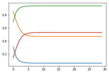
(a) Allocations under tit-for-tat.

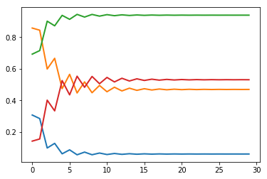
(b) Allocations under the non-lazy proportional dynamic.

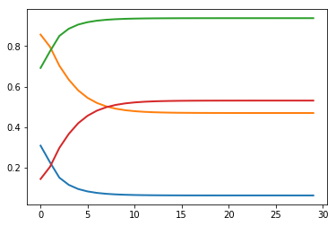
(c) Allocations under the lazy proportional response dynamic with all $\alpha_{i}=1/2$.

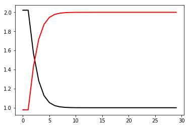
(d) Utilities under tit-for-tat.

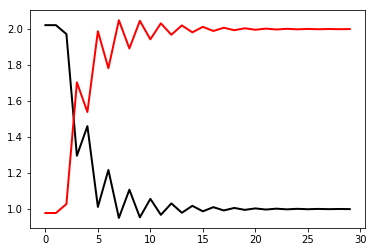
(e) Utilities under the non-lazy proportional dynamic.

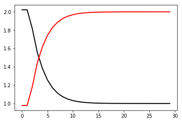
(f) Utilities under the lazy proportional response dynamics with all $\alpha_{i}=1/2$.

Figure 4. Comparison between tit-for-tat, the non-lazy proportional dynamic, and the lazy proportional dynamic, initialized with the same initial fractions of splitting the goods. The valuation matrix is $\mathbf{a}=[[1,2],[1,2]]$ and the initial bids for the proportional response dynamics executions are $\mathbf{b}=[[0.4,0.6],[0.9,0.1]]$. The initial fractions for tit-for-tat are given by $y_{j,i}(0)=b_{i,j}(0)/p_{j}(0)$, where $y_{j,i}(0)$ is the fraction of good $j$ that player $i$ receives in round $0$ for the bids $\mathbf{b}$.

In Figure 4, the $X$ axis shows the round number, while the $Y$ axis shows each utility $u_{i}(t)$ over time and each allocation over time, where an allocation means the fraction received by each player $i$ from good $j$, for each $i,j$, for every time unit $t=0,1,2,\infty$.

In Figure 5, we show a three player economy on which the tit-for-tat dynamic cycles. To obtain the cycling, we consider valuations

$$\textbf{a}=\begin{vmatrix}0&6&4\\ 3&0&9\\ 9&6&0\\ \end{vmatrix}$$

and initial fractions

$$\textbf{y}(0)=\begin{vmatrix}0.0&0.2805339037254016&0.7194660962745985\\ 0.273923422472049&0.0&0.726076577527951\\ 0.491752727261851&0.5082472727381491&0.0\\ \end{vmatrix}$$

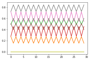
(a) Allocations under tit-for-tat for $T=30$ rounds.

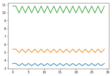
(b) Utilities under tit-for-tat for $T=30$ rounds; same initial conditions as in Figure (a)

Figure 5. Tit-for-tat dynamic cycling for both utilities and allocations with period two. The instance is a three player economy where the matrix does not satisfy the symmetry property under which tit-for-tat is known to converge to market equilibria Wu and Zhang (2007) (Recall this property requires that each good has a common value, i.e. that there exist values $w_{j}$ so that $a_{i,j}=w_{j}$ for each player $i$ and good $j$.).

The fractions oscillate between the values at time $t=0$, equal to $\textbf{y}(0)$, and those from time $t=1$, which are equal to:

$$\textbf{y}(1)=\begin{vmatrix}0.0&0.4552048517736218&0.5447951482263783\\ 0.1553967077250424&0.0&0.8446032922749576\\ 0.5978029457196989&0.402197054280301&0.0\\ \end{vmatrix}$$

We note that market equilibria exist on such graphs and proportional response dynamics converges on these instances for any strictly positive initial bids.

6. Discussion

It would be interesting to see whether a generalization of the dynamic converges for the exchange economy when each player brings multiple goods, as well as to understand more broadly what families of dynamics lead to efficient exchange. It would also be interesting to show a $1/T$ rate of convergence of any last iterate.

7. Acknowledgements

We thank the reviewers for useful feedback that helped improve the paper.

References

- (1)
- Arrow et al. (1959) K. J. Arrow, H. D. Block, and L. Hurwicz. 1959. On the stability of the competitive equilibrium, II. Econometrica: Journal of the Econometric Society (1959), 82–109.
- Ausubel (2004) L. M. Ausubel. 2004. An efficient ascending-bid auction for multiple objects. Am. Econ. Rev 94, 5 (2004), 1452–1475.
- Avigdor-Elgrabli et al. (2014) N. Avigdor-Elgrabli, Y. Rabani, and G. Yadgar. 2014. Convergence of Tâtonnement in Fisher Markets. arXiv preprint arXiv:1401.6637 (2014).
- Babaioff et al. (2017) M. Babaioff, L. Blumrosen, and N. Nisan. 2017. Selling Complementary Goods: Dynamics, Efficiency and Revenue. In ICALP. 134:1–134:14.
- Bei et al. (2019) X. Bei, J. Garg, and M. Hoefer. 2019. Ascending-price algorithms for unknown markets. ACM Trans. Alg. 15, 3 (2019), 37.
- Bhawalkar and Roughgarden (2011) K. Bhawalkar and T. Roughgarden. 2011. Welfare guarantees for combinatorial auctions with item bidding. In SODA. 700–709.
- Birnbaum et al. (2011) B. Birnbaum, N. R. Devanur, and L. Xiao. 2011. Distributed Algorithms via Gradient Descent for Fisher Markets. In Proc. of the 12th ACM Conf. on Electronic Commerce. 127–136.
- Brainard and Scarf (2005) W. C. Brainard and H. E. Scarf. 2005. How to Compute Equilibrium Prices in 1891. The American Journal of Economics and Sociology 64, 1 (2005), 57–83.
- Branzei and Filos-Ratsikas (2019) Simina Branzei and Aris Filos-Ratsikas. 2019. Walrasian Dynamics in Multi-unit Markets. In AAAI.
- Branzei et al. (2018) S. Branzei, R. Mehta, and N. Nisan. 2018. Universal Growth in Production Economies. In Advances in Neural Information Processing Systems 31, S. Bengio, H. Wallach, H. Larochelle, K. Grauman, N. Cesa-Bianchi, and R. Garnett (Eds.). Curran Associates, Inc., 1973–1973.
- Cary et al. (2014) M. Cary, A. Das, B. Edelman, I. Giotis, K. Heimerl, A. R. Karlin, S. D. Kominers, C. Mathieu, and M. Schwarz. 2014. Convergence of Position Auctions Under Myopic Best-Response Dynamics. ACM Trans. Econ. Comput. 2, 3, Article 9 (July 2014), 20 pages. https://doi.org/10.1145/2632226
- Chen and Deng (2011) N. Chen and X. Deng. 2011. On Nash Dynamics of Matching Market Equilibria. (03 2011).
- Chen et al. (2019) P.-A. Chen, C.-J. Lu, and Y.-S. Lu. 2019. An Alternating Algorithm for Finding Linear Arrow-Debreu Market Equilibrium. CoRR abs/1902.01754 (2019). http://arxiv.org/abs/1902.01754
- Chen et al. (2009) X. Chen, D. Dai, Y. Du, and S.-H. Teng. 2009. Settling the complexity of Arrow-Debreu equilibria in markets with additively separable utilities. In Proc. of the 50th Ann. IEEE Symp. on Foundations of Computer Science. 273–282.
- Cheung and Cole (2014) Y. K. Cheung and R. Cole. 2014. Amortized analysis on asynchronous gradient descent. arXiv preprint arXiv:1412.0159 (2014).
- Cheung et al. (2019a) Y. K. Cheung, R. Cole, and N. R. Devanur. 2019a. Tatonnement beyond gross substitutes? Gradient descent to the rescue. Games and Economic Behavior (2019).
- Cheung et al. (2012) Y. K. Cheung, R. Cole, and A. Rastogi. 2012. Tatonnement in ongoing markets of complementary goods. arXiv preprint arXiv:1211.2268 (2012).
- Cheung et al. (2018) Y. K. Cheung, R. Cole, and Y. Tao. 2018. Dynamics of Distributed Updating in Fisher Markets. In Proc. of the 2018 ACM Conf. on Economics and Computation. 351–368.
- Cheung et al. (2019b) Y. K. Cheung, M. Hoefer, and P. Nakhe. 2019b. Tracing Equilibrium in Dynamic Markets via Distributed Adaptation. In Proc. of the 18th Int’l Conf. on Autonomous Agents and MultiAgent Systems. 1225–1233.
- Codenotti et al. (2005a) B. Codenotti, B. McCune, and K. Varadarajan. 2005a. Market equilibrium via the excess demand function. In Proc. of the 37th Ann. ACM Symp. on Theory of Computing. 74–83.
- Codenotti et al. (2005b) B. Codenotti, S. Pemmaraju, and K. Varadarajan. 2005b. On the polynomial time computation of equilibria for certain exchange economies. In Proc. of the 16th Ann. ACM-SIAM Symp. on Discrete Algorithms. 72–81.
- Codenotti et al. (2006) B. Codenotti, A. Saberi, K. Varadarajan, and Y. Ye. 2006. Leontief economies encode nonzero sum two-player games. In Proc. of the 17h Ann. ACM-SIAM Symp. on Discrete Algorithm. 659–667.
- Cole and Fleischer (2008) R. Cole and L. Fleischer. 2008. Fast-converging tatonnement algorithms for one-time and ongoing market problems. In Proc. of the 40th Ann. ACM Symp. on Theory of Computing. 315–324.
- Cornet (1989) B. Cornet. 1989. Linear exchange economies. Cahier Eco-Math, Université de Paris 1 (1989).
- Daskalakis et al. (2015) C. Daskalakis, A. Deckelbaum, and A. Kim. 2015. Near-optimal no-regret algorithms for zero-sum games. GEB 92 (2015), 327–348.
- Daskalakis and Syrgkanis (2016) C. Daskalakis and V. Syrgkanis. 2016. Learning in Auctions: Regret is Hard, Envy is Easy. In FOCS. 219–228.
- Deng et al. (2003) X. Deng, C. Papadimitriou, and S. Safra. 2003. On the complexity of price equilibria. J. Comput. Syst. Sci. 67, 2 (2003), 311–324.
- Devanur et al. (2016) N. R. Devanur, J. Garg, and L. A. Végh. 2016. A rational convex program for linear Arrow-Debreu markets. ACM Trans. on Economics and Computation 5, 1 (2016), 6.
- Devanur and Kannan (2008) N. R. Devanur and R. Kannan. 2008. Market equilibria in polynomial time for fixed number of goods or agents. In Proc. of the 49th Ann. IEEE Symp. on Foundations of Computer Science. 45–53.
- Devanur et al. (2008) N. R. Devanur, C. H. Papadimitriou, A. Saberi, and V. V. Vazirani. 2008. Market equilibrium via a primal–dual algorithm for a convex program. J. ACM 55, 5 (2008), 22.
- Devanur and Vazirani (2003) N. R. Devanur and V. V. Vazirani. 2003. An improved approximation scheme for computing Arrow-Debreu prices for the linear case. In Int’l Conf. on Foundations of Software Technology and Theoretical Computer Science. 149–155.
- Dütting and Kesselheim (2017) P. Dütting and T. Kesselheim. 2017. Best-Response Dynamics in Combinatorial Auctions with Item Bidding. In SODA. 521–533.
- Duan et al. (2016) R. Duan, J. Garg, and K. Mehlhorn. 2016. An improved combinatorial polynomial algorithm for the linear Arrow-Debreu market. In Proc. of the 27th annual ACM-SIAM Symp. on Discrete Algorithms. 90–106.
- Duan and Mehlhorn (2015) R. Duan and K. Mehlhorn. 2015. A combinatorial polynomial algorithm for the linear Arrow-Debreu market. Information and Computation 243 (2015), 112–132.
- Echenique and Wierman (2011) F. Echenique and A. Wierman. 2011. Finding a Walrasian equilibrium is easy for a fixed number of agents. (2011).
- Eisenberg and Gale (1959) E. Eisenberg and D. Gale. 1959. Consensus of subjective probabilities: The pari-mutuel method. The Annals of Mathematical Statistics 30, 1 (1959), 165–168.
- Feldman et al. (2005) M. Feldman, K. Lai, and L. Zhang. 2005. A price-anticipating resource allocation mechanism for distributed shared clusters. In Proc. of the 6th ACM Conf. on Electronic Commerce. 127–136.
- Fisher (1983) F. M. Fisher. 1983. Disequilibrium foundations of equilibrium economics. Cambridge U. Press.
- Fleischer et al. (2008) L. Fleischer, R. Garg, S. Kapoor, R. Khandekar, and A. Saberi. 2008. A Fast and Simple Algorithm for Computing Market Equilibria. In Proc. of the 4th Int’l Workshop on Internet and Network Economics. 19–30.
- Florig (2004) M. Florig. 2004. Equilibrium correspondence of linear exchange economies. Journal of optimization theory and applications 120, 1 (2004), 97–109.
- Freund and Schapire (1999) Y. Freund and R. E Schapire. 1999. Adaptive game playing using multiplicative weights. GEB 29, 1-2 (1999), 79–103.
- Gale (1963) D. Gale. 1963. A note on global instability of competitive equilibrium. Naval Research Logistics Quarterly 10, 1 (1963), 81–87.
- Gale (1976) D. Gale. 1976. The linear exchange model. Journal of Mathematical Economics 3, 2 (1976), 205–209.
- Garg et al. (2015) J. Garg, R. Mehta, M. Sohoni, and V. V. Vazirani. 2015. A complementary pivot algorithm for market equilibrium under separable, piecewise-linear concave utilities. SIAM J. Comp. 44, 6 (2015), 1820–1847.
- Garg and Végh (2019) J. Garg and L. A. Végh. 2019. A strongly polynomial algorithm for linear exchange markets. In Proc. of the 51st Ann. ACM Symp. on Theory of Computing. 54–65.
- Garg and Kapoor (2006) R. Garg and S. Kapoor. 2006. Auction algorithms for market equilibrium. Math. Oper. Res. 31, 4 (2006), 714–729.
- Hassidim et al. (2011) A. Hassidim, H. Kaplan, Y. Mansour, and N. Nisan. 2011. Non-price equilibria in markets of discrete goods. In EC. 295–296.
- Jain (2007) K. Jain. 2007. A Polynomial Time Algorithm for Computing an Arrow-Debreu Market Equilibrium for Linear Utilities. SIAM J. Comput. 37, 1 (April 2007), 303–318.
- Jain et al. (2003) K. Jain, M. Mahdian, and A. Saberi. 2003. Approximating market equilibria. In Approximation, Randomization, and Combinatorial Optimization. Algorithms and Techniques. Springer, 98–108.
- Kelly (1997) F. Kelly. 1997. Charging and rate control for elastic traffic. Europ. Trans. on Telecommunications 8, 1 (1997), 33–37.
- Khalil (2002) H. K. Khalil. 2002. Nonlinear systems. Upper Saddle River (2002).
- Kleinberg et al. (2009) R. Kleinberg, G. Piliouras, and E. Tardos. 2009. Multiplicative updates outperform generic no-regret learning in congestion games. In STOC. 533–542.
- Lucier and Borodin (2010) B. Lucier and A. Borodin. 2010. Price of anarchy for greedy auctions. In SODA. 537–553.
- Lykouris et al. (2016) T. Lykouris, V. Syrgkanis, and E. Tardos. 2016. Learning and Efficiency in Games with Dynamic Population. In SODA. 120–129.
- Mehta et al. (2015) R. Mehta, I. Panageas, and G. Piliouras. 2015. Natural selection as an inhibitor of genetic diversity: Multiplicative weights updates algorithm and a conjecture of haploid genetics [working paper abstract]. In ITCS. 73–73.
- Mertens (2003) J.-F. Mertens. 2003. The limit-price mechanism. Journal of Mathematical Economics 39, 5-6 (2003), 433–528.
- Nisan et al. (2011) N. Nisan, M. Schapira, G. Valiant, and A. Zohar. 2011. Best-response auctions. In EC. 351–360.
- Panageas and Piliouras (2016) I. Panageas and G. Piliouras. 2016. Average case performance of replicator dynamics in potential games via computing regions of attraction. In EC. 703–720.
- Papadimitriou and Piliouras (2016) C. Papadimitriou and G. Piliouras. 2016. From Nash Equilibria to Chain Recurrent Sets: Solution Concepts and Topology. In ITCS. 227–235.
- Roughgarden et al. (2017) T. Roughgarden, V. Syrgkanis, and E. Tardos. 2017. The Price of Anarchy in Auctions. J. Artif. Intell. Res. 59 (2017), 59–101.
- Scarf (1960) H. Scarf. 1960. Some examples of global instability of the competitive equilibrium. International Economic Review 1, 3 (1960), 157–172.
- Scarf (1977) H. Scarf. 1977. The computation of equilibrium prices: an exposition. Technical Report. Cowles Foundation for Research in Economics, Yale University.
- Shapley and Shubik (1977) L. Shapley and M. Shubik. 1977. Trade using one commodity as a means of payment. Journal of Political Economy 85, 5 (1977), 937–968.
- Shmyrev (2009) V. I. Shmyrev. 2009. An algorithm for finding equilibrium in the linear exchange model with fixed budgets. Journal of Applied and Industrial Mathematics 3, 4 (2009), 505.
- Walras (1896) L. Walras. 1896. Éléments d’économie politique pure, ou, Théorie de la richesse sociale. F. Rouge.
- Wu and Zhang (2007) F. Wu and L. Zhang. 2007. Proportional response dynamics leads to market equilibrium. In Proc. of the 39th Ann. ACM Symp. on Theory of Computing. 354–363.
- Ye (2008) Y. Ye. 2008. A path to the Arrow-Debreu competitive market equilibrium. Mathematical Programming 111, 1-2 (2008), 315–348.
- Zhang (2011) L. Zhang. 2011. Proportional response dynamics in the Fisher market. Theoretical Computer Science 412 (2011), 2691–2698.