Optimal location of resources maximizing the total population size in logistic models

Abstract

In this article, we consider a species whose population density solves the steady diffusive logistic equation in a heterogeneous environment modeled with the help of a spatially non constant coefficient standing for a resources distribution. We address the issue of maximizing the total population size with respect to the resources distribution, considering some uniform pointwise bounds as well as prescribing the total amount of resources. By assuming the diffusion rate of the species large enough, we prove that any optimal configuration is bang-bang (in other words an extreme point of the admissible set) meaning that this problem can be recast as a shape optimization problem, the unknown domain standing for the resources location. In the one-dimensional case, this problem is deeply analyzed, and for large diffusion rates, all optimal configurations are exhibited. This study is completed by several numerical simulations in the one dimensional case.

Keywords: diffusive logistic equation, rearrangement inequalities, symmetrization, optimal control, shape optimization, optimality conditions.

AMS classification: 49K20, 35Q92, 49J30, 34B15.

1 Introduction

1.1 Motivations and state of the art

In this article, we investigate an optimal control problem arising in population dynamics. Let us consider the population density ${\theta_{m,\mu}}$ of a given species evolving in a bounded and connected domain ${\Omega}$ in $\textrm{I\kern-2.10007ptR}^{n}$ with $n\in\textrm{I\kern-2.10007ptN}^{*}$, having a $\mathscr{C}^{2}$ boundary. In what follows, we will assume that ${\theta_{m,\mu}}$ is the positive solution of the steady logistic-diffusive equation (denoted (LDE) in the sequel) which writes

$$\left\{\begin{array}[]{ll}\mu{\Delta}{\theta_{m,\mu}}(x)+(m(x)-{\theta_{m,\mu}}(x)){\theta_{m,\mu}}(x)=0&x\in{\Omega},\\ \frac{\partial{\theta_{m,\mu}}}{\partial\nu}=0&x\in\partial{\Omega},\end{array}\right.$$ (LDE)

where $m\in L^{\infty}({\Omega})$ stands for the resources distribution and $\mu>0$ stands for the dispersal ability of the species, also called diffusion rate. From a biological point of view, the real number $m(x)$ is the local intrinsic growth rate of species at location $x$ of the habitat ${\Omega}$ and can be seen as a measure of the resources available at $x$.

As will be explained below, we will only consider non-negative resource distributions.$m$, i.e such that $m\in L^{\infty}_{+}({\Omega})=\left\{m\in L^{\infty}({\Omega})\,,m\geqslant 0\text{ a.e}\right\}$. In view of investigating the influence of spatial heterogeneity on the model, we consider the optimal control problem of maximizing the functional

$${\mathcal{F}_{\mu}}:L_{+}^{\infty}({\Omega})\ni m\mapsto\fint_{\Omega}{\theta_{m,\mu}},$$

where the notation $\fint$ denotes the average operator, in other words $\fint_{\Omega}f=\frac{1}{|{\Omega}|}\int_{\Omega}f$. The functional $F$ stands for the total population size, in order to further our understanding of spatial heterogeneity on population dynamics.
In the framework of population dynamics, the density $\theta_{m,\mu}$ solving Equation (LDE) can be interpreted as a steady state associated to the following evolution equation

$$\left\{\begin{array}[]{ll}\frac{\partial u}{\partial t}(t,x)=\mu{\Delta}u(t,x)+u(t,x)(m(x)-u(t,x))&t>0,\ x\in{\Omega}\\ \frac{\partial u}{\partial\nu}(t,x)=0&t>0,\ x\in\partial{\Omega}\\ u(0,x)=u^{0}(x)\geqslant 0\,,u^{0}\neq 0&x\in{\Omega}\\ \end{array}\right.$$ (LDEE)

modeling the spatiotemporal behavior of a population density $u$ in a domain $\Omega$ with the spatially heterogeneous resource term $m$.

The pioneering works by Fisher [12], Kolmogorov-Petrovski-Piskounov [27] and Skellam [40] on the logistic diffusive equation were mainly concerned with the spatially homogeneous case. Thereafter, many authors investigated the influence of spatial heterogeneity on population dynamics and species survival. In [23], propagation properties in a patch model environment are studied. In [22], a spectral condition for species survival in heterogeneous environments has been derived, while [26] deals with the influence of fragmentation and concentration of resources on population dynamics. These works were followed by [2] dedicated to an optimal design problem, that will be commented in the sequel.

Investigating existence and uniqueness properties of solutions for the two previous equations as well as their regularity properties boils down to the study of spectral properties for the linearized operator

$$\mathcal{L}:\mathcal{D}(\mathcal{L})\ni f\mapsto\mu\Delta f+mf,$$

where the domain of $\mathcal{L}$ is $\mathcal{D}(\mathcal{L})=\{f\in L^{2}({\Omega})\mid\Delta f\in L^{2}({\Omega})\}$ and of its first eigenvalue $\lambda_{1}(m,\mu)$, characterized by the Courant-Fischer formula

$$\lambda_{1}(m,\mu):=\underset{f\in W^{1,2}(\Omega),\int_{\Omega}f^{2}=1}{\sup}\left\{-\mu\int_{\Omega}|\nabla f|^{2}+\int_{\Omega}mf^{2}\right\}.$$ (1)

Indeed, the positiveness of $\lambda(m,\mu)$ is a sufficient condition ensuring the well-posedness of equations (LDEE) and (LDE) ([2]). Then, Equation (LDE) has a unique positive solution ${\theta_{m,\mu}}\in W^{1,2}({\Omega})$. Furthermore, for any $p\geqslant 1$, ${\theta_{m,\mu}}$ belongs to $W^{2,p}({\Omega})$, and there holds

$$0<\underset{\overline{\Omega}}{\inf}\,{\theta_{m,\mu}}\leqslant{\theta_{m,\mu}}\leqslant\|m\|_{L^{\infty}({\Omega})}.$$ (2)

Moreover, the steady state ${\theta_{m,\mu}}$ is globally asymptotically stable: for any $u_{0}\in W^{1,2}({\Omega})$ such that $u_{0}\geqslant 0$ a.e. in ${\Omega}$ and $u_{0}\neq 0$ , one has

$$\|u(t,\cdot)-{\theta_{m,\mu}}\|_{L^{\infty}({\Omega})}\underset{t\rightarrow+\infty}{\longrightarrow}0.$$

where $u$ denotes the unique solution of (LDEE) with initial state $u_{0}$ (belonging to $L^{2}(0,T;W^{1,2}({\Omega}))$ for every $T>0$).

The importance of $\lambda_{1}(m,\mu)$ for stability issues related to population dynamics models was first noted in simple cases by Ludwig, Aronson and Weinberger [34]. Let us mention [10] where the case of diffusive Lotka-Volterra equations is investigated.

To guarantee that $\lambda_{1}(m,\mu)>0$, it is enough to work with distributions of resources $m$ satisfying the assumption

$$m\in L^{\infty}_{+}({\Omega})\quad\text{where}\quad L^{\infty}_{+}({\Omega})=\left\{m\in L^{\infty}({\Omega}),\ \ \int_{\Omega}m>0\right\}.$$ (H1)

Note that the issue of maximizing this principal eigenvalue was addressed for instance in [19, 20, 28, 33, 39].

In the survey article [32], Lou suggests the following problem: the parameter $\mu>0$ being fixed, which weight $m$ maximizes the total population size among all uniformly bounded elements of $L^{\infty}({\Omega})$?

In this article, we aim at providing partial answers to this issue, and more generally new results about the influence of the spatial heterogeneity $m(\cdot)$ on the total population size.

For that purpose, let us introduce the total population size functional, defined for a given $\mu>0$ by

$${\mathcal{F}_{\mu}}:L^{\infty}_{+}({\Omega})\ni m\longmapsto\fint_{\Omega}{\theta_{m,\mu}},$$ (3)

where ${\theta_{m,\mu}}$ denotes the solution of equation (LDE).

Let us mention several previous works dealing with the maximization of the total population size functional. It is shown in [31] that, among all weights $m$ such that $\fint_{\Omega}m=m_{0}$, there holds ${\mathcal{F}_{\mu}}(m)\geqslant{\mathcal{F}_{\mu}}(m_{0})=m_{0}$; this inequality is strict whenever $m$ is nonconstant. Moreover, it is also shown that the problem of maximizing ${\mathcal{F}_{\mu}}$ over $L^{\infty}_{+}({\Omega})$ has no solution.

Remark 1.

The fact that $m\equiv m_{0}$ is a minimum for ${\mathcal{F}_{\mu}}$ among the resources distributions $m$ satisfying $\fint_{\Omega}m=m_{0}$ relies on the following observation: multiplying (LDE) by $\frac{1}{{\theta_{m,\mu}}}$ and integrating by parts yields

$$\mu\fint_{\Omega}\frac{|{\nabla}{\theta_{m,\mu}}|^{2}}{{\theta_{m,\mu}}^{2}}+\fint_{\Omega}(m-{\theta_{m,\mu}})=0.$$ (4)

and therefore, ${\mathcal{F}_{\mu}}(m)=m_{0}+\mu\int_{\Omega}\frac{|{\nabla}{\theta_{m,\mu}}|^{2}}{{\theta_{m,\mu}}^{2}}\geqslant m_{0}={\mathcal{F}_{\mu}}(m_{0})$ for all $m\in L^{\infty}_{+}({\Omega})$ such that $\fint_{\Omega}m=m_{0}$. It follows that the constant function equal to $m_{0}$ is a global minimizer of ${\mathcal{F}_{\mu}}$ over $\{m\in L^{\infty}_{+}({\Omega})\,,\fint_{\Omega}m=m_{0}\}.$

In the recent article [1], it is shown that, when ${\Omega}=(0,\ell)$, one has

$$\forall\mu>0,\ \forall m\in L_{+}^{\infty}({\Omega})\mid m\geqslant 0\text{ a.e.},\qquad\fint_{\Omega}{\theta_{m,\mu}}\leqslant 3\fint_{\Omega}m.$$

This inequality is sharp, although the right-hand side is never reached, and the authors exhibit a sequence $(m_{k},\mu_{k})_{k\in\textrm{I\kern-1.47005ptN}}$ such that $\fint_{\Omega}\theta_{m_{k},\mu_{k}}/\fint_{\Omega}m_{k}\rightarrow 3$ as $k\to+\infty$, but for such a sequence there holds $\|m_{k}\|_{L^{\infty}({\Omega})}\rightarrow+\infty$ and $\mu_{k}\rightarrow 0$ as $k\to+\infty$.
In [32], it is proved that, without $L^{1}$ or $L^{\infty}$ bounds on the weight function $m$, the maximization problem is ill-posed. It is thus natural to introduce two parameters $\kappa,m_{0}>0$, and to restrict our investigation to the class

$$\mathcal{M}_{m_{0},\kappa}({\Omega}):=\left\{m\in L^{\infty}({\Omega})\,,0\leqslant m\leqslant\kappa\text{ a.e }\,,\fint_{\Omega}m=m_{0}\right\}.$$ (5)

It is notable that in [9], the more general functional $J_{B}$ defined by

$$J_{B}(m)=\int_{\Omega}(\theta_{m,\mu}-Bm^{2})\qquad\hbox{ for }B\geqslant 0$$

is introduced. In the case $B=0$, the authors apply the so-called Pontryagin principle, show the Gâteaux-differentiability of $J_{B}$ and carry out numerical simulations backing up the conjecture that maximizers of $J_{0}$ over $\mathcal{M}_{m_{0},\kappa}({\Omega})$ are of bang-bang type.

However, proving this bang-bang property is a challenge. The analysis of optimal conditions is quite complex, because the sensitivity of the functional ”total population size” with respect to $m(\cdot)$ is directly related to the solution of an adjoint state, solving a linearized version of (LDE). Deriving and exploiting the properties of optimal configurations therefore requires a thorough understanding of the $\theta_{m,\mu}$ behavior as well as the associated state. To do this, we are introducing a new asymptotic method to exploit optimal conditions.

We will investigate two properties of the maximizers of the total population size function ${\mathcal{F}_{\mu}}$.

1. Pointwise constraints. The main issue that will be addressed in what follows is the bang-bang character of optimal weights $m^{*}(\cdot)$, in other words, whether $m^{*}$ is equal to 0 or $\kappa$ almost everywhere. Noting that $\mathcal{M}_{m_{0},\kappa}({\Omega})$ is a convex set and that bang-bang functions are the extreme points of this convex set, this question rewrites:

   Are the maximizers $m^{*}$ extreme points of the set $\mathcal{M}_{m_{0},\kappa}({\Omega})$?

   In our main result (Theorem 1) we provide a positive answer for large diffusivities. It is notable that our proof rests upon a well-adapted expansion of the solution ${\theta_{m,\mu}}$ of (LDE) with respect to the diffusivity $\mu$.

   This approach could be considered unusual, since such results are usually obtained by an analysis of the properties of the adjoint state (or switching function). However, since the switching function very implicitly depends on the design variable $m(\cdot)$, we did not obtain this result in this way.

2. Concentration-fragmentation. It is well known that resource concentration (which means that the distribution of resources $m$ decreases in all directions, see Definition 2 for a specific statement) promotes the survival of species [2]. On the contrary, we will say that a resource distribution $m=\kappa\chi_{E}$, where $E$ is a subset of ${\Omega}$, is fragmented when the $E$ set is disconnected. In the figure 1, ${\Omega}$ is a square, and the intuitive notion of concentration-fragmentation of resource distribution is illustrated.

   

   

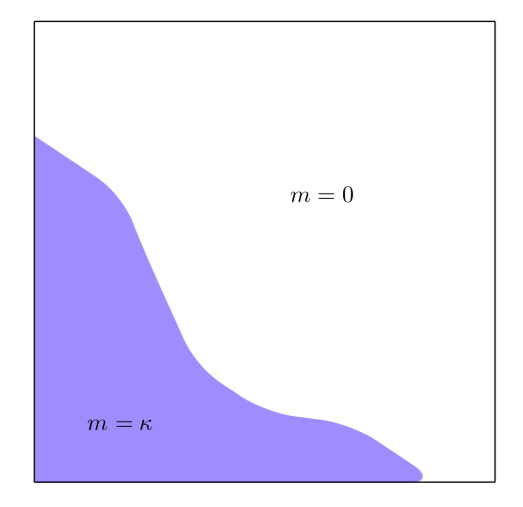
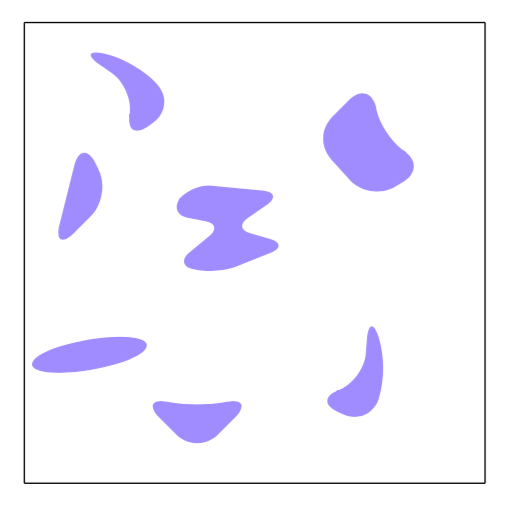
   Figure 1: ${\Omega}=(0,1)^{2}$. The left distribution is ”concentrated” (connected) whereas the right one is fragmented (disconnected).

   A natural issue related to qualitative properties of maximizers is thus

   Are maximizers $m^{*}$ concentrated? Fragmentated?

   In Theorem 2, we consider the case of a orthotope shape habitat, and we show that concentration occurs for large diffusivities: if $m_{\mu}$ maximizes ${\mathcal{F}_{\mu}}$ over $\mathcal{M}_{m_{0},\kappa}({\Omega})$, the sequence $\{m_{\mu}\}_{\mu>0}$ strongly converges in $L^{1}({\Omega})$ to a concentrated distribution as $\mu\to\infty$,.
   In the one-dimensional case, we also prove that if the diffusivity is large enough, there are only two maximizers, that are plotted on Fig. 2 (see Theorem 3).

   

   

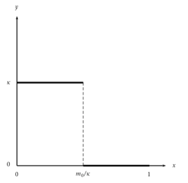
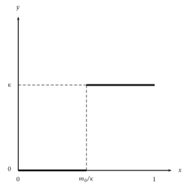
   Figure 2: ${\Omega}=(0,1)$. Plot of the only two maximizers of ${\mathcal{F}_{\mu}}$ over $\mathcal{M}_{m_{0},\kappa}({\Omega})$.

   Finally, in the one-dimensional case, we obtain a surprising result: fragmentation may be better than concentration for small diffusivities (see Theorem 4 and Fig. 3 below).

   

   

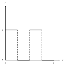
   Figure 3: ${\Omega}=(0,1)$. A double crenel (on the left) is better than a single one (on the right).

   This is surprising because in many problems of optimizing the logistic-diffusive equation, it is expected that the best disposition of resources will be concentrated.

1.2 Main results

In the whole article, the notation $\chi_{I}$ will be used to denote the characteristic function of a measurable subset $I$ of $\textrm{I\kern-2.10007ptR}^{n}$, in other words, the function equal to 1 in $I$ and 0 elsewhere.

For the reasons mentioned in Section 1.1, it is biologically relevant to consider the class of admissible weights $\mathcal{M}_{m_{0},\kappa}({\Omega})$ defined by (5), where $\kappa>0$ and $m_{0}>0$ denote two positive parameters such that $m_{0}<\kappa$ (so that this set is nontrivial).

We will henceforth consider the following optimal design problem.

Optimal design problem. Fix $n\in\textrm{I\kern-2.10007ptN}^{*}$, $\mu>0$, $\kappa>0$, $m_{0}\in(0,\kappa)$ and let ${\Omega}$ be a bounded connected domain of $\textrm{I\kern-2.10007ptR}^{n}$ having a $\mathscr{C}^{2}$ boundary. We consider the optimization problem $$\sup_{m\in\mathcal{M}_{\kappa,m_{0}}({\Omega})}{\mathcal{F}_{\mu}}(m).$$ ($\mathcal{P}_{\mu}^{n}$)

As will be highlighted in the sequel, the existence of a maximizer follows from a direct argument. We will thus investigate the qualitative properties of maximizers described in the previous section (bang-bang character, concentration/fragmentation phenomena).

For the sake of readability, almost all the proofs are postponed to Section 2.

Let us stress that the bang-bang character of maximizer is of practical interest in view of spreading resources in an optimal way. Indeed, in the case where a maximizer $m^{*}$ writes $m^{*}=\kappa\chi_{E}$, the total size of population is maximized by locating all the resources on $E$.

1.2.1 First property

We start with a preliminary result related to the saturation of pointwise constraints for Problem ($\mathcal{P}_{\mu}^{n}$), valid for all diffusivities $\mu$. It is obtained by exploiting the first order optimality conditions for Problem ($\mathcal{P}_{\mu}^{n}$), written in terms of an adjoint state.

Proposition 1.

Let $n\in\textrm{I\kern-2.10007ptN}^{*}$, $\mu>0$, $\kappa>0$, $m_{0}\in(0,\kappa)$. Let $m^{*}$ be a solution of Problem ($\mathcal{P}_{\mu}^{n}$). Then, the set $\{m=\kappa\}\cup\{m=0\}$ has a positive measure

1.2.2 The bang-bang property holds for large diffusivities

For large values of $\mu$, we will prove that the variational problem can be recast in terms of a shape optimization problem, as underlined in the next results.

Theorem 1.

Let $n\in\textrm{I\kern-2.10007ptN}^{*}$, $\kappa>0$, $m_{0}\in(0,\kappa)$. There exists a positive number $\mu^{*}=\mu^{*}({\Omega},\kappa,m_{0})$ such that, for every $\mu\geqslant\mu^{*}$, the functional ${\mathcal{F}_{\mu}}$ is strictly convex. As a consequence, for $\mu\geqslant\mu^{*}$, any maximizer of ${\mathcal{F}_{\mu}}$ over $\mathcal{M}_{m_{0},\kappa}({\Omega})$ (or similarly any solution of Problem ($\mathcal{P}_{\mu}^{n}$)) is moreover of bang-bang type.

We emphasize that the proof of Theorem 1 is quite original, since it does not rest upon the exploitation of adjoint state properties, but upon the use of a power series expansions in the diffusivity $\mu$ of the solution ${\theta_{m,\mu}}$ of (LDE), as well as their derivative with respect to the design variable m. In particular, this expansion is used to prove that, if $\mu$ is large enough, then the function ${\mathcal{F}_{\mu}}$ is strictly convex. Since the extreme points of $\mathcal{M}_{m_{0},\kappa}({\Omega})$ are bang-bang resources functions, the conclusion readily follows.
This theorem justifies that Problem ($\mathcal{P}_{\mu}^{n}$) can be recast as a shape optimization problem. Indeed, every maximizer $m^{*}$ is of the form $m^{*}=\kappa\chi_{E}$ where $E$ is a measurable subset such that $|E|=m_{0}|{\Omega}|/\kappa$.

Remark 2.

We can rewrite this result in terms of shape optimization, by considering as main unknown the subset $E$ of ${\Omega}$ where resources are located: indeed, under the assumptions of Theorem 1, there exists a positive number $\mu^{*}=\mu^{*}({\Omega},\kappa,m_{0})$ such that, for every $\mu\geqslant\mu^{*}$, the shape optimization problem

$$\sup_{E\subset{\Omega},\ |E|=m_{0}|{\Omega}|/\kappa}{\mathcal{F}_{\mu}}(\kappa\chi_{E}),$$ (6)

where the supremum is taken over all measurable subset $E\subset{\Omega}$ such that $|E|=m_{0}|{\Omega}|/\kappa$, has a solution. We underline the fact that, for such a shape functional, which is “non-energetic” in the sense that the solution of the PDE involved cannot be seen as a minimizer of the same functional, proving the existence of maximizers is usually intricate.

1.2.3 Concentration occurs for large diffusivities

In this section, we state two results suggesting concentration properties for the solutions of Problem ($\mathcal{P}_{\mu}^{n}$) may hold for large diffusivities.
For that purpose, let us introduce the function space

$$X:=W^{1,2}({\Omega})\cap\left\{u\in W^{1,2}({\Omega})\,,\fint_{\Omega}u=0\right\}$$ (7)

and the energy functional

$$\mathcal{E}_{m}:X\ni u\mapsto\frac{1}{2}\fint_{\Omega}|{\nabla}u|^{2}-m_{0}\fint_{\Omega}mu.$$ (8)

Theorem 2.

[$\Gamma$-convergence property]

1. Let ${\Omega}$ be a domain with a $\mathscr{C}^{2}$ boundary. For any $\mu>0$, let $m_{\mu}$ be a solution of Problem ($\mathcal{P}_{\mu}^{n}$). Any $L^{1}$ closure point of $\{m_{\mu}\}_{\mu>0}$ as $\mu\to\infty$ is a solution of the optimal design problem

   $$\min_{m\in\mathcal{M}_{m_{0},\kappa}({\Omega})}\min_{u\in X}\mathcal{E}_{m}(u).$$ (9)

2. In the case of a two dimensional orthotope ${\Omega}=(0;a_{1})\times(0;a_{2})$, any solution of the asymptotic optimization problem (9) decreases in every direction.

As will be clear in the proof, this theorem is a $\Gamma$-convergence property.

In the one-dimensional case, one can refine this result by showing that, for $\mu$ large enough, the maximizer is a step function.

Theorem 3.

Let us assume that $n=1$ and ${\Omega}=(0,1)$. Let $\kappa>0$, $m_{0}\in(0,\kappa)$. There exists $\hat{\mu}>0$ such that, for any $\mu\geqslant\hat{\mu}$, any solution $m$ of Problem ($\mathcal{P}_{\mu}^{n}$) is equal a.e. to either $\tilde{m}$ or $\tilde{m}(1-\cdot)$, where $\tilde{m}=\kappa\chi_{(1-\ell,1)}$ and $\ell=m_{0}/\kappa$.

1.2.4 Fragmentation may occur for small diffusivities

Let us conclude by underlining that the statement of Theorem 3 cannot be true for all $\mu>0$. Indeed, we provide an example in Section 3.1 where a double-crenel growth rate gives a larger total population size than the simple crenel $\tilde{m}$ of Theorem 3.

Theorem 4.

The function $\tilde{m}=\kappa\chi_{(1-\ell,1)}$ (and $\tilde{m}(1-\cdot)=\kappa\chi_{(0,\ell)}$) does not solve Problem ($\mathcal{P}_{\mu}^{n}$) for small values of $\mu$. More precisely, if we extend $\tilde{m}$ outside of $(0,1)$ by periodicity, there exists $\mu>0$ such that

$${\mathcal{F}_{\mu}}\big{(}\tilde{m}(2~{}\cdot)\big{)}>{\mathcal{F}_{\mu}}(\tilde{m}).$$

This result is quite unusual. For the optimization of the first eigenvalue $\lambda_{1}(m,\mu)$ defined by (1) with respect to $m$ on the interval $(0;1)$

$$\sup_{m\in\mathcal{M}((0;1))}\lambda_{1}(m,\mu)$$

we know (see [2]) that the only solutions are $\tilde{m}$ and $\tilde{m}(1-\cdot)$, for any $\mu$.

It is notable that the following result is a byproduct of Theorem 4 above.

Corollary 1.

There exists $\mu>0$ such that the problems

$$\sup_{m\in\mathcal{M}((0;1))}\lambda_{1}(m,\mu)$$

and

$$\sup_{m\in\mathcal{M}((0;1))}{\mathcal{F}_{\mu}}(m)$$

do not have the same maximizers.

For further comments on the relationship between the main eigenvalue and the total size of the population, we refer to [35], where an asymptotic analysis of the main eigenvalue (relative to $\mu$ as $\mu\to+\infty$) is performed, and the references therein.

We conclude this section by mentioning the recent work [36], that was reported to us when we wrote this article. They show that, if we assume the optimal distribution of regular resources (more precisely, Riemann integrable), then it is necessarily of bang-bang type. Their proof is based on a perturbation argument valid for all $\mu>$0. However, proving such regularity is generally quite difficult. Our proof, although it is not valid for all $\mu$, is not based on such a regularity assumption, but these two combined results seem to suggest that all maximizers of this problem are of bang-bang type.

1.3 Tools and notations

In this section, we gather some useful tools we will use to prove the main results.

Rearrangements of functions and principal eigenvalue.

Let us first recall several monotonicity and regularity related to the principal eigenvalue of the operator $\mathcal{L}$.

Proposition 2.

[10] Let $m\in L^{\infty}_{+}({\Omega})$ and $\mu>0$.

• The mapping $\textrm{I\kern-2.10007ptR}_{+}^{*}\ni\mu\mapsto\lambda_{1}(m,\mu)$ is continuous and non-increasing.

• If $m\leqslant m_{1}$, then $\lambda_{1}(m,\mu)\leqslant\lambda_{1}(m_{1},\mu)$, and the equality is true if, and only if $m=m_{1}$ a.e. in ${\Omega}$.

In the proof of Theorem 3, we will use rearrangement inequalities at length. Let us briefly recall the notion of decreasing rearrangement.

Definition 1.

For a given function $b\in L^{2}(0,1)$, one defines its monotone decreasing (resp. monotone increasing) rearrangement $b_{dr}$ (resp. $b_{br}$) on $(0,1)$ by $b_{dr}(x)=\sup\{c\in\textrm{I\kern-2.10007ptR}\mid x\in\Omega_{c}^{*}\}$, where $\Omega_{c}^{*}=(1-|\Omega_{c}|,1)$ with $\Omega_{c}=\{b>c\}$ (resp. $b_{br}(\cdot)=b_{dr}(1-\cdot)$).

The functions $b_{dr}$ and $b_{br}$ enjoy nice properties. In particular, the Polyà-Szego and Hardy-Littlewood inequalities allow to compare integral quantities depending on $b$, $b_{dr}$, $b_{br}$ and their derivative.

Theorem ([24, 29]).

Let $u$ be a non-negative and measurable function.

• If $\psi$ is any measurable function from $\textrm{I\kern-2.10007ptR}_{+}$ to IR, then

  $$\int_{0}^{1}\psi(u)=\int_{0}^{1}\psi(u_{dr})=\int_{0}^{1}\psi(u_{br})\quad\text{(equimeasurability)};$$

• If $u$ belongs to $W^{1,p}(0,1)$ with $1\leqslant p$, then

  $$\int_{0}^{1}(u^{\prime})^{p}\geqslant\int_{0}^{1}(u_{br}^{\prime})^{p}=\int_{0}^{1}(u_{dr}^{\prime})^{p}\quad\text{(P\'{o}lya inequality)};$$

• If $u$, $v$ belong to $L^{2}(0,1)$, then

  $$\int_{0}^{1}uv\leqslant\int_{0}^{1}u_{br}v_{br}=\int_{0}^{1}u_{dr}v_{dr}\quad\text{(Hardy-Littlewood inequality)};$$

The equality case in the Polyà-Szego inequality is the object of the Brothers-Ziemer theorem (see e.g. [11]).

Symmetric decreasing functions

In higher dimensions, in order to highlight concentration phenomena, we will use another notion of symmetry, namely monotone symmetric rearrangements that are extensions of monotone rearrangements in one dimension. Here, ${\Omega}$ denotes the $n$-dimensional orthotope $\prod_{i=1}^{n}(a_{i},b_{i})$.

Definition 2.

For a given function $b\in L^{1}({\Omega})$, one defines its symmetric decreasing rearrangement $b_{sd}$ on ${\Omega}$ as follows: first fix the $n-1$ variables $x_{2},\dots,x_{n}$. Define $b_{1,sd}$ as the monotone decreasing rearrangement of $x\mapsto b(x,x_{2},\dots,x_{n})$. Then fix $x_{1},x_{3},\dots,x_{n}$ and define $b_{2,sd}$ as the monotone decreasing rearrangement of $x\mapsto b_{1,sd}(x_{1},x,\dots,x_{n})$. Perform such monotone decreasing rearrangements successively. The resulting function is the symmetric decreasing rearrangement of $b$.
We define the symmetric increasing rearrangement in a direction $i$ a similar fashion and write it $b_{i,id}$. Note that, in higher dimensions, the definition of decreasing rearrangement strongly depends on the order in which the variables are taken.

Similarly to the one-dimensional case, the Pólya-Szego and Hardy-Littlewood inequalities allow us to compare integral quantities.

Theorem ([2, 3]).

Let $u$ be a non-negative and measurable function defined on a box ${\Omega}=\prod_{i=1}^{n}(0;a_{i})$.

• If $\psi$ is any measurable function from $\textrm{I\kern-2.10007ptR}_{+}$ to IR, then

  $$\int_{\Omega}\psi(u)=\int_{\Omega}\psi(u_{sd})=\int_{\Omega}\psi(u_{sd})\quad\text{(equimeasurability)};$$

• If $u$ belongs to $W^{1,p}({\Omega})$ with $1\leqslant p$, then, for every $i\in\textrm{I\kern-2.10007ptN}_{N}$, $[a_{i};b_{i}]=\omega_{1,i}\cup\omega_{2,i}\cup\omega_{3,i}$, where the map $(x_{1},\dots,x_{i-1},x_{i+1},\dots,x_{N})\mapsto u(x_{1},\dots,x_{n})$ is decreasing if $x_{i}\in\omega_{1,i}$, increasing if $x_{i}\in\omega_{2,i}$ and constant if $x_{i}\in\omega_{3,i}$.

  $$\int_{\Omega}|{\nabla}u|^{p}\geqslant\int_{\Omega}|{\nabla}u_{sd}|^{p}\quad\text{(P\'{o}lya inequality)};$$

  Furthermore, if, for any $i\in\textrm{I\kern-2.10007ptN}_{n}$, $\int_{\Omega}|{\nabla}u|^{p}=\int_{\Omega}|{\nabla}u_{i,sd}|^{p}$ then there exist three measurable subets $\omega_{i,1}\,,\omega_{i,2}$ and $\omega_{i,3}$ of $(0;a_{i})$ such that

  1. $(0;a_{i})=\omega_{i,1}\cup\omega_{i,2}\omega_{i,3}$,

  2. $u=u_{i,bd}$ on $\prod_{k=1}^{i-1}(0;a_{k})\times\omega_{i,1}\times\prod_{k=i+1}^{n}(0;a_{k})$,

  3. $u=u_{i,id}$ on $\prod_{k=1}^{i-1}(0;a_{k})\times\omega_{i,2}\times\prod_{k=i+1}^{n}(0;a_{k})$,

  4. $u=u_{i,bd}=u_{i,id}$ on $\prod_{k=1}^{i-1}(0;a_{k})\times\omega_{i,3}\times\prod_{k=i+1}^{n}(0;a_{k})$.

• If $u$, $v$ belong to $L^{2}({\Omega})$, then

  $$\int_{\Omega}uv\leqslant\int_{\Omega}u_{sd}v_{sd}\quad\text{(Hardy-Littlewood inequality)};$$

Poincaré constants and elliptic regularity results.

We will denote by $c_{\ell}^{(p)}$ the optimal positive constant such that for every $p\in[1,+\infty)$, $f\in L^{p}({\Omega})$ and $u\in W^{1,p}({\Omega})$ satisfying

$$\Delta u=f\quad\text{in }\mathcal{D}^{\prime}({\Omega}),$$

there holds

$$\|u\|_{W^{2,p}({\Omega})}\leqslant c_{\ell}^{(p)}\left(\|f\|_{L^{p}({\Omega})}+\|u\|_{L^{p}({\Omega})}\right).$$

The optimal constant in the Poincaré-Wirtinger inequality will be denoted by $C_{PW}^{(p)}({\Omega})$. This inequality reads: for every $u\in W^{1,p}({\Omega})$,

$$\bigg{\|}u-\fint_{\Omega}u\bigg{\|}_{L^{p}({\Omega})}\leqslant C_{PW}^{(p)}({\Omega})\|{\nabla}u\|_{L^{p}({\Omega})}.$$ (10)

We will also use the following regularity results:

Theorem.

([41, Theorem 9.1]) Let ${\Omega}$ be a $\mathscr{C}^{2}$ domain. There exists a constant $C_{\Omega}>0$ such that, if $f\in L^{\infty}({\Omega})$ and $u\in W^{1,2}({\Omega})$ solve

$$\left\{\begin{array}[]{ll}-\Delta u=f&\text{ in }{\Omega},\\ \frac{\partial u}{\partial\nu}=0&\text{ on }\partial{\Omega},\end{array}\right.$$ (11)

then

$$\|{\nabla}u\|_{L^{1}({\Omega})}\leqslant C_{\Omega}\|f\|_{L^{1}({\Omega})}.$$ (12)

Theorem.

([8, Theorem 1.1]) Let ${\Omega}$ be a $\mathscr{C}^{2}$ domain. There exists a constant $C_{\Omega}>0$ such that, if $f\in L^{\infty}({\Omega})$ and $u\in W^{1,2}({\Omega})$ solve

$$\left\{\begin{array}[]{ll}-\Delta u=f&\text{ in }{\Omega},\\ \frac{\partial u}{\partial\nu}=0&\text{ on }\partial{\Omega},\end{array}\right.$$ (13)

then

$$\|{\nabla}u\|_{L^{\infty}({\Omega})}\leqslant C_{\Omega}\|f\|_{L^{\infty}({\Omega})}.$$ (14)

Remark 1.

This result is in fact a corollary [8, Theorem 1.1]. In this article it is proved that the $L^{\infty}$ norm of the gradient of $f$ is bounded by the Lorentz norm $L^{n,1}({\Omega})$ of $f$, which is automatically controlled by the $L^{\infty}({\Omega})$ norm of $f$.

Note that Stampacchia’s orginal result deals with Dirichlet boundary conditions. However, the same duality arguments provide the result for Neumann boundary conditions.

Theorem.

([30]) Let $r\in(1;+\infty)$. There exists $C_{r}>0$ such that, if $f\in L^{r}({\Omega})$ and if $u\in W^{1,r}({\Omega})$ be a solution of

$$\left\{\begin{array}[]{ll}-\Delta u=\operatorname{div}(f)&\text{ in }{\Omega},\\ \frac{\partial u}{\partial\nu}=0&\text{ on }\partial{\Omega},\end{array}\right.$$ (15)

then there holds

$$\|{\nabla}u\|_{L^{r}({\Omega})}\leqslant C_{r}\|f\|_{L^{r}({\Omega})}.$$ (16)

2 Proofs of the main results

2.1 First order optimality conditions for Problem ($\mathcal{P}_{\mu}^{n}$)

To prove the main results, we first need to state the first order optimality conditions for Problem ($\mathcal{P}_{\mu}^{n}$). For that purpose, let us introduce the tangent cone to $\mathcal{M}_{m_{0},\kappa}({\Omega})$ at any point of this set.

Definition 3.

([15, chapter 7]) For every $m\in\mathcal{M}_{m_{0},\kappa}({\Omega})$, the tangent cone to the set $\mathcal{M}_{m_{0},\kappa}({\Omega})$ at $m$, denoted by $\mathcal{T}_{m,\mathcal{M}_{m_{0},\kappa}({\Omega})}$ is the set of functions $h\in\mathrm{L}^{\infty}({\Omega})$ such that, for any sequence of positive real numbers $\varepsilon_{n}$ decreasing to $0$, there exists a sequence of functions $h_{n}\in\mathrm{L}^{\infty}({\Omega})$ converging to $h$ as $n\rightarrow+\infty$, and $m+\varepsilon_{n}h_{n}\in\mathcal{M}_{m_{0},\kappa}({\Omega})$ for every $n\in\textrm{I\kern-2.10007ptN}$.

We will show that, for any $m\in\mathcal{M}_{m_{0},\kappa}({\Omega})$ and any admissible perturbation $h\in\mathcal{T}_{m,\mathcal{M}_{m_{0},\kappa}({\Omega})}$, the functional ${\mathcal{F}_{\mu}}$ is twice Gâteaux-differentiable at $m$ in direction $h$. To do that, we will show that the solution mapping

$$\mathcal{S}:m\in\mathcal{M}_{m_{0},\kappa}({\Omega})\mapsto{\theta_{m,\mu}}\in L^{2}({\Omega}),$$

where ${\theta_{m,\mu}}$ denotes the solution of (LDE), is twice Gâteaux-differentiable. In this view, we provide several $L^{2}({\Omega})$ estimates of the solution ${\theta_{m,\mu}}$.

Lemma 1.

([9]) The mappping $\mathcal{S}$ is twice Gâteaux-differentiable.

For the sake of simplicity, we will denote by $\dot{\theta}_{m,\mu}=d\mathcal{S}(m)[h]$ the Gâteaux-differential of ${\theta_{m,\mu}}$ at $m$ in direction $h$ and by $\ddot{\theta}_{m,\mu}=d^{2}\mathcal{S}(m)[h,h]$ its second order derivative at $m$ in direction $h$.

Elementary computations show that $\dot{\theta}_{m,\mu}$ solves the PDE

$$\left\{\begin{array}[]{ll}\mu{\Delta}\dot{\theta}_{m,\mu}+(m-2{\theta_{m,\mu}})\dot{\theta}_{m,\mu}=-h{\theta_{m,\mu}}&\text{ in }{\Omega},\\ \frac{\partial\dot{\theta}_{m,\mu}}{\partial\nu}=0&\text{ on }\partial{\Omega},\end{array}\right.$$ (17)

whereas $\ddot{\theta}_{m,\mu}$ solves the PDE

$$\left\{\begin{array}[]{ll}\mu{\Delta}\ddot{\theta}_{m,\mu}+\ddot{\theta}_{m,\mu}(m-2{\theta_{m,\mu}})=-2\left(h\dot{\theta}_{m,\mu}-\dot{\theta}_{m,\mu}^{2}\right)&\text{ in }{\Omega},\\ \frac{\partial\ddot{\theta}_{m,\mu}}{\partial\nu}=0&\text{ on }\partial{\Omega},\end{array}\right.$$ (18)

It follows that, for all $\mu>0$, the application ${\mathcal{F}_{\mu}}$ is Gâteaux-differentiable with respect to $m$ in direction $h$ and its Gâteaux derivative writes

$$d{\mathcal{F}_{\mu}}(m)[h]=\int_{\Omega}{\dot{\theta}_{m,\mu}}.$$

Since the expression of $d{\mathcal{F}_{\mu}}(m)[h]$ above is not workable, we need to introduce the adjoint state $p_{m,\mu}$ to the equation satisfied by $\dot{\theta}_{m,\mu}$, i.e the solution of the equation

$$\left\{\begin{array}[]{ll}\mu{\Delta}{p_{m,\mu}}+{p_{m,\mu}}(m-2{\theta_{m,\mu}})=1&\text{ in }{\Omega},\\ \frac{\partial{p_{m,\mu}}}{\partial\nu}=0&\text{ on }\partial{\Omega}.\end{array}\right.$$ (19)

Note that $p_{m,\mu}$ belongs to $W^{1,2}({\Omega})$ and is unique, according to the Fredholm alternative. In fact, we can prove the following regularity results on $p_{m,\mu}$: $p_{m,\mu}\in L^{\infty}({\Omega})$, $\|p_{m,\mu}\|_{L^{\infty}({\Omega})}\leqslant M$, where $M$ is uniform in $m\in\mathcal{M}_{m_{0},\kappa}(\Omega)$ and, for any $p\in[1;+\infty)$, $p_{m,\mu}\in W^{2,p}({\Omega})$, so that Sobolev embeddings guarantee that $p_{m,\mu}\in\mathscr{C}^{1,\alpha}({\Omega})$.

Now, multiplying the main equation of (19) by $\dot{\theta}_{m,\mu}$ and integrating two times by parts leads to the expression

$$d{\mathcal{F}_{\mu}}(m)[h]=-\int_{\Omega}h{\theta_{m,\mu}}{p_{m,\mu}}.$$

Now consider a maximizer $m$. For every perturbation $h$ in the cone $\mathcal{T}_{m,\mathcal{M}_{m_{0},\kappa}({\Omega})}$, there holds $d{\mathcal{F}_{\mu}}(m)[h]\geqslant 0$. The analysis of such optimality condition is standard in optimal control theory (see for example [43]) and leads to the following result.

Proposition 3.

Let us define ${\varphi_{m,\mu}}={\theta_{m,\mu}}{p_{m,\mu}}$, where ${\theta_{m,\mu}}$ and ${p_{m,\mu}}$ solve respectively equations (LDE) and (19). There exists $c\in\textrm{I\kern-2.10007ptR}$ such that

$$\{\varphi_{m,\mu}<c\}=\{m=\kappa\},\quad\{\varphi_{m,\mu}=c\}=\{0<m<\kappa\},\quad\{\varphi_{m,\mu}>c\}=\{m=0\}.$$

2.2 Proof of Proposition 1

An easy but tedious computation shows that the function ${\varphi_{m,\mu}}$ introduced in Proposition 3 is $\mathscr{C}^{1,\alpha}({\Omega})\cap W^{1,2}({\Omega})$ function, as a product of two $\mathscr{C}^{1,\alpha}$ functions and satisfies (in a $W^{1,2}$ weak sense)

$$\left\{\begin{array}[]{ll}\mu{\Delta}{\varphi_{m,\mu}}-2\mu\left\langle{\nabla}{\varphi_{m,\mu}},\frac{{\nabla}{\theta_{m,\mu}}}{{\theta_{m,\mu}}}\right\rangle+{\varphi_{m,\mu}}\left(2\mu\frac{|{\nabla}{\theta_{m,\mu}}|^{2}}{{\theta_{m,\mu}}^{2}}+2m-3{\theta_{m,\mu}}\right)={\theta_{m,\mu}}&\text{ in }{\Omega},\\ \frac{\partial{\varphi_{m,\mu}}}{\partial\nu}=0&\text{ on }\partial{\Omega},\end{array}\right.$$ (20)

where $\langle\cdot,\cdot\rangle$ stands for the usual Euclidean inner product. To prove that $|\{m=0\}|+|\{m=\kappa\}|>0$, we argue by contradiction, by assuming that $|\{m=\kappa\}|=|\{m=0\}|=0$. Therefore, ${\varphi_{m,\mu}}=c$ a.e. in ${\Omega}$ and, according to (20), there holds

$$c\left(2\mu\frac{|{\nabla}{\theta_{m,\mu}}|^{2}}{{\theta_{m,\mu}}^{2}}+2m-3{\theta_{m,\mu}}\right)={\theta_{m,\mu}}$$

Integrating this identity and using that ${\theta_{m,\mu}}>0$ in ${\Omega}$ and $c\neq 0$, we get

$$2c\left(\mu\int_{\Omega}\frac{|{\nabla}{\theta_{m,\mu}}|^{2}}{{\theta_{m,\mu}}^{2}}+\int_{\Omega}(m-{\theta_{m,\mu}})\right)=(c+1)\int_{\Omega}{\theta_{m,\mu}}.$$

Equation (4) yields that the left-hand side equals 0, so that one has $c=-1$. Coming back to the equation satisfied by ${\varphi_{m,\mu}}$ leads to

$$m={\theta_{m,\mu}}-\mu\frac{|{\nabla}{\theta_{m,\mu}}|^{2}}{{\theta_{m,\mu}}^{2}}.$$

The logistic diffusive equation (LDE) is then transformed into

$$\mu{\theta_{m,\mu}}\Delta{\theta_{m,\mu}}-\mu|{\nabla}{\theta_{m,\mu}}|^{2}=0.$$

Integrating this equation by parts yields $\int_{\Omega}|{\nabla}{\theta_{m,\mu}}|^{2}=0$. Thus, ${\theta_{m,\mu}}$ is constant, and so is $m$. In other words, $m=m_{0}$, which, according to (4) (see Remark 1) is impossible. The expected result follows.

2.3 Proof of Theorem 1

The proof of Theorem 1 is based on a careful asymptotic analysis with respect to the diffusivity variable $\mu$.

Let us first explain the outlines of the proof.

Let us fix $m\in\mathcal{M}_{m_{0},\kappa}({\Omega})$ and $h\in L^{\infty}({\Omega})$. In the sequel, the dot or double dot notation $\dot{f}$ or $\ddot{f}$ will respectively denote first and second order Gâteaux-differential of $f$ at $m$ in direction $h$.

According to Lemma 1, ${\mathcal{F}_{\mu}}$ is twice Gâteaux-differentiable and its second order Gâteaux-derivative is given by

$$d^{2}{\mathcal{F}_{\mu}}(m)[h,h]=\int_{\Omega}\ddot{\theta}_{m,\mu},$$

where $\ddot{\theta}_{m,\mu}$ is the second Gâteaux derivative of $\mathcal{S}$, defined as the unique solution of (18).

Let $m_{1}$ and $m_{2}$ be two elements of $\mathcal{M}_{m_{0},\kappa}({\Omega})$ and define

$$\phi_{\mu}:[0;1]\ni t\mapsto{\mathcal{F}_{\mu}}\Big{(}tm_{2}+(1-t)m_{1}\Big{)}-t{\mathcal{F}_{\mu}}(m_{2})-(1-t){\mathcal{F}_{\mu}}(m_{1}).$$

One has

$$\frac{d^{2}\phi_{\mu}}{dt^{2}}(t)=\int_{\Omega}\ddot{\theta}_{(1-t)m_{1}+tm_{2},\mu},\quad\text{and}\quad\phi_{\mu}(0)=\phi_{\mu}(1)=0,$$

where $\ddot{\theta}_{(1-t)m_{1}+tm_{2},\mu}$ must be interpreted as a bilinear form from $L^{\infty}({\Omega})$ to $W^{1,2}({\Omega})$, evaluated two times at the same direction $m_{2}-m_{1}$. Hence, to get the strict convexity of ${\mathcal{F}_{\mu}}$, it suffices to show that, whenever $\mu$ is large enough,

$$\int_{\Omega}\ddot{\theta}_{tm_{2}+(1-t)m_{1},\mu}>0$$

as soon as $m_{1}\neq m_{2}$ (in $L^{\infty}({\Omega})$) and $t\in(0,1)$, or equivalently that $d^{2}{\mathcal{F}_{\mu}}(m)[h,h]>0$ as soon as $m\in\mathcal{M}_{m_{0},\kappa}({\Omega})$ and $h\in L^{\infty}({\Omega})$. Note that since $h=m_{2}-m_{1}$, it is possible to assume without loss of generality that $\|h\|_{L^{\infty}({\Omega})}\leqslant 2\kappa$.
The proof is based on an asymptotic expansion of ${\theta_{m,\mu}}$ into a main term and a reminder one, with respect to the diffusivity $\mu$. It is well-known (see e.g. [31, Lemma 2.2]) that one has

$${\theta_{m,\mu}}\xrightarrow[\mu\to\infty]{W^{1,2}({\Omega})}m_{0}.$$ (21)

However, since we are working with resources distributions living in $\mathcal{M}_{m_{0},\kappa}({\Omega})$, such a convergence property does not allow us to exploit it for deriving optimality properties for Problem ($\mathcal{P}_{\mu}^{n}$).

For this reason, in what follows, we find a first order term in this asymptotic expansion. To get an insight into the proof’s main idea, let us first proceed in a formal way, by looking for a function ${\eta_{1,m}}$ such that

$${\theta_{m,\mu}}\approx m_{0}+\frac{{\eta_{1,m}}}{\mu}$$

as $\mu\to\infty.$ Plugging this formal expansion in (LDE) and identifying at order $\frac{1}{\mu}$ yields that ${\eta_{1,m}}$ satisfies

$$\left\{\begin{array}[]{ll}\Delta{\eta_{1,m}}+m_{0}(m-m_{0})=0&\text{ in }{\Omega}\,,\\ \frac{\partial{\eta_{1,m}}}{\partial\nu}=0&\text{ on }\partial{\Omega}.\end{array}\right.$$

To make this equation well-posed, it is convenient to introduce the function ${\hat{\eta}_{1,m}}$ defined as the unqiue solution to the system

$$\left\{\begin{array}[]{ll}\Delta{\hat{\eta}_{1,m}}+m_{0}(m-m_{0})=0&\text{ in }{\Omega}\,,\\ \frac{\partial{\hat{\eta}_{1,m}}}{\partial\nu}=0&\text{ on }\partial{\Omega},\\ \fint_{\Omega}{\hat{\eta}_{1,m}}=0,&\end{array}\right.$$

and to determine a constant ${\beta_{1,m}}$ such that

$${\eta_{1,m}}={\hat{\eta}_{1,m}}+{\beta_{1,m}}.$$

In view of identifying the constant ${\beta_{1,m}}$, we integrate equation (LDE) to get

$$\int_{\Omega}{\theta_{m,\mu}}(m-{\theta_{m,\mu}})=0.$$

which yields, at the order $\frac{1}{\mu}$,

$${\beta_{1,m}}=\frac{1}{m_{0}}\fint_{\Omega}{\hat{\eta}_{1,m}}(m-m_{0})=\frac{1}{m_{0}^{2}}\fint_{\Omega}|{\nabla}{\hat{\eta}_{1,m}}|^{2}.$$

Therefore, one has formally

$$\fint_{\Omega}{\theta_{m,\mu}}\approx m_{0}+\frac{1}{\mu}\fint_{\Omega}|{\nabla}{\hat{\eta}_{1,m}}|^{2}.$$

As will be proved in Step 1 (paragraph 2.3), the mapping $\mathcal{M}_{m_{0},\kappa}({\Omega})\ni m\mapsto{\beta_{1,m}}$ is convex so that, at the order $\frac{1}{\mu}$, the mapping $\mathcal{M}_{m_{0},\kappa}({\Omega})\ni m\mapsto\fint_{\Omega}{\theta_{m,\mu}}$ is convex. We will prove the validity of all the claims above, by taking into account remainder terms in the asymptotic expansion above, to prove that the mapping ${\mathcal{F}_{\mu}}:m\mapsto\fint_{\Omega}{\theta_{m,\mu}}$ is itself convex whenever $\mu$ is large enough.

Remark 3.

One could also notice that the quantity $\beta_{1,m}$ arose in the recent paper [14], where the authors determine the large time behavior of a diffusive Lotka-Volterra competitive system between two populations with growth rates $m_{1}$ and $m_{2}$. If $\beta_{1,m_{1}}>\beta_{1,m_{2}}$, then when $\mu$ is large enough, the solution converges as $t\to+\infty$ to the steady state solution of a scalar equation associated with the growth rate $m_{1}$. In other words, the species with growth rate $m_{1}$ chases the other one. In the present article, as a byproduct of our results, we maximize the function $m\mapsto\beta_{1,m}$. This remark implies that this intermediate result might find other applications of its own.

Let us now formalize rigorously the reasoning outlined above, by considering an expansion of the form

$${\theta_{m,\mu}}=m_{0}+\frac{{\eta_{1,m}}}{\mu}+\frac{\mathcal{R}_{m,\mu}}{\mu^{2}}.$$

Hence, one has for all $m\in\mathcal{M}_{m_{0},\kappa}({\Omega})$,

$$d^{2}{\mathcal{F}_{\mu}}(m)[h,h]=\frac{1}{\mu}\int_{\Omega}\ddot{\eta}_{1,m}+\frac{1}{\mu^{2}}\int_{\Omega}\ddot{\mathcal{R}}_{m,\mu}$$

We will show that there holds

$$d^{2}{\mathcal{F}_{\mu}}(m)[h,h]\geqslant\frac{C(h)}{\mu}\left(1-\frac{\Lambda}{\mu}\right)$$ (22)

for all $\mu>0$, where $C(h)$ and $\Lambda$ denote some positive constants.

The strict convexity of ${\mathcal{F}_{\mu}}$ will then follow. Concerning the bang-bang character of maximizers, notice that the admissible set $\mathcal{M}_{m_{0},\kappa}({\Omega})$ is convex, and that its extreme points are exactly the bang-bang functions of $\mathcal{M}_{m_{0},\kappa}({\Omega})$. Once the strict convexity of ${\mathcal{F}_{\mu}}$ showed, we then easily infer that ${\mathcal{F}_{\mu}}$ reaches its maxima at extreme points, in other words that any maximizer is bang-bang. Indeed, assuming by contradiction the existence of a maximizer writing $tm_{1}+(1-t)m_{2}$ with $t\in(0,1)$, $m_{1}$ and $m_{2}$, two elements of $\mathcal{M}_{m_{0},\kappa}({\Omega})$ such that $m_{1}\neq m_{2}$ on a positive Lebesgue measure set, one has

$${\mathcal{F}_{\mu}}(tm_{1}+(1-t)m_{2})<t{\mathcal{F}_{\mu}}(m_{1})+(1-t){\mathcal{F}_{\mu}}(m_{2})<\max\{{\mathcal{F}_{\mu}}(m_{1}),{\mathcal{F}_{\mu}}(m_{2})\},$$

by convexity of ${\mathcal{F}_{\mu}}$, whence the contradiction.

The rest of the proof is devoted to the proof of the inequality (22). It is divided into the following steps:

• Uniform estimate of $\int_{\Omega}\ddot{\eta}_{1,m}$ with respect to $\mu$.

• Definition and expansion of the reminder term $\mathcal{R}_{m,\mu}$.

• Uniform estimate of $\mathcal{R}_{m,\mu}$ with respect to $\mu$.

Step 1: minoration of $\int_{\Omega}\ddot{\eta}_{1,m}$.

One computes successively

$$\dot{\beta}_{1,m}=\frac{1}{m_{0}}\fint_{\Omega}\left({\dot{\hat{\eta}}_{1,m}}m+{\hat{\eta}_{1,m}}h\right),\quad\ddot{\beta}_{1,m}=\frac{1}{m_{0}}\fint_{\Omega}\left(2{\dot{\hat{\eta}}_{1,m}}h+\ddot{\widehat{\eta}}_{1,m}h\right)$$ (23)

where ${\dot{\hat{\eta}}_{1,m}}$ solves the equation

$$\left\{\begin{array}[]{ll}\Delta{\dot{\hat{\eta}}_{1,m}}+m_{0}h=0&\text{ in }{\Omega}\\ \frac{\partial{\dot{\hat{\eta}}_{1,m}}}{\partial\nu}=0,&\text{ on }\partial{\Omega}\end{array}\right.\quad\text{ with }\int_{\Omega}{\dot{\hat{\eta}}_{1,m}}=0.$$ (24)

Notice moreover that $\ddot{\widehat{\eta}}_{1,m}=0$, since ${\dot{\hat{\eta}}_{1,m}}$ is linear with respect to $h$. Moreover, multiplying the equation above by ${\dot{\hat{\eta}}_{1,m}}$ and integrating by parts yields

$$\ddot{\beta}_{1,m}=\frac{2}{m_{0}^{2}}\fint_{\Omega}|{\nabla}\dot{\hat{\eta}}_{1,m}|^{2}>0$$ (25)

whenever $h\neq 0$, according to (23). Finally, we obtain

$$\int_{\Omega}\ddot{\eta}_{1,m}=|{\Omega}|\ddot{\beta}_{1,m}+\int_{\Omega}\ddot{\widehat{\eta}}_{1,m}=|{\Omega}|\ddot{\beta}_{1,m}=\frac{2}{m_{0}^{2}}\int_{\Omega}|{\nabla}\dot{\hat{\eta}}_{1,m}|^{2}.$$

It is then notable that $\int_{\Omega}\ddot{\eta}_{1,m}\geqslant 0$.

Step 2: expansion of the reminder term $\mathcal{R}_{m,\mu}$.

Instead of studying directly the equation (18), our strategy consists in providing a well-chosen expansion of $\ddot{\theta}_{m,\mu}$ of the form

$$\ddot{\theta}_{m,\mu}=\sum_{k=0}^{+\infty}\frac{\zeta_{k}}{\mu^{k}},\text{where the $\zeta_{k}$ are such that }\sum_{k=2}^{+\infty}\frac{\fint_{\Omega}\zeta_{k}}{\mu^{k-1}}\leqslant M\fint_{\Omega}\ddot{\eta}_{1,m}.$$

For that purpose, we will expand formally ${\theta_{m,\mu}}$ as

$${\theta_{m,\mu}}=\sum_{k=0}^{+\infty}\frac{{\eta_{k,m}}}{\mu^{k}}.$$ (26)

Note that, as underlined previously, since ${\theta_{m,\mu}}\underset{\mu\rightarrow+\infty}{\longrightarrow}m_{0}$ in $L^{\infty}({\Omega})$, we already know that $\eta_{0,m}=m_{0}$.

Provided that this expansion makes sense and is (two times) differentiable term by term (what will be checked in the sequel) in the sense of Gâteaux, we will get the following expansions

$$\dot{\theta}_{m,\mu}=\sum_{k=0}^{+\infty}\frac{\dot{\eta}_{k,m}}{\mu^{k}}\quad\text{and}\quad\ddot{\theta}_{m,\mu}=\sum_{k=0}^{+\infty}\frac{\ddot{\eta}_{k,m}}{\mu^{k}}.$$

Plugging the expression (26) of ${\theta_{m,\mu}}$ into the logistic diffusive equation (LDE), a formal computation first yields

$$\Delta{\eta_{1,m}}+m_{0}(m-m_{0})=0,\frac{\partial\eta_{1,m}}{\partial\nu}=0\text{ on }\partial{\Omega}$$

$$\Delta\eta_{2,m}+\eta_{1,m}(m-2m_{0})=0\text{ in }{\Omega}\,,\frac{\partial\eta_{2,m}}{\partial\nu}=0\text{ on }\partial{\Omega}$$

and, for any $k\in\textrm{I\kern-2.10007ptN}\,,k\geqslant 2$, ${\eta_{k,m}}$ satisfies the induction relation

$$\Delta\eta_{k+1,m}+(m-2m_{0}){\eta_{k,m}}-\sum_{\ell=1}^{k-1}\eta_{\ell,m}\eta_{k-\ell,m}=0\quad\text{ in }{\Omega},$$ (27)

as well as homogeneous Neumann boundary conditions. These relations do not allow to define ${\eta_{k,m}}$ in a unique way (it is determined up to a constant). We introduce the following equations to overcome this difficulty: first, we define $\hat{\eta}_{1,m}$ and $\hat{\eta}_{2,m}$ as the solutions to

$$\Delta\hat{\eta}_{1,m}+m_{0}(m-m_{0})=0,\frac{\partial\hat{\eta}_{1,m}}{\partial\nu}=0\text{ on }\partial{\Omega}\,,\fint_{\Omega}\hat{\eta}_{1,m}=0,$$

$$\Delta\hat{\eta}_{2,m}+\eta_{1,m}(m-2m_{0})=0\text{ in }{\Omega}\,,\frac{\partial\hat{\eta}_{2,m}}{\partial\nu}=0\text{ on }\partial{\Omega}\,,\fint_{\Omega}\hat{\eta}_{2,m}=0$$

and, for any $k\in\textrm{I\kern-2.10007ptN}\,,k\geqslant 2$, we define $\hat{\eta}_{k+1,m}$ as the solution of the PDE

$$\left\{\begin{array}[]{ll}\Delta\hat{\eta}_{k+1,m}+(m-2m_{0}){\eta_{k,m}}-\sum_{\ell=1}^{k-1}\eta_{\ell,m}\eta_{k-\ell,m}=0&\text{ in }{\Omega}\\ \frac{\partial\hat{\eta}_{k+1,m}}{\partial\nu}=0&\text{ on }\partial{\Omega}\end{array}\right.\quad\text{with }\int_{\Omega}\hat{\eta}_{k+1,m}=0,$$ (28)

and to define the real number ${\beta_{k,m}}$ in such a way that

$${\eta_{k,m}}={\hat{\eta}_{k,m}}+{\beta_{k,m}}.$$ (29)

for every $k\in\textrm{I\kern-2.10007ptN}^{*}$. Integrating the main equation of (LDE) yields

$$\int_{\Omega}{\theta_{m,\mu}}(m-{\theta_{m,\mu}})=0.$$

Plugging the expansion (26) and identifying the terms of order $k$ indicates that we must define ${\beta_{k,m}}$ by the induction relation

$$\begin{array}[]{ll}\beta_{1,m}=\frac{1}{m_{0}^{2}}\fint_{\Omega}|{\nabla}\hat{\eta}_{1,m}|^{2},\\ \beta_{2,m}=\frac{1}{m_{0}}\fint_{\Omega}m\hat{\eta}_{2,m}-\frac{1}{m_{0}}\fint_{\Omega}\eta_{1,m}^{2},\\ \beta_{k+1,m}=\frac{1}{m_{0}}\fint_{\Omega}m\hat{\eta}_{k+1,m}-\frac{1}{m_{0}}\sum_{\ell=1}^{k}\fint_{\Omega}\eta_{\ell,m}\eta_{k+1-\ell,m}.\quad(k\geqslant 2)\end{array}$$

This leads to the following cascade system for $\{\hat{\eta}_{k,m},\beta_{k,m}\,,\eta_{k,m}\}_{k\in\textrm{I\kern-1.47005ptN}}$:

$${\left\{\begin{array}[]{l}\hat{\eta}_{0,m}=0,\\ {\Delta}\hat{\eta}_{1,m}+m_{0}(m-m_{0})=0\ \text{ in }{\Omega},\\ {\Delta}\hat{\eta}_{2,m}+\eta_{1,m}(m-2m_{0})=0\ \text{ in }{\Omega},\\ \Delta\hat{\eta}_{k+1,m}+(m-2m_{0}){\eta_{k,m}}-\sum_{\ell=1}^{k-1}\eta_{\ell,m}\eta_{k-\ell,m}=0\text{ in }{\Omega},\quad(k\geqslant 2)\\ \fint_{\Omega}\hat{\eta}_{k,m}=0\,,\quad(k\geqslant 0)\\ \frac{\partial\hat{\eta}_{k,m}}{\partial\nu}=0\text{ over }\partial{\Omega},\quad(k\geqslant 0)\\ \beta_{0,m}=m_{0}\,,\\ \beta_{1,m}=\frac{1}{m_{0}^{2}}\fint_{\Omega}|{\nabla}\hat{\eta}_{1,m}|^{2}\,,\\ \beta_{2,m}=\frac{1}{m_{0}}\fint_{\Omega}m\hat{\eta}_{2,m}-\frac{1}{m_{0}}\fint_{\Omega}\eta_{1,m}^{2},\\ \beta_{k+1,m}=\frac{1}{m_{0}}\fint_{\Omega}m\hat{\eta}_{k+1,m}-\frac{1}{m_{0}}\sum_{\ell=1}^{k}\fint_{\Omega}\eta_{\ell,m}\eta_{k+1-\ell,m}\,,\quad(k\geqslant 2)\\ \eta_{k,m}=\hat{\eta}_{k,m}+\beta_{k,m}.\quad(k\geqslant 0)\end{array}\right.}$$ (30)

This implies

$$\fint_{\Omega}\eta_{k,m}=\beta_{k,m}\,,\frac{\partial\eta_{k,m}}{\partial\nu}=0\text{ over }\partial{\Omega}.\quad(k\geqslant 0).$$

Now, the Gâteaux-differentiability of both ${\hat{\eta}_{k,m}}$ and ${\beta_{k,m}}$ with respect to $m$ follows from similar arguments as those used to prove Proposition 1. Similarly to System (30), the system satisfied by the derivatives needs the introduction of two auxiliary sequences $\{\dot{\hat{\eta}}_{k,m}\}_{k\in\textrm{I\kern-1.47005ptN}}$ and $\{\ddot{\hat{\eta}}_{k,m}\}_{k\in\textrm{I\kern-1.47005ptN}}$. More precisely, we expand $\dot{\theta}_{m,\mu}$ as

$$\dot{\theta}_{m,\mu}=\sum_{k=0}^{\infty}\frac{\dot{\eta}_{k,m}}{\mu^{k}}$$

with

$$\dot{\eta}_{k,m}=\dot{\hat{\eta}}_{k,m}+\dot{\beta_{k,m}},$$

and the sequence $\{\dot{\hat{\eta}}_{k,m}\,,\dot{\beta}_{k,m}\,,\dot{\eta}_{k,m}\}_{k\in\textrm{I\kern-1.47005ptN}}$ satisfies

$$\left\{\displaystyle\begin{array}[]{l}\dot{\eta}_{0,m}=0,\\ \Delta\dot{\hat{\eta}}_{1,m}+m_{0}h=0\text{ in }{\Omega},\\ \Delta\dot{\hat{\eta}}_{2,m}+\dot{\eta}_{1,m}(m-2m_{0})=-h\dot{\eta}_{1,m}\text{ in }{\Omega},\\ \Delta\dot{\hat{\eta}}_{k+1,m}+(m-2m_{0}){\dot{\eta}_{k,m}}-2\sum_{\ell=1}^{k-1}\dot{\eta}_{\ell,m}\eta_{k-\ell,m}=-h{\eta_{k,m}}\text{ in }{\Omega},\quad(k\geqslant 2)\\ \fint_{\Omega}\dot{\hat{\eta}}_{k,m}=0,\quad(k\geqslant 0)\\ \frac{\partial\dot{\hat{\eta}}_{k,m}}{\partial\nu}=0\text{ over }\partial{\Omega}\,,\quad(k\geqslant 0)\\ \dot{\beta}_{0,m}=0\,,\\ \dot{\beta}_{1,m}=\frac{1}{m_{0}}\fint_{\Omega}\left(h{\hat{\eta}_{1,m}}+m{\dot{\hat{\eta}}_{1,m}}\right)=\frac{2}{m_{0}^{2}}\fint_{\Omega}\langle{\nabla}\dot{\eta}_{1,m},{\nabla}\eta_{1,m}\rangle,\\ \dot{\beta}_{2,m}=\frac{1}{m_{0}}\fint_{\Omega}(h\hat{\eta}_{2,m}+m\dot{\hat{\eta}}_{2,m})-\frac{2}{m_{0}}\fint_{\Omega}\dot{\eta}_{1,m}\eta_{1,m},\\ \dot{\beta}_{k+1,m}=\frac{1}{m_{0}}\fint_{\Omega}(h\hat{\eta}_{k+1,m}+m\dot{\hat{\eta}}_{k+1,m})-\frac{2}{m_{0}}\sum_{\ell=1}^{k}\fint_{\Omega}\dot{\eta}_{\ell,m}\eta_{k+1-\ell,m},\quad(k\geqslant 2)\\ \dot{\eta}_{k,m}=\dot{\hat{\eta}}_{k,m}+\dot{\beta}_{k,m}.\quad(k\geqslant 0)\end{array}\right.$$ (31)

We note that this implies, for any $k\in\textrm{I\kern-2.10007ptN}$,

$$\fint_{\Omega}\dot{\eta}_{k,m}=\dot{\beta}_{k,m}\,,\frac{\partial\dot{\eta}_{k,m}}{\partial\nu}=0\text{ on }\partial{\Omega}.\quad(k\geqslant 0)$$

Let us also write the system satisfied by the second order differentials. One gets the following hierarchy for $\{\ddot{\hat{\eta}}_{k,m}\,,\ddot{\beta}_{k,m}\,,\ddot{\eta}_{k,m}\}_{k\in\textrm{I\kern-1.47005ptN}}$:

$$\left\{\begin{array}[]{l}\ddot{\hat{\eta}}_{0,m}=0,\\ \Delta\ddot{\hat{\eta}}_{1,m}=0\text{ in }{\Omega},\\ \Delta\ddot{\hat{\eta}}_{2,m}+(m-2m_{0})\ddot{\eta}_{1,m}=-2h\dot{\eta}_{1,m}\text{ in }{\Omega}\,,\\ \Delta\ddot{\hat{\eta}}_{k+1,m}+(m-2m_{0})\ddot{\eta}_{k,m}-2\sum_{\ell=1}^{k-1}\ddot{\eta}_{\ell,m}\eta_{k-\ell,m}=2\Big{(}\sum_{\ell=1}^{k-1}\dot{\eta}_{\ell,m}\dot{\eta}_{k-\ell,m}-h\dot{\eta}_{k,m}\Big{)}\text{ in }{\Omega},\quad(k\geqslant 2)\\ \fint_{\Omega}\ddot{\hat{\eta}}_{k,m}=0,\quad(k\geqslant 0)\\ \frac{\partial\ddot{\hat{\eta}}_{k,m}}{\partial\nu}=0\text{ on }\partial{\Omega},\quad(k\geqslant 0)\\ \ddot{\beta}_{0,m}=0\,,\\ \ddot{\beta}_{1,m}=\frac{2}{m_{0}^{2}}\fint_{\Omega}|{\nabla}\dot{\hat{\eta}}_{1,m}|^{2}\,,\\ \ddot{\beta}_{2,m}=\frac{1}{m_{0}}\fint_{\Omega}(2h\dot{\hat{\eta}}_{2,m}+m\ddot{\hat{\eta}}_{2,m})-\frac{2}{m_{0}}\fint_{\Omega}\left((\dot{\eta}_{1,m})^{2}+\ddot{\eta}_{1,m}\eta_{1,m}\right)\,,\\ \ddot{\beta}_{k+1,m}=\frac{1}{m_{0}}\fint_{\Omega}(2h\dot{\hat{\eta}}_{k+1,m}+m\ddot{\hat{\eta}}_{k+1,m})-\frac{2}{m_{0}}\sum_{\ell=1}^{k}\fint_{\Omega}(\dot{\eta}_{\ell,m}\dot{\eta}_{k+1-\ell,m}+\ddot{\eta}_{\ell,m}\eta_{k+1-\ell,m}),\quad(k\geqslant 2)\\ \ddot{\eta}_{k,m}=\ddot{\hat{\eta}}_{k,m}+\ddot{\beta}_{k,m}.\quad(k\geqslant 0)\end{array}\right.$$ (32)

This gives

$$\fint_{\Omega}\ddot{\eta}_{k,m}=\ddot{\beta}_{k,m}\,,\frac{\partial\ddot{\eta}_{k,m}}{\partial\nu}=0\text{ over }\partial{\Omega}.\quad(k\geqslant 0).$$

Step 3: uniform estimates of $\mathcal{R}_{m,\mu}$.

This section is devoted to proving an estimate on $\ddot{\beta}_{k,m}$, namely

$$\left\{\begin{array}[]{l}\forall k\in\textrm{I\kern-2.10007ptN}^{*}\,,\left|\ddot{\beta}_{k,m}\right|\leqslant\Lambda(k)\ddot{\beta}_{1,m},\\ \text{The power series }\sum_{k=1}^{+\infty}\Lambda(k)x^{k}\text{ has a positive convergence radius.}\end{array}\right.$$ (33)

This estimate is a key point in our reasoning. Indeed, recall that our goal is to prove that ${\mathcal{F}_{\mu}}$ is convex. Assuming that Estimates (33) hold true, we expand ${\mathcal{F}_{\mu}}$ as follows:

$${\mathcal{F}_{\mu}}(m)=\sum_{k=0}^{\infty}\frac{\fint_{\Omega}{\eta_{k,m}}}{\mu_{k}}=\sum_{k=0}^{\infty}\frac{{\beta_{k,m}}}{\mu^{k}}.$$

Differentiating this expression twice with respect to $m$ in direction $h$ yields

$$\ddot{\mathcal{F}_{\mu}}(m)[h,h]=\sum_{k=1}^{\infty}\frac{\ddot{\beta}_{k,m}}{\mu^{k}}.$$

Note that the sum starts at $k=1$ since $\beta_{0,m}=m_{0}$ does not depend on $m$.

We can then write

$$\mu\ddot{\mathcal{F}_{\mu}}(m)[h,h] =\ddot{\beta}_{1,m}+\sum_{k=2}^{\infty}\frac{\ddot{\beta}_{k,m}}{\mu^{k-1}}\geqslant\ddot{\beta}_{1,m}\left(1-\sum_{k=2}^{\infty}\frac{\Lambda(k)}{\mu^{k-1}}\right)$$

$$=\ddot{\beta}_{1,m}\left(1-\frac{1}{\mu}\sum_{k=0}^{\infty}\frac{\Lambda(k+2)}{\mu^{k}}\right)$$

Recall that $\ddot{\beta}_{1,m}$ is positive as soon as $h$ is not identically equal on 0, according to (25). The power series associated with $\{\Lambda(k+2)\}_{k\in\textrm{I\kern-1.47005ptN}}$ also has a positive convergence radius. Then, the right hand side term is positive provided that $\mu$ be large enough. For the sake of notational clarity, we define $\delta$ as follows: by the Rellich-Kondrachov embedding theorem, see [4, Theorem 9.16], there exists $\delta>0$ such that the continuous embedding $W^{1,2}({\Omega})\hookrightarrow L^{2+\delta}({\Omega})$ holds. We fix such a $\delta>0$.

Recall that we know from Equation (25) that $\ddot{\beta}_{1,m}$ is proportional to $||{\nabla}\dot{\eta}_{1,m}||_{L^{2}({\Omega})}^{2}$. From the explicit expression of $\ddot{\beta}_{k,m}$ in (32), one claims that (33) follows both from the positivity of $\ddot{\beta}_{1,m}$ and from the following estimates:

$$\|{\eta_{k,m}}\|_{L^{\infty}({\Omega})}\,,\|{\nabla}{\eta_{k,m}}\|_{L^{\infty}({\Omega})}\leqslant\alpha(k), I_{\alpha}^{k}$$ ()

$$\|{\nabla}\dot{\eta}_{k,m}\|_{L^{2}({\Omega})}\leqslant\sigma(k)\|{\nabla}\dot{\eta}_{1,m}\|_{L^{2}({\Omega})}, I_{\sigma}^{k}$$ ()

$$\|\dot{\eta}_{k,m}\|_{L^{2}({\Omega})}\leqslant\gamma(k)\|{\nabla}{\dot{\eta}}_{1,m}\|_{L^{2}({\Omega})}, I_{\gamma}^{k}$$ ()

$$\|\dot{\eta}_{k,m}\|_{L^{2+\delta}({\Omega})}\leqslant\tilde{\gamma}(k)\|{\nabla}{\dot{\eta}}_{1,m}\|_{L^{2}({\Omega})}, I_{\tilde{\gamma}}^{k}$$ ()

$$\|{\nabla}\ddot{\eta}_{k,m}\|_{L^{1}(\color[rgb]{0,0,0})}\leqslant\delta(k)\|{\nabla}\dot{\eta}_{1,m}\|_{L^{2}({\Omega})}^{2}, I_{\delta}^{k}$$ ()

$$\|\ddot{\eta}_{k,m}\|_{L^{1}({\Omega})}\leqslant{\varepsilon}(k)\|{\nabla}\dot{\eta}_{1,m}\|_{L^{2}({\Omega})}^{2}. I_{\varepsilon}^{k}$$ ()

where for all $k\in\textrm{I\kern-2.10007ptN}$, the numbers $\alpha(k)$, $\sigma(k)$, $\gamma(k)$, $\gamma(k)$, $\delta(k)$ and $\varepsilon(k)$ are positive.

In what follows, we will write $f\lesssim g$ when there exists a constant $C$ (independent of $k$) such that $f\leqslant Cg$.

The end of the proof is devoted to proving the aforementioned estimates. In what follows, we will mainly deal with the indices $k\geqslant 3$. Indeed, the case $k=2$ is much simpler since, according to the cascade systems (27)-(29)-(30)-(31)-(32), the equations on $\eta_{k,m}$, $\dot{\eta}_{k,m}$ and $\ddot{\eta}_{k,m}$ for $k\geqslant 3$ involve more terms than the ones on $\eta_{2,m}$, $\dot{\eta}_{2,m}$ and $\ddot{\eta}_{2,m}$.

Estimate ($I_{\alpha}^{k}$)

This estimate follows from an iterative procedure.

Let us fix $\alpha(0)=m_{0}$ and assume that, for some $k\in\textrm{I\kern-2.10007ptN}^{*}$, the estimate $\eqref{EstimationAlpha}$ holds true.

By $W^{2,p}({\Omega})$ elliptic regularity theorem, there holds

$$\|{\eta_{k+1,m}}\|_{W^{2,p}({\Omega})}{\lesssim}\|{\eta_{k+1,m}}\|_{L^{p}({\Omega})}+\bigg{\|}(m-2m_{0}){\eta_{k,m}}-\sum_{\ell=1}^{k-1}\eta_{\ell,m}\eta_{k-\ell,m}\bigg{\|}_{L^{p}({\Omega})}.$$

One thus gets from the induction hypothesis

$$\bigg{\|}(m-2m_{0}){\eta_{k,m}}-\sum_{\ell=1}^{k-1}\eta_{\ell,m}\eta_{k-\ell,m}\bigg{\|}_{L^{p}({\Omega})}{\lesssim}\kappa\alpha(k)+\sum_{\ell=0}^{k-1}\alpha(\ell)\alpha(k-\ell).$$

Moreover, using that $\|{\eta_{k+1,m}}\|_{L^{p}({\Omega})}\leqslant\|\hat{\eta}_{k+1,m}\|_{L^{p}({\Omega})}+|\beta_{k+1,m}|$ and the $L^{p}$-Poincaré-Wirtinger inequality (see Section 1.3), we get

$$\|\hat{\eta}_{k+1,m}\|_{L^{p}({\Omega})}{\lesssim}\|{\nabla}\hat{\eta}_{k+1,m}\|_{L^{p}({\Omega})}.$$

We now use the result from [8, Theorem 1.1] recalled in the introduction: it readily yields

$$\|{\nabla}{\eta_{k+1,m}}\|_{L^{\infty}({\Omega})}{\lesssim}\left|\left|{\eta_{k,m}}\right|\right|_{L^{\infty}({\Omega})}+\bigg{\|}\sum_{\ell=0}^{k}\eta_{\ell,m}\eta_{k-\ell,m}\bigg{\|}_{L^{\infty}({\Omega})}{\lesssim}\sum_{\ell=0}^{k}\alpha(\ell)\alpha(k-\ell).$$

The term ${\beta_{k+1,m}}$ is controlled similarly, so that

$$|{\beta_{k+1,m}}|{\lesssim}\sum_{\ell=0}^{k}\alpha(\ell)\alpha(k-\ell)+\sum_{\ell=1}^{k}\alpha(\ell)\alpha(k+1-\ell).$$

Since it is clear that the sequence $\{\alpha(k)\}_{k\in\textrm{I\kern-1.47005ptN}}$ can be assumed to be increasing, we write

$$\sum_{\ell=0}^{k}\alpha(\ell)\alpha(k-\ell)+\sum_{\ell=1}^{k}\alpha(\ell)\alpha(k+1-\ell) =\sum_{\ell=0}^{k-1}\alpha(k-\ell)\big{(}\alpha(\ell)+\alpha(\ell+1)\big{)}+\alpha(0)\alpha(k)$$

$${\lesssim}\sum_{\ell=0}^{k-1}\alpha(\ell+1)\alpha(k-\ell).$$

Under this assumption, one has

$$\|{\eta_{k+1,m}}\|_{L^{\infty}({\Omega})}\leqslant|{\beta_{k+1,m}}|+\|{\hat{\eta}_{k+1,m}}\|_{L^{\infty}({\Omega})}{\lesssim}\sum_{\ell=0}^{k}\alpha(\ell+1)\alpha(k-\ell).$$

This reasoning guarantees the existence of a constant $C_{1}$, depending only on ${\Omega}$, $\kappa$ and $m_{0}$, such that the sequence defined recursively by $\alpha(0)=m_{0}$ and

$$\alpha(k+1)=C_{1}\sum_{\ell=0}^{k-1}\alpha(\ell+1)\alpha(k-\ell)$$

satisfies the estimate ($I_{\alpha}^{k}$).

Setting $a_{k}=\alpha(k)/C_{1}^{k}$ for all $k\in\textrm{I\kern-2.10007ptN}$, we know that $\{a_{k}\}_{k\in\textrm{I\kern-1.47005ptN}}$ is a shifted Catalan sequence (see [38]), and therefore, the power series $\sum\alpha(k)x^{k}$ has a positive convergence radius.

Estimates ($I_{\sigma}^{k}$) and ($I_{\gamma}^{k}$).

Obviously, one can assume that $\sigma(0)=\gamma(0)=0$. One again, we work by induction, by assuming these two estimates known at a given $k\in\textrm{I\kern-2.10007ptN}$. Since ($I_{\sigma}^{k}$) is an estimate on the ${L^{2}({\Omega})}$-norm of the gradient of $\dot{\eta}_{k+1,m}$, it suffices to deal with ${\dot{\hat{\eta}}_{k+1,m}}$. According to the Poincaré-Wirtinger inequality, one has $\fint_{\Omega}|{\dot{\hat{\eta}}_{k+1,m}}|^{2}{\lesssim}\fint_{\Omega}|{\nabla}{\dot{\hat{\eta}}_{k+1,m}}|^{2}$. Now, using the weak formulation of the equations on ${\hat{\eta}_{k+1,m}}$ and $\dot{\eta}_{1,m}$, as well as the uniform boundedness of $\|h\|_{L^{\infty}({\Omega})}$, we get

$$\fint_{\Omega}|{\nabla}\dot{\hat{\eta}}_{k+1,m}|^{2} = \fint_{\Omega}(m-2m_{0})\dot{\eta}_{k,m}\dot{\hat{\eta}}_{k+1,m}-2\sum_{\ell=1}^{k-1}\fint_{\Omega}\eta_{k-\ell,m}\dot{\eta}_{\ell,m}\dot{\hat{\eta}}_{k+1,m}+\fint_{\Omega}h{\eta_{k,m}}\dot{\hat{\eta}}_{k+1,m}$$

$${\lesssim} \|\dot{\eta}_{k,m}\|_{L^{2}({\Omega})}\|\dot{\hat{\eta}}_{k+1,m}\|_{L^{2}({\Omega})}+\sum_{\ell=1}^{k}\alpha(k-\ell)\|\dot{\hat{\eta}}_{k+1,m}\|_{L^{2}({\Omega})}\|\dot{\eta}_{\ell,m}\|_{L^{2}({\Omega})}+$$

$$\fint_{\Omega}{\eta_{k,m}}\langle{\nabla}\dot{\eta}_{1,m},{\nabla}\dot{\hat{\eta}}_{k+1,m}\rangle+\fint_{\Omega}\dot{\eta}_{k+1,m}\langle{\nabla}\dot{\eta}_{1,m},{\nabla}{\eta_{k,m}}\rangle$$

$${\lesssim} \|{\nabla}\dot{\hat{\eta}}_{k+1,m}\|_{L^{2}({\Omega})}\|{\nabla}\dot{\eta}_{1,m}\|_{L^{2}({\Omega})}\Big{(}\gamma(k)+\sum_{\ell=1}^{k}\alpha(k-\ell)\gamma(\ell)+\alpha(k)+\alpha(k)\Big{)}$$

$${\lesssim} \|{\nabla}\dot{\hat{\eta}}_{k+1,m}\|_{L^{2}({\Omega})}\|{\nabla}\dot{\eta}_{1,m}\|_{L^{2}({\Omega})}\left(\gamma(k)+\sum_{\ell=0}^{k}\alpha(k-\ell)\alpha(\ell)\right),$$

where the constants appearing in these inequalities only depend on ${\Omega}$, $\kappa$ and $m_{0}$. It follows that there exists a constant $C_{2}$ such that, by setting for all $k\in\textrm{I\kern-2.10007ptN}$,

$$\sigma(k+1)=C_{2}\left(\gamma(k)+\sum_{\ell=0}^{k}\alpha(k-\ell)\alpha(\ell)\right),$$

the inequality ($I_{\sigma}^{k}$) is satisfied at rank $k+1$.

Let us now state the estimate ($I_{\gamma}^{k}$). By using the Poincaré-Wirtinger inequality, one gets

$$\left|\dot{\beta}_{k+1,m}\right| = \left|\frac{1}{m_{0}}\fint_{\Omega}(h\hat{\eta}_{k+1,m}+m\dot{\hat{\eta}}_{k+1,m})-\frac{2}{m_{0}}\sum_{\ell=1}^{k}\fint_{\Omega}\dot{\eta}_{\ell,m}\eta_{k+1-\ell,m}\right|$$

$${\lesssim} \fint_{\Omega}\langle{\nabla}\dot{\eta}_{1,m},{\nabla}\hat{\eta}_{k+1,m}\rangle+\|{\nabla}\dot{\hat{\eta}}_{k+1,m}\|_{L^{2}({\Omega})}+\|{\nabla}\dot{\eta}_{1,m}\|_{L^{2}({\Omega})}\sum_{\ell=1}^{k}\gamma(\ell)\alpha(k+1-\ell)$$

$${\lesssim} \alpha(k+1)\|{\nabla}{\eta_{1,m}}\|_{L^{2}({\Omega})}+\sigma(k+1)\|{\nabla}{\eta_{1,m}}\|_{L^{2}({\Omega})}+\|{\nabla}\dot{\eta}_{1,m}\|_{L^{2}({\Omega})}\sum_{\ell=1}^{k}\gamma(\ell)\alpha(k+1-\ell).$$

Once again, since all the constants appearing in the inequalities depend only on ${\Omega}$, $\kappa$ and $m_{0}$, we infer that one can choose $C_{3}$ such that, by setting

$$\gamma(k+1)=C_{3}\left(\sigma(k+1)+\alpha(k+1)+\sum_{\ell=1}^{k}\gamma(\ell)\alpha(k+1-\ell)\right),$$

the estimate ($I_{\gamma}^{k}$) is satisfied. Notice that, by bounding each term $\alpha(\ell),\ell\leqslant k$ by $\alpha(k)$ and by using the explicit formula for $\sigma(k+1)$, there exists a constant $C_{4}$ depending only on ${\Omega}$, $\kappa$ and $m_{0}$ such that

$$\gamma(k+1)\leqslant C_{4}\sum^{k}_{\ell=0}\alpha(k+1-\ell)\big{(}\gamma(\ell)+\alpha(\ell)\big{)}.$$

Under this form, the same arguments as previously guarantee that the associated power series has a positive convergence radius.

Estimate ($I_{\tilde{\gamma}}^{k}$)

This is a simple consequence of the Sobolev embedding $W^{1,2}({\Omega})\hookrightarrow L^{2+\delta}({\Omega})$. Let $C_{\delta}>0$ be such that, for any $u\in W^{1,2}({\Omega})$,

$$\|u\|_{L^{2+\delta}({\Omega})}\leqslant C_{\delta}\|u\|_{W^{1,2}({\Omega})}.$$ (34)

Then, Estimates ($I_{\sigma}^{k}$) and ($I_{\gamma}^{k}$) rewrite

$$\|\dot{\eta}_{k,m}\|_{W^{1,2}({\Omega})}\leqslant\left(\sigma(k)+\gamma(k)\right)\|{\nabla}\dot{\eta}_{1,m}\|_{L^{2}({\Omega})}.$$

and setting

$$\tilde{\gamma}(k)=C_{\delta}\left(\sigma(k)+\gamma(k)\right)$$

concludes the proof of Estimate ($I_{\tilde{\gamma}}^{k}$).

Estimates ($I_{\delta}^{k}$) and ($I_{\varepsilon}^{k}$).

For the sake of clarity, let us recall that $k\in\textrm{I\kern-2.10007ptN}$ being fixed, according to Systems (31) and (32), the functions $\dot{\eta}_{kw,m}$ and $\ddot{\eta}_{k,m}$ satisfy respectively

$$\Delta\dot{\eta}_{k+1,m}+(m-2m_{0}){\dot{\eta}_{k,m}}-2\sum_{\ell=1}^{k-1}\dot{\eta}_{\ell,m}\eta_{k-\ell,m}=-h{\eta_{k,m}}\text{ in }{\Omega}$$

and

$$\Delta\ddot{\eta}_{k+1,m}+(m-2m_{0})\ddot{\eta}_{k,m}-2\sum_{\ell=1}^{k-1}\ddot{\eta}_{\ell,m}\eta_{k-\ell,m}=2\Big{(}\sum_{\ell=1}^{k-1}\dot{\eta}_{\ell,m}\dot{\eta}_{k-\ell,m}-h\dot{\eta}_{k,m}\Big{)}\text{ in }{\Omega}$$

As previously, we first set $\delta(0)=\varepsilon(0)=0$ and argue by induction.

To prove these estimates, let us first control $\|{\nabla}\ddot{\hat{\eta}}_{k+1,m}\|_{L^{1}({\Omega})}$. To this aim, let us use Estimates ($I_{\tilde{\gamma}}^{k}$), the Stampacchia regularity Estimate (12) and the Lions-Magenes regularity Estimate (16). We first use the equation

$$\Delta\dot{\eta}_{1,m}+m_{0}h=0$$

to split the equation on $\ddot{\hat{\eta}}_{k+1,m}$ in System (32) as follows:

$$h\dot{\eta}_{k,m}=-\frac{1}{m_{0}}\dot{\eta}_{k,m}\Delta\dot{\eta}_{1,m}=-\frac{1}{m_{0}}\left(\text{ div}\left(\dot{\eta}_{k,m}{\nabla}\dot{\eta}_{1,m}\right)-\langle\dot{\nabla}\eta_{k,m},\dot{\nabla}\eta_{1,m}\rangle\right).$$

Introduce the function

$$H_{k}=(m-2m_{0})\ddot{\eta}_{k,m}-2\sum_{\ell=1}^{k-1}\ddot{\eta}_{\ell,m}\eta_{k-\ell,m}-2\sum_{\ell=1}^{k-1}\dot{\eta}_{\ell,m}\dot{\eta}_{k-\ell,m}+\frac{2}{m_{0}}\langle\dot{\nabla}\eta_{k,m},\dot{\nabla}\eta_{1,m}\rangle$$

then $\ddot{\hat{\eta}}_{k+1,m}$ solves

$$\Delta\ddot{\hat{\eta}}_{k+1,m}+H_{k}=\frac{2}{m_{0}}\text{ div}\left(\dot{\eta}_{k,m}{\nabla}\dot{\eta}_{1,m}\right),$$

along with Neumann boundary conditions, according to (33).

By using the induction assumption and the Cauchy-Schwarz inequality, one gets

$$\|H_{k}\|_{L^{1}({\Omega})}{\lesssim}\left({\varepsilon}(k)+\sum_{\ell=1}^{k-1}{\varepsilon}(\ell)\alpha(k-\ell)+\sum_{\ell=1}^{k-1}\gamma(\ell)\gamma(k-\ell)+\gamma(1)\gamma(k)\right)\|{\nabla}\dot{\eta}_{1,m}\|_{L^{2}({\Omega})}^{2}.$$

Furthermore, let us consider the same number $\delta>0$ as the one introduced and used in Estimate ($I_{\tilde{\gamma}}^{k}$), and define $r>1$ such that $\frac{1}{r}=\frac{1}{2}+\frac{1}{2+\delta}$, where $\delta>0$ is fixed so that (34) holds true. By combining Estimate ($I_{\tilde{\gamma}}^{k}$) with the Hölder’s inequality, we have

$$\|\dot{\eta}_{k,m}{\nabla}\dot{\eta}_{1,m}\|_{L^{r}}\leqslant\|\dot{\eta}_{k,m}\|_{L^{2+\delta}({\Omega})}\|{\nabla}\dot{\eta}_{1,m}\|_{L^{2}({\Omega})}\leqslant\tilde{\gamma}(k)\|{\nabla}\dot{\eta}_{1,m}\|_{L^{2}({\Omega})}^{2}.$$ (35)

Let us introduce $(\psi_{k+1},\xi_{k+1})$ as the respective solutions of

$$\left\{\begin{array}[]{ll}\Delta\psi_{k+1}+H_{k}=0&\text{ in }{\Omega},\\ \frac{\partial\psi_{k+1}}{\partial\nu}=0&\text{ on }\partial{\Omega},\\ \fint_{\Omega}\psi_{k+1}=0,\end{array}\right.$$ (36)

and

$$\left\{\begin{array}[]{ll}\Delta\xi_{k+1}=-2\text{div}(\dot{\eta}_{k,m}{\nabla}\dot{\eta}_{1,m})&\text{ in }{\Omega},\\ \frac{\partial\xi_{k+1}}{\partial\nu}=0&\text{ on }\partial{\Omega},\\ \fint_{\Omega}\xi_{k+1}=0,\end{array}\right.$$ (37)

so that $\ddot{\hat{\eta}}_{k+1,m}=\psi_{k+1}+\xi_{k+1}$. Stampacchia’s Estimate (12) leads to

$$\|{\nabla}\psi_{k+1}\|_{L^{1}({\Omega})}{\lesssim}\|H_{k}\|_{L^{1}({\Omega})}{\lesssim}\left({\varepsilon}(k)+\sum_{\ell=1}^{k-1}{\varepsilon}(\ell)\alpha(k-\ell)+\sum_{\ell=1}^{k-1}\gamma(\ell)\gamma(k-\ell)+\gamma(1)\gamma(k)\right)\|{\nabla}\dot{\eta}_{1,m}\|_{L^{2}({\Omega})}^{2},$$

and moreover,

$$\|{\nabla}\xi_{k+1}\|_{L^{1}({\Omega})} {{\lesssim}}\|{\nabla}\xi_{k+1}\|_{L^{r}({\Omega})}\text{ by H\"{o}lder's inequality}$$

$${\lesssim}\|\dot{\eta}_{k,m}{\nabla}\dot{\eta}_{1,m}\|_{L^{r}({\Omega})}\text{ by Lions and Magenes Estimate }\eqref{ControleLionsMagenes}$$

$${\lesssim}\tilde{\gamma}(k)\|{\nabla}\dot{\eta}_{1,m}\|_{L^{2}({\Omega})}^{2}\text{ by Estimate \eqref{EstimationLr}.}$$

We then have

$$\|{\nabla}\ddot{\hat{\eta}}_{k+1,m}\|_{L^{1}({\Omega})}=\|{\nabla}\psi_{k+1}+{\nabla}\xi_{k+1}\|_{L^{1}({\Omega})}\\ {\lesssim}\left({\varepsilon}(k)+\sum_{\ell=1}^{k-1}{\varepsilon}(\ell)\alpha(k-\ell)+\sum_{\ell=1}^{k-1}\gamma(\ell)\gamma(k-\ell)+\gamma(1)\gamma(k)+\tilde{\gamma}(k)\right)\|{\nabla}\dot{\eta}_{1,m}\|_{L^{2}({\Omega})}^{2}.$$

and we conclude by setting $\delta(k+1)={\varepsilon}(k)+\sum_{\ell=1}^{k-1}{\varepsilon}(\ell)\alpha(k-\ell)+\sum_{\ell=1}^{k-1}\gamma(\ell)\gamma(k-\ell)+\gamma(1)\gamma(k)+\tilde{\gamma}(k)$.

Let us now derive ${\varepsilon}(k+1)$. We proceed similarly to the proof of Estimate ($I_{\gamma}^{k}$): from the Poincaré-Wirtinger Inequality, there holds

$$\left|\left|\ddot{\eta}_{k+1,m}-\fint_{\Omega}\ddot{\eta}_{k+1,m}\right|\right|_{L^{2}({\Omega})}{\lesssim}||{\nabla}\ddot{\eta}_{k+1,m}||_{L^{2}({\Omega})}$$

so that, from Estimate ($I_{\delta}^{k}$) it suffices to control $\fint_{\Omega}\ddot{\eta}_{k+1,m}$.
Starting from the expression

$$\fint_{\Omega}\ddot{\eta}_{k+1,m}=\frac{1}{m_{0}}\fint_{\Omega}(2h\dot{\hat{\eta}}_{k+1,m}+m\ddot{\hat{\eta}}_{k+1,m})-\frac{2}{m_{0}}\sum_{\ell=1}^{k}\fint_{\Omega}(\dot{\eta}_{\ell,m}\dot{\eta}_{k+1-\ell,m}+\ddot{\eta}_{\ell,m}\eta_{k+1-\ell,m})$$

stated in (32) and using the Cauchy-Schwarz inequality, one gets

$$\left|\fint_{\Omega}\ddot{\eta}_{k+1,m}\right| = \left|\frac{1}{m_{0}}\fint_{\Omega}(2h\dot{\hat{\eta}}_{k+1,m}+m\ddot{\hat{\eta}}_{k+1,m})-\frac{2}{m_{0}}\sum_{\ell=1}^{k}\fint_{\Omega}(\dot{\eta}_{\ell,m}\dot{\eta}_{k+1-\ell,m}+\ddot{\eta}_{\ell,m}\eta_{k+1-\ell,m})\right|$$

$${\lesssim} \left|\fint_{\Omega}h\dot{\hat{\eta}}_{k+1,m}\right|+\|\ddot{\hat{\eta}}_{k+1,m}\|_{L^{2}({\Omega})}+\sum_{\ell=1}^{k}\|\dot{\eta}_{\ell,m}\|_{l^{2}({\Omega})}\|\dot{\eta}_{k+1-\ell,m}\|_{L^{2}({\Omega})}$$

$$+\sum_{\ell=1}^{k}\|\ddot{\eta}_{\ell,m}\|_{L^{2}({\Omega})}\|\eta_{k+1-\ell,m}\|_{L^{2}({\Omega})}$$

We then use Equation (24) to get

$$\fint_{\Omega}h\dot{\hat{\eta}}_{k+1,m}=\frac{1}{m_{0}}\fint_{\Omega}\langle{\nabla}\dot{\eta}_{1,m},{\nabla}\dot{\hat{\eta}}_{k+1,m}\rangle\leqslant\frac{1}{m_{0}}\sigma(1)\sigma(k+1)\|{\nabla}\dot{\eta}_{1,m}\|_{L^{2}({\Omega})}^{2}.$$

Since $\ddot{\beta}_{1,m}$ is proportional to $||{\nabla}\dot{\eta}_{1,m}||_{L^{2}({\Omega})}^{2}$, this gives

$$\left|\fint_{\Omega}\ddot{\eta}_{k+1,m}\right|{\lesssim}\left(\sigma(1)\sigma(k+1)+\delta(k+1)+\sum_{\ell=1}^{k}\left(\gamma(\ell)\gamma(k+1-\ell)+\alpha(k+1-\ell){\varepsilon}(\ell)\right)\right)\ddot{\beta}_{1,m}.$$

Setting ${\varepsilon}(k+1)=\sigma(1)\sigma(k+1)+\delta(k+1)+\sum_{\ell=1}^{k}\left(\gamma(\ell)\gamma(k+1-\ell)+\alpha(k+1-\ell){\varepsilon}(\ell)\right)$ concludes the proof.

Summary.

We have proved here that the functional ${\mathcal{F}_{\mu}}$ has an asymptotic expansion of the form

$${\mathcal{F}_{\mu}}(m)=m_{0}+\frac{\beta_{1,m}}{\mu}+R_{\mu}(m),$$

where $m\mapsto\beta_{1,m}=\frac{1}{m_{0}^{2}}\int_{\Omega}|{\nabla}\eta_{1,m}|^{2}$ is a strictly convex functional, and where $R_{\mu}$ satisfies the two following conditions:

1. $R_{\mu}=\underset{\mu\to\infty}{O}\left(\frac{1}{\mu^{2}}\right)$ uniformly in $\mathcal{M}_{m_{0},\kappa}({\Omega})$,

2. $R_{\mu}$ can be expanded in a power series of $\frac{1}{\mu}$ as follows:

   $$R_{\mu}(m)=\frac{1}{\mu}\sum_{k=2}^{\infty}\frac{\beta_{k,m}}{\mu^{k-1}}$$

   ,

3. $R_{\mu}$ is twice Gâteaux-differentiable, and, for any $m\in\mathcal{M}_{m_{0},\kappa}({\Omega})$, for any admissible variation $h\in\mathcal{T}_{m,\mathcal{M}_{m_{0},\kappa}({\Omega})}$,

   $$\mu\left|\ddot{R}_{\mu}[h,h]\right|{\lesssim}\,\ddot{\beta}_{1,m}.$$

It immediately follows that the functional ${\mathcal{F}_{\mu}}$ satisfies the following lower bound on its second derivative: for any $m\in\mathcal{M}_{m_{0},\kappa}({\Omega})$, for any admissible variation $h\in\mathcal{T}_{m,\mathcal{M}_{m_{0},\kappa}({\Omega})}$,

$$\left(1-\frac{1}{\mu}\right)\ddot{\beta}_{1,m}{\lesssim}\text{ }\mu\ddot{\mathcal{F}_{\mu}}(m)[h,h],$$ (38)

so that it has a positive second derivative, according to (25). Hence, ${\mathcal{F}_{\mu}}$ is strictly convex for $\mu$ large enough.
Since the maximizers of a strictly convex functional defined on a convex set are extreme points, and that the extreme points of $\mathcal{M}_{m_{0},\kappa}({\Omega})$ are bang-bang functions, this ensures that all maximizers of ${\mathcal{F}_{\mu}}$ are bang-bang functions.

2.4 Proof of Theorem 2

In what follows, it will be convenient to introduce the functional

$$F_{1}:m\mapsto\beta_{1,m}=\frac{1}{m_{0}^{2}}\fint_{\Omega}|{\nabla}\eta_{1,m}|^{2}=\fint_{\Omega}\eta_{1,m}$$

where $\eta_{1,m}$ is defined as a solution to System (30). The index in the notation $F_{1}$ underlines the fact that $F_{1}$ involves the solution $\eta_{1,m}$.

According to the proof of Theorem 1 (Step 1), we already know that $F_{1}$ is a convex functional on $\mathcal{M}_{m_{0},\kappa}({\Omega})$.

2.4.1 Proof of $\Gamma$-convergence property for general domains

To prove this theorem, we proceed into three steps: we first prove weak convergence, then show that maximizers of the functional $F_{1}$ are necessarily extreme points of $\mathcal{M}_{m_{0},\kappa}({\Omega})$ and finally recast $F_{1}$ using the energy functional $\mathcal{E}_{m}$. Since weak convergence to an extreme point entails strong convergence, this will conclude the proof of the $\Gamma$-convergence property.

Convergence of maximizers.

For $\mu>0$, let $m_{\mu}$ be a solution to ($\mathcal{P}_{\mu}^{n}$). According to Theorem 1, there exists $\mu^{*}>0$ such that $m_{\mu}=\kappa\chi_{E_{\mu}}$ for all $\mu\geqslant\mu^{*}$, where $E_{\mu}\subset{\Omega}$ is such that $|E_{\mu}|=m_{0}\frac{|{\Omega}|}{\mu}$.
Since the family $\{m_{\mu}\}_{\mu>0}$ is uniformly bounded in $L^{\infty}({\Omega})$, it converges up to a subsequence to some element $m_{\infty}\in\mathcal{M}_{m_{0},\kappa}({\Omega})$, weakly star in $L^{\infty}({\Omega})$. Observe that the maximizers of ${\mathcal{F}_{\mu}}$ over $\mathcal{M}_{m_{0},\kappa}({\Omega})$ are the same as the maximizers of $\mu({\mathcal{F}_{\mu}}-m_{0})$. Recall that, given $m$ in $\mathcal{M}_{m_{0},\kappa}({\Omega})$, there holds $\mu({\mathcal{F}_{\mu}}(m)-m_{0})=\fint_{\Omega}\eta_{1,m}+\underset{\mu\to\infty}{\operatorname{O}}(\frac{1}{\mu})$ according to the proof of Theorem 1, where the notation $\operatorname{O}\left(\frac{1}{\mu}\right)$ stands for a function uniformly bounded in $L^{\infty}({\Omega})$. In other words, we have

$$\mu\left(\mathcal{F}_{\mu}-m_{0}\right)=F_{1}+\underset{\mu\to\infty}{\operatorname{O}}\left(\frac{1}{\mu}\right)$$

with the same notation for $\operatorname{O}\left(\frac{1}{\mu}\right)$.

For an arbitrary $m\in\mathcal{M}_{m_{0},\kappa}({\Omega})$, by passing to the limit in the inequality

$$\mu({\mathcal{F}_{\mu}}(m_{\mu})-m_{0})\geqslant\mu({\mathcal{F}_{\mu}}(m)-m_{0})$$

one gets that $m_{\infty}$ is necessarily a maximizer of the functional $F_{1}$ over $\mathcal{M}_{m_{0},\kappa}({\Omega})$.

Wa have shown in the proof of Theorem 1 that $F_{1}$ is convex on $\mathcal{M}_{m_{0},\kappa}({\Omega})$ (Step 1). Its maximizers are thus extreme points. It follows that any weak limit of $\{m_{\mu}\}_{\mu>0}$ is an extreme point to this set. Thus, the convergence is in fact strong in $L^{1}$ ([15, Proposition 2.2.1]).

“Energetic” expression of $F_{1}(m)$.

Recall that $F_{1}$ is given by

$$F_{1}(m)=\frac{1}{m_{0}^{2}}\fint_{\Omega}|{\nabla}{\eta_{1,m}}|^{2},$$

where ${\eta_{1,m}}$ solves

$$\left\{\begin{array}[]{ll}\Delta{\eta_{1,m}}+m_{0}(m-m_{0})=0&\text{ in }{\Omega},\\ \frac{\partial{\eta_{1,m}}}{\partial\nu}=0&\text{ on }\partial{\Omega},\\ \fint_{\Omega}{\eta_{1,m}}=\frac{1}{m_{0}^{2}}\fint_{\Omega}|{\nabla}{\eta_{1,m}}|^{2}.&\end{array}\right.$$

The last constraint, which is derived from the integration of Equation (LDE), by passing to the limit as $\mu\to+\infty$, is not so easy to handle. This is why we prefer to deal with $\hat{\eta}_{1,m}$, solving the same equation as ${\eta_{1,m}}$ completed with the integral condition

$$\fint_{\Omega}\hat{\eta}_{1,m}=0.$$

Since ${\eta_{1,m}}$ and $\hat{\eta}_{1,m}$ only differ up to an additive constant, we have ${\nabla}{\eta_{1,m}}={\nabla}\hat{\eta}_{1,m}$, so that

$$F_{1}(m)=\frac{1}{m_{0}^{2}}\fint_{\Omega}|{\nabla}\hat{\eta}_{1,m}|^{2}\quad\text{and}\quad\hat{\eta}_{1,m}\in X.$$ (39)

Regarding then the variational problem

$$\sup_{m\in\mathcal{M}({\Omega})}F_{1}(m), PV_{1}$$ ()

and standard reasoning on the PDE solved by $\hat{\eta}_{1,m}$ yields that

$$F_{1}(m)=-2\min_{u\in X}\mathcal{E}_{m}(u),$$

leading to the desired result.

2.4.2 Properties of maximizers of $F_{1}$ in a two-dimensional orthotope

We investigate here the case of the two-dimensional orthotope ${\Omega}=(0;a_{1})\times(0;a_{2})$. In the last section, we proved that every maximizer $m$ of $F_{1}$ over $\mathcal{M}_{m_{0},\kappa}({\Omega})$ is of the form $m=\kappa\chi_{E}$ where $E$ is a measurable subset of ${\Omega}$ such that $\kappa|E|=m_{0}|{\Omega}|$.

Let $E^{*}$ be such a set. We will prove that $E^{*}$ is, up to a rotation of ${\Omega}$, decreasing in every direction. It relies on the combination of symmetric decreasing rearrangements properties and optimality conditions for Problem ($PV_{1}$).

Introduce the notation $\hat{\eta}_{1,E^{*}}:=\hat{\eta}_{1,\kappa\chi_{E^{*}}}$. A similar reasoning to the one used in Proposition 3 (see e.g. [43]) yields the existence of a Lagrange multiplier $c$ such that

$$\{\hat{\eta}_{1,E^{*}}>c\}=E^{*},\quad\{\hat{\eta}_{1,E^{*}}<c\}=(E^{*})^{c},\quad\{\hat{\eta}_{1,E^{*}}=c\}=\partial E^{*}.$$ (40)

We already know, thanks to the equality case in the decreasing rearrangement inequality, that any maximizer $E^{*}$ is decreasing or increasing in every direction.

To conclude, it remains to prove that $E^{*}$ is connected. Let us argue by contradiction, by assuming that $E^{*}$ has at least two connected components.

In what follows, if $E$ denotes a measurable subset of $\Omega$, we will use the notation $\hat{\eta}_{1,E}:=\hat{\eta}_{1,\kappa\chi_{E}}$. The steps of the proof are illustrated on Figure 4 below.

Step 1: $E^{*}$ has at most two components.

It is clear from the equality case in the Pòlya-Szegö inequality that $\hat{\eta}_{1,E^{*}}$ is decreasing in every direction (i.e, it is either nondecreasing or nonincreasing on every horizontal or vertical line).

Let $e_{1}=(0,0)\,,e_{2}=(a_{1},0)\,,e_{3}=(a_{1},a_{2})\,,e_{4}=(0,a_{2})$ be the four vertices of the orthotope ${\Omega}=(0;a_{1})\times(0;a_{2})$. Let $E_{1}$ be a connected component of $E^{*}$. Since $E_{1}$ is monotonic in both directions $x$ and $y$, thus it necessarily contains at least one vertex. Up to a rotation, one can assume that $e_{1}\in E_{1}$. Since $E_{1}$ is decreasing in the direction $y$, there exists $\underline{x}\in[0;a_{1}]$ and a non-increasing function $f:[0;\underline{x}]\to[0;a_{1}]$ such that

$$E_{1}=\left\{(x,t)\,,x\in(0;x_{1})\,,t\in[0;f(x)]\right\}$$

Since $f$ is decreasing, one has $E_{1}\subseteq[0;\underline{x}]\times[0;f(0)]$.

Let $E_{2}$ be another connected component of $E^{*}$. Since $E^{*}$ is monotonic in every direction, the only possibility is that $E_{2}$ meet the upper corner $[\underline{x};a_{1}]\times[f(0);a_{2}]$, meaning that $e_{3}\in E_{2}$ and therefore, there exist $\overline{x}\in[\underline{x};a_{1}]$ and a non-decreasing function $g:[\overline{x};a_{2}]\to[0;a_{2}]$ such that

$$E_{2}=\left\{(x,t)\,,x\in[\overline{x};a_{1}]\,,t\in[a_{2}-g(x);a_{2}]\right\}$$

Step 2: geometrical properties of $E_{1}$ and $E_{2}$.

We are going to prove that $g$ or $f$ is constant and that $\underline{x}=\overline{x}$. Let $b_{2}$ be the decreasing rearrangement in the direction $y$. Let $E_{*}:=b_{2}(E^{*})$.

We claim that, by optimality of $E^{*}$, we have

$$F_{1}(b_{2}(E^{*}))=F_{1}(E^{*})\text{ and }b_{2}(\hat{\eta}_{1,E^{*}})=\hat{\eta}_{1,b_{2}(E^{*})}.$$ (41)

For the sake of clarity, the proof of (41) is postponed to the end of this step.

Since $b_{2}(E^{*})$ is necessarily a solution of Problem ($PV_{1}$), it follows, by monotonicity of maximizers, that the mapping $\tilde{f}:x\in[0;a_{1}]\mapsto\mathcal{H}^{1}\Big{(}\left(\{x\}\times[0;a_{2}]\right)\cap b_{2}(E^{*})\Big{)}$ is also monotonic. However, it is straightforward that $\tilde{f}=f\chi_{[0;\underline{x}]}+g\chi_{[\overline{x};a_{1}]}$. If $f$ is nonconstant, it follows that $\tilde{f}$ is non-increasing. Since $g$ is non-decreasing and has the same monotonicity as $\tilde{f}$, it follows that $g$ is necessarily constant. Hence, we get that $\underline{x}=\overline{x}$ and that $\underset{[0;\underline{x}]}{\inf}f$ is positive. Else, $\tilde{f}$ would be non-increasing and vanish in $(\underline{x};\overline{x})$. Finally, we also conclude that $\underset{[0;\underline{x}]}{\inf}f\geqslant g.$ Thus, we can consider the following situation: $\underline{x}=\overline{x}$, $f\geqslant\alpha$ and $f$ is non-increasing and $g$ is constant, i.e $g=\alpha$.

Proof of (41).

Recall that for every $m\in\mathcal{M}({\Omega})$, ${\hat{\eta}_{1,m}}$ is the unique minimizer of the energy functional $\mathcal{E}_{m}$ over $X$ where $\mathcal{E}_{m}$ and $X$ are defined by (7)-(8). For a measurable subset $E$ of ${\Omega}$, introduce the notations $F_{1}(E):=F_{1}(\kappa\chi_{E})$ and $\mathcal{E}_{E}:=\mathcal{E}_{\kappa\chi_{E}}$. Since $F_{1}(m)=-\frac{2}{m_{0}^{2}}\mathcal{E}_{m}({\hat{\eta}_{1,m}})$ and since $E^{*}$ is a maximizer of $F_{1}$, we have

$$F_{1}(E^{*})\geqslant F_{1}(b_{2}(E^{*})).$$

Furthermore, one has

$$F_{1}(E^{*}) =-\frac{2}{m_{0}^{2}}\mathcal{E}_{E^{*}}(\hat{\eta}_{1,E^{*}})\leqslant-\frac{2}{m_{0}^{2}}\mathcal{E}_{b_{2}(E^{*})}(b_{2}(\hat{\eta}_{1,E^{*}}))$$

$$\leqslant-\frac{2}{m_{0}^{2}}\mathcal{E}_{b_{2}(E^{*})}(\hat{\eta}_{1,b_{2}(E^{*})})=F_{1}({b_{2}(E^{*})}).$$

by using successively the Hardy-Littlewood and Pòlya-Szegö inequalities.

Thus, all these inequalities are in fact equality, which implies that $b_{2}(E^{*})$ is also a maximizer of $F_{1}$ over $\mathcal{M}({\Omega})$. Furthermore, by the equimeasurability property, one has $b_{2}(\hat{\eta}_{1,E^{*}})\in X$, so that $b_{2}(\hat{\eta}_{1,E^{*}})$ is a minimizer of $\mathcal{E}_{b_{2}(E^{*})}$ over $X$. The conclusion follows. ∎

Step 3: $E^{*}$ has at most one component.

To get a contradiction, let us use the optimality conditions (40). This step is illustrated on the bottom of Figure 4.

By using the aforementioned properties of maximizers, we get that $\eta_{1,b_{2}(E^{*})}$ is constant and equal to $c$ on $\{\underline{x}\}\times[0;\alpha]\subset b_{2}(E^{*})$:

$$\hat{\eta}_{1,b_{2}(E^{*})}=c\text{ on }\{\underline{x}\}\times[0;\alpha].$$ (42)

Furthermore, since $b_{2}(E^{*})$ is a maximizer of $F_{1}$, it follows that $\hat{\eta}_{1,b_{2}(E^{*})}$ is constant on $\partial b_{2}(E^{*})$. But one has $b_{2}(\hat{\eta}_{1,E^{*}})=\hat{\eta}_{1,E^{*}}$ on $[0;\underline{x}]\times[0;a_{2}]$ since $\hat{\eta}_{1,E^{*}}$ is decreasing in the vertical direction on this subset. We get that $\hat{\eta}_{1,b_{2}(E^{*})}$ is equal to $c$ on $\partial b_{2}(E^{*})$

However, by the strict maximum principle, $\hat{\eta}_{1,b_{2}(E^{*})}$ cannot reach its minimum in $b_{2}(E^{*})$, which is a contradiction with (42). This concludes the proof.

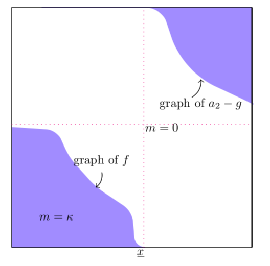
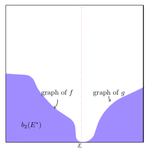
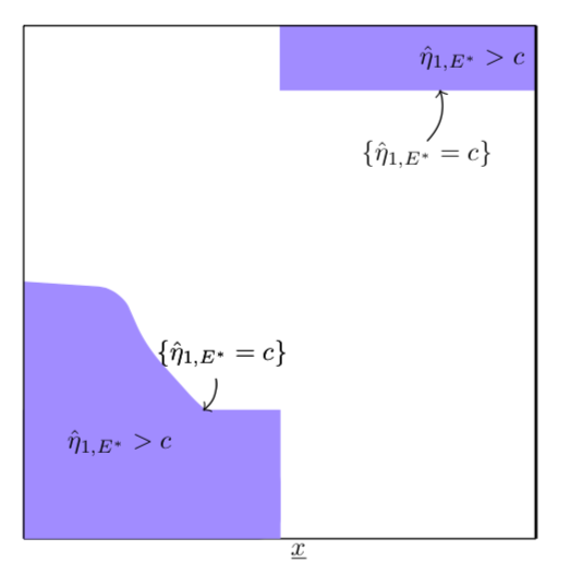
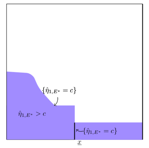
Figure 4: Illustration of the proof and the notations used.

2.5 Proof of Theorem 3

As a preliminary remark, we claim that the function $\theta_{\tilde{m},\mu}$ solving (LDE) with $m=\tilde{m}$ is positive increasing. Indeed, recall that $\theta_{\tilde{m},\mu}$ is the unique minimizer of the energy functional

$$\mathcal{E}:W^{1,2}({\Omega},\textrm{I\kern-2.10007ptR}_{+})\ni u\mapsto\frac{\mu}{2}\int_{0}^{1}u^{\prime 2}-\frac{1}{2}\int_{0}^{1}m^{*}u^{2}+\frac{1}{3}\int_{0}^{1}u^{3}.$$ (43)

By using the rearrangement inequalities recalled in Section 1.3 and the relation $(\tilde{m})_{br}=\tilde{m}$, one easily shows that

$$\mathcal{E}(\theta_{\tilde{m},\mu})\geqslant\mathcal{E}((\theta_{\tilde{m},\mu})_{br}),$$

and therefore, one has necessarily $\theta_{\tilde{m},\mu}=(\theta_{\tilde{m},\mu})_{br}$ by uniqueness of the steady-state (see Section 1.1). Hence, $\theta_{\tilde{m},\mu}$ is non-decreasing. Moreover, according to (LDE), $\theta_{\tilde{m},\mu}$ is convex on $(0,1-\ell)$ and concave on $(1-\ell,1)$ which, combined with the boundary conditions on $\theta_{\tilde{m},\mu}$, justifies the positiveness of its derivative. The expected result follows.

Step 1: convergence of sequences of maximizers.

As a consequence of Theorem 2, we get that the functions $\tilde{m}=\kappa\chi_{(0,\ell)}$ or $\tilde{m}(1-\cdot)=\kappa\chi_{(1-\ell,1)}$ are the only closure points of the family $(m_{\mu})_{\mu>0}$ for the $L^{1}(0,1)$ topology.

Step 2: asymptotic behaviour of $p_{m,\mu}$ and of ${\varphi}_{m,\mu}$

We claim that, as done for the solution $\theta_{m,\mu}$ of (LDE), the following asymptotic behaviour for the adjoint state $p_{m,\mu}$

$$p_{m,\mu}=-\frac{1}{m_{0}}+\underset{\mu\to\infty}{\operatorname{O}}(\frac{1}{\mu}),\quad\text{in }W^{2,2}(0,1),$$

by using Sobolev embeddings. In particular, this expansion holds in $\mathscr{C}^{1}([0,1])$.
Introduce the function $z_{\mu}=\mu(\varphi_{m_{\mu},\mu}+1)$. Using the convergence results established in the previous steps, in particular that $(m_{\mu})_{\mu>0}$ converges to $\tilde{m}$ in $L^{1}(0,1)$ and that $\varphi_{m_{\mu},\mu}=-1+\underset{\mu\to\infty}{\operatorname{O}}(\frac{1}{\mu})$ uniformly in $\mathscr{C}^{1,\alpha}([0,1])$ as $\mu\to+\infty$, one infers that $(z_{\mu})_{\mu>0}$ is uniformly bounded in $\mathscr{C}^{1,\alpha}([0,1])$ and converges, up to a subsequence to $z_{\infty}$ in $\mathscr{C}^{1}([0,1])$, where $z_{\infty}$ satisfies in particular

$$z_{\infty}^{\prime\prime}+2(m_{0}-\tilde{m})=0,$$

with Neumann Boundary conditions in the $W^{1,2}$ sense.

Conclusion: $m_{\mu}=\tilde{m}$ or $\tilde{m}(1-\cdot)$ whenever $\mu$ is large enough.

According to Theorem 1 and Proposition 3, we know at this step that for $\mu$ large enough, there exists $c_{\mu}\in\textrm{I\kern-2.10007ptR}$ such that

$$\{\varphi_{m_{\mu},\mu}>c_{\mu}\}=\{m_{\mu}=0\},\qquad\{\varphi_{m_{\mu},\mu}<c_{\mu}\}=\{m_{\mu}=\kappa\}.$$

We will show that, provided that $\mu$ be large enough, one has necessarily $m_{\mu}=\tilde{m}$ or $m_{\mu}=\tilde{m}(1-\cdot)$. Since $\tilde{m}=\kappa$ in $(0,\ell)$, it follows that $z_{\infty}$ is strictly convex on this interval and since $z_{\infty}^{\prime}(0)=0$, one has necessarily $z_{\infty}^{\prime}>0$ in $(0,\ell)$. Similarly, by concavity of $z_{\infty}$ in $(\ell,1)$, one has $z_{\infty}^{\prime}>0$ in this interval.

Furthermore, let us introduce $d_{\mu}=\mu(c_{\mu}+1)$. Since $(z_{\mu})_{\mu>0}$ is bounded in $C^{0}((0,1))$, $(d_{\mu})_{\mu>0}$ converges up to a subsequence to some $d_{\infty}$. By monotonicity of $z_{\infty}$ and a compactness argument, there exists a unique $x_{\infty}\in[0,\ell]$ such that $z_{\infty}(x_{\infty})=d_{\infty}$. The dominated convergence theorem hence yields

$$|\{z_{\infty}\leqslant d_{\infty}\}|=\kappa\ell,\qquad|\{z_{\infty}\geqslant d_{\infty}\}|=\kappa(1-\ell),$$

and the the aforementioned local convergence results yield

$$\{z_{\infty}>d_{\infty}\}\subset\{\tilde{m}=0\}\,,\quad\{z_{\infty}<d_{\infty}\}\subset\{\tilde{m}=\kappa\}.$$

Hence, the inclusions are equalities (the equality of sets must be understood up to a zero Lebesgue measure set) by using that $z_{\infty}$ is increasing.

Moreover, since $z_{\infty}$ is increasing, one has $z_{\infty}(0)<d_{\infty}$ and $z_{\infty}(1)>d_{\infty}$. Since the family $(z_{\mu})_{\mu>0}$ is uniformly Lipschitz-continuous, there exists ${\varepsilon}>0$ such that for $\mu$ large enough, there holds

$$z_{\mu}<d_{\mu}\hbox{ in }(0,{\varepsilon}),\quad z_{\mu}>d_{\mu}\hbox{ in }(1-{\varepsilon},1),\quad z_{\mu}^{\prime}>0\quad\hbox{ in }({\varepsilon},1-{\varepsilon}).$$

This implies the existence of $x_{\mu}\in(0,1)$ such that

$$\{z_{\mu}<d_{\mu}\}=[0,x_{\mu})\quad\hbox{and}\quad\{z_{\mu}>d_{\mu}\}=(x_{\mu},1],$$

whence the result.

2.6 Proof of Theorem 4

Let $\kappa>0,m_{0}>0$, and $\tilde{m}:=\kappa\chi_{[1-\ell,1)}$ with $\ell=\frac{m_{0}}{\kappa}$, i.e the single crenel distribution.
In order to prove this result, as the function $\mu>0\mapsto{\mathcal{F}_{\mu}}\left(\tilde{m}(2~{}\cdot)\right)$ has a first local maximizer ([31, Theorem 1.2, Remark 1.4]), we define $\mu_{1}$ as its first local maximizer. One gets from a simple change of variables that $\theta_{\tilde{m},\mu_{1}}(2x)=\theta_{\tilde{m}(2\cdot),\mu_{1}/4}(x)$ for all $x\in{\Omega}$ and thus one has

$$F_{\mu_{1}}(\tilde{m})={F}_{\frac{\mu_{1}}{4}}\left(\tilde{m}(2\cdot)\right)$$

But our choice of $\mu_{1}$ yields that $\mu\mapsto{\mathcal{F}_{\mu}}\left(\tilde{m}(2\cdot)\right)$ is increasing on $(0,\mu_{1})$ and thus:

$$F_{\mu_{1}}(\tilde{m})={F}_{\frac{\mu_{1}}{4}}\left(\tilde{m}(2\cdot)\right)<{F}_{\mu_{1}}\left(\tilde{m}(2\cdot)\right).$$ (44)

3 Conclusion and further comments

3.1 About the 1D case

Let us assume in this section that $n=1$ and $\Omega=(0,1)$. We provide hereafter several numerical simulations based on the primal formulation of the optimal design problem ($\mathcal{P}_{\mu}^{n}$): on Fig. 5, we investigate the general problem ($\mathcal{P}_{\mu}^{n}$) and we plot the optimal $m$ determined numerically for several values of $\mu$.

These simulations were obtained with an interior point method applied to the optimal control problem ($\mathcal{P}_{\mu}^{n}$). We used a Runge-Kutta method of order 4 to discretize the underlying differential equations. The control $m$ has been also discretized, which has allowed to reduce the optimal control problem to some finite dimensional minimization problem with constraints. We used the code IPOPT (see [42]) combined with AMPL (see [13]) on a standard desktop machine. We considered a regular subdivision of $(0,1)$ with $N$ points, where the order of magnitude of $N$ is $1000/\mu$. The resulting code works out the solution quickly (around 5 to 10 seconds depending on the choice of the parameter $\mu$).

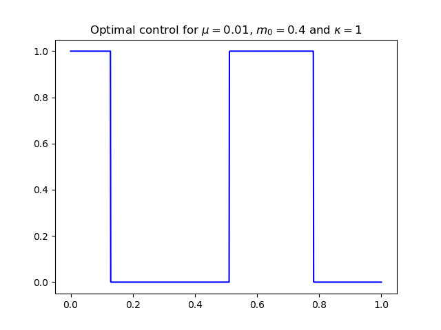
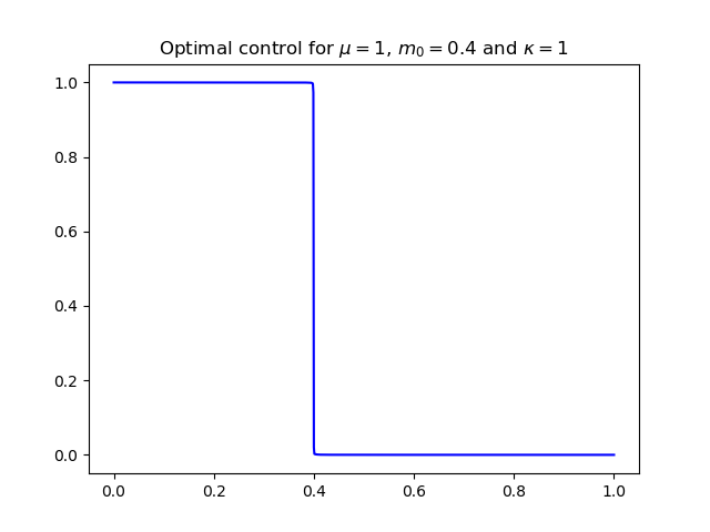
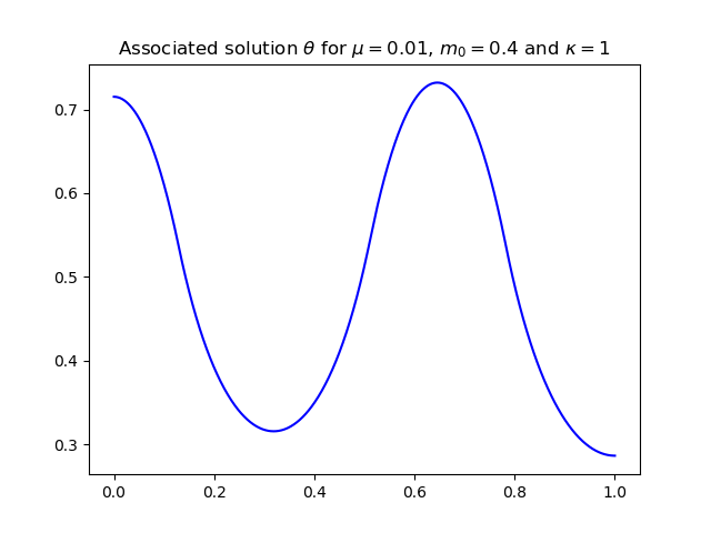
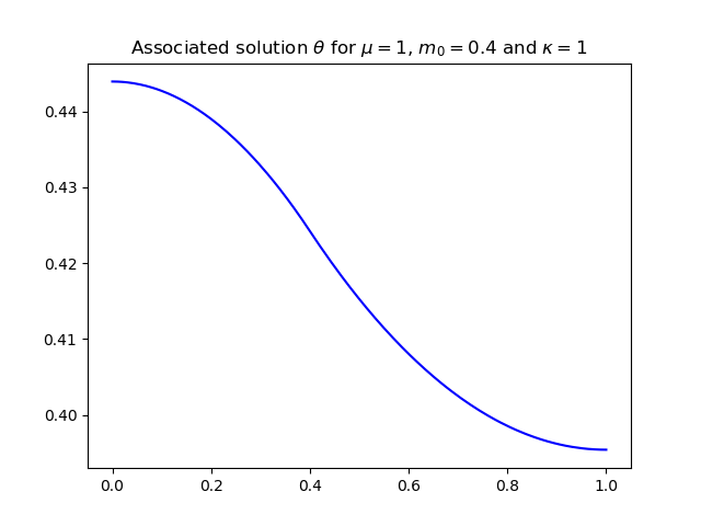
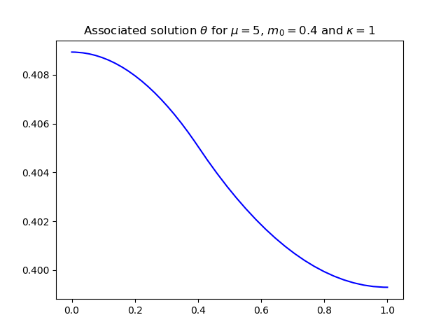
Figure 5: $m_{0}=0.4$, $\kappa=1$. From left to right: $\mu=0.01,1,5$. Top: plot of the optimal solution of Problem ($\mathcal{P}_{\mu}^{n}$) computed with the help of an interior point method. Bottom: plot of the corresponding eigenfunction.

In the cases mentioned above, the algorithm is initialized with several choices of function $m$, among which the optimal simple crenel as $\mu$ is large enough. If $\mu$ is equal to 1 or 5, the simple crenel is obtained at convergence. Nevertheless, in the case $\mu=0.01$, we obtain a “symmetric” double crenel (in accordance with Theorem 4) at convergence.

Although we have no guarantee to obtain optimal solutions by using this numerical approach, we checked that a simple crenel is better than a double one in the cases $\mu=1,\ 5$ whereas we observe the contrary in the case $\mu=0.01$.

Notice that we encountered a problem when dealing with too small values of $\mu$ (for instance $\mu=0.001$). Indeed, in that case, the stiffness of the discretized system seems to become huge as $\mu$ takes small positive values and makes the numerical computations hard to converge. Improvements of the numerical method should be found for further numerical investigations.

3.2 Comments and open issues

It is also interesting, from a biological point of view, to investigate a more general version of Problem ($\mathcal{P}_{\mu}^{n}$) for changing-sign weights. In that case, the admissible class of weights is then transformed (for instance) into

$$\widetilde{\mathcal{M}}_{m_{0},\kappa}({\Omega})=\left\{m\in L^{\infty}({\Omega})\,,m\in[-1;\kappa]\text{ a.e and }\fint_{\Omega}m=m_{0}\right\},$$

with $m_{0}\in(0,1)$ (so that $\lambda_{1}(m,\mu)>0$ and Equation (LDE) is well-posed). We claim that the main results of this article can be extended without effort to this new framework and that we will still obtain the bang-bang character of maximizers provided that $\mu$ be large enough. Such a class has also been considered in the context of principal eigenvalue minimization (see [18, 28]).

Finally, we end this section by providing some open problems for which we did not manage to bring complete answer and that deserve and remain, to our opinion, to be investigated. They are in order:

• (for general domains $\Omega$) we conjecture that maximizers are bang-bang functions for any $\mu>0$. As outlined in the introduction, this conjecture is supported by Theorem 1 and the main result of [36].

• (for general domains $\Omega$) use the main results of the present article to determine numerically the maximizer $m^{*}$ with the help of an adapted shape optimization algorithm;

• (for ${\Omega}=(0;1)$) given that, for $\mu$ small enough, the optimal configurations for $\lambda_{1}(\cdot,\mu)$ and ${\mathcal{F}_{\mu}}$ are not equal, it would be natural and biologically relevant to try to maximize a convex combination of ${\mathcal{F}_{\mu}}$ and $\lambda_{1}(\cdot,\mu)$.

• (for general domains $\Omega$) investigate the asymptotic behavior of maximizer as the parameter $\mu$ tends to 0? Such a issue appears intricate since it requires a refine study of singular limits for Problem (LDE).

Aknowledgements

The authors thank the reviewers for their thorough reviews and highly appreciate the comments and suggestions, which significantly contributed to improve the quality of the publication.

Appendix A Convergence of the series

Let $\frac{1}{\mu^{*}_{1}}$ be the minimum of the convergence radii associated to the power series $\sum\alpha(k)x^{k}$, $\sum\sigma(k)x^{k}$, $\sum\gamma(k)x^{k}$, $\sum\delta(k)x^{k}$ and $\sum\varepsilon(k)x^{k}$ introduced in the proof of Theorem 1.

We will show that, whenever $\mu\geqslant\mu^{*}_{1}$, the following expansions

$$\sum_{\ell=0}^{+\infty}\frac{{\eta_{k,m}}}{\mu^{k}}={\theta_{m,\mu}},\quad\sum_{k=1}^{+\infty}\frac{{\dot{\eta}_{k,m}}}{\mu^{k}}={\dot{\theta}_{m,\mu}},\quad\sum_{k=1}^{+\infty}\frac{\ddot{\eta}_{k,m}}{\mu^{k}}=\ddot{\theta}_{m,\mu}$$

make sense in ${L^{2}({\Omega})}$. Since the proofs for the series defining ${\dot{\theta}_{m,\mu}}$ and $\ddot{\theta}_{m,\mu}$ are exactly similar to the one for ${\theta_{m,\mu}}$, we only concentrate on the expansion of ${\theta_{m,\mu}}$. By construction, the series $g_{\infty,\mu}:=\sum_{\ell=0}^{+\infty}\frac{{\eta_{k,m}}}{\mu^{k}}$ converges in $W^{1,2}({\Omega})$ to a function $g_{\infty,\mu}$. We need to show that $g_{\infty,\mu}={\theta_{m,\mu}}$.

To this aim, let us set

$$g_{N,\mu}:=\sum_{k=0}^{N}\frac{{\eta_{k,m}}}{\mu^{k}}$$

for any $N\in\textrm{I\kern-2.10007ptN}^{*}$, Notice that $g_{N,\mu}$ solves the equation

$$\mu\Delta g_{N,\mu}+g_{N-1,\mu}m-\sum_{k=0}^{N}\frac{\eta_{k,m}}{\mu^{k}}g_{N-k,\mu}=0,\quad\text{in }{\Omega}$$ (45)

with Neumann boundary conditions.

In order to pass to the limit $N\to\infty$, one has to determine the limit of $\tilde{g}_{N,\mu}:=\sum_{k=0}^{N}\frac{\eta_{k,m}}{\mu^{k}}g_{N-k,\mu}$. First note that the Cauchy-Schwarz inequality proves the absolute convergence of the sequence $\left\{\tilde{g}_{N,\mu}\right\}_{N\in\textrm{I\kern-1.47005ptN}}$ in $W^{1,2}({\Omega})$ as $N\to\infty$. Let $H$ denote its limit. Now, let us show that

$$\tilde{g}_{N,\mu}\underset{N\to\infty}{\to}g_{\infty,\mu}^{2}\quad\text{ in }L^{2}({\Omega}),$$

whenever $\mu$ is large enough. Let $R_{1}$ be the convergence radius of the power series associated with the sequence $\{\alpha(k)\}_{k\in\textrm{I\kern-1.47005ptN}}$. This convergence radius is known to be positive. As a consequence, the convergence radius $R_{2}$ of the power series associated with the sequence $\{\alpha(k)^{2}\}_{k\in\textrm{I\kern-1.47005ptN}}$ is also positive and $R_{2}=R_{1}^{2}.$

Let ${\varepsilon}>0$. Since we are only working with large diffusivities, let us assume that $\mu\geqslant 1$ and that $\mu>(\frac{1}{R_{2}})^{1/{\varepsilon}}.$ Noting that, for any $N\in\textrm{I\kern-2.10007ptN}$, we have

$$\tilde{g}_{N,\mu}-g_{N,\mu}^{2} =\sum_{k=0}^{N}\frac{1}{\mu^{k}}\eta_{k,m}\left(\sum_{\ell=N-k+1}^{N}\frac{\eta_{\ell,m}}{\mu^{\ell}}\right).$$

and using the fact that the sequence $\{\alpha(k)\}_{k\in\textrm{I\kern-1.47005ptN}}$ was built increasing, we get the existence of $M>0$ such that

$$\frac{1}{|\Omega|}\|\tilde{g}_{N,\mu}-g_{N,\mu}^{2}\|_{L^{2}({\Omega})} =\frac{1}{|\Omega|}\Bigg{\|}\sum_{k=0}^{N}\frac{1}{\mu^{k}}\eta_{k,m}\left(\sum_{\ell=N-k+1}^{N}\frac{\eta_{\ell,m}}{\mu^{\ell}}\right)\Bigg{\|}_{L^{2}({\Omega})}$$

$$\leqslant\sum_{k=0}^{N}\frac{\alpha(k)}{\mu^{k}}\left(\sum_{\ell=N-k+1}^{N}\frac{\alpha({\ell})}{\mu^{\ell}}\right)$$

$$\leqslant\alpha(N)^{2}\sum_{k=0}^{N}\frac{1}{\mu^{k}}\left(\frac{1}{\mu^{N-k+1}}\frac{1-\frac{1}{\mu^{k-1}}}{1-\frac{1}{\mu}}\right) \text{ by using that }\alpha(k)\alpha(\ell)\leqslant\alpha(N)^{2}$$

$$\leqslant M\frac{(N+1)\alpha(N)^{2}}{\mu^{N+1}}$$

$$=M\frac{N+1}{(\mu^{1-{\varepsilon}})^{N+1}}\frac{\alpha(N)^{2}}{(\mu^{\varepsilon})^{N+1}}.$$

This last quantity converges to zero as $N\to\infty$. Besides, since $\mu^{\varepsilon}\geqslant\frac{1}{R_{2}}$, it follows that the sequence $\left\{\frac{\alpha(N)^{2}}{(\mu^{\varepsilon})^{N+1}}\right\}_{N\to\infty}$ is bounded. Assuming moreover that $\mu^{1-{\varepsilon}}>1$, we get

$$\frac{N+1}{(\mu^{1-{\varepsilon}})^{N+1}}\xrightarrow[N\to\infty]{}0.$$

We conclude that $H=g_{\infty,\mu}^{2}$. Passing to the limit in Equation (45), it follows that

$$\mu\Delta g_{\infty,\mu}^{2}+g_{\infty,\mu}(m-g_{\infty,\mu})=0\quad\text{in }{\Omega}$$

with Neumann boundary conditions.

Finally, we know that $g_{\infty,\mu}\underset{\mu\rightarrow+\infty}{\rightarrow}m_{0}$ uniformly in $\mathcal{M}_{m_{0},\kappa}({\Omega})$ and moreover, one has $m_{0}>0$. It follows that, for $\mu$ large enough, $g_{\infty,\mu}$ is positive. The uniqueness of positive solutions of equation (LDE) entails that, for $\mu$ large enough, $g_{\infty,\mu}={\theta_{m,\mu}}$. This concludes the proof of the series expansion convergences and thus, the proof of Theorem 1.

References

- [1] X. Bai, X. He, and F. Li. An optimization problem and its application in population dynamics. Proc. Amer. Math. Soc., 144(5):2161–2170, May 2016.
- [2] H. Berestycki, F. Hamel, and L. Roques. Analysis of the periodically fragmented environment model : I – species persistence. Journal of Mathematical Biology, 51(1):75–113, 2005.
- [3] H. Berestycki and T. Lachand-Robert. Some properties of monotone rearrangement with applications to elliptic equations in cylinders. Math. Nachr., 266:3–19, 2004.
- [4] H. Brezis. Functional Analysis, Sobolev Spaces and Partial Differential Equations. Springer New York, 2010.
- [5] R. Cantrell and C. Cosner. Diffusive logistic equations with indefinite weights: population models in disrupted environments. II. SIAM J. Math. Anal., 22(4):1043–1064, 1991.
- [6] R. S. Cantrell and C. Cosner. The effects of spatial heterogeneity in population dynamics. J. Math. Biol., 29(4):315–338, 1991.
- [7] R. S. Cantrell and C. Cosner. Spatial Ecology via Reaction-Diffusion Equations. John Wiley & Sons, 2003.
- [8] A. Cianchi and V. G. Maz’ya. Global lipschitz regularity for a class of quasilinear elliptic equations. Communications in Partial Differential Equations, 36(1):100–133, 2010.
- [9] W. Ding, H. Finotti, S. Lenhart, Y. Lou, and Q. Ye. Optimal control of growth coefficient on a steady-state population model. Nonlinear Analysis: Real World Applications, 11(2):688 – 704, 2010.
- [10] J. Dockery, V. Hutson, K. Mischaikow, and M. Pernarowski. The evolution of slow dispersal rates: a reaction diffusion model. Journal of Mathematical Biology, 37(1):61–83, 1998.
- [11] A. Ferone and R. Volpicelli. Minimal rearrangements of sobolev functions: a new proof. Annales de l’Institut Henri Poincaré, 20:333–339, 2003.
- [12] R. A. Fisher. The wave of advance of advantageous genes. Annals of Eugenics, 7(4):355–369, 1937.
- [13] R. Fourer. AMPL : a modeling language for mathematical programming. San Francisco, Calif. : Scientific Pr., San Francisco, Calif., 2. ed. edition, 1996.
- [14] X. He and W.-M. Ni. Global dynamics of the Lotka–Volterra competition–diffusion system with equal amount of total resources, III. Calc. Var. Partial Differential Equations, 56(5):56:132, 2017.
- [15] A. Henrot and M. Pierre. Variation et optimisation de formes, volume 48. Springer-Verlag Berlin Heidelberg, 2005.
- [16] P. Hess. Periodic-parabolic boundary value problems and positivity, volume 247 of Pitman Research Notes in Mathematics Series. Longman Scientific & Technical, Harlow; copublished in the United States with John Wiley & Sons, Inc., New York, 1991.
- [17] P. Hess and T. Kato. On some linear and nonlinear eigenvalue problems with an indefinite weight function. Comm. Partial Differential Equations, 5(10):999–1030, 1980.
- [18] M. Hintermüller, C.-Y. Kao, and A. Laurain. Principal eigenvalue minimization for an elliptic problem with indefinite weight and Robin boundary conditions. Appl. Math. Optim., 65(1):111–146, 2012.
- [19] K. Jha and G. Porru. Minimization of the principal eigenvalue under Neumann boundary conditions. Numer. Funct. Anal. Optim., 32(11):1146–1165, 2011.
- [20] C.-Y. Kao, Y. Lou, and E. Yanagida. Principal eigenvalue for an elliptic problem with indefinite weight on cylindrical domains. Math. Biosci. Eng., 5(2):315–335, 2008.
- [21] T. Kato. Perturbation theory for linear operators. Classics in Mathematics. Springer-Verlag, Berlin, 1995. Reprint of the 1980 edition.
- [22] K. Kawasaki and N. Shigesada. Biological Invasions: Theory And Practice, volume 66. Oxford University Press, 11 1997.
- [23] K. Kawasaki, N. Shigesada, and E. Teramoto. Traveling periodic waves in heterogeneous environments. Theoretical Population Biology, 30(1):143–160, Aug. 1986.
- [24] B. Kawohl. Rearrangements and convexity of level sets in PDE, volume 1150 of Lecture Notes in Mathematics. Springer-Verlag, Berlin, 1985.
- [25] B. Kawohl. On the isoperimetric nature of a rearrangement inequality and its consequences for some variational problems. Archive for Rational Mechanics and Analysis, 94(3):227–243, 1986.
- [26] N. Kinezaki, K. Kawasaki, N. Shigesada, and F. Takasu. Biological Invasion into Periodically Fragmented Environments: A Diffusion-Reaction Model, pages 215–222. 01 2003.
- [27] A. Kolmogorov, I. Pretrovski, and N. Piskounov. étude de l’équation de la diffusion avec croissance de la quantité de matière et son application à un problème biologique. Moscow University Bulletin of Mathematics, 1:1–25, 1937.
- [28] J. Lamboley, A. Laurain, G. Nadin, and Y. Privat. Properties of optimizers of the principal eigenvalue with indefinite weight and Robin conditions. Calc. Var. Partial Differential Equations, 55(6):55:144, 2016.
- [29] E. Lieb and M. Loss. Analysis. American Mathematical Society, 2001.
- [30] J.-L. Lions and E. Magenes. Problemi ai limiti non omogenei (iii). Annali della Scuola Normale Superiore di Pisa - Classe di Scienze, Ser. 3, 15(1-2):41–103, 1961.
- [31] Y. Lou. On the effects of migration and spatial heterogeneity on single and multiple species. Journal of Differential Equations, 223(2):400 – 426, 2006.
- [32] Y. Lou. Tutorials in Mathematical Biosciences IV: Evolution and Ecology, chapter Some Challenging Mathematical Problems in Evolution of Dispersal and Population Dynamics, pages 171–205. Springer Berlin Heidelberg, Berlin, Heidelberg, 2008.
- [33] Y. Lou and E. Yanagida. Minimization of the principal eigenvalue for an elliptic boundary value problem with indefinite weight, and applications to population dynamics. Japan J. Indust. Appl. Math., 23(3):275–292, 2006.
- [34] D. Ludwig, D. G. Aronson, and H. F. Weinberger. Spatial patterning of the spruce budworm. Journal of Mathematical Biology, 8(3):217–258, 1979.
- [35] I. Mazari. Trait selection and rare mutations steady-state models for large diffusivities. Discrete and continuous dynamical systems, Series B, 2019 (Accepted for publication).
- [36] K. Nagahara and E. Yanagida. Maximization of the total population in a reaction–diffusion model with logistic growth. Calculus of Variations and Partial Differential Equations, 57(3):80, Apr 2018.
- [37] J.-M. Rakotoson. Réarrangement relatif, volume 64 of Mathématiques & Applications (Berlin) [Mathematics & Applications]. Springer, Berlin, 2008. Un instrument d’estimations dans les problèmes aux limites. [An estimation tool for limit problems].
- [38] S. Roman. An Introduction to Catalan Numbers. Compact Textbooks in Mathematics. Springer International Publishing, 2015.
- [39] L. Roques and F. Hamel. Mathematical analysis of the optimal habitat configurations for species persistence. Math. Biosci., 210(1):34–59, 2007.
- [40] J. G. Skellam. Random dispersal in theoretical populations. Biometrika, 38:196–218, 1951.
- [41] G. Stampacchia. Le problème de dirichlet pour les équations elliptiques du second ordre à coefficients discontinus. Annales de l’Institut Fourier, 15(1):189–257, 1965.
- [42] A. Wächter and L. T. Biegler. On the implementation of an interior-point filter line-search algorithm for large-scale nonlinear programming. Math. Program., 106(1, Ser. A):25–57, 2006.
- [43] J. M. Yong and P. J. Zhang. Necessary conditions of optimal impulse controls for distributed parameter systems. Bull. Austral. Math. Soc., 45(2):305–326, 1992.