Exact WKB analysis of $\mathbb{CP}^{1}$ holomorphic blocks

Abstract

We study holomorphic blocks in the three dimensional ${\mathcal{N}}=2$ gauge theory that describes the $\mathbb{CP}^{1}$ model. We apply exact WKB methods to analyze the line operator identities associated to the holomorphic blocks and derive the analytic continuation formulae of the blocks as the twisted mass and FI parameter are varied. The main technical result we utilize is the connection formula for the ${}_{1}\phi_{1}$ $q$-hypergeometric function. We show in detail how the $q$-Borel resummation methods reproduce the results obtained previously by using block-integral methods.

1 Introduction and summary

Three-dimensional supersymmetric gauge theories are known to exhibit interesting dynamics, such as mirror symmetry, and IR dualities Intriligator:1996ex ; Aharony:1997bx ; Dorey:1999rb ; Tong:2000ky . With the application of localization methods Witten:1988ze ; Pestun:2007rz to these theories on (squashed) $S^{3}$ Kapustin:2009kz ; Jafferis:2010un ; Hama:2010av ; Hama:2011ea ; Imamura:2011wg ; Nian:2013qwa , it became possible to compute their exact partition functions and other supersymmetric observables. This opened up new avenues to further delve into the rich dynamics of these theories and uncover possibly new symmetries and dualities, including holography (see chapters 6-8 of Pestun:2016jze and references therein). A new perspective on computing these partition functions was discovered shortly afterwards Pasquetti:2011fj ; Dimofte:2011py in terms of holomorphic blocks. They were then extensively studied in Beem:2012mb as fundamental objects using which the partition functions and (twisted) indices of these 3d gauge theories can be obtained by gluing these blocks in distinct ways. These have proved useful in understanding mirror symmetry and discovering more dualities (see, for example, Zenkevich:2017ylb ; Aprile:2018oau ). The factorization into holomorphic blocks have been shown for partition functions on more general 3-manifolds Imamura:2013qxa ; Nieri:2015yia ; Closset:2017zgf ; Closset:2018ghr ; Pittelli:2018rpl . They have also played a key role in the 3d/3d correspondence in which they were mapped to partition functions of complex Chern-Simons theories on Lefschetz thimbles Witten:2010cx ; Dimofte:2010tz ; Witten:2010zr ; Witten:2011zz ; Dimofte:2011ju . The 3d holomorphic blocks are also related to 4d and 5d theories where such a factorization of partition functions is again observed Yoshida:2014qwa ; Nieri:2015yia ; Pasquetti:2016dyl ; Longhi:2019hdh .

One of the main properties of the 3d holomorphic blocks that we focus on in this paper is that they are solutions to $q$-difference equations. These are referred to as line operator identities (LOIs) in Beem:2012mb and can be derived systematically given the ultraviolet description of the gauge theory. Another important property of interest to physical applications is that these blocks exhibit Stokes phenomena as the parameters of the gauge theory are varied. The physical parameters are the complexified masses and FI parameters of the gauge theory. The parameter space is divided up into Stokes regions and in each such region, the LOIs have as many independent solutions as the number of massive vacua of the gauge theory. Since the blocks solve linear difference equations, in each Stokes region the holomorphic blocks form a basis; this basis can be written as a linear combination of the basis in the neighbouring Stokes regions. The Stokes matrices/multipliers give the relation between these bases defined in the Stokes regions separated by a Stokes line. In Beem:2012mb , it was also shown that the holomorphic blocks could be written as finite dimensional contour integrals (termed block-integrals) such that they automatically solve the LOIs. The Stokes phenomenon exhibited by the holomorphic blocks was then shown to be a consequence of a change of contours as the Stokes lines are crossed.

In this work, we approach the same problem from a purely algebraic perspective and show that the Stokes behaviour of the blocks can be obtained by analyzing the exact WKB properties of the $q$-difference equations that are satisfied by the holomorphic blocks (see RSZ for an introduction to $q$-difference equations). We focus on the $\mathbb{CP}^{1}$ model Witten:1993yc ; Dorey:1999rb ; Tong:2000ky , which has a gauge theory description in the ultraviolet as a U$(1)$ gauge theory with two charged chiral multiplets. This is the simplest model in which the LOIs have an irregular singular point, in addition to a regular singular point TAB . Up to prefactors that are given in terms of $\Theta_{q}$-functions, the blocks near the regular singular point are given in terms of the $q$-hypergeometric function ${}_{1}\phi_{1}(0;a;q,z)$.

We cannot directly solve these LOIs near the irregular singular point and have to turn to connection formulae, which relate solutions of $q$-difference equations near different singular points. However, the well-known connection formulae Watson:1910ghs relate the solutions near two regular singularities. Whereas these solutions have finite radius of convergence, solutions around an irregular singularity are typically asymptotic series with zero radius of convergence. To extend the connection formulae to solutions near irregular singularities, one has to augment the procedure by first carrying out the $q$-Borel summation Morita:2011hx ; MOR ; DRELO ; OHY ; OHYtalk ; Adachi of the asymptotic series near the irregular singular point. These methods have been applied to the study of the connection formula for ${}_{1}\phi_{1}$-function in $|q|<1$ chamber but we also need the connection formula in the $|q|>1$ chamber to completely characterize the Stokes phenomena exhibited by $\mathbb{CP}^{1}$ model. One of the main technical results of this work is a derivation of the $|q|>1$ formula suitably adapting the treatment of the $|q|<1$ result in OHY .

An important subtlety in the derivation of the connection formulae is that the analytic continuation of the ${}_{1}\phi_{1}$-function in fact depends on the choice of an arbitrary complex number $\lambda$. Naively it would appear as if there is a one-parameter family of analytically continued holomorphic blocks. However, there are two independent LOIs in the $\mathbb{CP}^{1}$ model and it turns out that it is only for two particular choices of $\lambda$, determined by the physical parameters of the theory, that the analytic continuation leads to consistent holomorphic blocks. So, in the end, this procedure leads to three pairs of $\mathbb{CP}^{1}$ blocks (one set near the regular singular point and two sets near the irregular singular point) and each of these pairs correspond to a basis in a particular Stokes region in the parameter space. These correctly reproduce the expected Stokes behaviour of the $\mathbb{CP}^{1}$ blocks, derived from the block-integral analysis in Beem:2012mb .

This paper is organized as follows: In Section 2 we review the $q$-Borel and $q$-Laplace transforms to solve the $q$-difference equations. In Section 3 we review the $\mathbb{CP}^{1}$ model, obtain the holomorphic blocks near the regular singular point by solving the LOIs explicitly, and briefly review the results of Beem:2012mb . Then in Section 4 we apply the results of Section 2 to write down the connection formulae that relate holomorphic blocks in the different Stokes regions. Finally, in Section 5 we bring all the results together to identify the pair of holomorphic blocks in each Stokes region along with explicitly identifying the relevant regions in the parameter space of the $\mathbb{CP}^{1}$ model. We also have three technical appendices, including the detailed derivation of the connection formula in $|q|>1$ chamber for the ${}_{1}\phi_{1}$-function in Appendix C.

2 $\bm{q}$-Borel resummation for $\bm{q}$-difference equations

Our goal in this work is to study holomorphic blocks in various regions of parameter space and to analyze how these blocks behave as one crosses Stokes lines in the parameter space using purely algebraic techniques. The holomorphic blocks obey line operator identities, which are a set of $q$-difference equations. In this section, following MOR ; OHY , we review the $q$-Borel resummation methods that allow one to eventually solve the connection problem of analytically continuing solutions of $q$-difference equations around an irregular singular point to solutions around a regular singular point.

2.1 The $\bm{q}$-Borel transform

We begin with a $q$-difference equation of the form

$${\mathcal{D}}[\sigma_{q}(t)]\,f(t)=0\,,$$ (2.1)

where $\sigma_{q}(t)=q^{t\frac{d}{dt}}$ such that $\sigma_{q}(t)f(t)=f(qt)$ and we look for solutions near the point $t=0$. The $q$-Borel resummation involves two steps: i) $q$-Borel transform followed by ii) its inverse, the $q$-Laplace transform. The $q$-Borel transform of a formal series $f(t)=\sum_{n=0}a_{n}t^{n}$ is defined for both $|q|\gtrless 1$ as follows:

$$\mathcal{B}^{\pm}_{q}[f(t)](\tau)=\sum_{n=0}^{\infty}a_{n}q^{\pm\frac{n}{2}(n-1)}\tau^{n}\,.$$ (2.2)

In what follows, we will apply this operator to the $q$-difference equation and the following result will prove useful:

$$\mathcal{B}^{\pm}_{q}\left[t^{m}\sigma^{p}_{q}(t)f(t)\right](\tau)=q^{\pm\frac{m}{2}(m-1)}\tau^{m}\sigma_{q}^{p\pm m}(\tau)\mathcal{B}^{\pm}_{q}[f(t)](\tau)\,.$$ (2.3)

2.2 The $\bm{q}$-Laplace transform

After acting with the $q$-Borel transform on a divergent solution around an irregular singular point, we use the inverse transform to get the actual solution. There are two types of $q$-Borel transforms and there are correspondingly two types of inverse transforms which we discuss in turn, following OHY . We will also see in the following sections that as the theta function $\Theta_{q}(x)$ has different series expansion for different $|q|$ chambers, we have to use different $q$-Laplace transforms in the corresponding $q$-chambers.

2.2.1 The $\bm{q}$-Laplace transform $\bm{\mathcal{L}_{q}^{-}}$ for $\bm{|q|<1}$

We define the $q$-Laplace transform $\mathcal{L}_{q}^{-}$ to be given by the contour integral OHY :

$$\mathcal{L}_{q}^{-}[f(t)](\tau)=\frac{1}{2\pi i}\oint_{\Gamma_{\epsilon}}\frac{ds}{s}f(s)\Theta_{q}\left(\tau s^{-1}\right),$$ (2.4)

where the contour $\Gamma_{\epsilon}$ is a circle of small radius $\epsilon$ in the complex $s$-plane around $s=0$ and the $\Theta_{q}$-function is defined in Appendix B. Consider the action of this operation on a convergent power series $g(z)$. Any such power series is written in the form:

$$g(z)=\sum_{n\geq 0}a_{n}b_{n}z^{n}\,.$$ (2.5)

If the series has a finite radius of convergence (say $r$), it can be re-expressed in terms of the following integral (using Cauchy’s residue theorem):

$$\sum_{n\geq 0}a_{n}b_{n}z^{n}=\frac{1}{2\pi i}\oint_{\Gamma_{\epsilon}}\frac{ds}{s}\alpha(s)\beta\left(zs^{-1}\right),$$ (2.6)

where $\alpha(s)=\sum_{n\geq 0}a_{n}s^{n}$ and $\beta(zs^{-1})=\sum_{m\geq 0}b_{m}(zs^{-1})^{m}$. If $\alpha(s)$ and $\beta(s)$ are two convergent series with maximum radius of convergence $r$, then we see that equation (2.6) holds.

Let us now set

$$\alpha(s)=\mathcal{B}_{q}^{-}[f(t)](s)\quad\text{ and }\quad\beta\left(zs^{-1}\right)=\Theta_{q}\left(-zs^{-1}\right),$$ (2.7)

and calculate the r.h.s of (2.6):

$$\frac{1}{2\pi i}\oint_{\Gamma_{\epsilon}}\frac{ds}{s}\sum_{n\geq 0}\sum_{m\in\mathbb{Z}}a_{n}q^{-\frac{n}{2}(n-1)}q^{\frac{m}{2}(m-1)}z^{m}s^{n-m}\,.$$ (2.8)

In the last summation one can restrict the values in the summation over $m$ to those with $m\geq 0$ as the $m\leq-1$ values do not give rise to poles. Hence, for $m,n\geq 0$ the non-zero contributions arise only from the case $n=m$ (as all higher order residues are vanishing), which lead to the following result:

$$\frac{1}{2\pi i}\oint_{\Gamma_{\epsilon}}\frac{ds}{s}\mathcal{B}_{q}^{-}[f(t)](s)\Theta_{q}\left(-zs^{-1}\right)=\sum_{n\geq 0}a_{n}z^{n}=f(z)\,.$$ (2.9)

So, we find the $q$-Laplace transform defined in (2.4) inverts the $q$-Borel transform ${\mathcal{B}}^{-}_{q}$ for convergent power series:

$$(\mathcal{L}_{q}^{-}\circ\mathcal{B}^{-}_{q})[f]=f\,.$$ (2.10)

While applying this formalism to find the holomorphic blocks of the $\mathbb{CP}^{1}$ model, we will begin with a particular ansatz for the solution of a $q$-difference equation that involves factoring out $\Theta_{q}$-function (or its inverse) from a formal power series (see (4.2), (4.3)). Then, applying the $q$-Borel transform to this power series, we will see that ${\mathcal{B}}_{q}^{-}[f](s)$ has simple poles in the $s$-plane. Applying the $q$-Laplace transform ${\mathcal{L}}^{-}_{q}$ as defined in (2.4), we shall see that deforming the contour to pick up these poles gives rise to a connection formula.

2.2.2 The $\bm{q}$-Laplace transform $\bm{\mathcal{L}_{q,\lambda}^{+}}$ for $\bm{|q|<1}$

The $q$-Laplace transform of type $+$ is defined as follows OHY :

$$\mathcal{L}_{q,\lambda}^{+}[f(\tau)](t)=\sum_{m\in\mathbb{Z}}\frac{f(\lambda q^{m})}{\Theta_{q}\left(-\lambda q^{m}t^{-1}\right)}\,\cdot$$ (2.11)

Note that this transform depends on an extra complex parameter $\lambda$. With this definition one can show that both $q$-Borel and $q$-Laplace transforms are additive under addition of different functions. Using this fact we can show that

$$(\mathcal{L}_{q,\lambda}^{+}\circ\mathcal{B}_{q}^{+})[f]=f\,,$$ (2.12)

where $f(x)$ is convergent. We present the inductive proof following OHY . First we note that

$$\mathcal{L}_{q,\lambda}^{+}[1](t)=\sum_{m\in\mathbb{Z}}\frac{1}{\Theta_{q}\left(-\lambda q^{m}t^{-1}\right)}=\frac{1}{\Theta_{q}\left(-\lambda t^{-1}\right)}\sum_{m\in\mathbb{Z}}\lambda^{m}t^{-m}q^{\frac{m}{2}(m-1)}=1\,.$$ (2.13)

We always set $a_{0}=1$ in formal series so that we can have

$$\mathcal{B}^{+}_{q}[1](\tau)=1\,.$$ (2.14)

Now we assume that

$$\mathcal{L}_{q,\lambda}^{+}\big{[}\mathcal{B}^{+}_{q}[a\,z^{n}](\tau)\big{]}(t)=a\,t^{n}\,.$$ (2.15)

By noting the following relation:

$$\mathcal{B}^{+}_{q}\big{[}a\,z^{n+1}\big{]}(\tau)=q^{n}\tau\mathcal{B}^{+}_{q}[a\,z^{n}](\tau)\,,$$ (2.16)

one can show that

$$\mathcal{L}_{q,\lambda}^{+}\big{[}\mathcal{B}^{+}_{q}\big{[}a\,z^{n+1}\big{]}(\tau)\big{]}(t)=a\,t^{n+1}\,.$$ (2.17)

Thus, if the function $f(t)=\sum_{n}a_{n}t^{n}$ with ($a_{0}=1)$ is convergent then we have a proof of (2.12). The key point to note here is the choice of a complex number $\lambda$ in the definition of the $q$-Laplace transform OHY ; DRELO . We first denote by $[\lambda]$ an equivalence class of $\lambda$ in $\mathbb{C}^{\star}/q^{\mathbb{Z}}$. We now have the constraint $\left[\lambda\right]\in\left(\mathbb{C}^{\star}/q^{\mathbb{Z}}\right)\setminus\{\left[1\right]\}$ since if $\lambda$ is an integral power of $q$, the definition in (2.11) leads to a divergent result. The choice of $\lambda$ will prove to be important in providing different ways to analytically continue the holomorphic blocks.

2.2.3 The $\bm{q}$-Laplace transform $\bm{\mathcal{L}_{q}^{+}}$ for $\bm{|q|>1}$

We define this $q$-Laplace transform for $|q|>1$ as follows

$$\mathcal{L}_{q}^{+}[f(t)](\tau)=\frac{1}{2\pi i}\oint_{\Gamma_{\epsilon}}\frac{ds}{s}f(s)\Theta_{q}^{-1}\left(-q\tau s^{-1}\right).$$ (2.18)

Notice that this definition follows naturally from the definition (2.4) for $|q|<1$, in view of the following transformation property of theta function

$$\Theta_{q}(x)=\Theta_{q^{-1}}^{-1}(x^{-1})\,.$$ (2.19)

This definition is consistent since the theta function has the following series expansion for $|q|>1$:

$$\Theta_{q}^{-1}\left(-q\tau s^{-1}\right)=\sum_{n\in\mathbb{Z}}q^{-\frac{n}{2}(n-1)}\left(\tau s^{-1}\right)^{n}\,.$$ (2.20)

We denote this $q$-Laplace transform as $\mathcal{L}_{q}^{+}$ because now it satisfies

$$(\mathcal{L}_{q}^{+}\circ\mathcal{B}_{q}^{+})[f]=f\,.$$ (2.21)

2.2.4 The $\bm{q}$-Laplace transform $\bm{\mathcal{L}_{q,\lambda}^{-}}$ for $\bm{|q|>1}$

The $q$-Laplace transform of type $-$ for $|q|>1$ can be defined as follows:

$$\mathcal{L}_{q,\lambda}^{-}[f(\tau)](t)=\sum_{m\in\mathbb{Z}}f(\lambda q^{m})\,\Theta_{q}\left(-\lambda q^{m+1}t^{-1}\right).$$ (2.22)

Its consistency can again be checked by following the previous analysis for $|q|<1$.

3 The $\bm{\mathbb{CP}^{1}}$ model

We now turn to the prototypical theory in which holomorphic blocks exhibit Stokes phenomena. The $\mathbb{CP}^{1}$ model can be described in the ultraviolet as a gauged linear sigma model (GLSM) Witten:1993yc that flows, in the infrared, to a non-linear sigma model with target space $\mathbb{CP}^{1}$. The GLSM is a U$(1)$ gauge theory with two chiral fields $(\phi_{1},\phi_{2})$ that have same charges under the U$(1)$ gauge group. The theory has a flavour symmetry SU$(2)\times$U$(1)_{J}$ as well as a U$(1)_{R}$ symmetry. The flavour symmetry is broken to U$(1)_{V}\times$U$(1)_{J}$ by a twisted mass $m$ for the fundamental flavours. Similarly, we associate the FI parameter $t$ to the U$(1)_{J}$ symmetry. The scalar $\sigma$ in the vector multiplet is complexified by the Wilson line for the gauge field to a field we denote $S$. The twisted mass $m$ and FI parameter $t$ are similarly complexified to $X$ and $Y$ by Wilson lines for the global U$(1)$ symmetries, respectively. As far as the 3d theory is concerned, the relevant variables and parameters are the exponentiated ones that we denote as follows:

$$s=e^{S}\,,\qquad x=e^{X}\,,\qquad y=e^{Y}\,.$$ (3.1)

We assign the following charges and Chern-Simons coefficients Beem:2012mb :

$$T^{\mathbb{CP}^{1}}[\vec{\phi}]=\left\{\quad\begin{array}[]{c|cc}Q&\phi_{1}&\phi_{2}\\ \hline\cr G&1&1\\ V&1&-1\\ J&0&0\\ R&0&0\end{array}\qquad\begin{array}[]{c|cccc}k&G&V&J&R\\ \hline\cr G&0&0&1&0\\ V&0&0&0&0\\ J&1&0&0&0\\ R&0&0&0&\star\end{array}\right.$$ (3.2)

Given this data, there is a systematic procedure described in Beem:2012mb to derive an integral representation for the holomorphic blocks and the line operator identities satisfied by the block. Since this is well-known, we simply state the result for the LOIs satisfied by the holomorphic blocks:

$$\widehat{p}_{y}+(\widehat{y}^{-1}-\widehat{x}-\widehat{x}^{-1})+\widehat{p}_{y}^{-1} \simeq 0\,,$$ (3.3)

$$q^{-\frac{1}{2}}\widehat{p}_{x}\widehat{p}_{y}-\widehat{x}\big{(}q^{\frac{1}{2}}\widehat{p}_{x}+\widehat{p}_{y}\big{)}+1 \simeq 0\,.$$ (3.4)

Here we have defined the operators $\widehat{p}_{x}=\sigma_{q}(x)$ and $\widehat{p}_{y}=\sigma_{q}(y)$, which satisfy the $q$-commutation relations $\widehat{p}_{x}\widehat{x}=q\,\widehat{x}\widehat{p}_{x}$ and $\widehat{p}_{y}\widehat{y}=q\,\widehat{y}\widehat{p}_{y}$.

Let us first review the results of Beem:2012mb in which the Stokes phenomenon is derived by making use of the block-integral representation for the holomorphic blocks. This analysis is restricted to the mirror symmetry invariant plane in the complex $(X,Y)$ parameter space, given by $\text{Im}(X)=-\frac{2\pi}{3}$ and $\text{Im}(Y)=0$. There are three Stokes regions and in each region, there are two solutions $({\mathbb{B}}^{1},{\mathbb{B}}^{2})$ to the LOIs, which are associated to particular contours in the block-integral representation. On analytically continuing the parameters across Stokes lines, the blocks transform as shown in the Figure 1.

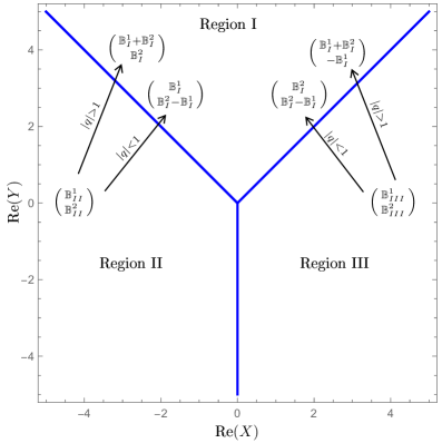
Figure 1: The three Stokes regions for $\mathbb{CP}^{1}$ at $\text{Im}(Y)=0$ and $\text{Im}(X)=-\frac{2\pi}{3}\cdot$ The analytic continuation of the blocks is shown from Regions II and III to Region I.

In what follows, we shall rederive all these results from a purely algebraic perspective.

3.1 Holomorphic blocks

We warm up by solving the LOIs in terms of $q$-hypergeometric functions in a region of parameter space that we will eventually identify as Region I in Figure 1. We shall focus first on the LOI (3.3) involving only $\widehat{p}_{y}$. This LOI is a second order $q$-difference equation so has two independent solutions. Also, since this LOI is insensitive to purely $x$-dependent factors, we can write each block $\mathbb{B}$ as follows:

$$\mathbb{B}(x,y;q)=f(x;q)\,g(x,y;q)\,,$$ (3.5)

where the function $f$ will be determined by solving the second LOI (3.4). We now define a new variable

$$t=\frac{y}{qx}\,\cdot$$ (3.6)

In terms of this variable, we have $\widehat{p}_{y}\equiv\sigma_{q}(y)=\sigma_{q}(t)$. The LOI (3.3) then takes the following form:

$$\big{[}\sigma_{q}(t)+(qx)^{-1}t^{-1}-x-x^{-1}+\sigma_{q}^{-1}(t)\big{]}g(x,t;q)=0\,.$$ (3.7)

In order to map this difference equation to the standard $q$-Goursat form, we define a new function $h$ as follows:

$$g(x,t;q) =\frac{\Theta_{q}(qxt)}{\Theta_{q}(qt)}\,h(x,t;q)\,.$$ (3.8)

The function $h$ satisfies an equation that can be cast in the $q$-Goursat form as follows:

$$\Big{[}tP_{1}\big{(}\sigma_{q}(t)\big{)}-Q_{1}\big{(}\sigma_{q}(t)\big{)}\Big{]}h(x,t;q)=0\,,$$ (3.9)

where the two $q$-difference operators $P_{1}$ and $Q_{1}$ are given by

$$P_{1}\big{(}\sigma_{q}(t)\big{)} =1\,;$$ (3.10)

$$Q_{1}\big{(}\sigma_{q}(t)\big{)} =\left(-\frac{\sigma_{q}(t)}{q}\right)^{-1}\big{(}1-\sigma_{q}(t)\big{)}\left(1-\frac{a}{q}\sigma_{q}(t)\right)\quad\text{ with }\quad a=qx^{2}\,.$$ (3.11)

3.1.1 First holomorphic block

One of the solutions to the equation (3.9) is given by the $q$-hypergeometric function ${}_{1}\phi_{1}$:

$$h_{1}(x,t;q)={}_{1}\phi_{1}\left(0;a;q,t^{-1}\right)={}_{1}\phi_{1}\left(0;qx^{2};q,qxy^{-1}\right).$$ (3.12)

The solution of the first LOI (3.3) can then be written as

$${\mathbb{B}}^{1}(x,y;q)=f_{1}(x;q)\frac{\Theta_{q}(qxt)}{\Theta_{q}(qt)}\,{}_{1}\phi_{1}(0;qx^{2};q,t^{-1})=f_{1}(x;q)\frac{\Theta_{q}(y)}{\Theta_{q}(x^{-1}y)}{}_{1}\phi_{1}(0;qx^{2};q,qxy^{-1})\,.$$ (3.13)

In order to solve for the block completely, we now fix $f_{1}(x;q)$ above by acting with the second LOI (3.4). The analysis is straightforward (but tedious) and we end up with the following $q$-difference equation for $f_{1}$:

$$f_{1}(qx;q)=\frac{q^{\frac{1}{2}}x}{(1-qx^{2})(1-q^{2}x^{2})}f_{1}(x;q)\,,$$ (3.14)

which is solved by

$$f_{1}(x)=\frac{(qx^{2},q;q)_{\infty}}{\Theta_{q}(-\sqrt{q}x)}\,\cdot$$ (3.15)

So, the holomorphic block is given by

$$\mathbb{B}^{1}(x,y;q) =\frac{(qx^{2},q;q)_{\infty}}{\Theta_{q}\left(-\sqrt{q}x\right)}\,\frac{\Theta_{q}(y)}{\Theta_{q}(x^{-1}y)}{}_{1}\phi_{1}(0;qx^{2};q,qxy^{-1})$$

$$=\frac{\Theta_{q}(y)}{\Theta_{q}\left(-\sqrt{q}x\right)\Theta_{q}(x^{-1}y)}\,{\mathcal{J}}(xy^{-1},x^{2};q)\,.$$ (3.16)

Here we have introduced the Hahn-Exton $q$-Bessel function denoted by ${\mathcal{J}}(x,y;q)$ and whose properties are given in the Appendix B. In principle, the holomorphic blocks can be multiplied by an elliptic factor $E(x,y;q)$ that satisfies $\widehat{p}_{x}E(x,y;q)=\widehat{p}_{y}E(x,y;q)=E(x,y;q)$, since the modified blocks would also satisfy the same LOIs. We have chosen the above block to match the result of Beem:2012mb .

3.1.2 Second holomorphic block

In order to find the second solution, we have to analyze the singularity structure of the $q$-difference equation (3.9) for $h(t)$, which can be written in the following form:

$$[a\,t\sigma_{q}^{-1}(t)+\big{(}1-(a+q)t\big{)}+qt\sigma_{q}(t)]h(t)=0\,.$$ (3.17)

We apply $\sigma_{q}(t)$ on the above equation and obtain the following second order equation:

$$\sigma_{q}^{2}(t)h(t)=-\left(q^{-2}t^{-1}(1-a\,qt-q^{2}t)\sigma_{q}(t)+q^{-1}a\right)h(t)\,.$$ (3.18)

Defining the two-component vector

$$\Phi(t)=\begin{pmatrix}h(t)\\ \sigma_{q}(t)h(t)\end{pmatrix},$$ (3.19)

the second order $q$-difference equation can be written as a matrix equation of the form:

$$\sigma_{q}(t)\Phi(t)=A(t)\Phi(t)\qquad\text{with}\qquad A(t)=\begin{pmatrix}0&1\\ -\mu(t)&\lambda(t)\end{pmatrix},$$ (3.20)

where

$$\mu(t)=\frac{a}{q}\quad\text{and}\quad\lambda(t)=\left(1+\frac{a}{q}-\frac{1}{q^{2}t}\right).$$ (3.21)

From the coefficient matrix $A(t)$ we see that $t\rightarrow\infty$ is a regular singular point and $t=0$ is an irregular singular point. We have already found one of the regular solutions near $t=\infty$ in (3.12). In order to find the other holomorphic solution near $t=\infty$, let us write the coefficient matrix near infinity:

$$A(\infty)=\begin{pmatrix}0&1\\ -\frac{a}{q}&1+\frac{a}{q}\end{pmatrix}.$$ (3.22)

The eigenvalues of this matrix are $\{1,\frac{a}{q}\}$. We will restrict ourselves to the non-resonant case in which $a\neq q$ (which is equivalent to the condition $x\neq\pm 1$). The procedure to obtain the second solution is now standard (see TAB for a review). First we write the character matrix

$$\chi_{\infty}(t)=\begin{pmatrix}1&0\\ 0&e_{\frac{a}{q}}(t)\end{pmatrix},\quad\text{ where }\quad e_{\omega}(t)=\frac{\Theta_{q}(t)}{\Theta_{q}({\omega}t)}\,\cdot$$ (3.23)

For the case ${\omega}=\frac{a}{q}$, one can simplify this and rewrite it as

$$e_{\frac{a}{q}}(t)=\frac{q}{a}\,\frac{\Theta_{q}(qt)}{\Theta_{q}(at)}\,\cdot$$ (3.24)

The second solution is then written as

$$h_{2}(t)=e_{\frac{a}{q}}(t)\,\ell_{2}(t)\,,$$ (3.25)

where $\ell_{2}$ can be obtained by solving the matrix eigenvalue equation:

$$\begin{pmatrix}\ell_{1}(qt)&\ell_{2}(qt)\\ \ell_{3}(qt)&\ell_{4}(qt)\end{pmatrix}\cdot\begin{pmatrix}1&0\\ 0&\frac{a}{q}\end{pmatrix}=\begin{pmatrix}0&1\\ -\mu(t)&\lambda(t)\end{pmatrix}\cdot\begin{pmatrix}\ell_{1}(t)&\ell_{2}(t)\\ \ell_{3}(t)&\ell_{4}(t)\end{pmatrix}.$$ (3.26)

If we set $\ell_{1}(t)\equiv h_{1}(t)$, we find that $\ell_{2}(t)$ satisfies the following second order $q$-difference equation:

$$\left(\sigma_{q}^{2}(t)-\frac{q}{a}\lambda(t)\sigma_{q}(t)+\frac{q^{2}}{a^{2}}\mu(t)\right)\ell_{2}(t)=0\,.$$ (3.27)

One can map this to the standard $q$-Goursat form by the change of variables:

$$\widetilde{t}=\frac{a}{q}t\,,\qquad\widetilde{a}=\frac{q^{2}}{a}\,\cdot$$ (3.28)

The second solution $h_{2}(t)$ can then be written (up to constant prefactors) as

$$h_{2}(t)=\frac{\Theta_{q}(qt)}{\Theta_{q}(at)}\,{}_{1}\phi_{1}\left(0;\frac{q^{2}}{a};q,\frac{q}{at}\right).$$ (3.29)

The relation between $g_{2}$ (which solves (3.7)) and $h_{2}$ is the same as in equation (3.8). So all that remains to obtain the second independent holomorphic block is to fix the prefactor $f_{2}$ in (3.5). This can be done by using the second LOI; the analysis is similar to what was done for the first block and we simply present the final result (up to elliptic factors):

$$\mathbb{B}^{2}(x,y;q) =\frac{(qx^{-2},q;q)_{\infty}\,\Theta_{q}(y)}{\Theta_{q}(-\sqrt{q}x)\,\Theta_{q}(xy)}\,{}_{1}\phi_{1}(0;qx^{-2};q,qx^{-1}y^{-1})$$

$$=\frac{\Theta_{q}(y)}{\Theta_{q}(-\sqrt{q}x)\,\Theta_{q}(xy)}\,{\mathcal{J}}(x^{-1}y^{-1},x^{-2};q)\,.$$ (3.30)

3.1.3 Finding a region in parameter space

Given the explicit expression for the blocks in terms of the ${\mathcal{J}}$-functions, one can make use of the series expansion in (B.8) to understand the region of validity of these expressions for the blocks in either $q$-chamber. Essentially the convergence of the expansion requires that for ${\mathcal{J}}(x,y;q)$, we have $|x|<1$. For the holomorphic blocks in (3.16) and (3.30), we obtain:

$$\text{Re}(Y)-\text{Re}(X)>0\qquad\text{and}\qquad\text{Re}(Y)+\text{Re}(X)>0\,.$$ (3.31)

This precisely maps to Region I in Figure 1 and we infer that the blocks we have constructed are a basis of solutions to the LOIs in Region I. Henceforth, we shall denote these blocks as $(\mathbb{B}^{1}_{I},\mathbb{B}^{2}_{I})$. It is important to note here that the blocks we have obtained in Region I in terms of $q$-hypergeometric functions are valid expressions independent of whether $|q|<1$ or $|q|>1$, since the method of solving the $q$-difference equations made no assumptions regarding the $q$-chamber.

4 Stokes phenomena for $\bm{\mathbb{CP}^{1}}$ blocks

The holomorphic blocks we solved for in Region I are solutions to two $q$-difference equations. Apart from meromorphic factors, the non-trivial part is the $q$-hypergeometric function ${}_{1}\phi_{1}$ with vanishing first argument. Both of these solutions are analytic near $t=\infty$. In this section, we compute non-trivial solutions of the $q$-difference equation satisfied by ${}_{1}\phi_{1}$ but near the irregular singular point $t=0$ using the $q$-Borel and the $q$-Laplace transformations discussed in Section 2.

In particular, we derive in detail the connection formulae that relate the solutions near the irregular singular point $t=0$ to those we obtained near $t=\infty$. Our claim is that these connection formulae fully encode and explain the Stokes phenomena observed for the holomorphic blocks, which were derived using the block-integral representation in Beem:2012mb . More importantly as we show, the same connection formula can contain information about the analytic continuation to multiple regions in parameter space for the $\mathbb{CP}^{1}$ model.

We start with the equation (3.17):

$$\left[at\sigma_{q}^{-1}(t)+(1-(a+q)t)+qt\sigma_{q}(t)\right]h(t)=0\,.$$ (4.1)

We look for solutions around $t=0$, and we assume the following ansatz for the two linearly independent solutions RSZ ; OHY :

$$h_{1}(t) =\frac{1}{\Theta_{q}(aqt)}\,u_{1}(t)\,,$$ (4.2)

$$h_{2}(t) =\Theta_{q}(qt)\,u_{2}(t)\,.$$ (4.3)

The $q$-Borel resummation, as we shall see, will be done on the $u_{k}(t)$ part of the solution. We shall deal with each of these solutions in turn, and we will see that the way $q$-Borel resummation is carried out on the solution depends crucially on the chamber, i.e., whether $|q|<1$ or $|q|>1$.

4.1 Connection formulae for the first solution

We begin with $h_{1}(t)$ and given the ansatz in (4.2), $u_{1}(t)$ satisfies the following equation

$$\left[-aq^{2}t^{2}\sigma_{q}(t)+(1-(a+q)t)-\sigma_{q}^{-1}(t)\right]u_{1}(t)=0\,.$$ (4.4)

This can be solved by a power series solution of the form $u_{1}(t)=\sum_{m\geq 0}a_{m}t^{m}$. Taking the $q$-Borel transform of this equation by ${\mathcal{B}}_{q}^{-}$ we find

$$\left[aq^{3}\tau^{2}+(aq+q^{2})\tau+1-\sigma_{q}(\tau)\right]\mathcal{B}_{q}^{-}[u_{1}](\tau)=0\,,$$ (4.5)

which is solved by

$$\mathcal{B}_{q}^{-}[u_{1}](\tau)=\frac{1}{(-q^{2}\tau,-aq\tau;q)_{\infty}}\,\cdot$$ (4.6)

4.1.1 The $\bm{|q|<1}$ chamber

The $q$-Laplace transform for $|q|<1$ is given by

$$\mathcal{L}_{q}^{-}\left[\mathcal{B}_{q}^{-}[u_{1}](\tau)\right](t)=\frac{1}{2\pi i}\oint_{\Gamma_{\epsilon}}\frac{d\tau}{\tau}\frac{\Theta_{q}\left(-t\tau^{-1}\right)}{(-q^{2}\tau,-aq\tau;q)_{\infty}}\,\cdot$$ (4.7)

This integral can be done by deforming the contour and summing up the contributions from the simple poles of $\mathcal{B}_{q}^{-}[u_{1}](\tau)$ for $|q|<1$ along with a possible contribution from $\tau=\infty$. We restrict the calculation to this $q$-chamber because the theta function does not contribute to poles. As shown in Morita:2011hx ; OHY , the contribution from infinity vanishes for this integral and so the $q$-Laplace transform reduces to minus the sum over the poles of the $q$-Pochhammers in (4.7).

There are two different sets of poles which are located at

$$\tau^{(1)}_{r}=-q^{-(r+2)}\quad\text{ and }\quad\tau^{(2)}_{r}=-a^{-1}q^{-(r+1)}\qquad\text{ for }r=0,1,\cdots\,.$$ (4.8)

The residue for the first set of poles $\tau^{(1)}_{r}$ is given by

$$-\text{Res}_{\tau^{(1)}_{r}}=\frac{\Theta_{q}(q^{2}t)}{\left(\frac{a}{q},q;q\right)_{\infty}}\frac{(-1)^{r}q^{\frac{r}{2}(r-1)}}{\left(\frac{q^{2}}{a},q;q\right)_{r}}\left(\frac{q}{at}\right)^{r}.$$ (4.9)

Denoting the sum over this first set of residues to be $I_{1}$, we obtain

$$I_{1}=\frac{\Theta_{q}(q^{2}t)}{\left(\frac{a}{q},q;q\right)_{\infty}}{}_{1}\phi_{1}\left(0;\frac{q^{2}}{a};q,\frac{q}{at}\right).$$ (4.10)

Similarly, the residue from the other set of poles $\tau^{(2)}_{r}$ is given by

$$-\text{Res}_{\tau^{(1)}_{r}}=\frac{\Theta_{q}(aqt)}{\left(a,q;q\right)_{\infty}}\frac{(-1)^{r}q^{\frac{r}{2}(r-1)}}{\left(a,q;q\right)_{r}}\left(\frac{1}{t}\right)^{r}.$$ (4.11)

Denoting the sum over the second set of residues to be $I_{2}$, we obtain

$$I_{2}=\frac{\Theta_{q}(aqt)}{\left(\frac{q}{a},q;q\right)_{\infty}}{}_{1}\phi_{1}\left(0;a;q,\frac{1}{t}\right).$$ (4.12)

Thus, the connection formula in the $|q|<1$ chamber is given by

$$h_{1}(t) \longrightarrow\frac{1}{(qa^{-1},q;q)_{\infty}}{}_{1}\phi_{1}\left(0;a;q,\frac{1}{t}\right)+\frac{1}{(aq^{-1},q;q)_{\infty}}\frac{\Theta_{q}(q^{2}t)}{\Theta_{q}(aqt)}{}_{1}\phi_{1}\left(0;\frac{q^{2}}{a};q,\frac{q}{at}\right)$$

$$\longrightarrow\frac{1}{\Theta_{q}(a)}\mathcal{J}\left(q^{-1}t^{-1},q^{-1}a;q\right)+\frac{\Theta_{q}(q^{2}t)}{\Theta_{q}(aq^{-1})\Theta_{q}(aqt)}\mathcal{J}\left(a^{-1}t^{-1},qa^{-1};q\right).$$ (4.13)

Here we have multiplied the $q$-Borel-resummed functions by the $\Theta_{q}$ prefactor in (4.2). We recognize the $q$-hypergeometric functions to be precisely those that appear in the holomorphic blocks in Region I. We now multiply the r.h.s by the following prefactor in order to obtain the holomorphic blocks of the $\mathbb{CP}^{1}$ theory:

$$\Omega_{1}(x,y;q)=-\frac{\Theta_{q}(qx^{2})\Theta_{q}(y)}{\Theta_{q}(-\sqrt{q}x)\Theta_{q}(x^{-1}y)}\,\cdot$$ (4.14)

This factor is nothing but $f(x;q)\frac{\Theta_{q}(qxt)}{\Theta_{q}(qt)}$ arising due to (3.5) and (3.8) and is essential for the block to satisfy both the LOIs of $\mathbb{CP}^{1}$. By substituting $t^{-1}=qxy^{-1}$ and $a=qx^{2}$ in (4.13) and after some algebraic manipulations we find the following connection formula:

$$\Omega_{1}h_{1} \longrightarrow\mathbb{B}^{2}_{I}-\mathbb{B}^{1}_{I}\,.$$ (4.15)

The above connection formula holds for $|q|<1$. The function appearing on the l.h.s. will eventually be identified with the holomorphic block in a Stokes region distinct from the Region I we have already encountered; but in order to complete the identification, we also need to find the connection formula in the $|q|>1$ chamber.

4.1.2 The $\bm{|q|>1}$ chamber

For $|q|>1$, the $q$-Laplace transform ${\mathcal{L}}^{-}_{q,\lambda}$ fails to lead to a convergent integral. A similar problem for ${\mathcal{L}}^{+}_{q,\lambda}$ is encountered in the $|q|<1$ chamber in OHY . The method proposed to deal with this issue was to introduce $p=\sqrt{q}$ and to perform the $p$-Borel transform followed by a $p$-Laplace transform. We have suitably adapted their methods for the $|q|>1$ case and have obtained the following connection formula (with $q=p^{2}$):

$$h_{1}(t)\longrightarrow\psi_{1}(t,p,\lambda)\,\mathcal{J}\left(a^{-1}t^{-1},qa^{-1};q\right)+\psi_{2}(t,p,\lambda)\,\mathcal{J}(q^{-1}t^{-1},q^{-1}a;q)\,,$$ (4.16)

where the coefficients $\psi_{i}$ are given by

$$\psi_{1}(t,p,\lambda) =\frac{\Theta_{q}(apq^{2}\lambda^{2})\Theta_{q}(-p\lambda t^{-1})\Theta_{q}(-q\lambda t^{-1})}{\Theta_{q}(aqt)\Theta_{q}(-ap\lambda)\Theta_{q}(-ap^{2}\lambda)\Theta_{q}(\lambda^{2}p^{5}t^{-1})}\,,$$ (4.17)

$$\psi_{2}(t,p,\lambda) =\frac{\Theta_{q}(a^{-1}p^{-3}\lambda^{-2})\Theta_{q}(-p\lambda t^{-1})\Theta_{q}(-q\lambda t^{-1})}{\Theta_{q}(aqt)\Theta_{q}(-q^{-1}\lambda^{-1})\Theta_{q}(-p^{-1}\lambda^{-1})\Theta_{q}(apq\lambda^{2}t^{-1})}\,\cdot$$ (4.18)

This is the main new result of this work and it is proved in detail in Appendix C. According to OHY ; DRELO and as discussed in subsection 2.2, $\lambda$ is such that $\left[\lambda\right]\in\left(\mathbb{C}^{\star}/q^{\mathbb{Z}}\right)\setminus\{\left[1\right]\}$. We now claim that the holomorphic blocks (built on the $h_{1}(t)$) satisfy both the LOIs of $\mathbb{CP}^{1}$ model only for two values of $\lambda$. Furthermore, we find that precisely for these values, the connection formula in (4.16) coincides with those derived in Beem:2012mb by using the block-integral representation. Let us see this in detail.

1. We set $\lambda=-p^{-1}=-q^{-\frac{1}{2}}$ and substitute $t=\frac{y}{qx}$ and $a=qx^{2}$. The coefficients $\psi_{i}$ then take the following simplified values:

   $$\psi_{1}=-\frac{\Theta_{q}(x^{-1}y)}{\Theta_{q}(qx^{2})\Theta_{q}(xy)}\,;\qquad\psi_{2}=0\,.$$ (4.19)

   The vanishing of $\psi_{2}$ is due to the factor $\Theta_{q}(-p^{-1}\lambda^{-1})$ in the denominator, which tends to infinity for the choice of $\lambda=-p^{-1}$. The connection formula therefore simplifies to the following form:

   $$h_{1}(t)\longrightarrow-\frac{\Theta_{q}(x^{-1}y)}{\Theta_{q}(qx^{2})\Theta_{q}(xy)}\mathcal{J}(x^{-1}y^{-1},x^{-2};q)\,.$$ (4.20)

   Now to obtain the holomorphic block of the $\mathbb{CP}^{1}$ theory we multiply with the same factor $\Omega_{1}$ as in (4.14). We thereby obtain the following connection formula for the solution around $t=0$ for this particular value of $\lambda$:

   $$\Omega_{1}h_{1}\longrightarrow \;\frac{\Theta_{q}(y)}{\Theta_{q}(-\sqrt{q}x)\Theta_{q}(xy)}\mathcal{J}(x^{-1}y^{-1},x^{-2};q)$$

   $$= \;\mathbb{B}^{2}_{I}\,.$$ (4.21)

2. We set $\lambda=-pa^{-1}=-q^{-\frac{1}{2}}x^{-2}$ and the coefficients $\psi_{i}$ take the following values:

   $$\psi_{1}=0\,;\qquad\psi_{2}=\frac{1}{\Theta_{q}(qx^{2})}\,\cdot$$ (4.22)

   The vanishing of $\psi_{1}$ is because $\Theta_{q}(-ap\lambda)$ tends to infinity for $\lambda=-q^{-\frac{1}{2}}x^{-2}$. Using the same multiplicative factor $\Omega_{1}$ to satisfy the LOIs of the $\mathbb{CP}^{1}$ theory we obtain the analytically continued solution:

   $$\Omega_{1}h_{1}\longrightarrow -\frac{\Theta_{q}(y)}{\Theta_{q}(-\sqrt{q}x)\Theta_{q}(x^{-1}y)}\mathcal{J}(xy^{-1},x^{2};q)$$

   $$= -\mathbb{B}^{1}_{I}\,.$$ (4.23)

We summarize the results of this subsection in Figure 2.

Figure 2: Summary of the connection formula for the solution $\Omega_{1}h_{1}$. All connection formulae are obtained by first using the ${\mathcal{B}}^{-}$ Borel transform, followed by the inverse Laplace transform ${\mathcal{L}}^{-}$. For $|q|<1$ there is a unique way to analytically continue the solution. For $|q|>1$, there are two ways to analytically continue the solution consistent with both LOIs of the $\mathbb{CP}^{1}$ theory, as shown.

4.2 Connection formulae for the second solution

We now turn to the second solution $h_{2}(t)=\Theta_{q}(qt)u_{2}(t)$. The $q$-difference equation satisfied by $u_{2}(t)$ is given by

$$\left[-\sigma_{q}(t)+(1-(a+q)t)-a\,t^{2}\,\sigma_{q}^{-1}(t)\right]u_{2}(t)=0\,.$$ (4.24)

We act with the $q$-Borel transform ${\mathcal{B}}^{+}_{q}$ on the above equation and using the identities in (2.3), one can check that the $q$-Borel transformed solution satisfies the following equation:

$$\sigma_{q}(\tau)\mathcal{B}_{q}^{+}[u_{2}](\tau)=\frac{1}{(a\tau+1)(q\tau+1)}\mathcal{B}_{q}^{+}[u_{2}](\tau)\,,$$ (4.25)

which is solved by

$$\mathcal{B}_{q}^{+}[u_{2}](\tau)=\left(-a\tau,-q\tau;q\right)_{\infty}\,.$$ (4.26)

4.2.1 The $\bm{|q|>1}$ chamber

For $|q|>1$, the $q$-Pochhammer has simple poles and as we did for the previous solution, it is possible to use the $q$-Laplace transform ${\mathcal{L}}_{q}^{+}$ in equation (2.18) to obtain the $q$-Borel resummed solution:

$$\mathcal{L}_{q}^{+}\left[\mathcal{B}_{q}^{+}[u_{2}](\tau)\right](t)=\frac{1}{2\pi i}\oint_{\Gamma_{\epsilon}}\frac{d\tau}{\tau}\left(-a\tau,-q\tau;q\right)_{\infty}\Theta_{q}^{-1}\left(-qt\tau^{-1}\right),$$ (4.27)

where $\Gamma_{\epsilon}$ is a contour that encircles the origin. There are two infinite sets of poles, located at

$$\tau^{(1)}_{r}=-a^{-1}q^{r+1}\quad\text{ and }\quad\tau^{(2)}_{r}=-q^{r}\qquad\text{ for }r=0,1,\cdots\,.$$ (4.28)

Then the residue for the first set of poles $\tau^{(1)}_{r}$ is given by

$$-\text{Res}_{\tau^{(1)}_{r}}=\frac{(q^{2}a^{-1};q)_{\infty}(q^{-1};q^{-1})_{\infty}}{\Theta_{q}(ta)}\frac{(-1)^{r}q^{\frac{r}{2}(r-1)}(qt^{-1}a^{-1})^{r}}{(q^{2}a^{-1},q;q)_{r}}\,\cdot$$ (4.29)

Then we can analytically do the complex integral for $|q|>1$ by summing up all the residues for $r\in[0,\infty]$, which gives

$$I_{1}=\frac{(q^{2}a^{-1};q)_{\infty}(q^{-1};q^{-1})_{\infty}}{\Theta_{q}(ta)}~{}{}_{1}\phi_{1}(0;q^{2}a^{-1};q,qt^{-1}a^{-1})\,.$$ (4.30)

The sign is reversed due to the fact that we have to consider minus the sum of residues at the poles $\tau^{(1)}_{r}$. Similarly, the residues arising from the second set of poles $\tau^{(2)}_{r}$ are given by

$$-\text{Res}_{\tau^{(2)}_{r}}=\frac{(a;q)_{\infty}(q^{-1};q^{-1})_{\infty}}{\Theta_{q}(qt)}\frac{(-1)^{n}q^{\frac{n}{2}(n-1)}t^{-n}}{(a,q;q)_{n}}\,\cdot$$ (4.31)

Summing over all residues, we obtain

$$I_{2}=\frac{(a;q)_{\infty}(q^{-1};q^{-1})_{\infty}}{\Theta_{q}(qt)}~{}{}_{1}\phi_{1}(0;a;q,t^{-1})\,.$$ (4.32)

It is interesting to observe that we obtain the same $q$-hypergeometric series as we did in $|q|<1$ chamber. Putting together the two contributions $I_{1}$ and $I_{2}$, and rewriting the $q$-hypergeometric functions in terms of the ${\mathcal{J}}$-function, we obtain the connection formula for $|q|>1$:

$$h_{2}(t)\longrightarrow(q^{-1};q^{-1})_{\infty}\left[\mathcal{J}(q^{-1}t^{-1},q^{-1}a;q)+\frac{\Theta_{q}(qt)}{\Theta_{q}(at)}\mathcal{J}(t^{-1}a^{-1},qa^{-1};q)\right].$$ (4.33)

Now to apply this connection formula to the blocks in the $\mathbb{CP}^{1}$ case we have to multiply by the following prefactor (which follows from an analysis similar to the one that led to $\Omega_{1}$):

$$\Omega_{2}(x,y;q)=\frac{\Theta_{q}(y)}{\Theta_{q}(-\sqrt{q}x)\Theta_{q}(x^{-1}y)}\,\cdot$$ (4.34)

By setting $t^{-1}=qxy^{-1}$ and $a=qx^{2}$, and identifying the terms on the r.h.s of the connection formula in (4.33) with the holomorphic blocks in Region I of the $\mathbb{CP}^{1}$ theory, we obtain the following connection formula for $|q|>1$:

$$\Omega_{2}h_{2}\longrightarrow\mathbb{B}^{1}_{I}+\mathbb{B}^{2}_{I}\,.$$ (4.35)

4.2.2 The $\bm{|q|<1}$ chamber

The connection formula for this case has been derived in OHY and we simply present the result relating the solution near $t=0$ to the regular solutions near $t=\infty$:

$$h_{2}(t)\longrightarrow\chi_{1}(t,p,\lambda)~{}\mathcal{J}\left(q^{-1}t^{-1},q^{-1}a;q\right)+\chi_{2}(t,p,\lambda)~{}\mathcal{J}\left(a^{-1}t^{-1},qa^{-1};q\right),$$ (4.36)

where the coefficients $\chi_{i}$ are given by

$$\chi_{1}(t,p,\lambda) =\frac{\Theta_{q}(qt)\Theta_{q}(-a\lambda)\Theta_{q}(-a\lambda p)\Theta_{q}\left(pt\lambda^{-2}\right)}{\Theta_{q}(ap\lambda^{2})\Theta_{q}\left(-pt\lambda^{-1}\right)\Theta_{q}\left(-qt\lambda^{-1}\right)\Theta_{q}(qa^{-1})}\,,$$ (4.37)

$$\chi_{2}(t,p,\lambda) =\frac{\Theta_{q}(qt)\Theta_{q}(-q\lambda)\Theta_{q}(-pq\lambda)\Theta_{q}\left(pqta^{-1}\lambda^{-2}\right)}{\Theta_{q}\left(-pt\lambda^{-1}\right)\Theta_{q}\left(-qt\lambda^{-1}\right)\Theta_{q}(ap\lambda^{2})\Theta_{q}(aq^{-1})}\,\cdot$$ (4.38)

As for the case studied previously, the connection formula involves the parameter $\lambda$ and we choose the same two values as before. Exactly for these values, it turns out that these provide solutions to both the LOIs of the $\mathbb{CP}^{1}$ theory.

1. We choose the parameter $\lambda=-p^{-1}=-q^{-\frac{1}{2}}$, for which the coefficients become

   $$\chi_{1}=\frac{\Theta_{q}(a)}{\Theta_{q}\left(qa^{-1}\right)}=1\,;\qquad\chi_{2}=0\,.$$ (4.39)

   The last equality is due to the factor $\Theta_{q}(-pq\lambda)=\Theta_{q}(q)$, which vanishes. To satisfy both the LOIs, we have to multiply the above with the same prefactor $\Omega_{2}$ given in (4.34). Substituting $t=\frac{y}{qx}$ and $a=qx^{2}$ we obtain the following connection formula in terms of the holomorphic blocks:

   $$\Omega_{2}h_{2}\longrightarrow \;\frac{\Theta_{q}(y)}{\Theta_{q}(-\sqrt{q}x)\Theta_{q}(x^{-1}y)}\mathcal{J}(xy^{-1},x^{2};q)$$

   $$= \;\mathbb{B}^{1}_{I}\,.$$ (4.40)

2. The second consistent choice of $\lambda$ is given by $\lambda=-pa^{-1}=-q^{-\frac{1}{2}}x^{-2}$. Due to the vanishing factor $\Theta_{q}(-a\lambda p)=\Theta_{q}(p^{2})=0$, we find that

   $$\chi_{1}=0\,;\qquad\chi_{2}=\frac{\Theta_{q}(x^{-1}y)\Theta_{q}(qx^{-2})}{\Theta_{q}(xy)\Theta_{q}\left(x^{2}\right)}\,\cdot$$ (4.41)

   The connection formula in terms of blocks then reads:

   $$\Omega_{2}h_{2}\longrightarrow \;\frac{\Theta_{q}(y)}{\Theta_{q}(-\sqrt{q}x)\Theta_{q}(xy)}\mathcal{J}(x^{-1}y^{-1},x^{-2};q)$$

   $$= \;\mathbb{B}_{I}^{2}\,.$$ (4.42)

We summarize the results of this subsection in Figure 3.

Figure 3: Summary of the connection formula for the solution $\Omega_{2}h_{2}$. All connection formulae are obtained by first using the ${\mathcal{B}}^{+}$ Borel transform, followed by the inverse Laplace transform ${\mathcal{L}}^{+}$. For $|q|>1$ there is a unique way to analytically continue the solution. For $|q|<1$, there are two ways to analytically continue the solution consistent with both LOIs of the $\mathbb{CP}^{1}$ theory, as shown.

5 Concluding remarks

We have focussed on holomorphic blocks of the $\mathbb{CP}^{1}$ model. Semi-classically, the theory has two massive vacua and from the general analysis of Beem:2012mb , it follows that there are two holomorphic blocks in any given region of parameter space labelled by the complexified twisted mass and FI parameter $(X,Y)$, respectively. The blocks, in turn, are solutions to two linear second order $q$-difference equations. In one region of parameter space, we could easily solve both the LOIs in terms of the $q$-hypergeometric function ${}_{1}\phi_{1}$ as the first LOI (3.3) has a regular singular point. We denoted these blocks by $(\mathbb{B}_{I}^{1},\mathbb{B}_{I}^{2})$.

Obtaining the solutions in the other regions of parameter space turned out to be more subtle because these correspond to the solutions of first LOI (3.3) near an irregular singular point. In the nomenclature of OHY (see also the talk OHYtalk where more details are given), in each chamber (either $|q|<1$ or $|q|>1$), one of the solutions is a convergent series while the other is a divergent series. For the convergent series there is a unique way to analytically continue the solution while the analytic continuation of the divergent series depends on a complex parameter $\lambda$. In other words, for a given $q$-divergence series, the Stokes region depends on $\lambda$ OHYtalk .

Taking into account the second LOI (3.4) satisfied by the holomorphic blocks of the $\mathbb{CP}^{1}$ theory, it turned out that only for two values of $\lambda$ did the analytic continuation lead to consistent holomorphic blocks. Putting these different mathematical notions together, one expects three Stokes regions in the $\mathbb{CP}^{1}$ theory, which agrees with what was found in Beem:2012mb . In order to make more precise comparisons with their results, let us rearrange the connection formulae summarized in Figure 2 and Figure 3 such that we pair the blocks together for a given value of $\lambda$, as shown in Figure 4. We observe that we exactly reproduce the results of Beem:2012mb shown in Figure 1 by noting that the right half of Figure 4 corresponds to analytic continuation of blocks from Region II and the left half to that from Region III. It is thus the choice of $\lambda$ that effectively distinguishes the Stokes regions.

Figure 4: Analytic continuation of the blocks for $\lambda=-q^{-\frac{1}{2}}$ and $\lambda=-q^{-\frac{1}{2}}x^{-2}$.

It now remains to identify the precise expressions for the blocks in the different Stokes regions. While the path to do this has already been outlined in Beem:2012mb we now comment on how the algebraic approach adds to the discussion. The basic idea in Beem:2012mb is to exploit the fact that while the holomorphic blocks have different analytic behaviour in the $|q|<1$ and $|q|>1$ chambers, they have identical series expansions. So, if one is able to find an expression for the block in a given chamber as a single ${\mathcal{J}}$-function, the $q$-expansion in the other chamber is guaranteed to be the same. However, given such a form for the block in one chamber, the algebraic approach guarantees that it will have the correct analytic continuation in the other chamber.

We begin with the $\lambda=-q^{-\frac{1}{2}}$ case and consider the analytic continuation results for $\Omega_{2}h_{2}$ in $|q|<1$ chamber and $\Omega_{1}h_{1}$ in $|q|>1$ chamber (right half of Figure 4). We see that these coincide with individual blocks valid in the Region I as derived in subsection 3.1. Following Beem:2012mb we use the identities (B.10) and (B.11) valid in the respective $q$-chambers to rewrite the $\mathcal{J}$-functions and claim that the pair of blocks for $\lambda=-q^{-\frac{1}{2}}$ is given by

$$\mathbb{B}_{R_{1}}:=\Big{(}\Omega_{2}h_{2}\Big{)}_{\lambda=-q^{-\frac{1}{2}}} =\frac{\Theta_{q}(y)}{\Theta_{q}(-\sqrt{q}x)\Theta_{q}(x^{-1}y)}\mathcal{J}(x^{2},xy^{-1};q)\,.$$ (5.1)

$$\mathbb{B}_{R_{2}}:=\Big{(}\Omega_{1}h_{1}\Big{)}_{\lambda=-q^{-\frac{1}{2}}} =-\frac{\Theta_{q}(y)\Theta_{q}(qx^{2})}{\Theta_{q}(-\sqrt{q}x)\Theta_{q}(qxy)\Theta_{q}(x^{-1}y)}\mathcal{J}(xy,x^{-1}y;q)\,.$$ (5.2)

Note that we have used an identity valid only in one $q$-chamber and not the other to write the above expressions. In Beem:2012mb a formula for the ${\mathcal{J}}$-function was conjectured in order to make sense of the connection formula in the other chamber. From the perspective of blocks as contour integrals, it is not obvious why these ${\mathcal{J}}$-functions can be continued to give the results in the other $q$-chamber. However, from the explicit analytic continuation of the $\Omega_{i}h_{i}$ for this value of $\lambda$ derived in the previous section, it is guaranteed and can be taken as a proof of that conjectured formula.

A similar analysis can be done for the other value of $\lambda=-q^{-\frac{1}{2}}x^{-2}$ by making use of the same identities (B.10) and (B.11) but focussing on the left half of Figure 4:

$$\mathbb{B}_{R_{3}} :=\Big{(}\Omega_{2}h_{2}\Big{)}_{\lambda=-q^{-\frac{1}{2}}x^{-2}}=\frac{\Theta_{q}(y)}{\Theta_{q}(-\sqrt{q}x)\Theta_{q}(xy)}\mathcal{J}(x^{-2},x^{-1}y^{-1};q)\,.$$ (5.3)

$$\mathbb{B}_{R_{4}} :=\Big{(}\Omega_{1}h_{1}\Big{)}_{\lambda=-q^{-\frac{1}{2}}x^{-2}}=\frac{\Theta_{q}(y)\Theta_{q}(x^{2})}{\Theta_{q}(-\sqrt{q}x)\Theta_{q}(xy)\Theta_{q}(xy^{-1})}\mathcal{J}(x^{-1}y,xy;q)\,.$$ (5.4)

We now claim that the constraints arising from the convergence of the power series expansions of these new ${\mathcal{J}}$-functions should lead to new Stokes regions, where these blocks form a well-defined basis. Furthermore, we will show that the pairing based on the choice of $\lambda$ suggested above and the convergence properties are consistent because the domains of validity of the three pairs of blocks allow a single covering of the parameter space. The parameter space that is under consideration is spanned by $X$ and $Y$ defined in (3.1). The blocks are written in terms of the $\mathcal{J}$-functions up to rational products of theta factors. Each $\mathcal{J}(x,y;q)$ function is defined in the $|x|<1$ region. The region in which a pair of blocks is defined, is determined by the overlap of the domains of validity of the two $\mathcal{J}$-functions associated to that pair of blocks. We work these regions out in detail now.

For the original pair of blocks, namely $\mathbb{B}^{1}_{I}$ and $\mathbb{B}^{2}_{I}$, this was already done in the subsection 3.1.3 and the region where both the blocks are defined is given by the overlap of

$$\text{Re}(X)-\text{Re}(Y)<0\quad\text{ and }\quad\text{Re}(X)+\text{Re}(Y)>0\,.$$ (5.5)

This overlap region, which we call Region I, is a right-angled wedge in the upper half of $\text{Re}(X,Y)$-plane. Let us apply the same idea to the other two pairs of blocks. The pair of blocks ($\mathbb{B}_{R_{1}}$, $\mathbb{B}_{R_{2}}$) are defined in the region bounded by

$$\text{Re}(X)<0\quad\text{ and }\quad\text{Re}(X)+\text{Re}(Y)<0\,.$$ (5.6)

This region (Region II) is bounded by the negative $\text{Re}(Y)$-axis and the $\text{Re}(X)+\text{Re}(Y)=0$ line in the upper half of $\text{Re}(X,Y)$-plane. Notice the latter boundary matches with the second boundary ($\text{Re}(X)+\text{Re}(Y)=0$) of the Region I. Finally, the pair of blocks ($\mathbb{B}_{R_{3}}$, $\mathbb{B}_{R_{4}}$) are defined in the region (Region III) bounded by

$$\text{Re}(X)>0\quad\text{ and }\quad\text{Re}(X)-\text{Re}(Y)>0\,.$$ (5.7)

It is easy to see that Region III is bounded by the negative $\text{Re}(Y)$-axis and the line $\text{Re}(X)-\text{Re}(Y)=0$ in the upper half of $\text{Re}(X,Y)$-plane. The former boundary matches with the first boundary ($\text{Re}(X)=0$) of the Region II and the latter boundary matches with the first boundary ($\text{Re}(X)-\text{Re}(Y)=0$) of the Region I. This completes the (re)derivation of the Stokes regions in the $\mathbb{CP}^{1}$ model and we summarize this discussion in the Figure 5.

Figure 5: Thick (blue) lines are the Stokes lines dividing the $\text{Re}(X,Y)$-plane into three Stokes regions. The domain of validity of each block is shown by arrows. The basis of blocks in each Stokes region is given by the two blocks in larger font. (Dotted lines play no role in defining the Stokes regions.)

It is useful to recall that in Beem:2012mb these Stokes regions were obtained by using various means including the self-mirror property of the $\mathbb{CP}^{1}$ model. In the algebraic approach, we did not use such physical considerations and focused solely on the LOIs and the analytic continuation of the $q$-hypergeometric functions. It would be interesting to see if this approach can be generalized to other models with irregular singular points for the blocks such as the $\mathbb{CP}^{N}$ models where the block-integrals and contour deformation methods might be more difficult to implement.

Appendix A The $\bm{q}$-Goursat equation

The $q$-analogue of Goursat’s equation is given as follows (we follow the conventions in OHYtalk ; Adachi ):

$$[xP_{r}\big{(}\sigma_{q}(x)\big{)}-Q_{s}\big{(}\sigma_{q}(x)\big{)}]f(x)=0\,,$$ (A.1)

where the two polynomial $q$-difference operators are given by

$$P_{r}\big{(}\sigma_{q}(x)\big{)}=\big{(}-\sigma_{q}(x)\big{)}^{\mu}\prod_{j=1}^{r}\big{(}1-a_{j}\sigma_{q}(x)\big{)}\,;$$ (A.2)

$$Q_{s}\big{(}\sigma_{q}(x)\big{)}=\left(-\frac{\sigma_{q}(x)}{q}\right)^{m}\prod_{k=0}^{s}\left(1-\frac{b_{k}}{q}\sigma_{q}(x)\right).$$ (A.3)

Here $b_{0}=q$ and $m,\mu$ are constrained to satisfy

$$m+s+1\leq r\quad\text{ and }\quad m+s+1+\mu=r\,.$$ (A.4)

The solutions to this general equation are the basic $q$-hypergeometric series

$$f(x)={}_{r}\phi_{s}(a_{1},...,a_{r};b_{1},..,b_{s};q,x)\quad\text{for }\;0\leq s\leq r\,,$$ (A.5)

which have the following power series expansion for $|x|<1$:

$${}_{r}\phi_{s}(a_{1},...,a_{r};b_{1},..,b_{s};q,x)=\sum_{n\geq 0}\frac{(a_{1},...,a_{r};q)_{n}}{(b_{1},..,b_{s};q)_{n}(q;q)_{n}}\left[(-1)^{n}q^{\frac{n}{2}(n-1)}\right]^{1+s-r}x^{n}\,.$$ (A.6)

Appendix B Special functions

• $q$-Pochhammer symbol (finite case):

  $$(x;q)_{n}=\prod_{i=0}^{n-1}(1-q^{i}x)\,.$$ (B.1)

• $q$-Pochhammer symbol (infinite case):

  $$(z;q)_{\infty} =\begin{cases}\prod_{n=0}^{\infty}(1-zq^{n})&\text{for }|q|<1\\ \prod_{n=1}^{\infty}(1-zq^{-n})^{-1}&\text{for }|q|>1\end{cases}$$ (B.2)

  $$=\sum_{n=0}^{\infty}\frac{(-1)^{n}q^{\frac{1}{2}n(n-1)}}{(q;q)_{n}}z^{n}\,.$$ (B.3)

  A useful identity is the inversion formula:

  $$(x;q)_{\infty}=\frac{1}{(q^{-1}x;q^{-1})_{\infty}}\,\cdot$$ (B.4)

• $q$-Jacobi theta function:

  $$\Theta_{q}(x) =(x;q)_{\infty}(qx^{-1};q)_{\infty}(q;q)_{\infty}\equiv(x,qx^{-1},q;q)_{\infty}\,,$$ (B.5)

  with $x\in\mathbb{C}$ for $|q|<1$ and $x\in\mathbb{C}\setminus q^{\mathbb{Z}}$ for $|q|>1$. Using Jacobi triple product formula, $q$-Jacobi theta function has the following series expansion:

  $$\Theta_{q}(x)=\begin{cases}\sum_{n\in\mathbb{Z}}(-1)^{n}q^{\frac{n}{2}(n-1)}x^{n}&\text{for }|q|<1\\ \left(\sum_{n\in\mathbb{Z}}(-1)^{n}q^{-\frac{n}{2}(n+1)}x^{n}\right)^{-1}&\text{for }|q|>1\,.\end{cases}$$ (B.6)

• The $\mathcal{J}(x,y;q)$ function is defined in terms of ${}_{1}\phi_{1}$ $q$-hypergeometric function as follows:

  $$\mathcal{J}(x,y;q) =(qy;q)_{\infty}{}_{1}\phi_{1}(0;qy;q,qx)\,.$$ (B.7)

  The series expansion for $|x|<1$ is given by

  $$\mathcal{J}(x,y;q)=(qy;q)_{\infty}\sum_{n\geq 0}\frac{(-1)^{n}q^{\frac{n}{2}(n+1)}}{(qy,q;q)_{n}}x^{n}=(qy;q)_{\infty}\sum_{n\geq 0}\frac{x^{n}}{(q^{-1};q^{-1})_{n}(qy;q)_{n}}\,\cdot$$ (B.8)

  Following are some useful identities that follow directly from the above series expansion:

  $$\text{For }|q|\neq 1: \qquad\mathcal{J}(x,y;q)=\Theta_{q}(qy)\mathcal{J}(xy^{-1},y^{-1};q^{-1})$$ (B.9)

  $$\text{For }|q|<1: \qquad\mathcal{J}(x,y;q)=\mathcal{J}(y,x;q)$$ (B.10)

  $$\text{For }|q|>1: \qquad\Theta_{q}(qx^{-1}y)\mathcal{J}(x,y;q)=\Theta_{q}(qy)\mathcal{J}(x^{-1},x^{-1}y;q)\,.$$ (B.11)

Appendix C Derivation of the connection formula for $\bm{|q|>1}$

We start with the $q$-difference equation

$$[at\sigma_{q}^{-1}(t)+(1-(a+q)t)+qt\sigma_{q}(t)]h(t)=0$$ (C.1)

and substitute the following ansatz:

$$h(t)=\frac{1}{\Theta_{q}(aqt)}u(t)\,,$$ (C.2)

to get a $q$-difference equation for $u(t)$:

$$\left[aq^{2}t^{2}\sigma_{q}(t)+\left\{(a+q)t-1\right\}+\sigma_{q}^{-1}(t)\right]u(t)=0\,.$$ (C.3)

For $|q|>1$, the $q$-Borel transform $\mathcal{B}^{-}_{q}$ of the above equation has a divergent $q$-Laplace transform. To tackle this divergence, we follow the general strategy in DRELO ; OHY and consider the order-$\frac{1}{2}$ $q$-Borel transform. Thus, we define

$$q=p^{2}\,.$$ (C.4)

As we shall see, while the general methods of OHY are used, there are some important differences in the details of this analysis for $|q|>1$. We first rewrite the $q$-difference equation (C.3) as a $p$-difference equation:

$$\left[ap^{4}t^{2}\sigma_{p}^{2}(t)+\left(\big{(}a+p^{2}\big{)}t-1\right)+\sigma_{p}^{-2}(t)\right]u(t)=0\,.$$ (C.5)

Then using (2.3), we arrive at the difference equation satisfied by the $p$-Borel transformed $u(t)$:

$$\left[(ap^{7}\tau^{2}-1)\sigma_{p}^{2}(\tau)+(a+p^{2})p^{2}\tau\sigma_{p}(\tau)+1\right]\widetilde{u}(\tau)=0\,,$$ (C.6)

where we have defined $\widetilde{u}(\tau)=\mathcal{B}_{p}^{-}[u(t)](\tau)$.

Now the main insight of OHY is to transform this $p$-difference equation to the $q$-Goursat equation for the ${}_{2}\phi_{1}$-function and use Watson’s connection formula in order to obtain the connection formula for the ${}_{1}\phi_{1}$-function. We skip the intermediate steps for the former part and directly write down the solution for this $p$-difference equation:

$$\widetilde{u}(\tau)=(p^{2}\alpha\tau;p)_{\infty}~{}{}_{2}\phi_{1}\left(\frac{p^{2}}{\alpha},\frac{\alpha}{p};-p;p,p^{2}\alpha\tau\right),$$ (C.7)

where we have defined $\alpha=\sqrt{ap}$. At this point, we would like to exploit the results of OHY that are valid in the $|q|<1$ chamber. In order to do so, we define $p=Q^{-1}$ and write $\widetilde{u}(\tau)$ in terms of $Q$ such that we are in the $|Q|<1$ chamber. Using the inversion theorem for the Pochhammer symbol and the following identity for ${}_{2}\phi_{1}$:

$${}_{2}\phi_{1}(a,b;c;p,z)={}_{2}\phi_{1}\left(\frac{1}{a},\frac{1}{b};\frac{1}{c};\frac{1}{p},\frac{abz}{cp}\right),$$ (C.8)

we get

$$\widetilde{u}(\tau)=\frac{1}{(Q^{-1}\alpha\tau;Q)_{\infty}}~{}{}_{2}\phi_{1}\big{(}\alpha Q^{2},(Q\alpha)^{-1};-Q;Q,-Q^{-1}\alpha\tau\big{)}\,.$$ (C.9)

We now use Watson’s formula (for $|Q|<1$) to find the connection formula:

$$\widetilde{u}(\tau)\longrightarrow\widetilde{\gamma}_{1}\,{}_{2}\phi_{1}\left(\alpha Q^{2},-\alpha Q^{2};\alpha^{2}Q^{4};Q,\frac{Q^{2}}{\alpha\tau}\right)+\widetilde{\gamma}_{2}\,{}_{2}\phi_{1}\left(\frac{1}{Q\alpha},\frac{-1}{Q\alpha};\frac{1}{Q^{2}\alpha^{2}};Q,\frac{Q^{2}}{\alpha\tau}\right),$$ (C.10)

where the coefficients are given by

$$\widetilde{\gamma}_{1} =\frac{(Q^{-1}\alpha^{-1},-Q^{-1}\alpha^{-1};Q)_{\infty}}{(-Q,Q^{-3}\alpha^{-2};Q)_{\infty}}\frac{\Theta_{Q}(-Q\alpha^{2}\tau)}{\Theta_{Q}(-Q^{-1}\alpha\tau)(Q^{-1}\alpha\tau;Q)_{\infty}}\,;$$ (C.11)

$$\widetilde{\gamma}_{2} =\frac{(Q^{2}\alpha,-Q^{2}\alpha;Q)_{\infty}}{(-Q,Q^{3}\alpha^{2};Q)_{\infty}}\frac{\Theta_{Q}(-Q^{-2}\tau)}{\Theta_{Q}(-Q^{-1}\alpha\tau)(Q^{-1}\alpha\tau;Q)_{\infty}}\,\cdot$$ (C.12)

In the $|Q|<1$ chamber, we have the following identity which relates the $q$-hypergeometric functions ${}_{0}\phi_{1}$ and ${}_{2}\phi_{1}$:

$${}_{2}\phi_{1}\big{(}a,-a;a^{2};Q,x\big{)}=\frac{1}{(x;Q)_{\infty}}{}_{0}\phi_{1}\big{(}-;a^{2}Q;Q^{2},a^{2}Qx^{2}\big{)}\,.$$ (C.13)

Using this one rewrites (C.10) as

$$\widetilde{u}(\tau)\longrightarrow\frac{(Q^{-1}\alpha^{-1},-Q^{-1}\alpha^{-1};Q)_{\infty}}{(-Q,Q^{-3}\alpha^{-2};Q)_{\infty}}{\mathcal{W}}_{1}(\tau)~{}+\frac{(Q^{2}\alpha,-Q^{2}\alpha;Q)_{\infty}}{(-Q,Q^{3}\alpha^{2};Q)_{\infty}}~{}{\mathcal{W}}_{2}(\tau)\,,$$ (C.14)

where we have separated out the $\tau$-dependent pieces into the ${\mathcal{W}}_{i}(\tau)$ that are given by

$${\mathcal{W}}_{1}(\tau) =\frac{\Theta_{Q}(-Q\alpha^{2}\tau)}{\Theta_{Q}(-Q^{-1}\alpha\tau)\Theta_{Q}(Q^{-1}\alpha\tau)}{}_{0}\phi_{1}\big{(}-;\alpha^{2}Q^{5};Q^{2},Q^{9}\tau^{-2}\big{)}\,;$$ (C.15)

$${\mathcal{W}}_{2}(\tau) =\frac{\Theta_{Q}(-Q^{-2}\tau)}{\Theta_{Q}(-Q^{-1}\alpha\tau)\Theta_{Q}(Q^{-1}\alpha\tau)}{}_{0}\phi_{1}\big{(}-;\alpha^{-2}Q^{-1};Q^{2},Q^{3}\alpha^{-4}\tau^{-2}\big{)}\,.$$ (C.16)

We now recall the following important lemma proved in OHY : Given

$$\phi(\tau)=\frac{\Theta_{Q}(-a\tau)}{\Theta_{Q}(-b_{1}\tau)\Theta_{Q}(-b_{2}\tau)}\sum_{m\geq 0}C_{m}\tau^{-2m}\,,$$ (C.17)

its $Q$-Laplace transform reads

$$\mathcal{L}^{+}_{Q,\lambda}[\phi(\tau)](t)=\frac{\Theta_{Q}(-a\lambda)\Theta_{Q^{2}}(-aQ^{2}tb_{1}^{-1}b_{2}^{-1}\lambda^{-2})}{\Theta_{Q}(-b_{1}\lambda)\Theta_{Q}(-b_{2}\lambda)\Theta_{Q}(-Qt\lambda^{-1})}\sum_{m\geq 0}C_{m}Q^{-m(m-1)}\left(\frac{b_{1}b_{2}}{aQ^{2}t}\right)^{m}.$$ (C.18)

It is important here to note that the Laplace transform is being done w.r.t the variable $Q=p^{-1}=q^{-\frac{1}{2}}$ and the $+$ transform has been used. This is an important change from the $|q|<1$ case discussed in OHY in which the Laplace transform is done w.r.t $q^{+\frac{1}{2}}$. The idea now is to apply the $Q$-Laplace transform operator sequentially to the two terms in the $Q$-Borel transformed solution in (C.14). Let us begin with the first term, which can be expanded as:

$$\mathcal{W}_{1}(\tau)=\frac{\Theta_{Q}(-Q\alpha^{2}\tau)}{\Theta_{Q}(-Q^{-1}\alpha\tau)\Theta_{Q}(Q^{-1}\alpha\tau)}\sum_{n\geq 0}\frac{Q^{2n^{2}+7n}}{(\alpha^{2}Q^{5},Q^{2};Q^{2})_{n}}\tau^{-2n}\,.$$ (C.19)

The $Q$-Laplace transform can be computed using (C.18):

$$\mathcal{L}^{+}_{Q,\lambda}[\mathcal{W}_{1}(\tau)](t) =\frac{\Theta_{Q}(-Q\alpha^{2}\lambda)\Theta_{Q^{2}}(Q^{5}t\lambda^{-2})}{\Theta_{Q}(-Q^{-1}\alpha\lambda)\Theta_{Q}(Q^{-1}\alpha\lambda)\Theta_{Q}(-Qt\lambda^{-1})}\sum_{m\geq 0}\frac{(-1)^{m}(Q^{2})^{\frac{m}{2}(m-1)}}{(\alpha^{2}Q^{5},Q^{2};Q^{2})_{m}}\big{(}Q^{4}\tau^{-1}\big{)}^{m}$$

$$=\frac{\Theta_{Q}(-Q\alpha^{2}\lambda)\Theta_{Q^{2}}(Q^{5}t\lambda^{-2})}{\Theta_{Q}(-Q^{-1}\alpha\lambda)\Theta_{Q}(Q^{-1}\alpha\lambda)\Theta_{Q}(-Qt\lambda^{-1})}~{}{}_{1}\phi_{1}\big{(}0;\alpha^{2}Q^{5};Q^{2},Q^{4}\tau^{-1}\big{)}\,.$$ (C.20)

This result is valid in the $|Q|<1$ chamber. We are eventually interested in writing the $Q$-Borel resummed solution in which the ${}_{1}\phi_{1}$-function has $q=p^{2}$ as the $q$-parameter. To that end, we make use of the following inversion formula:

$${}_{1}\phi_{1}(0;y;q,\tau)={}_{1}\phi_{1}\left(0;\frac{1}{y};\frac{1}{q},\frac{\tau}{qy}\right)$$ (C.21)

so that the $Q$-Laplace transform can be written as:

$$\mathcal{L}^{+}_{Q,\lambda}[\mathcal{W}_{1}(\tau)](t)=\frac{\Theta_{Q}(-Q\alpha^{2}\lambda)\Theta_{Q^{2}}(Q^{5}t\lambda^{-2})}{\Theta_{Q}(-Q^{-1}\alpha\lambda)\Theta_{Q}(Q^{-1}\alpha\lambda)\Theta_{Q}(-Qt\lambda^{-1})}~{}{}_{1}\phi_{1}\left(0;\frac{1}{Q^{5}\alpha^{2}};\frac{1}{Q^{2}},\frac{1}{Q^{3}\alpha^{2}t}\right).$$ (C.22)

Using $\Theta_{Q^{2}}(\tau)=[\Theta_{Q^{-2}}(Q^{2}\tau)]^{-1}$ and $p=Q^{-1}$, we obtain:

$$\mathcal{L}^{-}_{p,\lambda}[\mathcal{W}_{1}(\tau)](t)=\frac{\Theta_{p}(-p^{2}\alpha\lambda)\Theta_{p}(p^{2}\alpha\lambda)\Theta_{p}(-p\lambda t^{-1})}{\Theta_{p}(-\alpha^{2}\lambda)\Theta_{p^{2}}(\lambda^{2}p^{5}t^{-1})}~{}{}_{1}\phi_{1}\left(0;\frac{p^{5}}{\alpha^{2}};p^{2},\frac{p^{3}}{\alpha^{2}t}\right).$$ (C.23)

On the l.h.s we have changed notation by recalling that ${\mathcal{L}}^{+}_{p^{-1},\lambda}={\mathcal{L}}^{-}_{p,\lambda}$. This follows from the definitions in Section 2. We now substitute $\alpha^{2}=ap$ and use $p^{2}=q$ to write the $q$-hypergeometric function in terms of $q$. However, to simplify the $\Theta_{p}$ prefactors above, we need the following identities:

$$\Theta_{q}(x)\Theta_{q}(px)=\Theta_{p}(x)\quad\text{ and }\quad\Theta_{p}(x)\Theta_{p}(-x)=\Theta_{q}(x^{2})\,.$$ (C.24)

We also need to work on the Pochhammer symbols appearing as coefficient of $\mathcal{W}_{1}$ in (C.14). To simplify those, we use the following identities:

$$(a,-a;q)_{\infty}=(a^{2};q^{2})_{\infty}\quad\text{ and }\quad(a;q)_{\infty}=(a;q^{2})_{\infty}(aq;q^{2})_{\infty}\,,$$ (C.25)

which lead to the following simplified coefficient:

$$\frac{(-p,p^{4}\alpha^{-2};p)_{\infty}}{(p^{2}\alpha^{-1},-p^{2}\alpha^{-1};p)_{\infty}}=(-p;p)_{\infty}(p^{4}a^{-1};p^{2})_{\infty}=(-p;p)_{\infty}(q^{2}a^{-1};q)_{\infty}\,.$$ (C.26)

Interestingly, the $q$-Pochhammer above can be combined with the ${}_{1}\phi_{1}$-function in (C.23) to write it as a ${\mathcal{J}}$-function. Thus, combining all these factors, one can write the contribution to the analytic continuation that arises from the ${\mathcal{W}}_{1}$ term as:

$$\frac{\Theta_{q}(apq^{2}\lambda^{2})\Theta_{q}(-p\lambda t^{-1})\Theta_{q}(-q\lambda t^{-1})}{\Theta_{q}(-ap\lambda)\Theta_{q}(-ap^{2}\lambda)\Theta_{q}(\lambda^{2}p^{5}t^{-1})}\mathcal{J}\left(a^{-1}t^{-1},qa^{-1};q\right).$$ (C.27)

The term proportional to ${\mathcal{W}}_{2}$ can be analyzed along the same lines and we can finally write down the connection formula for $h(t)$ in the $|q|>1$ chamber (now taking into account the inverse $\Theta_{q}(aqt)$ factor in (C.2)):

$$h(t)\longrightarrow\frac{\Theta_{q}(apq^{2}\lambda^{2})\Theta_{q}(-p\lambda t^{-1})\Theta_{q}(-q\lambda t^{-1})}{\Theta_{q}(aqt)\Theta_{q}(-ap\lambda)\Theta_{q}(-ap^{2}\lambda)\Theta_{q}(\lambda^{2}p^{5}t^{-1})}\mathcal{J}\left(a^{-1}t^{-1},qa^{-1};q\right)\\ +\frac{\Theta_{q}(a^{-1}p^{-3}\lambda^{-2})\Theta_{q}(-p\lambda t^{-1})\Theta_{q}(-q\lambda t^{-1})}{\Theta_{q}(aqt)\Theta_{q}(-q^{-1}\lambda^{-1})\Theta_{q}(-p^{-1}\lambda^{-1})\Theta_{q}(apq\lambda^{2}t^{-1})}\mathcal{J}\left(q^{-1}t^{-1},q^{-1}a;q\right).$$ (C.28)

This is the result we used in subsection 4.1.2 in equation (4.16).

References

- (1) K. A. Intriligator and N. Seiberg, “Mirror Symmetry in Three-dimensional Gauge Theories”, Phys. Lett. B387 (1996) 513, arXiv:hep-th/9607207.
- (2) O. Aharony, A. Hanany, K. A. Intriligator, N. Seiberg and M. J. Strassler, “Aspects of Supersymmetric Gauge Theories in Three-dimensions”, Nucl. Phys. B499 (1997) 67, arXiv:hep-th/9703110.
- (3) N. Dorey and D. Tong, “Mirror Symmetry and Toric Geometry in Three-dimensional Gauge Theories”, JHEP 05 (2000) 018, arXiv:hep-th/9911094.
- (4) D. Tong, “Dynamics of Supersymmetric Chern-Simons Theories”, JHEP 07 (2000) 019, arXiv:hep-th/0005186.
- (5) E. Witten, “Topological Quantum Field Theory”, Commun. Math. Phys. 117 (1988) 353.
- (6) V. Pestun, “Localization of Gauge Theory on a Four-sphere and Supersymmetric Wilson Loops”, Commun. Math. Phys. 313 (2012) 71, arXiv:0712.2824 [hep-th].
- (7) A. Kapustin, B. Willett and I. Yaakov, “Exact Results for Wilson Loops in Superconformal Chern-Simons Theories with Matter”, JHEP 03 (2010) 089, arXiv:0909.4559 [hep-th].
- (8) D. L. Jafferis, “The Exact Superconformal R-Symmetry Extremizes ”, JHEP 05 (2012) 159, arXiv:1012.3210 [hep-th].
- (9) N. Hama, K. Hosomichi and S. Lee, “Notes on SUSY Gauge Theories on Three-Sphere”, JHEP 03 (2011) 127, arXiv:1012.3512 [hep-th].
- (10) N. Hama, K. Hosomichi and S. Lee, “SUSY Gauge Theories on Squashed Three-Spheres”, JHEP 05 (2011) 014, arXiv:1102.4716 [hep-th].
- (11) Y. Imamura and D. Yokoyama, “ Supersymmetric Theories on Squashed Three-sphere”, Phys. Rev. D85 (2012) 025015, arXiv:1109.4734 [hep-th].
- (12) J. Nian, “Localization of Supersymmetric Chern-Simons-Matter Theory on a Squashed with Isometry”, JHEP 07 (2014) 126, arXiv:1309.3266 [hep-th].
- (13) V. Pestun and M. Zabzine, “Introduction to Localization in Quantum Field Theory”, J. Phys. A50[44] (2017) 443001, arXiv:1608.02953 [hep-th].
- (14) S. Pasquetti, “Factorisation of Theories on the Squashed 3-Sphere”, JHEP 04 (2012) 120, arXiv:1111.6905 [hep-th].
- (15) T. Dimofte, D. Gaiotto and S. Gukov, “3-Manifolds and 3d Indices”, Adv. Theor. Math. Phys. 17[5] (2013) 975, arXiv:1112.5179 [hep-th].
- (16) C. Beem, T. Dimofte and S. Pasquetti, “Holomorphic Blocks in Three Dimensions”, JHEP 12 (2014) 177, arXiv:1211.1986 [hep-th].
- (17) A. Nedelin, S. Pasquetti and Y. Zenkevich, “ Duality Webs: Mirror Symmetry, Spectral Duality and Gauge/CFT Correspondences”, JHEP 02 (2019) 176, arXiv:1712.08140 [hep-th].
- (18) F. Aprile, S. Pasquetti and Y. Zenkevich, “Flipping the Head of : Mirror Symmetry, Spectral Duality and Monopoles”, JHEP 04 (2019) 138, arXiv:1812.08142 [hep-th].
- (19) Y. Imamura, H. Matsuno and D. Yokoyama, “Factorization of the Partition Function”, Phys. Rev. D89[8] (2014) 085003, arXiv:1311.2371 [hep-th].
- (20) F. Nieri and S. Pasquetti, “Factorisation and Holomorphic Blocks in 4d”, JHEP 11 (2015) 155, arXiv:1507.00261 [hep-th].
- (21) C. Closset, H. Kim and B. Willett, “Supersymmetric Partition Functions and The Three-dimensional A-twist”, JHEP 03 (2017) 074, arXiv:1701.03171 [hep-th].
- (22) C. Closset, H. Kim and B. Willett, “Seifert Fibering Operators in 3d Theories”, JHEP 11 (2018) 004, arXiv:1807.02328 [hep-th].
- (23) A. Pittelli, “Supersymmetric Localization of Refined Chiral Multiplets on Topologically Twisted ”, Phys. Lett. B 801 (2020) 135154, arXiv:1812.11151 [hep-th].
- (24) E. Witten, “Analytic Continuation Of Chern-Simons Theory”, AMS/IP Stud. Adv. Math. 50 (2011) 347, arXiv:1001.2933 [hep-th].
- (25) T. Dimofte, S. Gukov and L. Hollands, “Vortex Counting and Lagrangian 3-manifolds”, Lett. Math. Phys. 98 (2011) 225, arXiv:1006.0977 [hep-th].
- (26) E. Witten, “A New Look at the Path Integral of Quantum Mechanics”, arXiv:1009.6032 [hep-th].
- (27) E. Witten, “Fivebranes and Knots”, arXiv:1101.3216 [hep-th].
- (28) T. Dimofte, D. Gaiotto and S. Gukov, “Gauge Theories Labelled by Three-Manifolds”, Commun. Math. Phys. 325 (2014) 367, arXiv:1108.4389 [hep-th].
- (29) Y. Yoshida, “Factorization of 4d Superconformal Index”, arXiv:1403.0891 [hep-th].
- (30) S. Pasquetti, “Holomorphic Blocks and the 5d AGT Correspondence”, J. Phys. A50[44] (2017) 443016, arXiv:1608.02968 [hep-th].
- (31) P. Longhi, F. Nieri and A. Pittelli, “Localization of 4d Theories on ”, JHEP 12 (2019) 147, arXiv:1906.02051 [hep-th].
- (32) J.-P. Ramis, J. Sauloy and C. Zhang, “Local Analytic Classification of -difference Equations”, Astérisque 355 (2013) vi+151, arXiv:0903.0853 [math.QA].
- (33) E. Witten, “Phases of Theories in Two-dimensions”, Nucl. Phys. B403 (1993) 159, [AMS/IP Stud. Adv. Math. 1 (1996) 143], arXiv:hep-th/9301042.
- (34) A. Tabler, Monodromy of -difference Equations in 3D Supersymmetric Gauge Theories, Master’s thesis, Arnold Sommerfeld Center for Theoretical Physics, Munich 2017.
- (35) G. N. Watson, “The Continuation of Functions Defined by Generalized Hypergeometric Series”, Trans. Cambridge Phil. Soc. 21 (1910) 281.
- (36) T. Morita, “A Connection Formula of the Hahn-Exton q-Bessel Function”, SIGMA 7 (2011) 115, arXiv:1105.1998 [math.CA].
- (37) T. Morita, “The Stokes Phenomenon for the Ramanujan’s -difference Equation and its Higher Order Extension”, arXiv:1404.2541 [math.CA].
- (38) T. Dreyfus and A. Eloy, “-Borel-Laplace Summation for -difference Equations with Two Slopes”, J. Diff. Eq. Appl. 22[10] (2016) 1501, arXiv:1501.02994 [math.CV].
- (39) Y. Ohyama, “-Stokes Phenomenon of a Basic Hypergeometric Series ”, J. Math. Tokushima Univ. 50 (2016) 49.
- (40) Y. Ohyama and C. Zhang, “-Stokes Phenomenon on Basic Hypergeometric Series”, in 13th Symmetries and Integrability of Difference Equations, p. 35, Fukuoka, Japan 2018.
- (41) S. Adachi, “The -Borel Sum of Divergent Basic Hypergeometric Series ”, SIGMA 15 (2019) 12, arXiv:1806.05375 [math.CA].
- (42) D. Gaiotto, Z. Komargodski and J. Wu, “Curious Aspects of Three-Dimensional SCFTs”, JHEP 08 (2018) 004, arXiv:1804.02018 [hep-th].