Lattice models for protein organization throughout thylakoid membrane stacks

I Abstract

Proteins in photosynthetic membranes can organize into patterned arrays that span the membrane’s lateral size. Attractions between proteins in different layers of a membrane stack can play a key role in this ordering, as was suggested by microscopy and fluorescence spectroscopy and demonstrated by computer simulations of a coarse-grained model. The architecture of thylakoid membranes, however, also provides opportunities for inter-layer interactions that instead disfavor the high protein densities of ordered arrangements. Here we explore the interplay between these opposing driving forces, and in particular the phase transitions that emerge in the periodic geometry of stacked thylakoid membrane discs. We propose a lattice model that roughly accounts for proteins’ attraction within a layer and across the stromal gap, steric repulsion across the lumenal gap, and regulation of protein density by exchange with the stroma lamellae. Mean field analysis and computer simulation reveal rich phase behavior for this simple model, featuring a broken-symmetry striped phase that is disrupted at both high and low extremes of chemical potential. The resulting sensitivity of microscopic protein arrangement to the thylakoid’s mesoscale vertical structure raises intriguing possibilities for regulation of photosynthetic function.

II Statement of Significance

This work develops the first theoretical model for grana-spanning spatial organization of photosynthetic membrane proteins. Based on the stacked-disc structure of thylakoids in chloroplasts, it focuses on a competition between interactions that dominate in different parts of the granum. Analysis and computer simulations of the model reveal striped patterns of high protein density as a basic consequence of this competition, patterns that acquire long-range order for a broad range of physical conditions. Because natural changes in light and stress conditions can substantially alter the strengths of these competing interactions, we expect that an ordered phase with periodically modulated protein density is thermodynamically stable at or near some physiological conditions.

III Introduction

Photosynthetic membranes are dense in proteins that cooperate to execute the complicated chemistry fundamental to light-harvesting and other components of photosynthesis. Membrane functionality depends not only on these proteins, but also supramolecular spatial arrangements thereof. Both the architecture of the membranes and the interactions of the protein components influence protein organization. Both levels of complexity are further influenced by light and physiological conditions.

In higher plants, photosynthetic membranes are arranged as stacks (called grana) of discs (called thylakoids). Each thylakoid, measuring roughly 300-600 nm in diameter and 10-15 nm thick, is bounded above and below by a lipid bilayer densely populated with photosynthetic proteins (See Fig. 1). Dekker and Boekema (2005); Pribil, Labs, and Leister (2014); Nevo et al. (2012) A typical granum is composed of 10-100 thylakoid discs, spaced vertically by 2-4 nm. Grana do not exist in isolation in chloroplasts; rather, they are connected by unstacked membranes called stroma lamellae, which tend to be longer and have different protein composition. Dekker and Boekema (2005); Nevo et al. (2012); Daum and Kühlbrandt (2011) See Refs. Dekker and Boekema (2005); Nevo et al. (2012) for visual representations of the membrane architecture.

This intricate geometry provides diverse opportunities for association among transmembrane proteins. We focus exclusively on protein-protein interactions. While lipids are an important component of the protein environment, our models do not resolve their structure or composition explicitly. The role of lipids is limited in our perspective to an implicit influence on the strength of protein-protein attraction. The character of protein-protein interactions we have in mind – sharply repulsive at short range and smoothly attractive out to distances of  1 nm – is not special. Indeed, most folded proteins engage in similar forces, whether free in solution or bound within a membrane. The consequence of these interactions, however, may be strongly influenced by the geometry of the thylakoid. We emphasize in particular molecular organization involving two particular proteins, photosystem II (PSII) and light-harvesting complex II (LHCII), which abound in the central, mostly flat portion of thylakoid discs. Dekker and Boekema (2005); Qin et al. (2015); Wei et al. (2016); Liguori et al. (2015) “Super-complexes” comprising a handful of these proteins can form with a variety of ratios LHCII:PSII. Dekker and Boekema (2005); Nosek et al. (2017) Super-complexes are situated within a single lipid bilayer, but their stability may be influenced by interactions across the gap separating distinct thylakoid discs. Schneider and Geissler (2013); Chow et al. (2005); Kirchhoff et al. (2007a) These interactions across the gap appear to be net attractive due to solvent mediation of interactions between polar, protruding domains of LHCII proteins.

Such attractive “stacking” interactions may also drive larger scale organization of these proteins within the plane of the bilayer, forming laterally extended periodic arrays that have been observed. Chow et al. (2005); Standfuss et al. (2005); Phuthong et al. (2015); Onoa et al. (2014); Ruban and Johnson (2015) Computational work has suggested that these lateral arrays signal a phase transition to a crystalline state that would exhibit truly long-range two-dimensional order in the absence of constraints on protein population and disc size. Schneider and Geissler (2013, 2014); Lee, Pao, and Smit (2015); Amarnath et al. (2016) Small changes in protein composition, density, and interaction strength could thus trigger sudden large-scale reorganization. Diminished stacking during state transitions and non-photochemical quenching (NPQ) processes (processes of thylakoid restructuring to shift electronic excitations or to minimize photo-oxidative damage, respectively) may reflect control mechanisms that exploit this sensitivity. Erickson, Wakao, and Niyogi (2015)

In bulk solution, protein-protein attractions can stabilize a state of uniformly high density extending in all directions. By contrast, stacking interactions in the thylakoid, by themselves, do not correlate protein density across large vertical distances. Because LHCII lacks domains suitable to propagate such an interaction over the 4-6 nm inner thylakoid gap, stacking attractions do not act between the two membrane layers comprising the same disc. Only adjacent membrane layers of consecutive discs are influenced by this attraction, limiting the range of stacking-induced correlations to a microscopic scale in the vertical direction. Development of extended order in the thylakoid geometry would require additional factors.

Vertical protein-protein interactions in a stack of thylakoids can also be repulsive in character. Due to narrow spacing between apposed membranes, and the significant protrusion of certain proteins into the region between stacked membranes, steric repulsion is likely to influence spatial organization in some circumstances. PSII in particular extends large domains towards the interior of thylakoid discs (called the lumen), a space that contracts under low light conditions. With sufficient contraction of the lumen, PSII molecules inhabiting a disc’s opposing membranes would be unable to share the same lateral position. Chow et al. (2005); Kirchhoff et al. (2011); Kirchhoff (2014); Albertsson (1982) Whereas in bulk solution steric repulsions primarily constrain the local packing of proteins in states of high density, in the thylakoid they can prevent the two layers of a disc from being simultaneously occupied at high protein density. As in the case of stacking attractions, these PSII repulsions can by themselves correlate protein density only over a limited vertical scale in the thylakoid geometry. PSII does not extend large domains into the space between discs, so that steric constraints likely operate only within each disc and only in light conditions that favor a small lumenal gap. Development of extended order from steric repulsion along the thylakoid stack would require additional factors. The consequences of such a constraint on protein organization, e.g., its implications for the stability of stacked protein arrays, have not been directly explored in either experiment or simulation. However, the implications of these spatial constraints on the diffusion of molecules in the lumen has been addressed in Refs. Kirchhoff et al. (2011); Kirchhoff (2014).

For a system in low-light to dark conditions, stacking attractions across the inter-disc gap are strong, and steric repulsions across the lumenal gap can significantly constrain protein organization. These two interactions conflict in the thylakoid geometry, preventing a conventional scenario of aggregation that would be expected for such proteins in bulk solution. A state of vertically extended correlation among thylakoid proteins would instead involve spatially modulated order. To our knowledge this possibility has not yet been carefully explored, due in part to the challenges posed by highly structured biological membranes for microscopy as well as for molecular simulation.

Our work addresses the interplay between attractive and repulsive protein-protein forces within grana stacks. To date only one study has attempted to quantify the competition between attractive and repulsive protein-protein forces within grana stacks, and its sensitivity to changing physiological conditions. Puthiyaveetil, van Oort, and Kirchhoff (2017) Different interactions likely prevail in different parts of the stack, due to proteins’ well-defined orientation relative to the lumen. We therefore focus on the possibility of spatially modulated order, patterns of protein density that alternate along the direction of stacking. To date such patterns have not been observed in experiment, but potential impacts of related kinds of granum-scale order on photosynthetic function have recently been discussed. Capretti et al. (2019) The computational works mentioned above utilize coarse-grained particle approaches, whereas our model will be a lattice-based approach; in this manner, we attempt to create the simplest possible explanatory model for vertical ordering in photosynthetic membranes. Schneider and Geissler (2013, 2014); Lee, Pao, and Smit (2015); Amarnath et al. (2016) Lattice models have been used for myriad studies of lipid organization in bilayers, as well as for lipid-protein membrane systems. Speck, Reister, and Seifert (2010); Machta, Veatch, and Sethna (2012); Naji and Brown (2007); Schick (2012); Garbès Putzel and Schick (2012); Frazier et al. (2007); Yethiraj and Weisshaar (2007); Honerkamp-Smith et al. (2008); Machta et al. (2011); Mitra et al. (2018); Meerschaert and Kelly (2015); Hoshino, Komura, and Andelman (2015, 2017)

There is empirical evidence for vertically extended order within a stack of membranes, though in a much simpler context and with a focus on lipids rather than proteins. Specifically, synthetic membrane systems, devoid of proteins, have been constructed to examine compositional ordering in an array of lipid bilayers with multiple lipid constituents. Tayebi et al. (2012); Tayebi, Parikh, and Vashaee (2013) Spatial modulations in lipid composition were observed to align and extend throughout the entire membrane stack, establishing a basic plausibility for the ordered phases discussed in this paper.

In order to examine the basic physical requirements for protein correlations spanning an entire stack of thylakoids, we develop minimal models that account for locally fluctuating protein populations in a granum-like geometry. As described in Sec. IV, these fluctuations are biased by protein-dependent attractions between discs, and by steric repulsion between proteins that reside in the same disc. The strengths of these interactions are determined by parameters that roughly represent light conditions and protein phosphorylation states. Such minimally detailed lattice models allow a thorough statistical mechanics analysis that would not be possible with a more elaborate representation. They also highlight symmetries that are shared by more explicit models but difficult to recognize amid atomistic details. Spontaneous breaking of such symmetries lies at the heart of phase transitions, it has clear-cut signatures in computer simulations, and it has important implications for thermodynamic properties and microscopic correlations as phase boundaries are approached. Finally, by sparing details we can potentially address a range of different physiological situations whose essential ordering scenarios coincide.

Using methods of Monte Carlo simulation detailed in Sec. V, as well as mean field theories presented in Sec. VI, we find that strongly cooperative behavior of our lattice models emerges over a wide range of conditions. As parameter values are changed, the model system can cross phase boundaries where intrinsic symmetries are spontaneously broken or restored. The correspondingly sudden changes in the microscopic arrangement of photosynthetic proteins suggest a mechanism for switching sharply between distinct states of light harvesting activity, as discussed in Sec. VII. In Sec. VIII we conclude.

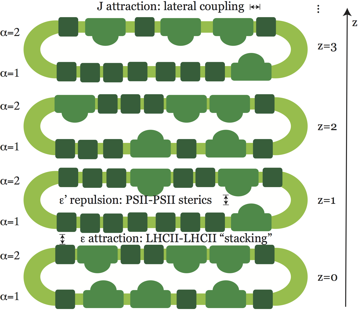
Figure 1: Schematic cross-section of a short stack of thylakoids discs. Dark green squares represent LHCII molecules, lighter green domed shapes represent PSII, and yellow-green bands represent lipid bilayers. Each disc (indexed by an integer $z$) comprises two layers (indexed $\alpha=1$ and $\alpha=2$). Protein attraction within each layer is assigned an energy scale $J$ in our lattice model. Aligned LHCIIs in subsequent layers can engage in favorable stacking interactions, which is assigned an energy $\epsilon$ in the model. Protrusion of PSII into the lumen spaces (i.e., the interior of each disc) may lead to steric repulsion between the two layers of each disc. Mediated by thylakoid gap and membrane fluctuations, the effective steric energy scale is denoted $\epsilon^{\prime}$.

IV Model

IV.1 Physical description

Our model of stacked thylakoid discs elaborates the familiar lattice gas model of liquid-vapor phase transitions. We represent the microscopic arrangement of proteins on a cubic lattice, resolving their transiently high number density in some parts of the membrane and low density in others. Proteins’ specific identities and internal structures are not resolved here; in discretizing space at the scale of a protein diameter, we have notionally averaged out such details. Our fluctuating degrees of freedom are thus binary variables $n$ for each lattice site, indicating the local scarcity ($n=0$) or abundance ($n=1$) of protein. We refer to the local states $n=0$ and $n=1$ as unoccupied and occupied, respectively, although they do not strictly indicate the presence of an individual molecule.

The net protein density in our model membranes may be specified explicitly, or else set indirectly through a chemical potential $\mu$ that regulates density fluctuations. For mathematical convenience we take the latter approach in most calculations, in effect allowing exchange of material with a reservoir. Here, the stroma lamellae – unstacked regions of photosynthetic membrane – could play the role of reservoir. For a real thylakoid stack, such exchange might be very slow, so that the largest-scale features of experimentally observed states are not well equilibrated. In that case, the phase transitions discussed below would not be manifested by coherent long-range order; instead, internally ordered domains would appear and grow, but their size would not reach a disc’s entire lateral area.

Interaction energies are assigned wherever adjacent sites on the lattice are occupied. The sign and strength of such an interaction depends on the locations of the two lattice sites involved, as depicted in Fig. 1. Within a planar layer of the stack (a disc comprises two layers), neighboring occupied sites contribute an attractive energy $-J$, representing lateral forces of protein-protein association. Stacking interactions occur between laterally aligned sites on the facing layers of sequential discs in the granum; each pair of occupied stacked sites contributes an attractive energy $-\epsilon$.

Laterally aligned sites within the same disc are subject to a repulsive energy $\epsilon^{\prime}$, representing steric forces between transmembrane proteins protruding into the lumen. The harshly repulsive nature of steric interactions suggests that $\epsilon^{\prime}$ should be very large, effectively enforcing a constraint of volume exclusion. For this reason, we will consider $\epsilon^{\prime}=\infty$ as a special case. Termed the hard constraint limit, this case offers mathematical simplification as well as transparent connections to a related class of spin models. Smaller values of $\epsilon^{\prime}$, however, may be more appropriate in situations where steric overlap can be avoided through modest deformation of the membrane layers. Under high light conditions, when thylakoid discs swell in the vertical direction, very slight membrane deformation (or perhaps none at all) could be sufficient to allow simultaneous occupation of laterally aligned sites, corresponding to very small $\epsilon^{\prime}$.

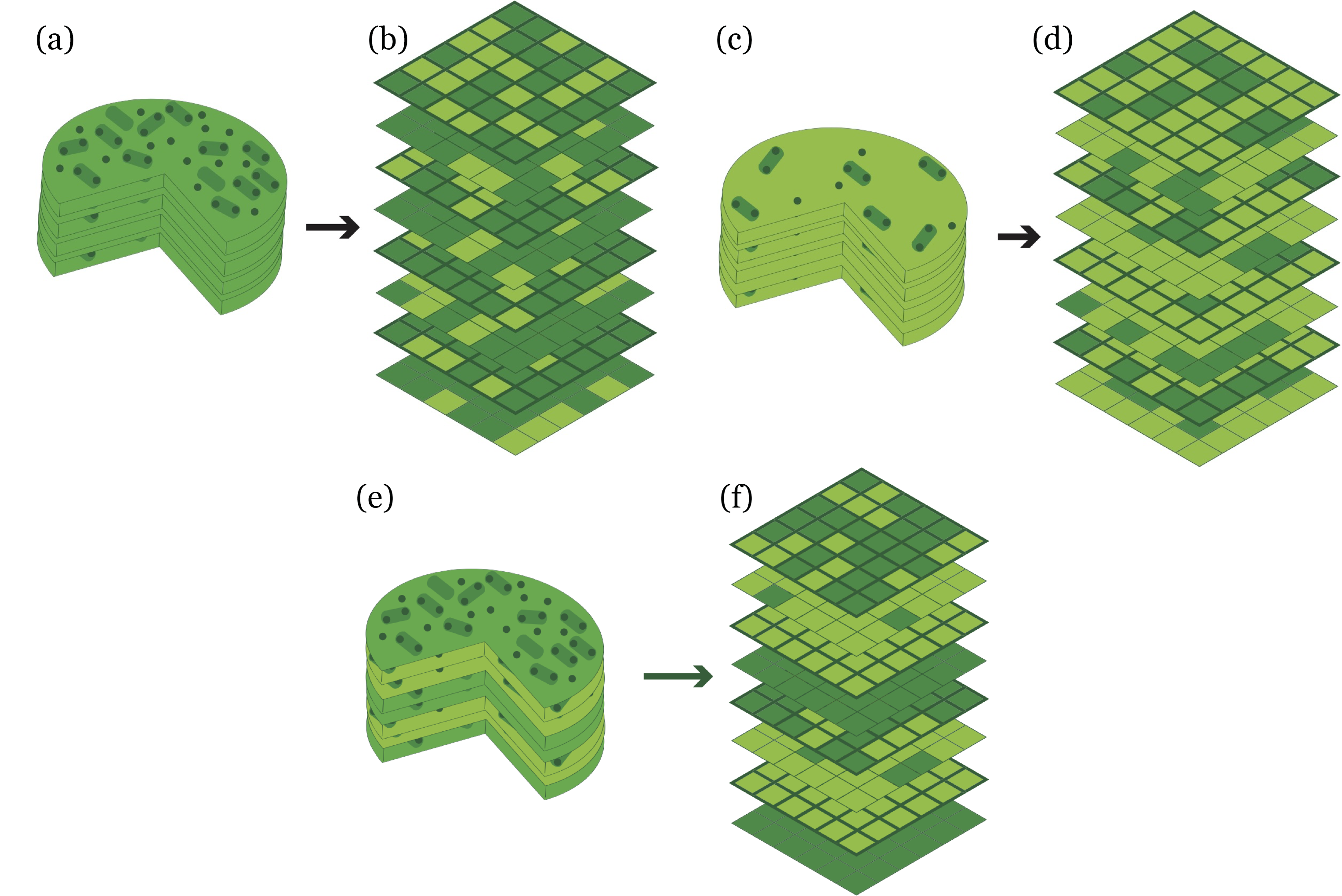
Figure 2: Illustrations of three different granum states ((a), (c), and (e)), and their representations in our lattice model ((b), (d), and (f)). In (a), (c), and (e), yellow-green indicates membrane that is not inhabited by protein; small dark circles are LHCII trimers; and oblong green shapes with small circles are PSII-LHCII supercomplexes. In (b), (e), and (f), yellow-green indicates a local sparsity of proteins, and dark green represents a region that is densely populated by either protein. These colors and shapes are used consistently throughout the paper. (a) and (b) depict a state of high average protein density in the granum. (c) and (d) depict a state of low average protein density. (e) and (f) illustrate a granum state with striped order. Here, layers of high and low protein density alternate vertically with a period of two discs. Each disc includes one high-density layer and one low-density layer; and each high-density layer is vertically adjacent to a dense layer on an adjacent disc.

The ground state of this model depends on values of the energetic parameters $\mu$, $\epsilon$, $J$, and $\epsilon^{\prime}$. Large, positive $\mu$ encourages the presence of proteins and thus favors a high average value $\bar{n}$ of the local occupation variable. In the limit $\mu\rightarrow+\infty$, a state of complete occupation is thus energetically minimum. At high but finite $\mu$ we generally expect thermodynamic states that are densely populated with protein, as depicted in Fig. 2 (a) and (b). Conversely, at very negative values of $\mu$ we expect very sparse equilibrium states, as depicted in Fig. 2 (c) and (d).

Equilibrium states at modest $\mu$ are characterized by competition among steric repulsion and the favorable energies of stacking and in-plane association. Large $\epsilon^{\prime}$ harshly penalizes lattice states that are more than half full – states which must feature simultaneous occupation of laterally aligned sites within the same disc. In order to realize in-plane attraction at half filling, one layer of each thylakoid must be depleted of protein. The stack then comprises a series of sparse and dense layers. Extensive stacking interaction between discs requires a coherent sequence of these layers, yielding ground states that are striped with a period of four layers. This pattern is illustrated in Fig. 2 (e) and (f), and is quantified by an order parameter $\Delta n$ that compares protein density in the two layers of each thylakoid. More specifically, $\Delta n$ is a linear combination of layer densities, whose coefficients change sign with the same periodicity as the stripe pattern described.

Macroscopically ordered stripes of protein density may be an unlikely extreme in real grana. Slow kinetics of protein exchange with stroma lamellae, imperfect grana architecture, or insufficiently strong interactions could all prevent long-range coherence in practice. The tendency towards ordering for dark to low light conditions can still be of importance, e.g., in the form of transient striping over substantial length scales or a steep decline in the population of vertically adjacent PSIIs as the transition is approached.

The two layers of each disc are completely equivalent in our model energy function. Stripe patterns, which populate the two layers differently with a persistent periodicity, do not possess this symmetry. Equilibrium states with $\Delta n\neq 0$ therefore require a spontaneous symmetry breaking and a macroscopic correlation length, and they must be separated from symmetric states by a phase boundary. The computational and theoretical work reported in the following sections aims to determine what, if any, thermodynamic conditions allow for such symmetry-broken, coherently striped states at equilibrium.

Our goals in exploring this model are both explanatory and functional. For grana at conditions that have been examined in experiment, we aim to explain observed trends in protein distribution based on simple, physically realistic interactions. Some interesting behaviors of our model, however, may be fully realized only at protein densities that are challenging to reach with existing experimental techniques. For these conditions, our results offer predictions for the emergence of spatial patterns that have not yet been observed. Possible physiological consequences of this organization will be discussed in Sec. VII.

IV.2 Mathematical definition

In order to describe quantitatively the energetics and ordering described above, we introduce: a label $z$ distinguishing different thylakoid discs, a label $\alpha$ distinguishing the two sides of each disc, and a label $i$ distinguishing positions within each membrane layer. The notation $n_{\alpha,i}^{(z)}$ for an occupation variable therefore indicates (a) the thylakoid disc to which it belongs, specified by a vertical coordinate $z$ ranging from 1 to $L_{z}$, (b) which layer of the disc it inhabits, $\alpha=1$ (bottom) or $\alpha=2$ (top), and (c) its lateral position, specified by an integer $i$ ranging from 1 to $L_{x}L_{y}$. (See Fig. 1). Density and striping order parameters are then defined as

$$\bar{n}\equiv(2L_{x}L_{y}L_{z})^{-1}\sum_{z,i,\alpha}n_{\alpha,i}^{(z)}$$ (1)

and

$$\Delta n\equiv(2L_{x}L_{y}L_{z})^{-1}\sum_{z,i}(-1)^{z}(n_{1,i}^{(z)}-n_{2,i}^{(z)}),$$ (2)

and the total energy of a configuration $\{n_{\alpha,i}^{(z)}\}$ is written

$$H[\{n_{\alpha,i}^{(z)}\}] =-\mu\sum_{z,\alpha}\sum_{i}n_{\alpha,i}^{(z)}-J\sum_{z,\alpha}\sum_{i,j}{}^{{}^{\prime}}n^{(z)}_{\alpha,i}n^{(z)}_{\alpha,j}$$ (3)

$$-\epsilon\sum_{z}\sum_{i}n^{(z)}_{2,i}n^{(z+1)}_{1,i}+\epsilon^{{}^{\prime}}\sum_{z}\sum_{i}n_{1,i}^{(z)}n_{2,i}^{(z)},$$

where the primed summation extends over distinct pairs of lateral nearest neighbors. As described above, each occupation variable $n_{\alpha,i}^{(z)}$ adopts values 1 (occupied) or 0 (unoccupied). The energetic parameters $\epsilon$ (in-plane attraction), $J$ (stacking attraction), and $\epsilon^{\prime}$ (steric repulsion) are all positive constants. At temperature $T$, the equilibrium probability distribution of $\{n_{\alpha,i}^{(z)}\}$ is proportional to the Boltzmann weight $e^{-\beta H}$, where $\beta\equiv 1/k_{B}T$.

In addition to transparent spatial symmetries, this model possesses a symmetry with respect to inverting occupation variables. Applying the transformation $\hat{n}_{\alpha,i}^{(z)}=1-n_{\alpha,i}^{(z)}$ to all lattice sites generates from any configuration $\{n_{\alpha,i}^{(z)}\}$ a dual configuration $\{\hat{n}_{\alpha,i}^{(z)}\}$ whose probability is also generally different from the original. As in the lattice gas, a certain choice of parameters renders the Boltzmann weight invariant under this transformation. In our case this statistical invariance occurs when $-2\mu-4J-\epsilon+\epsilon^{\prime}=0$, establishing a line of symmetry in parameter space. More usefully for our purposes, the duality establishes pairs of equilibrium states with related thermodynamic properties. Specifically, the states $(\mu,\epsilon,J,\epsilon^{\prime},T)$ and $(\hat{\mu},\epsilon,J,\epsilon^{\prime},T)$ have identical statistics of $\Delta n$ for the choice

$$\hat{\mu}=-\mu-4J-\epsilon+\epsilon^{\prime}$$ (4)

Viewing density rather than chemical potential as a control parameter, distributions of $\Delta n$ are identical in pairs of thermodynamic states $(\bar{n},\epsilon,J,\epsilon^{\prime},T)$ and $(\hat{\bar{n}},\epsilon,J,\epsilon^{\prime},T)$ related by $\hat{\bar{n}}=1-\bar{n}$; in other words, $\bar{n}=1/2$ is also a line of symmetry due to duality.

For the phase transitions of interest here, these arguments guarantee that any phase boundary at chemical potential $\mu$ (or density $\bar{n}$) is mirrored by a dual transition at $\hat{\mu}$ (or $\hat{\bar{n}}$), for any consistent choice of $\epsilon,J,\epsilon^{\prime}$, and $T$. More physically, any phase change induced by controlling protein density must exhibit reentrance (or else occur exactly at the line of symmetry, which we do not observe).

In simpler terms, imagine an initial equilibrium state with very low protein density and negligible spatial correlation. Increasing protein occupancy towards half filling could (and often does) drive the model system into a striped state with long range order. The inversion symmetry we have described dictates that a further increase in density must eventually destroy striped order. The latter transition may be more easily envisioned as a consequence of loading thylakoid discs beyond half filling – once steric energies have been overcome, the competition underlying striped order becomes imbalanced, and an unmodulated state of high density is thermodynamically optimal. Mathematically, the loss of modulated order at high protein density is simply the dual transition of its appearance.

Like the lattice gas, our thylakoid stack model can be mapped exactly onto a spin model with binary variables $\sigma=2n-1=\pm 1$. Among the expansive set of spin models that have been explored numerically and/or analytically, we are not aware of one that maps precisely onto this variant of the lattice gas. Many, however, share similar ordering motifs and spin coupling patterns. Ellis, Otto, and Touchette (2005); Deserno (1997); Ez-Zahraouy and Kassou-Ou-Ali (2004) Alternating attraction and repulsion in Eq. (3) correspond to mixed ferromagnetic and antiferromagnetic couplings in a spin model, e.g., in axial next-nearest neighbor Ising (ANNNI) models, which can also support modulated order. Fisher and Selke (1980) A different class of spin models seems better suited to the hard constraint limit of Eq. (3). For $\epsilon^{\prime}=\infty$ each lateral position on a thylakoid disc can adopt three possible states (both layers empty, and one or the other layer filled), two of which are statistically equivalent. The similarity to a three-state Potts model in an external field is more than superficial. Much of the phase behavior we identify echoes what is known for that model in three dimensions, Wu (1982) even for finite steric repulsion strengths ($\epsilon^{\prime}$).

The spirit of our approach echoes many previous efforts to understand basic physical mechanisms of collective behavior in membrane systems, from lipid domain formation to correlations among sites pinned by proteins or substrates. Speck, Reister, and Seifert (2010); Machta, Veatch, and Sethna (2012); Jho et al. (2011); West, Brown, and Schmid (2009); Naji and Brown (2007); Meilhac and Destainville (2011); Pasqua et al. (2010); Stachowiak et al. (2012); Schmid et al. (2016); Schick (2012); Garbès Putzel and Schick (2012); Heimburg (2007); Frazier et al. (2007); Yethiraj and Weisshaar (2007); Honerkamp-Smith et al. (2008); Machta et al. (2011); Mitra et al. (2018); Meerschaert and Kelly (2015) By stripping away most molecular details, simplified descriptions of phase transitions, such as spin models and field theories, focus attention on the emergence of dramatic macroscopic response from a few microscopic ingredients. They also greatly reduce the computational cost of sampling pertinent fluctuations, which are simply inaccessible for biomolecular systems near phase boundaries when considered in full atomistic detail. This perspective has even been applied to lipid ordering in stacks of membrane layers, but not in the context of protein ordering or photosynthesis. Tayebi et al. (2012); Tayebi, Parikh, and Vashaee (2013); Hoshino, Komura, and Andelman (2015, 2017)

Here we examine equilibrium structure fluctuations of the lattice model defined by Eq. (3), using both computer simulations and approximate analytical theory. We first describe results of Monte Carlo sampling, which confirm the stability of a striped phase over a broad range of temperature and density. We then present mean-field analysis that sheds light on the nature of symmetry breaking and relationships with previously studied models.

Symbol	Definition
$L_{x}$, $L_{y}$	Side length of the lattice in $x$ and $y$ directions
$L_{z}$	Number of thylakoid discs in granum stack
$z$	Thylakoid disc index ($1\leq z\leq L_{z}$)
$\alpha$	Bottom ($\alpha=0$) or top ($\alpha=1$) of a thylakoid disc
$i$	Location of a lattice site in the $xy$-plane of a disc ($1\leq i\leq L_{x}*L_{y}$)
$n_{\alpha,i}^{(z)}$	Presence ($n_{\alpha,i}^{(z)}=1$) or absence ($n_{\alpha,i}^{(z)}=0$) of proteins at a lattice site
$\beta$	Inverse temperature $(k_{B}T)^{-1}$
$J$	Strength of lateral protein attraction ($J>0$)
$\epsilon$	Strength of vertical stacking attraction ($\epsilon>0$)
$\epsilon^{\prime}$	Strength of vertical steric repulsion ($\epsilon^{\prime}>0$)
$\mu$	Protein chemical potential
$\bar{n}$	Average total density (see Eq. (1))
$\Delta n$	Striping order parameter (see Eq. (2))
$K$	Net strength of attraction, relative to thermal energy (see Eq. (5))
$F$	Free energy (see Eq. (VI.1.2))
$p_{n_{1}n_{2}}$	Probability of microstate $(n_{1},n_{2})$ of a two-site cluster
$\delta$	Boltzmann factor $e^{-\beta\epsilon^{\prime}}$ for steric repulsion
$K^{*}$	Attraction strength at which striping transition becomes discontinuous

Table 1: Key physical variables and parameters for the thylakoid lattice model.

V Methods and Results: Monte Carlo simulations

We used standard Monte Carlo methods to explore the phase behavior of our thylakoid lattice model. Specifically, we sampled the grand canonical probability distribution $e^{-\beta H}$ for a periodically replicated system with $L_{x}=L_{y}=10$ and $L_{z}=24$, over broad ranges of temperature and chemical potential. This geometry can accommodate $L_{z}/2=12$ copies of the striped motif in the central simulation cell.

Within mean field approximations presented in the next section, the attractive energy scales $J$ and $\epsilon$ are most important in the combination $4J+\epsilon$. We therefore define a parameter

$$K\equiv(4J+\epsilon)/k_{B}T$$ (5)

and focus on $\beta\mu$, $K$, and $\epsilon^{\prime}$ as essential control variables for this model. The ratio $J/\epsilon$ can also be varied; but for values of $J/\epsilon$ that are not extreme, this ratio is not expected to affect qualitative behavior. For simplicity, we limit attention to results exclusively for values of $J/\epsilon$ very close to 1/4, for which we have systematically varied $\beta\mu$, $K$, and $\epsilon^{\prime}$. A limited set of simulations with $J/\epsilon=0.5$ and 1 support the ratio $J/\epsilon$ as inessential within the range studied.

These simulations confirm the ordering scenario described above, in which the average value $\langle\Delta n\rangle$ of the striping order parameter can become nonzero in an intermediate range of $\beta\mu$. In other words, a phase with macroscopically coherent stripes can be thermodynamically stable at intermediate density. We identify and characterize transitions between this striped phase and the “disordered” phase with $\langle\Delta n\rangle=0$ by computing probability distributions $P(\Delta n)$. Fig. 3 shows corresponding free energy profiles $F(\Delta n)=-k_{\rm B}T\ln P(\Delta n)$ determined by umbrella sampling (see Supporting Material). For $2.6<K<6$, the progression from convexity to bistability of $F(\Delta n)$ as $\beta\mu$ increases at fixed $K$ and $\epsilon^{\prime}$ is suggestive of Ising-like symmetry breaking. Quantitative features of $F(\Delta n)$ support this connection. In particular, near the transition Binder cumulants approach values characteristic of 3-dimensional Ising universality (see Supporting Material). For $K>6$ thorough sampling of the equilibrium distribution becomes challenging, as acceptance probabilities decline due to strong interactions and striped domains become highly anisotropic. In the Supporting Material we present indirect evidence that the ordering transition becomes discontinuous at $K\geq 6$.

Over a wide range of interaction strength $K$, loading of proteins into the model thylakoid is thus accompanied by continuous transitions in $\langle\Delta n\rangle$, critical fluctuations, and correspondingly dramatic susceptibility. We locate this transition through the shape of the free energy profile. The striped phase is stable wherever $F(\Delta n)$ possesses global minima away from $\Delta n=0$. Elsewhere, the thylakoid is macroscopically disordered, though stripe patterns may be prominent on microscopic scales.

Fig. 4 shows the phase diagram in the $(K,\beta\mu)$ plane. An equivalent but more intuitive representation in the plane of $K$ and $\bar{n}$ is given in Fig. 5. Results are included for a broad range of $\epsilon^{\prime}$ values. In all cases, computed phase boundaries are lines of Ising-like critical points. All boundaries are mirrored across the lines of inversion symmetry of Eq. (4), or $\bar{n}=1/2$ in the $\bar{n}$ vs. $K$ plane, respectively. As described in Sec. IV.2, striping transitions at finite $\epsilon^{\prime}$ are consequently re-entrant for all finite steric repulsion strengths $\epsilon^{\prime}$. Modulated order requires sufficient filling of the lattice but is inevitably destroyed by high density.

The shapes of these phase diagrams clearly reflect the origin of modulated order in an interplay between proteins’ attraction and steric repulsion. The domain of stability of the striped phase is largest where attraction and repulsion are both potent (i.e., $\beta\epsilon^{\prime}$ and $K$ are both much greater than unity). Small values of either $\beta\epsilon^{\prime}$ or $K$ greatly compromise this stability, or eliminate it entirely.

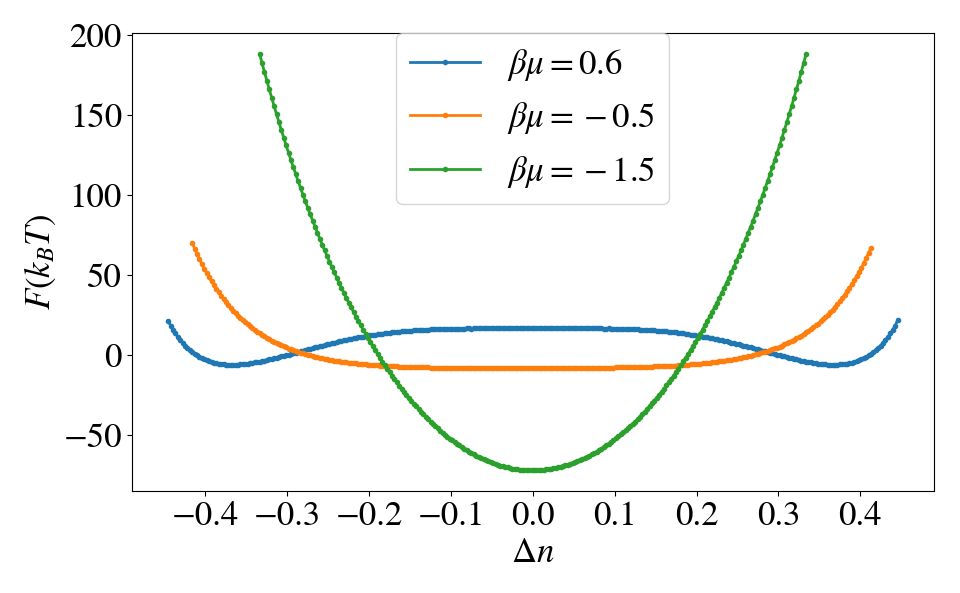
Figure 3: Statistics of the striping order parameter $\Delta n$ at three different thermodynamic states. In all cases Monte Carlo simulations were performed with $\epsilon^{\prime}=20k_{B}T$, $J=0.4k_{B}T$, $\epsilon=1.65k_{B}T$ (corresponding to $K=3.25$), $L_{z}=24$, and $L_{x}=L_{y}=10$. The free energy relative to thermal energy, $\beta F=-\ln{P(\Delta n)}$, is shown for $\beta\mu=-1.5$, $\beta\mu=-0.5$, and $\beta\mu=0.6$. For the highest value of $\beta\mu$, macroscopic bistability indicates a striped state with long-ranged order and broken symmetry. For the lowest value of $\beta\mu$, Gaussian fluctuations in $\Delta n$ typify the sparse disordered state. For the intermediate value of $\beta\mu$, the quartically flat shape of $\beta F$ near $\Delta n=0$ indicates proximity to a continuous ordering transition.

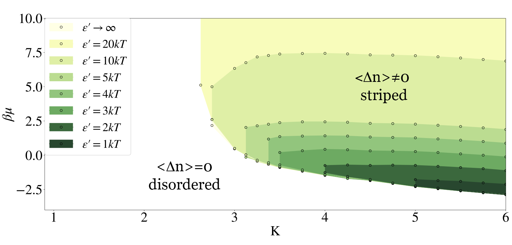
Figure 4: Phase diagrams of the thylakoid lattice model constructed from Monte Carlo simulation results, shown in the plane of attraction strength and chemical potential. Results are shown for several values of repulsion strength $\epsilon^{\prime}$. In the white region, the disordered phase is stable for all $\epsilon^{\prime}$. The region with darkest shading shows the range of $\beta\mu$ and $K$ over which the ordered phase is stable for $\beta\epsilon^{\prime}=1$. The next darkest region shows the additional range of ordered phase stability at $\beta\epsilon^{\prime}=2$, and so on. All phase boundaries, which are assumed to follow straight lines between explicitly determined points (circles), mark continuous striping transitions. Results for the hard constraint limit, $\epsilon^{\prime}=\infty$, are indistinguishable from those with $\beta\epsilon^{\prime}=20$.

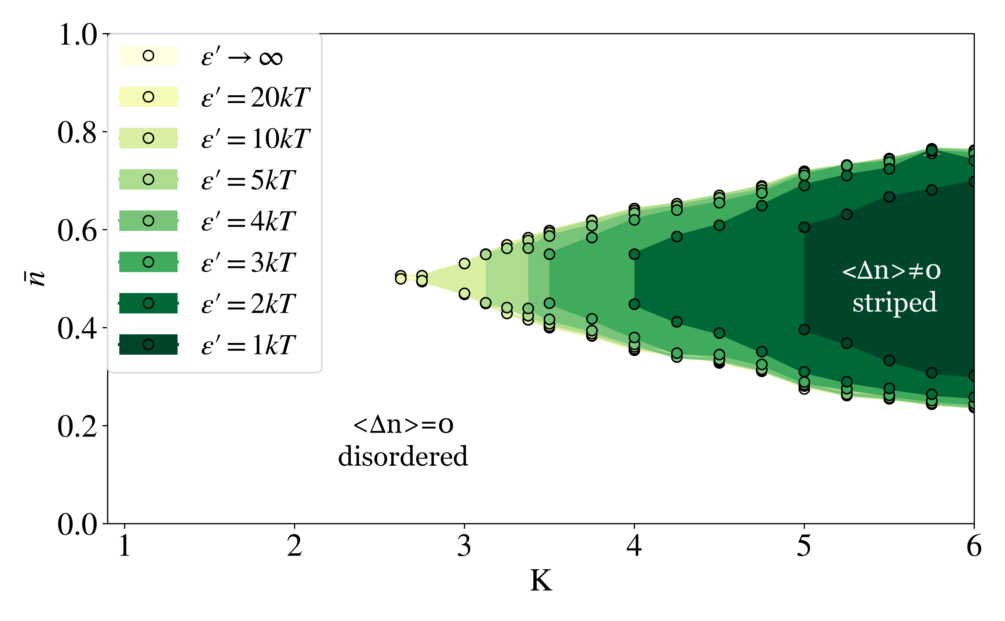
Figure 5: Phase diagrams of the thylakoid lattice model constructed from Monte Carlo simulation results, shown in the plane of attraction strength and density. Points and shading have the same meaning as in Fig. 4 Results for the hard constraint limit, $\epsilon^{\prime}=\infty$, are indistinguishable from those with $\beta\epsilon^{\prime}=20$. For the latter case, $\beta\epsilon^{\prime}=20$, we did not impose high enough chemical potential in simulations to obtain results for $\bar{n}>1/2$. In the hard constraint limit, the regime $\bar{n}>1/2$ is strictly forbidden.

VI Methods and Results: Mean field theory

As with most critical phenomena, the long-ranged correlation of protein density fluctuations implied by these phase transitions greatly hinders accurate analytical treatment. Here we employ the most straightforward of traditional approaches for predicting phase behavior, namely mean field (MF) approximations, to further explore and explain the ordering behavior revealed by Monte Carlo simulations of the thylakoid model. Though quantitatively unreliable in general, mean-field methods provide a simple accounting for the collective consequences of local interactions, and thus a transparent view of phase transitions that result.

Mean field theories generically treat the fluctuations of select degrees of freedom explicitly, regarding all others as a static, averaged environment. We first consider a pair of fluctuating lattice sites in a self-consistent field, whose continuous transitions can be easily inferred. We then analyze an extended subsystem of 12 tagged lattice sites, whose qualitative predictions align with the simpler treatment. This consistency suggests a robustness of mean-field predictions for the thylakoid model.

VI.1 Two-site clusters

In order to describe modulated order of the striped phase, a subsystem for mean field analysis should include representatives from both layers of a thylakoid disc. Our simplest approximations therefore focus on a pair of tagged occupation variables, $n_{1,1}^{(1)}$ and $n_{2,1}^{(1)}$, describing density fluctuations at vertically neighboring lattice sites that interact directly through steric repulsion. We will describe mean field analysis for this two-site cluster first in the simplifying case $\epsilon^{\prime}\rightarrow\infty$, i.e., the hard constraint limit. We then consider the more general case of finite repulsion strength.

VI.1.1 Hard constraint limit

In the limit $\epsilon^{\prime}\rightarrow\infty$, the microstate $n_{1,1}^{(1)}=n_{2,1}^{(1)}=1$ of our two-site cluster is prohibited. As a result, the mean field free energy $F_{\rm MF}$ can be written very compactly. We construct $F_{\rm MF}$ from (a) the Gibbs entropy associated with probabilities of the cluster’s three allowed microstates and (b) the average energy of interaction with a static environment. In terms of the order parameters $\bar{n}$ and $\Delta n$, we obtain

$$\frac{2\beta F_{\rm MF}}{N} =-2\beta\mu\bar{n}+(\bar{n}+\Delta n)\log(\bar{n}+\Delta n)$$ (6)

$$+(\bar{n}-\Delta n)\log(\bar{n}-\Delta n)$$

$$+(1-2\bar{n})\log(1-2\bar{n})-K(\bar{n}^{2}+\Delta{n}^{2}),$$

where $N$ is the total number of lattice sites. Eq. (6) suggests a close relationship between our thylakoid model and the well-studied 3-state Potts model of interacting spins. Applying the Curie-Weiss MF approach to that Potts model yields a free energy of identical form to Eq. 6 for the case of an external field that couples symmetrically to two of the spin states. Wu (1982) The MF phase behavior of the two models is therefore isomorphic, involving both first-order and continuous symmetry-breaking transitions. The continuous transitions are qualitatively consistent with results of our Monte Carlo sampling. The discontinuous transitions were not observed in thylakoid model simulations for $K<6$; evidence for them emerges only for larger values of $K$, where sampling becomes challenging.

Continuous transitions may be identified by expanding Eq. (6) for small $\Delta n$. This expansion indicates a local instability to symmetry-breaking fluctuations that first appears at $\bar{n}=K^{-1}$. A corresponding phase boundary in the $(K,\beta\mu)$ plane can then be found by minimizing $F_{\rm MF}$ with respect to $\bar{n}$, yielding $\beta\mu=-1-\ln(K-2)$. This result, plotted as the black curve in Fig. 6, captures the most basic features of our simulation results at large $\beta\epsilon^{\prime}$. As is typically true, the maximum temperature at which ordering occurs is overestimated by MF theory (i.e., the minimum value of $K$ is underestimated).

For sufficiently large $K$, numerical minimization of $F_{\rm MF}$ reveals transitions that are instead discontinuous, as shown by the red curve in Fig. 6. Here, the disordered state remains locally stable while global minima emerge at nonzero $\Delta n$. The onset of such transitions at $K^{*}=10/3$ can be determined by careful Taylor expansion of $F_{\rm MF}$ in powers of $\bar{n}$ and $\Delta n$ (see Supporting Material). Both of these order parameters suffer discontinuities at the first-order phase boundary. For $K<K^{*}$, no discontinuous transitions are observed (in Fig. 6, the red curve thus begins at $K^{*}$).

The absence of first-order transitions in computer simulations near $K=10/3$ could signal a failure of this simple mean field theory. Alternatively, such transitions may occur only at higher values of $K$. This low-temperature regime is challenging to explore with our Monte Carlo sampling methods. Below we will show that discontinuous transitions survive in more sophisticated MF treatments, suggesting they are a real feature of the model that is difficult to access with simulations.

Both simulations and MF theory indicate that the striping transition is not re-entrant in the hard constraint limit. High-density disordered states are prohibited by steric repulsion at $\epsilon^{\prime}=\infty$.

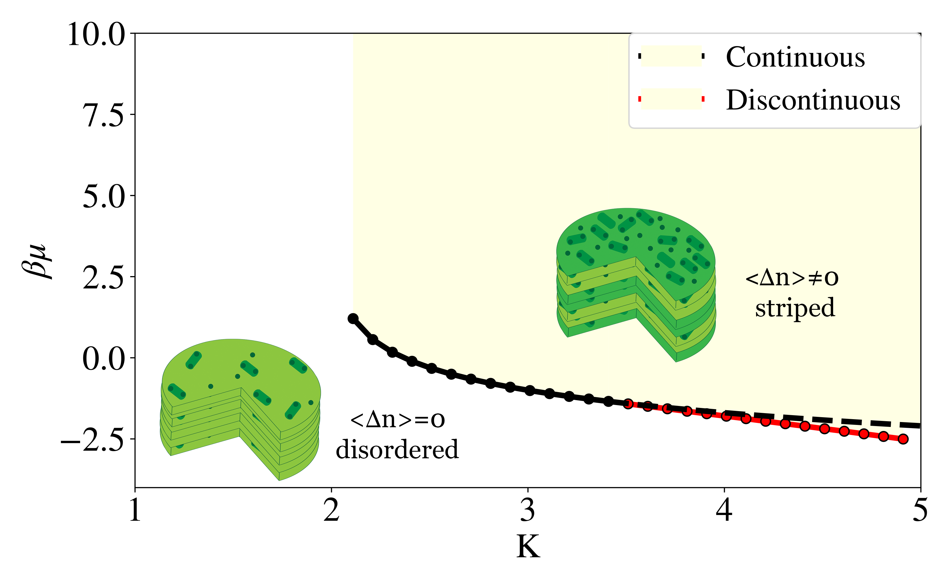
Figure 6: Phase diagram of the thylakoid lattice model determined from mean field theory in the hard constraint limit $\epsilon^{\prime}=\infty$, shown in the plane of attraction strength and chemical potential. In the white region, Eq. 6 has a single minimum, at $\Delta n=0$, indicating a lack of striped order. In the shaded region, global minima at nonzero $\Delta n$ indicate symmetry breaking, i.e., striping with long-range coherence. The extremum of $F_{\rm MF}$ at $\Delta n=0$ changes stability at the black curve, allowing for continuous ordering. At large $K$ this continuous change is preempted by a first-order transition (red curve).

VI.1.2 Soft steric repulsion

The same basic MF approach can be followed for finite $\epsilon^{\prime}$. In this case, however, $F_{\rm MF}$ is written most naturally not as a function of $\bar{n}$ and $\Delta n$, but instead in terms of probabilities $p_{n_{1}n_{2}}$ for the four possible cluster microstates:

$$\frac{2\beta F_{\rm MF}}{N} =p_{00}\ln p_{00}+p_{10}\ln p_{10}+p_{01}\ln p_{01}+p_{11}\ln p_{11}$$

$$-\frac{K}{2}[(p_{11}+p_{10})^{2}+(p_{11}+p_{01})^{2}]$$

$$+\beta\epsilon^{\prime}p_{11}-\beta\mu(p_{10}+p_{01}+2p_{11})$$ (7)

Recognizing that $\Delta n=(p_{10}-p_{01})/2$ and $\bar{n}=(p_{10}+p_{01}+2p_{11})/2$, expansion and minimization of Eq. (VI.1.2) yields continuous transitions in the $(K,n)$ plane along

$$\bar{n}=\frac{1}{2}\pm\frac{1}{2K}\sqrt{(K-2)^{2}-4\delta}$$ (8)

where $\delta=e^{-\beta\epsilon^{\prime}}$. The two values of $\bar{n}$ for each $K>2(1+\sqrt{\delta})$ mark transitions to the low- and high-density disordered phases, reflecting the occupation inversion symmetry discussed in Sec. IV.2. In the $(K,\beta\mu)$ plane these transitions occur at

$$\beta\mu=\beta\epsilon^{\prime}-K\bar{n}+\ln{(K\bar{n}-1)}$$ (9)

where $\bar{n}$ refers to either solution of Eq. 8. Viewed as functions of $K$ at given $\epsilon^{\prime}$, the two branches of $\beta\mu$ in Eq. 9 have the peculiar feature of crossing at a certain attraction strength $K=K_{\rm cross}(\epsilon^{\prime})$ (see Supporting Material). For $K>K_{\rm cross}$ these solutions violate fundamental stability criteria of thermodynamic equilibrium (see Supporting Material) and therefore cannot be global minima of the free energy. Lower-lying minima indeed appear at $K^{*}<K_{\rm cross}$, preempting the continuous ordering transition before the two solutions cross.

The development of nonzero $\langle\Delta n\rangle$ with increasing density is thus predicted to become discontinuous at sufficiently low temperature, as in the hard constraint case. The onset of this first-order transition,

$$K^{*}=\frac{10}{3}+\frac{2}{3}\delta+{\cal O}(\delta^{2}),$$ (10)

can be determined by Taylor expansion of $F_{\rm MF}$ in the regime of strong repulsion, i.e., large $\epsilon^{\prime}$ and small $\delta$. Figs. 7 and 8 show mean field phase diagrams for several values of $\epsilon^{\prime}$, as determined by numerical minimization of Eq. VI.1.2. For this mean field method, it is unnecessary to assume a value for $J/\epsilon$, as the mean field blurs distinctions between vertical and in-plane couplings for sites coupled via $J$ or $\epsilon$. As in the simulation results of Figs. 4 and 5, the data in Figs. 7 and 8 exhibit the symmetry guaranteed by duality. Discontinuous changes in density upon striping imply regions of coexistence in the plane of $K$ and $\bar{n}$. For densities that lie between average values for the ordered and disordered states, both phases are present at equilibrium, as indicated in Fig. 8, separated by an interface.

The domain of stability of the striped phase in mean field theory evolves with $\epsilon^{\prime}$ in the same basic way observed in Monte Carlo simulations. Relative to simulations, however, mean field results are consistently shifted to lower $K$ (higher $T$), increasingly so as $\epsilon^{\prime}$ decreases. The discontinuous nature of mean-field transitions at high $K$ is not easily corroborated by simulations, as sampling becomes challenging at high $K$. Limited simulations with very strong interactions suggest that first-order transitions appear between $K=6$ and $K=7$, in contrast to the mean field crossover prediction of $3<K^{*}<4$. Consequently, the coexistence regions displayed in Fig. 8 for mean field theory do not appear in simulation for $K<6$.

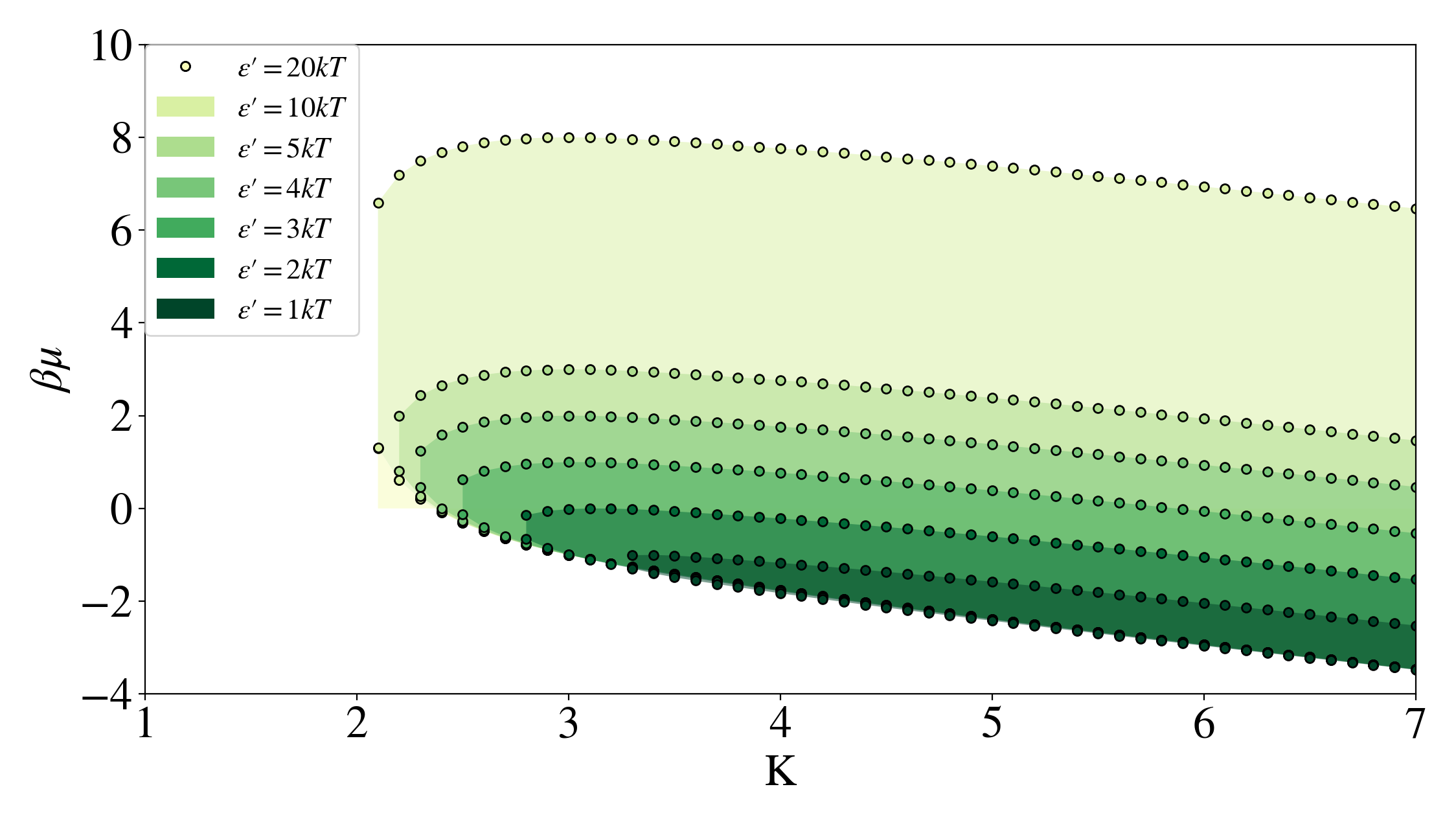
Figure 7: Mean-field phase diagram of the thylakoid lattice model at finite $\epsilon^{\prime}$, shown in the $(K,\beta\mu)$ plane. Shading has the same meaning as in Fig. 4. Phase boundaries, determined by minimizing Eq. VI.1.2, are continuous at small $K$ and discontinuous beyond a value $K^{*}$ that is well approximated by Eq. 10.

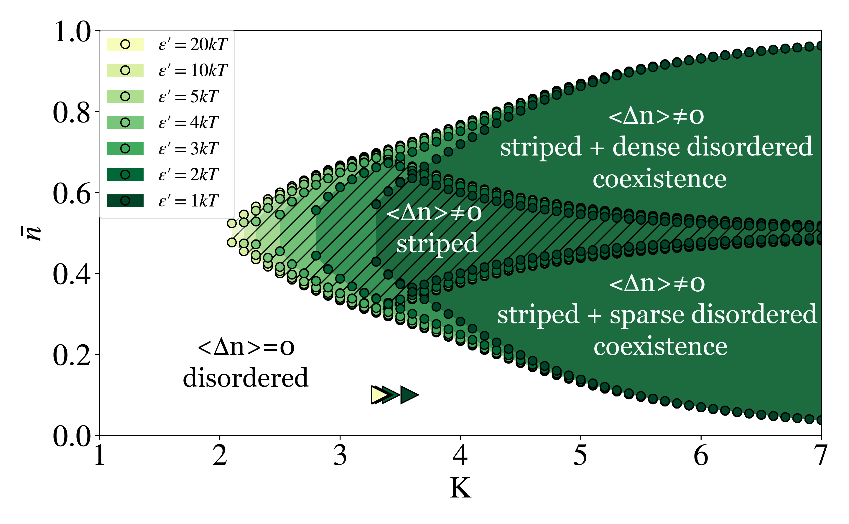
Figure 8: Mean-field phase diagram of the thylakoid lattice model at finite $\epsilon^{\prime}$, shown in the $(K,\bar{n})$ plane. Hatched regions indicate the striped phase, and the coloration corresponds to that of Fig. 4. Shaded but un-hatched regions mark coexistence between striped and disordered phases. Phase boundaries, determined by minimizing Eq. VI.1.2, are continuous at small $K$ and discontinuous beyond a value $K^{*}$ (indicated by triangle markers, with the same color as corresponding $\epsilon^{\prime}$) that is well approximated by Eq. 10.

VI.2 Bethe-Peierls approximation

The accuracy of MF theory is generally improved by examining a larger set of fluctuating degrees of freedom. Fair (1965) In some cases, considering large clusters can even remove spurious transitions suggested by lower-level calculations. MF treatments of anisotropic Ising models, some of which incorrectly predict discontinuous transitions, are particularly interesting here. Neto et al. have surveyed an array of MF approaches for one such model in two dimensions, which supports modulated order at low temperature. The simplest MF calculations predict a crossover from continuous to discontinuous ordering. The Bethe-Peierls (BP) approximation, a more sophisticated MF approach, captures the strictly continuous ordering observed in computer simulations.Neto, dos Anjos, and de Sousa (2006)

We have performed BP analysis for the thylakoid model (in 3 dimensions), in order to test the robustness of phase behavior predicted by the two-site calculations described above. Here, we enumerate all microstates of a subsystem that includes $n_{1,1}^{(1)}$, $n_{2,1}^{(1)}$, and all of their remaining nearest neighbors, a total of 12 sites. The additional sites experience effective fields representing interactions that are not explicitly considered. For the specific case $J=\epsilon$, only two of these fields may be distinct, greatly simplifying the self-consistent procedure. We focus exclusively on this case. The calculation and phase diagrams that result are presented in Supporting Material.

Like simpler MF approaches, the BP approximation yields several solutions for the effective fields at low temperature. Some of these solutions correspond to continuous ordering transitions, which can also be identified by Taylor expansion of the self-consistent equations. Other solutions describe symmetry-broken states that do not appear continuously, resembling in many respects the first-order transitions predicted by two-site calculations. Demonstrating that these states are thermodynamic ground states would require formulating a free energy for this BP approach, which we have not pursued. Their local stability, however, is clearly preserved in the BP scheme.

The most pronounced difference between BP phase diagrams and those of simpler MF treatments is a shift of phase boundaries to lower temperature (higher $K$). Agreement with Monte Carlo simulations is therefore improved. With this shift, the onset of discontinuous ordering transitions suggested by BP calculations occurs near $K=6$. This result supports the notion that first-order transitions are a real feature of the thylakoid model, occurring near the temperature range suggested by flat histogram sampling; see Supporting Material.

VII Discussion

The model we have constructed to study vertical arrangement of proteins in grana stacks is deliberately sparse in microscopic detail. It does not distinguish among the associating protein species in photosynthetic membranes, nor does it account for shape fluctuations of lipid bilayers in which these proteins reside. These unresolved features are undoubtedly important for the physiological consequences of the ordering scenario we have described, but they are inessential to its origins. The finite size of grana stacks is also neglected here. Sharp transitions we have described would be rounded in real thylakoids by finite size effects, but natural photosynthetic membranes should be large enough to exhibit micron-scale cooperativity in protein rearrangements.

A model that distinguishes among LHCII, PSII, and their super-complexes, we assert, should exhibit the same basic phase behavior as our coarse-grained representation, so long as it incorporates the same fundamental competition between attraction and repulsion. But such a model would be much less amenable to the theoretical and computational analyses we have presented, particularly if it acknowledges the differences in these proteins’ sizes and shapes. PSII proteins are typically more oblong and significantly larger than LHCII proteins; these two species also extend from the membrane layer to different degrees, influencing their interactions with proteins on both adjacent sides. Capturing these geometric features would greatly complicate a lattice representation. It would also require commensurately detailed parameterization of protein-protein interactions; given the scarcity of experimental information, locating physiologically relevant regions of parameter space would be even more challenging than for our lattice description. In conducting such a broad survey with a computationally demanding model, the existence and stability of an ordered phase could easily escape discovery altogether.

The lattice model of Eq. (3) is thus well-suited to reveal the existence and basic nature of vertical ordering in a system with the geometry and varied interactions of a stack of thylakoid membranes, which is the focus of this paper. Confidently establishing the conditions at which ordering occurs, and assessing its functional implications, calls for models with greater microscopic detail, like that of Ref.Schneider and Geissler (2013, 2014); Schneider (2013). In particular, distinguishing among LHCII, PSII, and super-complexed PSII-LHCII would enable correlation of vertical ordering with protein speciation. It would similarly help to explore connections between vertical ordering and the emergence of horizontally extended arrays of PSII-LHCII supercomplexes. Previous work suggests that such lateral ordering can be significantly stabilized by stacking attractions between thylakoid layers whose PSIIs are appropriately aligned Standfuss et al. (2005); Daum et al. (2010); Nield et al. (2000); Boekema et al. (2000), providing a natural mechanism of communication between these modes of organization.

In models that distinguish among different protein species, a thylakoid’s protein composition, and the LHCII:PSII ratio in particular, will figure importantly in any ordering scenario. If, maintaining the same net protein density, the concentration of LHCII were increased uniformly throughout the central region of a granum stack, the balance between steric forces (involving PSII) and stacking attraction (involving LHCII) would shift. In the language of our lattice model, the effective value of $K$ would increase, and $\epsilon^{\prime}$ would proportionally decrease. By looking at Figs. 5 and  8, one can see that in the density range $0.5\leq\bar{n}\leq 0.8$, this compositional shift would favor either the striped phase, or a coexistence of striped and disordered dense phase, depending on the magnitude of $K$. For densities greater than 0.8 and sufficiently large $K$, the system would enter the coexistence of striped and dense disordered phase.

Our model predicts that, at moderate to high protein density, LHCII stacking and PSII volume exclusion can induce coexistence between vertically striped and uniform phases in a stack of many membrane layers. Interestingly, previous work suggests that high density favors a coexistence scenario for lateral ordering as well. According to both experimental and computational studies, the extent of lateral ordering is quite sensitive to protein packing fraction. High density of LHCII in particular is known to destabilize lateral ordering. Schneider and Geissler (2013, 2014); Schneider (2013); Jansson et al. (1997); Veerman et al. (2007); Kirchhoff et al. (2007b); Murphy (1986); Kirchhoff et al. (1986); Haferkamp et al. (2010); Kouřil et al. (2013) Computational studies suggest that, under such circumstances ($0.65\leq\bar{n}\leq 0.85$, with LHCII:PSII at most 5:1), crystalline ordered phases should appear only in coexistence with fluid phases.Schneider and Geissler (2013, 2014); Schneider (2013) Physiologically relevant packing fractions can be similarly high (in the range 0.6-0.8), and measured LHCII:PSII ratios are in the range 2-6Jansson et al. (1997); Veerman et al. (2007); Kirchhoff et al. (2007b); Murphy (1986); Kirchhoff et al. (1986); Haferkamp et al. (2010); Kouřil et al. (2013), suggesting that coexistence between crystalline order and laterally disordered phases predominates both in vitro and in vivo. A tendency for phase separation in the context of both vertical and lateral ordering suggests that even weak coupling between the two could induce strong correlation.

The biological relevance of structural rearrangements predicted by our thylakoid model depends on the effective physiological values of parameters like $K$, $\epsilon^{\prime}$, and $\beta\mu$. Inherent weakness of attraction or repulsion, or else extreme values of protein density, could prevent thylakoids from adopting a striped phase. Photosynthetic membranes, however, visit states in the course of normal function that vary widely in protein density and in features that control interaction strength. We therefore expect significant excursions in the parameter space of Figs. 4 and 5. Since ordering transitions in our model require only modest density and interactions not much stronger than thermal energy, we expect proximity to phase boundaries to be likely in natural systems. Biological relevance depends also on the functional consequences of striped order. Photochemical kinetics and thermodynamics are determined by details of microscopic structure that we have made no attempt to represent, in particular, gradients in $pH$. If those aspects of intramolecular and supermolecular molecular structure are sensitive to local protein density or to the nanoscale spacing between dense regions, then striping transitions could provide a way to switch sharply between distinct functional states.

Given the limited availability of thermodynamic measurements on photosynthetic membranes, making quantitative estimates of the control variables $K$, $\epsilon^{\prime}$, and $\beta\mu$ for real systems is very challenging. We will focus on the current qualitative knowledge of properties that are conjugate to these parameters, in order to explore which phases could be pertinent to which functional states.

The majority of precise measurements on grana have assessed the density of specific proteins, which is of course conjugate to their chemical potential. For this reason we have presented phase diagrams in terms of both $\beta\mu$ and $\bar{n}$. Densities in central grana tend to be quite high, relative to other biological membranes. Combining information about the number density of PSII (from AFM or EM images) with measured number densities or stoichiometries of other protein species relative to PSII (typically measured by gel electrophoresis), packing fractions approach $\bar{n}\approx 0.6-0.8$. Schneider (2013); Kouřil et al. (2013); Haferkamp et al. (2010); Kirchhoff et al. (1986); Murphy (1986) Therefore, the top half of Figs. 5 and  8 are likely the most relevant for biology.

The net attraction strength relative to temperature, $K$, is conjugate to the extent of protein association within each membrane layer and across the stromal gap. Because experiments suggest stacking interactions have an empirically measured, dramatic effect on protein association, Chow et al. (2005); Standfuss et al. (2005); Phuthong et al. (2015); Onoa et al. (2014); Ruban and Johnson (2015) we will focus on the extent of stacking as a rough proxy for $K$. Previous computational work suggests that the range of $K$ we have explored is physiologically reasonable. Focusing on lateral protein ordering in a pair of membrane layers, Refs. Schneider and Geissler (2013); Schneider (2013) found that configurations consistent with atomic force microscopy images could be obtained for weak in-plane protein-protein attractions of energy $\leq 2k_{B}T$ and stacking energy $4k_{B}T$. Associating the energy scales of that particle model with the energies of our more coarse-grained lattice representation ($\beta J\lesssim 2$ and $\beta\epsilon\approx 4$) suggests values of $K$ in the neighborhood of 5-10. Ordering at moderate to large $K$ is therefore likely to be most physiologically relevant. It is in this regime that we find a evidence for a crossover in the nature of the striping transition, from continuous to discontinuous.

The strength of steric repulsion, $\epsilon^{\prime}$, is strongly influenced by thylakoid geometry. For a very narrow lumen and very rigid lipid bilayers, PSII molecules on opposite sides of a thylakoid disc are essentially forbidden to occupy the same lateral position, a hard constraint that is mimicked by the limit $\epsilon^{\prime}=\infty$ of Sec. VI.1.1. Greater luminal spacing, together with membrane flexibility, abates or possibly nullifies this repulsion. We therefore regard thylakoid width as a rough readout of $\epsilon^{\prime}$. Since thylakoid width changes significantly as light conditions change, we also view $\epsilon^{\prime}$ as a control variable related to light intensity. Each thylakoid is roughly 10-15 nm thick, and the lumenal gap measures approximately 2-7 nm, depending on light conditions. Dekker and Boekema (2005); Pribil, Labs, and Leister (2014); Nevo et al. (2012)

In high light conditions, the luminal gap of the thylakoid discs widens. Puthiyaveetil et al. (2014); Kirchhoff et al. (2012) This geometric change should ease steric repulsion, though lumen widening is less substantial at the center of the discs than at their edges. Clausen et al. (2014); Iwai et al. (2013) If the light intensity is particularly high, this expansion can be accompanied by the disassembly of PSII-LHCII mega-complexes (and, to a much lesser extent, super-complexes) en route to PSII repair. Erickson, Wakao, and Niyogi (2015); Puthiyaveetil et al. (2014); Kirchhoff et al. (2012); Herbstová et al. (2012); Koochak et al. (2019) Although this disassembly is primarily limited to the edges of the thylakoid, we infer an overall decrease in the extent of stacking. And because PSII is subsequently shuttled to the stroma for repair, we also expect a concomitant decrease in protein density. The implied low to modest values of $\beta\mu$, $\epsilon^{\prime}$, and $K$ suggest that high light scenarios favor the sparse disordered phase of our model.

In low light conditions, thylakoid discs are thinner, and the stromal gaps between them decrease as well Dekker and Boekema (2005); Pribil, Labs, and Leister (2014), pointing to large values of $\epsilon^{\prime}$ and $K$. The low-light state thus appears to be the strongest candidate for the striped phase we have described.

During state transitions, a collection of changes causes the balance of electronic excitations to shift from PSII to photosystem I. Erickson, Wakao, and Niyogi (2015); Clausen et al. (2014); Iwai et al. (2013); Minagawa (2011); Lemeille and Rochaix (2010). Among these changes, a diminution of stacking and a shift of LHCII density towards the stroma lamellae are closely related to the ordering behavior of our thylakoid model. Both result from phosphorylation of some fraction of the LHCII population, which weakens attraction between discs, prompts disassembly of a fraction of PSII-LHCII mega-complexes and super-complexes, and allows LHCII migration towards the thylakoid margins. The corresponding reduction of $\beta\mu$ and $K$ is likely to be highly organism-dependent, since the extent of phosphorylation varies greatly from algae to higher plants. Iwai et al. (2013); Minagawa (2011); Lemeille and Rochaix (2010); Wlodarczyk et al. (2016); Crepin and Caffarri (2015); Nawrocki et al. (2016) Lacking as well quantitative information about thylakoid thickness, it is especially difficult to correlate state transitions with the phase behavior of our model. In the case of very limited phosphorylation (as in higher plants), the ordered and sparse disordered phases both seem plausible. With extensive phosphorylation (as in algae), substantial reductions in stacking attraction and density make the ordered state unlikely.

The relationship among granum geometry, protein repulsion strength, and long-range stripe order suggests interesting opportunities for manipulating the structure and function of thylakoid membranes in vivo. By adjusting the luminal spacing, mechanical force applied to a stack of discs in the vertical direction (i.e., the direction of stacking) should serve as a handle on the steric interaction energy $\epsilon^{\prime}$. The phase behavior of our model suggests that smooth changes in force can induce very sharp changes in density, protein patterning, and stack height. Ref. Clausen et al. (2014) demonstrates a capability to manipulate thylakoids in this way, and could serve as a platform for testing the realism of our lattice model. Complementary changes in attraction strength might be achieved by controlling salt concentration, a strategy used in Ref. Kirchhoff et al. (2007a) to examine the influence of stacking interactions on lateral ordering of proteins in a pair of thylakoid discs.

VIII Conclusion

The computer simulations and analysis we have presented establish that ordered stripes of protein density, coherently modulated from the bottom to the top of a granum stack, can arise from a very basic and plausible set of ingredients. Most important is the alternation of attraction and repulsion in the vertical direction, a feature that is strongly suggested by the geometry of thylakoid membranes. Provided the scales of these competing interactions are both substantial, a striped state with long-range order will dominate at moderate density. Under conditions accessible by computer simulation, the striping transition is continuous, with critical scaling equivalent to an Ising model or standard lattice gas. Mean-field analysis suggests that the transition becomes first-order for strong attraction, switching sharply between macroscopic states but lacking the macroscopic fluctuations of a system near criticality.

Simple mechanisms for highly cooperative switching have been proposed and exploited in many biophysical contexts, Stachowiak et al. (2012); Schmid et al. (2016) including the lateral arrangement of proteins in photosynthetic membranes. Nevo et al. (2012); Liguori et al. (2015); Kirchhoff et al. (2007a); Erickson, Wakao, and Niyogi (2015); Puthiyaveetil et al. (2014); Clausen et al. (2014); Herbstová et al. (2012); Minagawa (2011); Lemeille and Rochaix (2010); Wlodarczyk et al. (2016); Nawrocki et al. (2016) We suggest that vertical ordering in stacks of such membranes can be a complementary mode of collective rearrangement with important functional consequences.

IX Author Contributions

A.M.R. performed all of the Monte Carlo simulations except the flat histogram sampling, numerical solutions, data analysis, and figure generation, as well as developed all the necessary software. P.L.G. provided guidance in these tasks and performed the flat histogram sampling in the Supporting Material. A.M.R. and P.L.G. authored this manuscript.

X acknowledgments

We acknowledge the financial support of the National Science Foundation GRFP program, the Hellman Foundation, and National Science Foundation grant MCB-1616982. We thank Anna Schneider for her coarse-grained model of lateral protein organization and its associated code base, which was used to initially explore a model higher plant photosynthetic system. We also greatly appreciate conversations with Helmut Kirchhoff and the groups of Krishna Niyogi and Graham Fleming.

Supporting Citations

References Ruder (2017); Ferrenberg, Xu, and Landau (2018); Kumar et al. (1992); Binder (1981a, b); Wang (2000) appear in the Supporting Material.

Citations

Supporting Material

XI Methods and Results: Monte Carlo

XI.1 Simulation specifications

Phase transitions were determined via umbrella sampling, a form of biased MC simulations. The bias added to the Hamiltonian energy was a harmonic potential $\frac{1}{2}k(\langle\Delta n\rangle-\Delta n_{target})^{2}$ with a spring constant $k$ of 10,000 $k_{B}T$. Simulations were run for (2 to) 3 million MC sweeps, saving $\Delta n$ and $\bar{n}$ data every 100 sweeps. The bias targets ranged from $\Delta n_{target}=-0.5$ to $\Delta n_{target}=0.5$ for a total of 51 distinct $\Delta n_{target}$ values. With these data, free energy profiles were constructed via the WHAM method. Kumar et al. (1992)

XI.2 Binder cumulants

We computed Binder cumulants for the thylakoid striping transition in order to verify its Ising universality classification. We specifically consider Binder (1981a, b)

$$U_{4}^{*}=1-\frac{\langle(\Delta n)^{4}\rangle}{3\langle(\Delta n)^{2}\rangle^{2}}$$ (11)

Fig. 9 shows $U_{4}^{*}$ as a function of $\beta\mu$ for $K=5.25$ and $\beta\epsilon^{\prime}=1$, over a range that spans the ordering transition. The interval in which the free energy $F(\Delta n)$ changes convexity is also marked. Values of $U_{4}^{*}$ in this interval lie near that expected for the three-dimensional cubic Ising model universality class. Ferrenberg, Xu, and Landau (2018)

Fig. 10 shows analogous results for $K=3.5$ and $\beta\epsilon^{\prime}=20$.

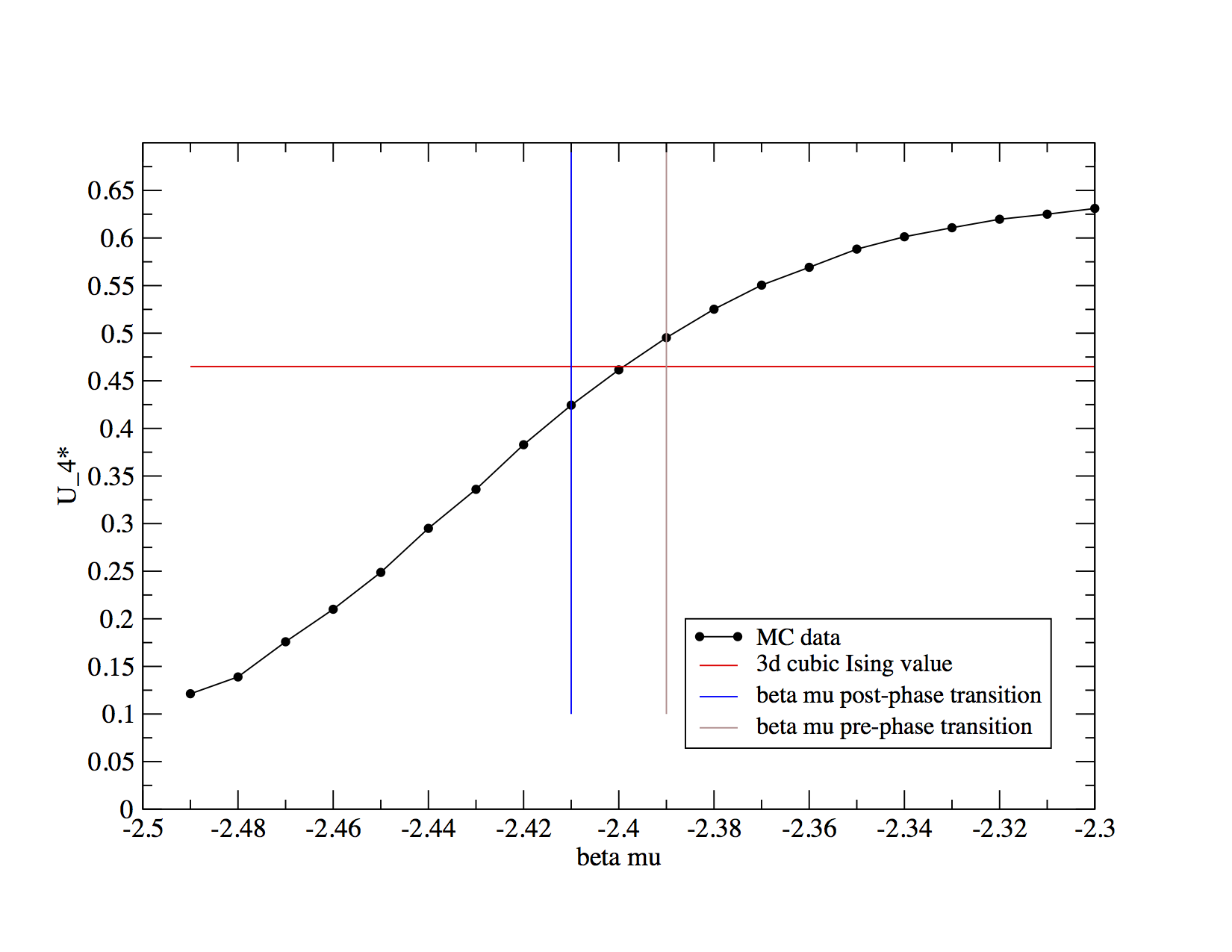
Figure 9: Binder cumulant $U_{4}^{*}$ as a function $\beta\mu$ for $J=0.675k_{B}T$, $\epsilon=2.55k_{B}T$, and $\epsilon^{\prime}=1k_{B}T$. The horizontal dashed line represents the three-dimensional cubic Ising universality value of 0.465 The horizontal red line indicates the universal value $U_{4}^{*}=0.465$ corresponding to the three-dimensional Ising model on a cubic lattice. Vertical lines bracket the range of $\beta\mu$ over which $F(\Delta n)$ changes convexity.

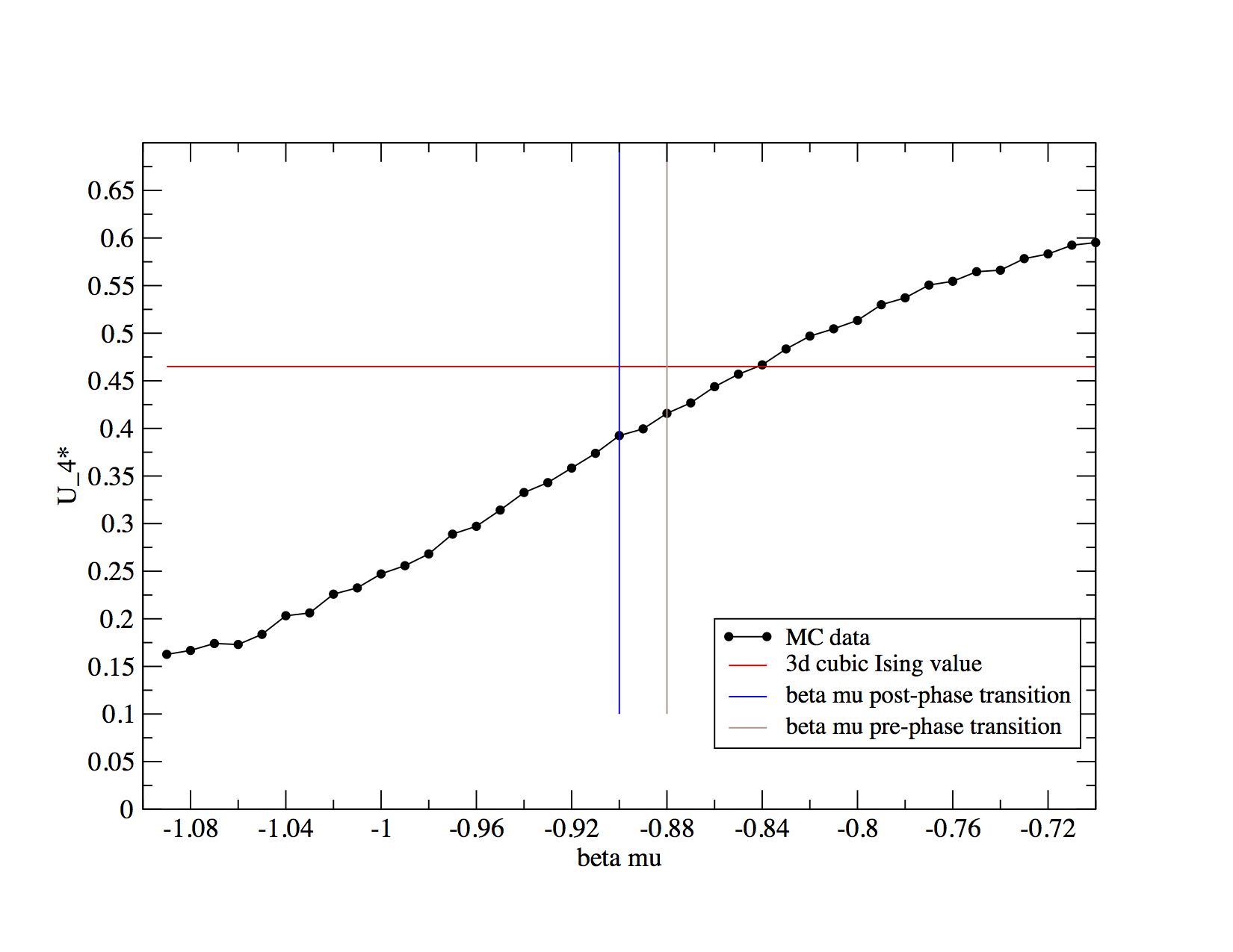
Figure 10: Binder cumulants for $\beta\mu$ at and near transition for $J=0.45k_{B}T$, $\epsilon=1.7k_{B}T$, and $\epsilon^{\prime}=20k_{B}T$. The horizontal dashed line represents the three-dimensional cubic Ising universality value of 0.465. Vertical lines bracket the range of $\beta\mu$ over which $F(\Delta n)$ changes convexity.

XI.3 Evidence for first-order transitions in simulation

Statistics of the order parameters $\Delta n$ and $\bar{n}$ can be obtained efficiently by routine umbrella sampling only for interaction strengths below $K\approx 6$. In this range we observe only continuous ordering in the thylakoid model. In order to evaluate the mean-field prediction of first-order transitions at high $K$, we employed a flat histogram sampling method analogous to Ref. Wang (2000). Adaptive biasing was applied to a variable $p_{11}$ that couples strongly to the high-density transition. Specifically,

$$p_{11}=\frac{2}{L_{x}L_{y}L_{z}}\sum_{z,i}n^{z}_{1,i}n^{z}_{2,i}$$

quantifies the instantaneous steric repulsion due to protein occupancy on both sides of a thylakoid disc. These simulations were performed by PLG.

Results of this flat histogram sampling are shown in Fig. 11 for systems with $L_{x}=L_{y}=6$ and $L_{z}=12$ at three different high values of $K$, and $\beta\epsilon^{\prime}=5.5$. Scaled log probabilities are shown for the global order parameters $\Delta n$, $\bar{n}$, and $p_{11}$ (top panels), and also for their disc-wise analogs (bottom panels), e.g.,

$$\bar{n}^{(\rm individual)}=\frac{1}{L_{x}L_{y}}\sum_{\alpha,i}n^{z}_{\alpha,i},$$

where $z$ could refer to any of the discs. (Because discs are statistically equivalent, we accumulate statistics over all values of $z$.) The index $s$ specifies one of these six order parameters. For each $s$, the corresponding scaling factor $N_{s}$ is chosen so that the plotted quantities serve as large deviation rate functions: For $\bar{n}$, $N_{s}=L_{x}L_{y}L_{z}$; for $\Delta n$, $N_{s}=L_{x}L_{y}L_{z}/2$; and for $p_{11}$, $N_{s}=L_{x}L_{y}L_{z}/2$. For the disc-wise analogs, $N_{s}=L_{x}L_{y}$ in each case.

For each $K$, we consider a value of $\mu$ that is very close to the high-density phase boundary, namely $\beta\mu=2.8$ for $K=5$, $\beta\mu=2.4$ for $K=6$, and $\beta\mu=1.93$ for $K=7$.

For $K=5$, computed distributions are consistent with results of umbrella sampling described in the main text. Fluctuations of $\Delta n$ are extremely broad at the transition, and distributions of the remaining order parameters show no exceptional features.

By contrast, for $K=7$ we observe several features that point towards discontinuous ordering. Distributions of extensive parameters acquire considerable structure, suggesting stiff horizontal domain boundaries that span the lateral dimensions of a disc. In this scenario, appropriate alternation of coexisting striped and doubly occupied discs can yield very low interfacial free energy, favoring a handful of specific order parameter values. This same structure, however, complicates the identification of bistability characteristic of a first-order transition. Such bistability is instead apparent in the disc-wise statistics, which are clearly bimodal.

In the intermediate case $K=6$, the statistics of these parameters show hints of emerging bistability. At the ordering transition each distribution exhibits fat tails, but none features distinct bimodality. We therefore estimate the onset of discontinuous ordering somewhere in the range $6<K<7$.

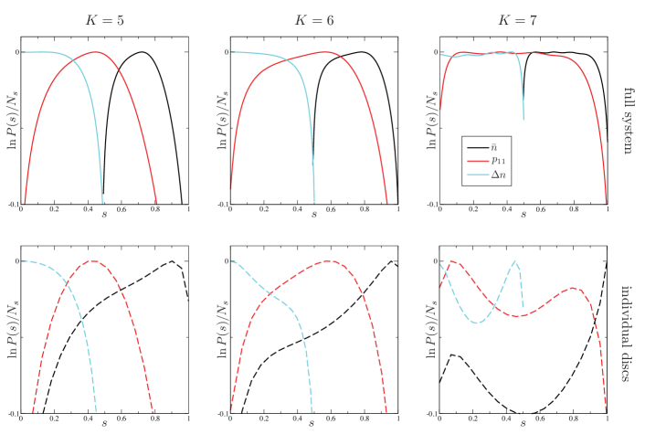
Figure 11: Log probability distributions for order parameters $\bar{n}$, $\Delta n$, and $p_{11}$ (top row), as well as their disc-wise analogs (bottom row). Fat tails at the ordering transition develop as $K$ is increased (moving from left to right in the figure columns). Clear multiple peaks at large $K$ strongly suggest the macroscopic bimodality underlying discontinuous phase transitions.

XII Methods and Results: Mean-field theory

Mean-field phase diagrams were obtained by numerically minimizing the free energy in Eq. (5) or (6) of the main text. We found it most efficient to do so by iterating self-consistent equations that determine local free energy minima. Here we provide these self-consistent equations, which result from differentiating $F_{\rm MF}$, and detail other aspects of our mean-field analysis.

XII.0.1 Self-consistent equations for the hard constraint limit

The hard constraint MFT average order parameter is

$$\Delta n=\frac{1}{2}\frac{e^{\beta\mu}(e^{K\bar{n}^{(1)}}-e^{K\bar{n}^{(2)}})}{1+e^{\beta\mu}e^{K\bar{n}^{(1)}}+e^{\beta\mu}e^{K\bar{n}^{(2)}}}$$ (12)

where $\bar{n}^{(i)}$ refers to the average density in the $i$th layer. Mutatis mutandis for $\bar{n}^{(2)}$. The average density is

$$\bar{n}=\frac{1}{2}\frac{e^{\beta\mu}(e^{K\bar{n}^{(1)}}+e^{K\bar{n}^{(2)}})}{1+e^{\beta\mu}e^{K\bar{n}^{(1)}}+e^{\beta\mu}e^{K\bar{n}^{(2)}}}$$ (13)

XII.1 Onset of first-order transitions for the hard constraint limit

We identify the onset of discontinuous transitions by posing the question: As the free energy extremum at $\bar{n}=1/K$ and $\Delta n=0$ loses local stability, do lower-lying minima of $F_{\rm MF}$ exist? Near the onset we assume that such minima reside at very small $\Delta n$ and at $\bar{n}$ very close to $1/K$; for a given value of $\bar{n}$, these minima $\Delta n^{*}$ satisfy

$$\centering\Delta n^{*2}=3\bar{n}^{3}\bigg{(}K-\frac{1}{\bar{n}}\bigg{)}\@add@centering$$ (14)

where we have neglected terms of order $\Delta n^{4}$.

Setting $\bar{n}=1/K+\eta$, Eq. 14 gives

$$\centering\Delta n^{*}=\pm\sqrt{\frac{3}{K}\eta}+O(\eta^{3/2})\@add@centering$$ (15)

To lowest order in $\eta$, the mean-field free energy $F_{\rm MF}(\bar{n},\Delta n)$ at the putative satellite minima can then be written

$$\centering\frac{2\beta}{N}F_{\rm MF}\bigg{(}1/K+\eta,\pm\sqrt{\frac{3}{K}\eta}\bigg{)}\@add@centering =\frac{2\beta}{N}F_{\rm MF}\bigg{(}1/K,0\bigg{)}$$

$$+\bigg{(}-3K+\frac{4K}{K-2}\bigg{)}\eta^{2}$$ (16)

For $K>10/3$, this free energy lies below that of the critical state at $\bar{n}=1/K$ and $\Delta n=0$. In other words, symmetry breaking occurs discontinuously, before the symmetric state becomes permissive of macroscopic fluctuations.

XII.2 Self-consistent equations for soft steric repulsion

Minimizing the free energy Eq. (7) with respect to $p_{10}$, $p_{01}$, $p_{11}$, and $p_{00}=1-(p_{10}+p_{01}+p_{11})$ gives nonlinear expressions for the mean density in alternating layers,

$$n_{1}=p_{10}+p_{11}=\frac{1}{q}(ae^{Kn_{1}}+\delta a^{2}e^{K(n_{1}+n_{2})}),$$ (17)

and

$$n_{2}=p_{01}+p_{11}=\frac{1}{q}(ae^{Kn_{2}}+\delta a^{2}e^{K(n_{1}+n_{2})}),$$ (18)

where $a=e^{\beta\mu}$, $\delta=e^{-\beta\epsilon^{\prime}}$, and

$$q=1+a(e^{Kn_{1}}+e^{Kn_{2}})+\delta a^{2}e^{K(n_{1}+n_{2})}.$$ (19)

Iteration of these expressions converges rapidly to local minima of $F_{\rm MF}$. From these solutions, our primary order parameters are computed simply from $\bar{n}=(n_{1}+n_{2})/2$, and $\Delta n=(n_{1}-n_{2})/2$.

XII.3 Continuous transitions for soft steric repulsion

For finite $\epsilon^{\prime}$, the extremum of $F_{\rm MF}$ at $\Delta n=0$ becomes locally unstable when

$$\bar{n}=\frac{1}{2}\pm\frac{1}{2K}\sqrt{(K-2)^{2}-4\delta},$$ (20)

defining possible continuous transitions in the $(K,\bar{n})$ plane. Fig. 12 shows both lines of solutions in the $(K,\beta\mu)$ plane, for several values of $\epsilon^{\prime}$. In each case the two lines cross at an attraction strength $K_{\rm cross}(\epsilon^{\prime})$. For $\beta\epsilon^{\prime}\geq 2$, $K_{\rm cross}$ lies outside the range of this plot.

Continuous transitions predicted for $K>K_{\rm cross}$ violate a fundamental thermodynamic requirement of stability. Specifically, the solution with higher density $\bar{n}$ occurs at a lower chemical potential than the low-density solution, implying a negative compressibility. Although these solutions represent local free energy minima, they cannot be global minima. Indeed, numerical minimization of $F_{\rm MF}$ identifies lower-lying minima in all cases.

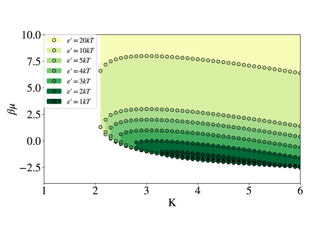
Figure 12: Soft constraint model $\beta\mu$ vs. $K$ phase diagram, continuous mean-field transitions according to Eq. (20). Shaded region indicates the striped phase.

XII.4 Self-consistent equations for soft steric repulsion

Minimizing the mean-field free energy for finite $\epsilon^{\prime}$ yields nonlinear equations for the average layer densities:

$$\langle n_{i}\rangle=\frac{1}{q}(ae^{Kn_{i}}+\delta a^{2}e^{2Kn}),$$ (21)

In terms of $n$ and $\Delta n$,

$$n=\frac{1}{2q}\bigg{[}ae^{Kn}(e^{K\Delta n}+e^{-K\Delta n})+2a^{2}e^{2Kn}\delta\bigg{]}$$ (22)

$$\Delta n=\frac{1}{2q}\bigg{[}ae^{Kn}(e^{K\Delta n}-e^{-K\Delta n})\bigg{]}$$ (23)

where $a=e^{\beta\mu}$, $\delta=e^{-\beta\epsilon^{\prime}}$, $n=\frac{1}{2}(n_{1}+n_{2})$, and $\Delta n=\frac{1}{2}(n_{1}-n_{2})$.

XII.5 Solving self-consistent equations

Iterating the self-consistent equations (22) and (23) converges readily to local extrema of the mean-field free energy. After $10^{6}$ steps, additional iteration changes values of $n_{1}$ and $n_{2}$ by less than $10^{-12}$.

Under many conditions, however, this free energy surface exhibits three or more distinct minima. The end result of iteration thus depends on initial values of $n_{1}$ and $n_{2}$. We considered five different $(n_{1},n_{2})$ pairs, namely (0.6, 0.4), (0.1, 0.1), (0.9, 0.9), (0.9, 0.1), and (0.2, 0.1). For each set of conditions, we then select the self-consistent solution with lowest free energy.

A resulting value of $|n_{1}-n_{2}|$ greater than $10^{-9}$ was taken to signify thermodynamic stability of the ordered phase.

XIII Methods and Results: Bethe-Peierls approximation

XIII.1 One-cluster expressions

Our site cluster, depicted in Fig. 13, encompasses two thylakoid discs, so as to capture one instance of the striped motif in the striped phase.

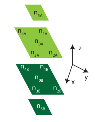
Figure 13: Bethe-Peierls cluster schematic. $n_{0X}$ is the central site, and all others are neighboring sites. Dark-colored sites denote sites in a densely populated stripe, and light-colored sites represent sites in a sparsely populated stripe.

The cluster Hamiltonian is

$$\centering H\@add@centering =-\mu(n_{0A}+n_{0B})-J\sum_{i=1}^{4}(n_{0A}n_{iA}+n_{0B}n_{iB})$$

$$-\epsilon(n_{0A}n_{5A}+n_{0B}n_{5B})+\epsilon^{\prime}n_{0A}n_{0B}$$

$$-\mu_{A}\sum_{i=1}^{4}n_{iA}-\mu_{B}\sum_{i=1}^{4}n_{iB}-\mu_{A}^{\prime}n_{5A}-\mu_{B}^{\prime}n_{5B}$$ (24)

where $A$ and $B$ denote different stripes.

In a BP ansatz, instead of solving for average densities, one solves for effective fields; these are given by $\mu_{A}$, $\mu_{B}$, $\mu_{A}^{\prime}$, and $\mu_{B}^{\prime}$. There are four fields because sites interfacing with a stripe of the opposite type experience a different field than those surrounded by like sites.

If we take $J=\epsilon$, then $\mu_{k}^{\prime}=\mu_{k}$. With this in mind, we write the partition function. First, below are some important variable assignments:

$$\mu_{A} =\bar{\mu}+\Delta\mu,\mu_{B}=\bar{\mu}-\Delta\mu$$

$$z =e^{\beta\mu},z_{A}=e^{\beta\mu_{A}},z_{B}=e^{\beta\mu_{B}}$$

$$\bar{z} =e^{\beta\bar{\mu}},\delta=e^{-\beta\epsilon^{\prime}},c=e^{K}$$

Taking the standard derivatives of Eq. (XIII.1), the average densities are Eq. (XIII.1) and its $n_{0B}$ counterpart. Note that there are two average densities for each stripe, with $n_{0x}$ as the central sites and the others its neighboring sites.

$$\centering Q\@add@centering =\sum_{n_{0A},n_{0B}}z^{n_{0A}+n_{0B}}\delta^{n_{0A}n_{0B}}\bigg{(}1+z_{A}e^{Kn_{0A}}\bigg{)}^{5}\bigg{(}1+z_{B}e^{Kn_{0B}}\bigg{)}^{5}$$

$$=\bigg{(}1+\bar{z}e^{\beta\Delta\mu}\bigg{)}^{5}\bigg{(}1+\bar{z}e^{-\beta\Delta\mu}\bigg{)}^{5}$$

$$+z\bigg{(}1+c\bar{z}e^{\beta\Delta\mu}\bigg{)}^{5}\bigg{(}1+\bar{z}e^{-\beta\Delta\mu}\bigg{)}^{5}$$

$$+z\bigg{(}1+\bar{z}e^{\beta\Delta\mu}\bigg{)}^{5}\bigg{(}1+c\bar{z}e^{-\beta\Delta\mu}\bigg{)}^{5}$$

$$+z^{2}\delta\bigg{(}1+c\bar{z}e^{\beta\Delta\mu}\bigg{)}^{5}\bigg{(}1+c\bar{z}e^{-\beta\Delta\mu}\bigg{)}^{5}$$ (25)

$$\langle n_{0A}\rangle =\frac{1}{Q}\bigg{(}1+c\bar{z}e^{\beta\Delta\mu}\bigg{)}^{5}z\bigg{[}\bigg{(}1+\bar{z}e^{-\beta\Delta\mu}\bigg{)}^{5}$$

$$+z\delta\bigg{(}1+c\bar{z}e^{-\beta\Delta\mu}\bigg{)}^{5}\bigg{]}$$ (26)

$$\langle n_{A}\rangle =\frac{1}{5Q}\frac{\partial Q}{\partial\beta\mu_{A}}=\frac{z_{A}}{5Q}\frac{\partial Q}{\partial z_{A}}$$

$$=\frac{\bar{z}e^{\beta\Delta\mu}}{Q}\bigg{\{}\bigg{(}1+\bar{z}e^{\beta\Delta\mu}\bigg{)}^{4}\bigg{[}\bigg{(}1+\bar{z}e^{-\beta\Delta\mu}\bigg{)}^{5}+z\bigg{(}1$$

$$+c\bar{z}e^{-\beta\Delta\mu}\bigg{)}^{5}\bigg{]}+cz\bigg{(}1+c\bar{z}e^{\beta\Delta\mu}\bigg{)}^{4}\bigg{[}\bigg{(}1+\bar{z}e^{-\beta\Delta\mu}\bigg{)}^{5}$$

$$+z\delta\bigg{(}1+c\bar{z}e^{-\beta\Delta\mu}\bigg{)}^{5}\bigg{]}\bigg{\}}$$ (27)

Here we have replaced $\mu_{A}$ and $\mu_{B}$ with $\bar{\mu}+\Delta\mu$ and $\bar{\mu}-\Delta\mu$, as this formulation more intuitively allows one to discuss the fields in terms of an average field and fluctuations from it. The astute reader will notice the factor of 5 in Eq. (XIII.1) – this is the number of nearest neighbors in the same lattice $A$. In general, this number would be $2d-1$, where $d$ is the total dimensionality of the system; other factors in Eq. (XIII.1) may change with different $d$. The difference between $\langle n_{iA}\rangle$ and $\langle n_{iB}\rangle$ simply involves replacing $\mu_{A}$ with $\mu_{B}$ and vice versa; for this reason, $\langle n_{iB}\rangle$ expressions are not shown here.

Since we have two unknowns, $\bar{\mu}$ and $\Delta\mu$, instead of solving one self-consistency expression as for mean field theory, one must solve a system of equations. The system is Eqs. (XIII.1) or  (XIII.1). The system was initialized for both small and large $\delta\mu$ and for initial $\mu_{i}$ large and small. The tolerance for self-consistency was $10^{-12}$, and the maximum number of iterations was 1 million. The transition was determined by finding $\Delta n$ differences larger than $10^{-9}$ between consecutive $\beta\mu$ values for a given $K$.

$$\langle n_{0A}\rangle =\langle n_{A}\rangle$$

$$\langle n_{0B}\rangle =\langle n_{B}\rangle$$ (28)

$$\langle\Delta n_{0}\rangle-\langle\Delta n\rangle =0$$

$$\langle\bar{n_{0}}\rangle+\langle\bar{n}\rangle =0$$ (29)

where $\Delta n_{i}=\frac{1}{2}(n_{A}-n_{B})$ and $\bar{n_{i}}=\frac{1}{2}(n_{A}+n_{B})$.

XIII.2 Phase diagrams

Here we present Bethe-Peierls phase diagrams, in both the $\beta\mu$ vs. $K$ and $\bar{n}$ vs. $K$ planes. Figs. 14 and 15 show a larger range of $K$ values than we presented for two-site mean field theories. Only at these larger values of $K$ are signs of discontinuous ordering apparent at the BP level of mean field theory.

Continuous BP transitions can be determined by linearizing the self-consistent equations. The resulting equations, which are polynomial in $\bar{z}$, are amenable to numerical root finding methods. Continuous transitions can also be located by initializing the nonlinear self-consistent iteration appropriately. These continuous transitions, plotted in Figs. 15 and 17 (on different scales), show the same unphysical crossing behavior found with the two-site approach, though this crossing occurs at a larger $K$ value than in the previous approach.

Self-consistent solutions obtained with a different initialization are plotted in Fig. 14 over a wide range of $K$. At small $K$ they coincide with the continuous transitions described above, as emphasized in Fig. 16, which shows only the range of $K$ accessible in simulations. Limited to the domain $1<K<6$, this plot is essentially identical to the continuous case Fig. 17. For large $K$, however, this initialization produces different solutions, which do not cross. Instead, these phase boundaries exhibit discontinuous change in both $\Delta n$ and $\bar{n}$, and widen markedly at high $K$. All of these features are consistent with results of two-site MF theory, but they set in at higher $K$. For the range of $\epsilon^{\prime}$ we have studied, the onset of first-order transitions occurs near $K=6$, as opposed to the two-site result of $K\approx 10/3$. As per the data of Sec. XI.3, first-order transitions are observed in simulation between $K=6$ and $K=7$, demonstrating that Bethe-Peierls does indeed more accurately estimate the location of discontinuous transitions in this model.

The minimum value of $K$ at which ordering occurs is also shifted upwards in BP theory, to about $K=2.4$. This prediction compares more favorably with the critical value $K\approx 2.7$ found in simulations than does the two-site prediction $K\approx 2$.

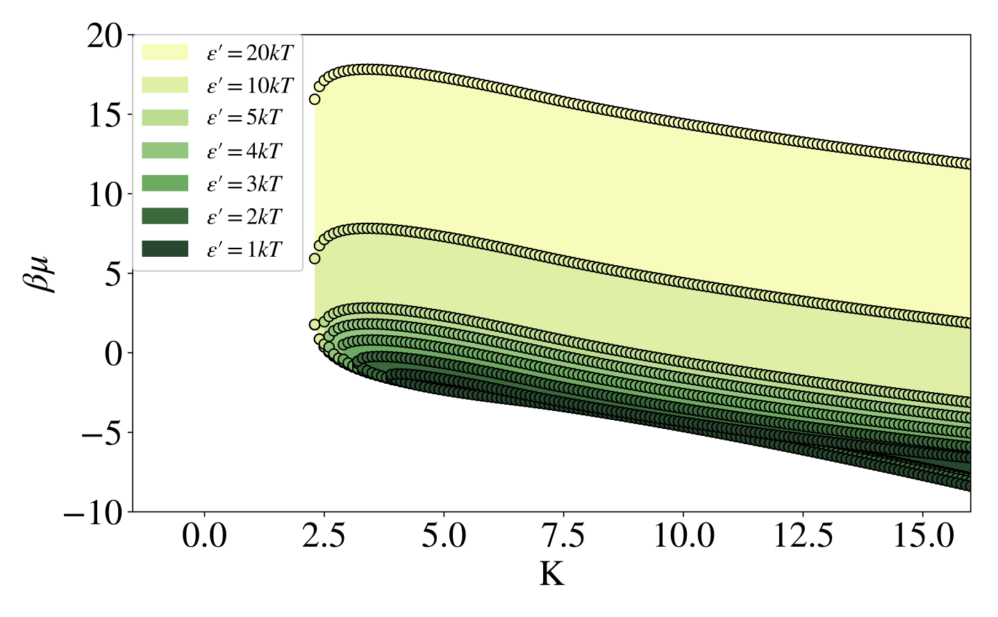
Figure 14: BP $\beta\mu$ vs. $K$ phase diagram, with first-order transitions beginning $K\approx 6$. Shaded region indicates the striped phase. The upper branch was calculated via the inversion symmetry relation Eq. (4) in the main text.

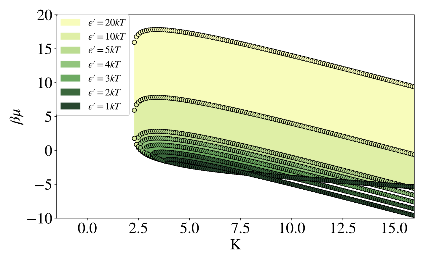
Figure 15: BP $\beta\mu$ vs. $K$ phase diagram, continuous transitions throughout. Shaded region indicates the striped phase. The upper branch was calculated via the inversion symmetry relation Eq. (4) in the main text.

Again, viewed on the same scale as results in the main text, the BP data very strongly resemble the results of two-site mean field theory; see Figs. 16 to 17. Note that these two figures are essentially identical as the discontinuous transitions begin at $K\approx 6$.

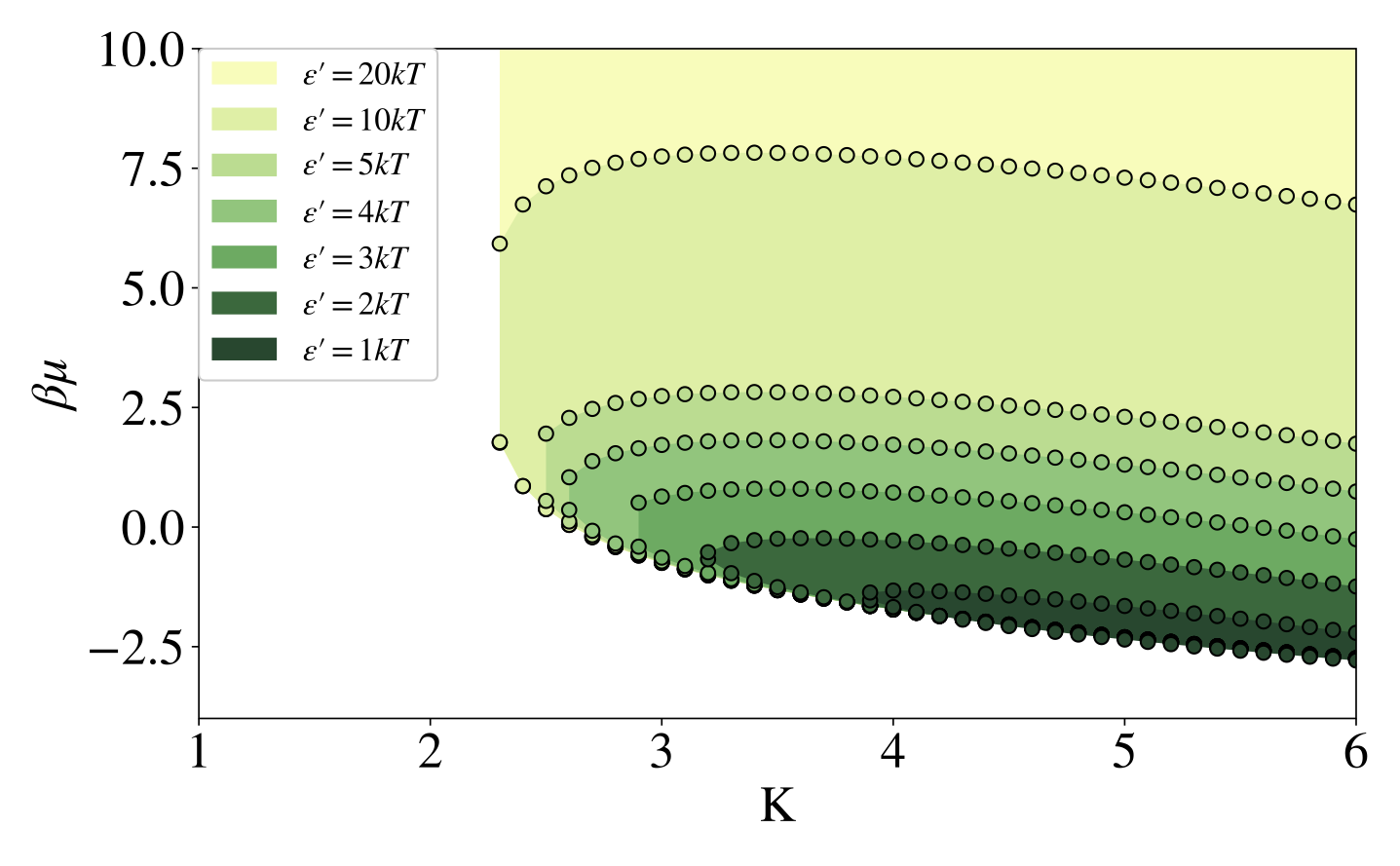
Figure 16: BP $\beta\mu$ vs. $K$ phase diagram, with first-order transitions beginning $K\approx 6$ (not visible here). Shaded region indicates the striped phase. The upper branch was calculated via Eq. (4) in the main text.

Figure 17: BP $\beta\mu$ vs. $K$ phase diagram, continuous transitions throughout. Shaded region indicates the striped phase. The upper branch was calculated via Eq. (4) in the main text.

XIII.3 Two-cluster Bethe-Peierls approximation

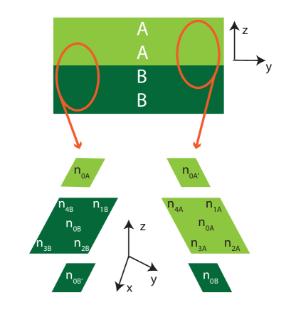
Figure 18: Two-cluster schematic. The top bar represents four layers, with two sets of two-layer stripes. The lower half of the diagram represents the clusters used in the BP approximation, with $n_{0x}$ as the centers of the clusters.

As mentioned in the main text, another way to account for alternating couplings in a lattice model using BP is to use two clusters instead of one (see Fig. 18). One cluster corresponds to a sparsely populated stripe, and the other a densely populated stripe. To start, we write the cluster Hamiltonian for cluster $A$:

$$\begin{split}H_{A}&=-\mu n_{0A}-\mu_{B}n_{0B}-Jn_{0A}(n_{1A}+n_{2A}+n_{3A}+n_{4A})\\ &-\mu_{A}(n_{1A}+n_{2A}+n_{3A}+n_{4A}+n_{0A^{\prime}})\\ &+\epsilon^{{}^{\prime}}n_{0A}n_{0B}-\epsilon n_{0A}n_{0A^{\prime}}\end{split}$$ (30)

The cluster Hamiltonian for the $B$ lattice can be obtained similarly. The average densities arise in the traditional way, via derivatives of the partition function:

$$\langle n_{0A}\rangle =\frac{\partial\ln Z_{A}}{\partial\beta\mu}=\frac{1}{Z_{A}}e^{\beta\mu}\bigg{(}1+e^{\beta(\bar{\mu}+\Delta\mu+J)}\bigg{)}^{4}$$ (31)

$$\times\bigg{(}1+e^{\beta(\bar{\mu}-\Delta\mu-\epsilon^{{}^{\prime}})}\bigg{)}\bigg{(}1+e^{\beta(\bar{\mu}+\Delta\mu+\epsilon)}\bigg{)}$$

$$\langle n_{A}\rangle =\frac{1}{5}\frac{\partial\ln Z_{A}}{\partial\beta\mu_{A}}$$ (32)

$$=\frac{1}{5Z_{A}}\bigg{[}5\bigg{(}1+e^{\beta(\bar{\mu}+\Delta\mu})\bigg{)}^{4}e^{\beta(\bar{\mu}+\Delta\mu)}\bigg{(}1+e^{\beta(\bar{\mu}-\Delta\mu)}\bigg{)}$$

$$+4\bigg{(}1+e^{\beta(\bar{\mu}+\Delta\mu+J)}\bigg{)}^{3}e^{\beta(\bar{\mu}+\Delta\mu+J)}e^{\beta\mu}\bigg{(}1+e^{\beta(\bar{\mu}-\Delta\mu-\epsilon^{{}^{\prime}})}\bigg{)}\bigg{(}1+e^{\beta(\bar{\mu}+\Delta\mu+\epsilon)}\bigg{)}$$

$$+e^{\beta\mu}e^{\beta(\bar{\mu}+\Delta\mu+\epsilon)}\bigg{(}1+e^{\beta(\bar{\mu}-\Delta\mu-\epsilon^{{}^{\prime}})}\bigg{)}\bigg{(}1+e^{\beta(\bar{\mu}+\Delta\mu+J)}\bigg{)}^{4}\bigg{]}$$

Using these expressions, the same systems of equations  (XIII.1) or (XIII.1) were solved via gradient descent optimization to find continuous transitions. Please note that no first-order transitions were found for this model, and nor did these equations preserve occupation inversion symmetry.

XIII.3.1 Momentum-boosted gradient descent

The system of equations, Eq. (XIII.1), was rephrased as a root-finding problem in Eq. (XIII.1), such that a gradient descent method could be used to find its roots. Consequently, one can imagine the system of equations as a vector whose components are the equations. Thus, the objective function optimized was the magnitude of this vector – namely, the sum of the squared equations set equal to zero.

A gradient descent approach was used for a number of reasons. Firstly, the ideal initial conditions for this system were unknown, so a method that can handle initial conditions far from the solution was desired; many root-finding and optimization algorithms do not do well when seeded far from the solution. Second, so as to handle potentially multiple solutions for a given set of parameters, we wanted a method that had the ability to find multiple minima – this concern is related to the first, since initial conditions must be given differently so as to explore possible multiple global solutions. Gradient descent is algorithmically simple and has mostly guaranteed convergence, hence it was chosen.

Furthermore, MGD was utilized instead of plain steepest descent as a means of increasing efficiency and preventing traps in local optima. Ruder (2017) One can write the $x$ component of the update vector at the next step as

$$v_{x,t+1} =\gamma v_{x,t}+s\nabla_{x}f$$

$$x =x-v_{x,t+1}$$ (33)

where $\gamma$ is the momentum scalar that usually is between 0.9 and 1 and encodes the ”memory” of the previous step, and $s$ is the step size for the descent. The step size is on the order of 0.1 to 0.0001 usually. Convergence was determined by how close both the objective function and the gradient were to zero. The gradient of Eq. (XIII.1) was approximated using finite differences.

For each system of BP equations, the initial conditions were generated by creating a grid of ($\Delta\mu$, $\bar{\mu}$) values. Since $\bar{\mu}$ was expected to remain relatively close to $\mu$, a limited number of $\bar{\mu}$ initial guesses were used. For $\Delta\mu$, a grid ranging from -2 to 2 $k_{B}T$ measured out by a given increment were used; based on preliminary explorations, solutions obeying the constraints of the problem are only found for relatively small $\Delta\mu$ (that is, $\Delta\mu$ within these bounds).

References

- Dekker and Boekema (2005) J. P. Dekker and E. J. Boekema, “Supramolecular organization of thylakoid membrane proteins in green plants,” Biochim. Biophys. Acta 1706, 12–39 (2005).
- Pribil, Labs, and Leister (2014) M. Pribil, M. Labs, and D. Leister, “Structure and dynamics of thylakoids in land plants,” J. Exp. Bot. 65, 1955–1972 (2014).
- Nevo et al. (2012) R. Nevo, D. Charuvi, O. Tsabari, and Z. Reich, “Composition, architecture, and dynamics of the photosynthetic apparatus in higher plants,” Plant J. 70, 157–176 (2012).
- Daum and Kühlbrandt (2011) B. Daum and W. Kühlbrandt, “Electron tomography of plant thylakoid membranes,” J. Exp. Bot. 62, 2393–2402 (2011).
- Qin et al. (2015) X. Qin, M. Suga, T. Kuang, and J. Shen, “Structural basis for energy transfer pathways in the plant PSI-LHCI supercomplex,” Science 348, 989–995 (2015).
- Wei et al. (2016) X. Wei, X. Su, P. Cao, X. Liu, W. Chang, M. Li, X. Zhang, and Z. Liu, “Structure of spinach photosystem II-LHCII supercomplex at 3.2 Å resolution,” Nature 534, 69–74 (2016).
- Liguori et al. (2015) N. Liguori, X. Periole, S. J. Marrink, and R. Croce, “From light-harvesting to photoprotection: structural basis of the dynamic switch of the major antenna complex of plants (LHCII),” Sci. Rep. 5 (2015), 10.1038/srep15661.
- Nosek et al. (2017) L. Nosek, D. Semchonok, E. J. Boekema, P. Ilík, and R. Kouřil, “Structural variability of plant photosystem II megacomplexes in thylakoid membranes,” Plant J. 89, 104–111 (2017).
- Schneider and Geissler (2013) A. R. Schneider and P. L. Geissler, “Coexistence of fluid and crystalline phases of proteins in photosynthetic membranes,” Biophys. J 105, 1161–1170 (2013).
- Chow et al. (2005) W. S. Chow, E. Kim, P. Horton, and J. M. Anderson, “Granal stacking of thylakoid membranes in higher plant chloroplasts: the physicochemical forces at work and the functional consequences that ensue,” Photochem. Photobiol. Sci. 4, 1081–1090 (2005).
- Kirchhoff et al. (2007a) H. Kirchhoff, W. Haase, S. Haferkamp, T. Schott, M. Borinski, U. Kubitscheck, and M. Rögner, “Structural and functional self-organization of photosystem II in grana thylakoids,” Biochim. Biophys. Acta 1767, 1180–1188 (2007a).
- Standfuss et al. (2005) J. Standfuss, A. C. Terwisscha van Scheltinga, M. Lamborghini, and W. Kuhlbrandt, “Mechanisms of photoprotection and nonphotochemical quenching in pea light-harvesting complex at 2.5 Å resolution,” EMBO J. 24, 919–928 (2005).
- Phuthong et al. (2015) W. Phuthong, Z. Huang, T. M. Wittkopp, K. Sznee, M. L. Heinnickel, J. P. Dekker, R. N. Frese, F. B. Prinz, and A. R. Grossman, “The use of contact mode atomic force microscopy in aqueous medium for structural analysis of spinach photosynthetic complexes,” Plant Physiol. 169, 1318–1332 (2015).
- Onoa et al. (2014) B. Onoa, A. R. Schneider, M. D. Brooks, P. Grob, E. Nogales, P. L. Geissler, K. K. Niyogi, and C. Bustamante, “Atomic force microscopy of photosystem II and its unit cell clustering quantitatively delineate the mesoscale variability in Arabidopsis thylakoids,” PLOS ONE 9 (2014), 10.1371/journal.pone.0101470.
- Ruban and Johnson (2015) A. V. Ruban and M. P. Johnson, “Visualizing the dynamic structure of the plant photosynthetic membrane,” Nat. Plants 1 (2015), 10.1038/NPLANTS.2015.161.
- Schneider and Geissler (2014) A. R. Schneider and P. L. Geissler, “Coarse-grained computer simulation of dynamics in thylakoid membranes: methods and opportunities,” Front. Plant Sci. 4 (2014), 10.3389/fpls.2013.00555.
- Lee, Pao, and Smit (2015) C. Lee, C. Pao, and B. Smit, “PSII-LHCII supercomplex organizations in photosynthetic membrane by coarse-grained simulation,” J. Phys. Chem. B 119, 3999–4008 (2015).
- Amarnath et al. (2016) K. Amarnath, D. I. G. Bennett, A. R. Schneider, and G. R. Fleming, “Multiscale model of light harvesting by photosystem II in plants,” Proc. Nat. Acad. Sci. 113, 1156–1161 (2016).
- Erickson, Wakao, and Niyogi (2015) E. Erickson, S. Wakao, and K. K. Niyogi, “Light stress and photoprotection in Chlamydomonas reinhardtii,” Plant J. 82, 449–465 (2015).
- Kirchhoff et al. (2011) H. Kirchhoff, C. Halla, M. Wood, M. Herbstová, O. Tsabarib, R. Nevob, D. Charuvib, E. Shimonic, and Z. Reich, “Dynamic control of protein diffusion within the granal thylakoid lumen,” Proc. Nat. Acad. Sci. 108, 20248–20253 (2011).
- Kirchhoff (2014) H. Kirchhoff, “Diffusion of molecules and macromolecules in thylakoid membranes,” Biochim. Biophys. Acta, Bioenerg. 1837, 495–502 (2014).
- Albertsson (1982) P.-r. Albertsson, “Interaction between the lumenal sides of the thylakoid membrane,” FEBS Lett. 149, 186–190 (1982).
- Puthiyaveetil, van Oort, and Kirchhoff (2017) S. Puthiyaveetil, B. van Oort, and H. Kirchhoff, “Surface charge dynamics in photosynthetic membranes and the structural consequences,” Nat. Plants 3, 17020 (2017).
- Capretti et al. (2019) A. Capretti, A. K. Ringsmuth, J. F. van Velzen, A. Rosnik, R. Croce, and T. Gregorkiewicz, “Nanophotonics of higher-plant photosynthetic membranes,” Light: Sci. Appl. 8 (2019), 10.1038/s41377-018-0116-8.
- Speck, Reister, and Seifert (2010) T. Speck, E. Reister, and U. Seifert, “Specific adhesion of membranes: Mapping to an effective bond lattice gas,” Phys. Rev. E 82, 021923 (2010).
- Machta, Veatch, and Sethna (2012) B. B. Machta, S. L. Veatch, and J. P. Sethna, “Critical Casimir forces in cellular membranes,” Phys. Rev. Lett. 109, 1–5 (2012).
- Naji and Brown (2007) A. Naji and F. L. H. Brown, “Membrane-protein interactions in a generic coarse-grained model for lipid bilayers,” J. Chem. Phys. 126, 235103 (2007).
- Schick (2012) M. Schick, “Membrane heterogeneity: Manifestation of a curvature-induced microemulsion,” Phys. Rev. E 85, 031902 (2012).
- Garbès Putzel and Schick (2012) G. Garbès Putzel and M. Schick, “Phase behavior of a model bilayer membrane with coupled leaves,” Biophys. J. 94, 869–877 (2012).
- Frazier et al. (2007) M. L. Frazier, J. R. Wright, A. Pokorny, and P. F. F. Almeida, “Investigation of domain formation in sphingomyelin/cholesterol/POPC mixtures by fluorescence resonance energy transfer and Monte Carlo simulations,” Biophys. J 92, 2422–2433 (2007).
- Yethiraj and Weisshaar (2007) A. Yethiraj and J. Weisshaar, “Why are lipid rafts not observed in vivo?” Biophys. J 93, 3113–3119 (2007).
- Honerkamp-Smith et al. (2008) A. Honerkamp-Smith, P. Cicuta, M. Collins, S. Veatch, M. den Nijs, M. Schick, and S. Keller, “Line tensions, correlation lengths, and critical exponents in lipid membranes near critical points,” Biophys. J 95, 236–246 (2008).
- Machta et al. (2011) B. Machta, S. Papanikolaou, J. Sethna, and S. Veatch, “Minimal model of plasma membrane heterogeneity requires coupling cortical actin to criticality,” Biophys. J 100, 1668–1677 (2011).
- Mitra et al. (2018) E. Mitra, S. Whitehead, D. Holowka, B. Baird, and J. Sethna, “Computation of a theoretical membrane phase diagram and the role of phase in lipid-raft-mediated protein organization,” J. Phys. Chem. B 122, 3500–3513 (2018).
- Meerschaert and Kelly (2015) R. Meerschaert and C. Kelly, “Trace membrane additives affect lipid phases with distinct mechanisms: a modified ising model,” Eur. Biophys. J 44, 227–233 (2015).
- Hoshino, Komura, and Andelman (2015) T. Hoshino, S. Komura, and D. Andelman, “Correlated lateral phase separations in stacks of lipid membranes,” J. Chem. Phys. 143, 243124 (2015).
- Hoshino, Komura, and Andelman (2017) T. Hoshino, S. Komura, and D. Andelman, “Permeation through a lamellar stack of lipid mixtures,” EPL 120 (2017), 10.1209/0295-5075/120/18004.
- Tayebi et al. (2012) L. Tayebi, Y. Ma, D. Vashaee, G. Chen, S. K. Sinha, and A. N. Parikh, “Long-range interlayer alignment of intralayer domains in stacked lipid bilayers,” Nat. Mat. 11, 1074–1080 (2012).
- Tayebi, Parikh, and Vashaee (2013) L. Tayebi, A. N. Parikh, and D. Vashaee, “Long-range interlayer alignment of intralayer domains in stacked lipid bilayers,” Int. J. Mol. Sci. 14, 3824–3833 (2013).
- Ellis, Otto, and Touchette (2005) R. S. Ellis, P. T. Otto, and H. Touchette, “Analysis of phase transitions in the mean-field Blume-Emery-Griffiths model,” Ann. Appl. Probab. 15, 2203–2254 (2005).
- Deserno (1997) M. Deserno, “Tricriticality and the Blume-Capel model: A Monte Carlo study within the microcanonical ensemble,” Phys. Rev. E 56, 5204–5210 (1997).
- Ez-Zahraouy and Kassou-Ou-Ali (2004) H. Ez-Zahraouy and A. Kassou-Ou-Ali, “Phase diagrams of the spin-1 Blume-Capel film with an alternating crystal field,” Phys. Rev. B 69 (2004), 10.1103/PhysRevB.69.064415.
- Fisher and Selke (1980) M. E. Fisher and W. Selke, “Infinitely many commensurate phases in a simple Ising model,” Phys. Rev. Lett. 44, 1502–1505 (1980).
- Wu (1982) F. Y. Wu, “The Potts model,” Rev. Mod. Phys. 54, 235–267 (1982).
- Jho et al. (2011) Y. S. Jho, R. Brewster, S. A. Safran, and P. A. Pincus, “Long-range interaction between heterogeneously charged membranes,” Langmuir 27, 4439–4446 (2011).
- West, Brown, and Schmid (2009) B. West, F. L. H. Brown, and F. Schmid, “Membrane-protein interactions in a generic coarse-grained model for lipid bilayers,” Biophys. J. 96, 101–115 (2009).
- Meilhac and Destainville (2011) N. Meilhac and N. Destainville, “Clusters of proteins in biomembranes: Insights into the roles of interaction potential shapes and of protein diversity,” J. Phys. Chem. B 115, 7190–7199 (2011).
- Pasqua et al. (2010) A. Pasqua, L. Maibaum, G. Oster, D. A. Fletcher, and P. L. Geissler, “Large-scale simulations of fluctuating biological membranes,” J. Chem. Phys. 132, 1–6 (2010).
- Stachowiak et al. (2012) J. C. Stachowiak, E. M. Schmid, C. J. Ryan, H. S. Ann, D. Y. Sasaki, M. B. Sherman, P. L. Geissler, D. A. Fletcher, and C. C. Hayden, “Membrane bending by protein-protein crowding,” Nat. Cell Biol. 14, 944–949 (2012).
- Schmid et al. (2016) E. M. Schmid, M. H. Bakalar, C. Kaushik, J. Weichsel, H. S. Ann, P. L. Geissler, M. L. Dustin, and D. A. Fletcher, “Size-dependent protein segregation at membrane interfaces,” Nat. Phys. 12, 704–711 (2016).
- Heimburg (2007) T. Heimburg, Thermal biophysics of membranes (Weinheim: Wiley-VCH Verlag GmbH and Co., Weinheim, Germany, 2007).
- Fair (1965) G. Fair, “Bethe-Peierls-Weiss approximation and a model for ferromagnetic thin films,” Tech. Rep. D-2979 (National Aeronautics and Space Administration, Cleveland, Ohio, 1965).
- Neto, dos Anjos, and de Sousa (2006) M. A. Neto, R. A. dos Anjos, and J. R. de Sousa, “Anisotropic Ising model in a magnetic field: Effective-field theory analysis,” Phys. Rev. E 73 (2006), 10.1103/PhysRevB.73.214439.
- Schneider (2013) A. R. Schneider, Pattern formation in photosynthetic membranes: a physical and statistical approach, Ph.D. thesis, University of California-Berkeley (2013).
- Daum et al. (2010) B. Daum, D. Nicastro, J. Austin, J. McIntosh, and W. Kühlbrandt, “Arrangement of photosystem II and ATP synthase in chloroplast membranes of spinach and pea,” Plant Cell 22, 1299–1312 (2010).
- Nield et al. (2000) J. Nield, E. Orlova, E. Morris, B. Gowen, M. van Heel, and J. Barber, “3D map of the plant photosystem II supercomplex obtained by cryoelectron microscopy and single particle analysis,” Nat. Struct. Biol. 7, 44–47 (2000).
- Boekema et al. (2000) E. Boekema, J. van Breemen, H. van Roon, and J. Dekker, “Arrangement of photosystem II supercomplexes in crystalline macrodomains within the thylakoid membrane of green plant chloroplasts,” J. Mol. Biol. 301, 1123–1133 (2000).
- Jansson et al. (1997) S. Jansson, H. Stefánsson, U. Nyström, P. Gustafsson, and P.-r. Albertsson, “Antenna protein composition of PSI and PSII in thylakoid sub-domains,” Biochim. Biophys. Acta - Bioenergetics 1320, 297–309 (1997).
- Veerman et al. (2007) J. Veerman, M. McConnell, S. Vasilév, F. Mamedov, S. Styring, and D. Bruce, “Functional heterogeneity of photosystem II in domain specific regions of the thylakoid membrane of Spinach (Spinacia Oleracea L),” Biochem. 46, 3443–3453 (2007).
- Kirchhoff et al. (2007b) H. Kirchhoff, W. Haase, S. Wegner, R. Danielsson, R. Ackermann, and P.-r. Albertsson, “Low-light-induced formation of semicrystalline photosystem II arrays in higher plant chloroplasts,” Biochem. 46, 11169–11176 (2007b).
- Murphy (1986) D. Murphy, “The molecular organisation of the photosynthetic membranes of higher plants,” Biochim. Biophys. Acta 864, 33–94 (1986).
- Kirchhoff et al. (1986) H. Kirchhoff, I. Tremmel, W. Haase, and U. Kubitscheck, “Supramolecular photosystem II organization in grana thylakoid membranes: evidence for a structured arrangement,” Biochemistry 43, 9204–9213 (1986).
- Haferkamp et al. (2010) S. Haferkamp, W. Haase, A. Pascal, H. van Amerongen, and H. Kirchhoff, “Efficient light harvesting by photosystem II requires an optimized protein packing density in grana thylakoids,” J. Biol. Chem. 285, 17020–17028 (2010).
- Kouřil et al. (2013) R. Kouřil, E. Wientjes, J. Bultema, R. Croce, and E. Boekema, “High-light vs. low-light: Effect of light acclimation on photosystem II composition and organization in Arabidopsis thaliana,” Biochim. Biophys. Acta 1827, 411–419 (2013).
- Puthiyaveetil et al. (2014) S. Puthiyaveetil, O. Tsabari, T. Lowry, S. Lenhert, R. R. Lewis, Z. Reich, and H. Kirchhoff, “Compartmentalization of the protein repair machinery in photosynthetic membranes,” Proc. Nat. Acad. Sci. 111, 15839–15844 (2014).
- Kirchhoff et al. (2012) H. Kirchhoff, R. M. Sharpe, M. Herbstová, R. Yarbrough, and G. E. Edwards, “Differential mobility of pigment-protein complexes in granal and agranal thylakoid membranes of C3 and C4 plants,” Plant Physiol. 161, 497–507 (2012).
- Clausen et al. (2014) C. H. Clausen, M. D. Brooks, T. Li, P. Grob, G. Kemalyan, E. Nogales, K. K. Niyogi, and D. A. Fletcher, “Dynamic mechanical responses of Arabidopsis thylakoid membranes during PSII-specific illumination,” Biophys. J. 106, 1864–1870 (2014).
- Iwai et al. (2013) M. Iwai, C. Pack, Y. Takenaka, Y. Sako, and A. Nakano, “Photosystem II antenna phosphorylation-dependent protein diffusion determined by fluorescence correlation spectroscopy,” Sci. Rep. 3, 1–7 (2013).
- Herbstová et al. (2012) M. Herbstová, S. Tietz, C. Kinzel, M. V. Turkina, and H. Kirchhoff, “Architectural switch in plant photosynthetic membranes induced by light stress,” Proc. Nat. Acad. Sci. 109, 20130–20135 (2012).
- Koochak et al. (2019) H. Koochak, S. Puthiyaveetil, D. L. Mullendore, M. Li, and H. Kirchhoff, “The structural and functional domains of plant thylakoid membranes,” Plant J. 97, 412–429 (2019).
- Minagawa (2011) J. Minagawa, “State transitions: the molecular remodeling of photosynthetic supercomplexes that controls energy flow in the chloroplast,” Biochim. Biophys. Acta, Bioenerg. 1807, 897–905 (2011).
- Lemeille and Rochaix (2010) S. Lemeille and J. Rochaix, “State transitions at the crossroad of thylakoid signalling pathways,” Photosynth. Res. 106, 33–46 (2010).
- Wlodarczyk et al. (2016) L. M. Wlodarczyk, E. Dinc, R. Croce, and J. P. Dekker, “Excitation energy transfer in Chlamydomonas reinhardtii deficient in the PSI core or the PSII core under conditions mimicking state transitions,” Biochim. Biophys. Acta, Bioenerg. 1857, 625–633 (2016).
- Crepin and Caffarri (2015) A. Crepin and S. Caffarri, “The specific localizations of phosphorylated Lhcb1 and Lhcb2 isoforms reveal the role of Lhcb2 in the formation of the PSI-LHCII supercomplex in Arabidopsis during state transitions,” Biochim. Biophys. Acta 1847, 1539–1548 (2015).
- Nawrocki et al. (2016) W. J. Nawrocki, S. Santabarbara, L. Mosebach, F. Wollman, and F. Rappaport, “State transitions redistribute rather than dissipate energy between the two photosystems in Chlamydomonas,” Nat. Plants 2, 16031 (2016).
- Ruder (2017) S. Ruder, “An overview of gradient descent optimization algorithms,” arXiv (2017), arXiv:1609.04747v2.
- Ferrenberg, Xu, and Landau (2018) A. M. Ferrenberg, J. Xu, and D. P. Landau, “Pushing the limits of Monte Carlo simulations for the 3D Ising model,” Phys. Rev. E 97, 043301 (2018).
- Kumar et al. (1992) S. Kumar, D. Bouzida, R. H. Swendsen, P. A. Kollman, and J. M. Rosenberg, “The weighted histogram analysis method for free-energy calculations on biomolecules. I. The method,” J. Comp. Chem. 13, 1011–1021 (1992).
- Binder (1981a) K. Binder, “Critical properties from Monte Carlo coarse graining and renormalization,” Phys. Rev. Lett. 47, 693 (1981a).
- Binder (1981b) K. Binder, “Finite size scaling analysis of Ising model block distribution functions,” Z. Phys. B 43, 119–140 (1981b).
- Wang (2000) J. Wang, “Flat histogram Monte Carlo method,” Physica A 281, 147–150 (2000).