How to search for gravitational waves from $r$-modes of known pulsars

Abstract

Searches for continuous gravitational waves from known pulsars so far have been targeted at or near the spin frequency or double the spin frequency of each pulsar, appropriate for mass quadrupole emission. But some neutron stars might radiate strongly through current quadrupoles via $r$-modes, which oscillate at about four thirds the spin frequency. We show for the first time how to construct searches over appropriate ranges of frequencies and spin-down parameters to target $r$-modes from known pulsars. We estimate computational costs and sensitivities of realistic $r$-mode searches using the coherent $\mathcal{F}$-statistic, and find that feasible searches for known pulsars can beat spin-down limits on gravitational wave emission even with existing LIGO and Virgo data.

I Introduction

In terms of strain, the most sensitive searches for gravitational waves are those for continuous waves, signals emitted by spinning neutron stars which need not be in binaries. The most sensitive searches for continuous GWs are those for known pulsars, for which a timing solution derived from electromagnetic wave (EM) observations allows coherent integration of years of data (Riles, 2017, and references therein). Most known pulsar searches (most recently Aut (2019)) have targeted GW frequencies precisely double (or occasionally equal to) the observed spin frequency of each pulsar, based on electromagnetic pulse timing and assuming an emission model of a “mountain”—a mass quadrupole rotating with the star. Some known pulsar searches (most recently Abbott et al. (2019)) have instead targeted narrow frequency bands of a fraction of a Hz, losing some sensitivity and costing more than fully targeted search, but allowing for some uncertainties in the EM timing parameters and in the physics such as the possibility of free precession.

Neutron stars might also emit GWs via $r$-modes, rotation-dominated quasi-normal modes driven unstable by gravitational radiation with frequencies roughly 4/3 the spin frequency of the star (Paschalidis and Stergioulas, 2017, and references therein). There are many uncertainties in the damping mechanisms that compete with the instability and in the amplitudes attainable by $r$-modes due to nonlinear hydrodynamics and other saturation mechanisms. Within those uncertainties, $r$-modes might be oscillating at relatively low amplitudes in fast spinning young pulsars up to several thousand years after their birth, in rapidly accreting neutron stars, and in millisecond pulsars perhaps a long time after accretion stops (Glampedakis and Gualtieri, 2018, and references therein).

So far GW searches have only set upper limits on $r$-modes in broad band (hundreds to thousands of Hz) searches for non-pulsing neutron stars (most recently Abbott et al. (2018a)), but searches could be done for $r$-modes from known pulsars too. The main issue is determining the frequency band to search. The uncertainty in $r$-mode frequency for a known pulsar is typically a few Hz Idrisy et al. (2015), broader than previous narrow band pulsar searches but not as broad as previous $r$-mode searches. For long integrations, which are the most sensitive searches, some thought needs to be given to spin-down parameters as well.

The main caveat is that $r$-modes might not truly be unstable (damping might beat driving) in all or most neutron stars once all damping mechanisms are taken into account. Another caveat is that $r$-modes might be unstable but saturate at amplitudes too small to be detectable with present and near-future detectors. Predictions of saturation amplitudes Arras et al. (2003) are indeed too small to detect for most pulsars and present detectors Owen (2010). But calculations of saturation amplitude might be wrong and GW detectors are improving. Also, it takes some time to develop and refine a GW search, so it is worthwhile to start now.

In this article we describe how to perform searches for GWs from $r$-modes of known pulsars using minimal adaptations of existing code. In particular the directed search pipeline used most recently in Ref. Abbott et al. (2018a), based on the implementation of the $\mathcal{F}$-statistic in LALSuite LIGO Scientific Collaboration (2018), is easily adaptable for this purpose. We present a method for choosing a search parameter space and estimate computational costs and sensitivities using that method. (The parameter space was partially estimated once before Jones (2011).) We show that interesting searches of data from LIGO’s first observing run (O1) and second observing run (O2) are feasible already, and that future searches of more sensitive data sets will be even more interesting. Along the way we highlight the main issues affecting realistic observations, which leads naturally to a list of suggestions for future work both by theorists and by data analysts.

II Assumptions

II.1 Physics

We assume that the GW frequency evolution $f(t)$ in the reference frame of the solar system barycenter is

$$f(t)=f\left(t_{0}\right)+\dot{f}\left(t_{0}\right)\left(t-t_{0}\right)+\frac{1}{2}\ddot{f}\left(t_{0}\right)\left(t-t_{0}\right)^{2},$$ (1)

where $t_{0}$ is some reference time (often the beginning of the observation), dots indicate time derivatives, and we shall use a simple $f$ to indicate $f(t_{0})$ from now on. Physically, Eq. (1) assumes that the signal frequency does not change too fast (such as from glitches or higher derivatives) or too erratically (such as from timing noise). Timing noise is unlikely to be an issue for the integration times (a year or less) considered here Ashton et al. (2015). Glitches can be avoided by checking EM observations. As we shall see below, higher derivatives are not a problem, and for some searches even the second derivative is not needed.

Throughout we consider the lowest order (current quadrupole) $r$-mode, since it is the fastest driven by GW emission and the least damped by most forms of viscosity.

We shall make frequent use of the “spin-down limits” Owen (2010) on intrinsic GW strain Jaranowski et al. (1998)

$$h_{0}^{\mathrm{sd}}\simeq 1.6\times 10^{-24}\left(\frac{\mbox{1 kpc}}{r}\right)\left(\frac{\left|\dot{f}\right|}{10^{-10}\mbox{ Hz/s}}\frac{\mbox{100 Hz}}{f}\right)^{1/2}$$ (2)

(where $r$ is the distance to the pulsar) and on the $r$-mode amplitude parameter Lindblom et al. (1998)

$$\alpha_{\mathrm{sd}}\simeq 0.033\left(\frac{\mbox{100 Hz}}{f}\right)^{7/2}\left(\frac{|\dot{f}|}{10^{-10}\mbox{ Hz\,s}^{-1}}\right)^{1/2}.$$ (3)

These correspond to the assumption that all of the observed $\dot{f}$ is due to GW emission via $r$-modes. That is clearly an unrealistic assumption, especially when considering the observed values of second derivatives too; but these limits serve as useful milestones for search sensitivity. These numerical forms of the limits assume certain neutron star structure parameters and also assume that the ratio of GW frequency to spin frequency is 4/3, so they are uncertain by a factor of two or so Owen (2010). While they should not be taken too literally, these spin-down limits give a rough idea of which GW searches are most interesting.

There are many debates on the growth and damping timescales of the $r$-modes, and on the saturation amplitude (which determines the long term strength of GW emission). We largely bypass them, though we note that $\alpha$ is predicted to saturate at order $10^{-4}$ or lower Arras et al. (2003). Theoretical uncertainties in these quantities are great and might best be resolved by observations which do not rely too much on theoretical guidance to pick targets. Attempts at relatively model independent predictions or connections to electromagnetic observations sometimes favor or disfavor one pulsar or another. Alford and Schwenzer Alford and Schwenzer (2014) argue that $r$-modes in young neutron stars spinning down shut off above 60 Hz under a wide variety of conditions, making PSR J0537−6910 the best candidate. They also propose that the braking index (see below) could be as low as four in some $r$-mode dominated pulsars rather than seven as implied for constant $\alpha$ evolution Owen et al. (1998). Certainly J0537−6910 has the best (lowest) $\alpha_{\mathrm{sd}}$ for all young pulsars Owen (2010) (order $10^{-1}$), and there are hints that the braking index between its frequent glitches might be seven Andersson et al. (2018). There are also arguments that millisecond pulsars will emit GWs from $r$-modes for a long time, but only at small amplitudes even if they have high spin-down limits Bondarescu and Wasserman (2013); Alford and Schwenzer (2015). And temperature observations of some pulsars might indicate small $r$-mode amplitudes due to constraints on viscous heating Schwenzer et al. (2017). But as observers we note that the universe holds many surprises, and we consider searches for any pulsar with an attainable spin-down limit.

An $r$-mode emits GWs at the mode’s oscillation frequency $f$ in an inertial frame of reference. This frequency is a function of star’s spin frequency $\nu$ of the form (Yoshida et al., 2005, e.g.)

$$f/\nu=A-B\left(\nu/\nu_{K}\right)^{2}+O(\nu)^{4},$$ (4)

where we have chosen the signs so that $A>0$ and $B>0.$ (The sign of the second term is generic to retrograde modes, such as all $r$-modes, and is due to the effects of gravitational redshift and dragging of inertial frames on the Coriolis force Paschalidis and Stergioulas (2017).) Both parameters depend on the (usually unknown) mass $M$ and radius $R$ of the neutron star and the still uncertain equation of state. The rapid rotation calculation of $r$-mode frequencies in Ref. Yoshida et al. (2005) indicates that the $O(\nu)^{4}$ remainder in Eq. (4) is negligible except (for some stars) when the star is spinning almost at its Kepler frequency $\nu_{K},$ the frequency at which centrifugal force tears it apart. Most pulsars, including those we find most interesting for this analysis, spin at much less than the 716 Hz of the fastest observed frequency Manchester et al. (2005), so we will neglect the $O(\nu)^{4}$ remainder in Eq. (4). We also assume that any backbending (nonmonotonic $f$ vs. $\nu$) due to a possible phase transition Glendenning et al. (1997) occurs at much higher frequencies and does not appreciably affect Eq. (4).

In Eq. (4) we neglect many physical effects which should have only a small effect on the ranges of $A$ and $B.$ We assume that any differential rotation has a negligible effect on the mode frequency. In practice this seems likely to be true, even though the $r$-mode tends to generate a small amount of differential rotation analogous to Stokes drift Friedman et al. (2017). We assume that the magnetic field’s direct effect (through restoring force) on the $r$-mode frequency is small. Several studies (most recently Jasiulek and Chirenti (2017)) indicate that this is true for the relatively low magnetic fields of pulsars spinning in the LIGO band. While superfluidity generally has only a tiny effect on the mode frequencies Lindblom and Mendell (2000), it does split each normal fluid $r$-mode into two where the neutron and proton fluids are co-moving or counter-moving Andersson and Comer (2001); and the latter mode has an additional restoring force due to entrainment of the two fluids. These modes in general have slightly different frequencies, but the counter-moving modes tend to be much more damped by mutual friction. Thus we can assume that the GW emission is almost all through co-moving modes, which have frequencies almost identical to normal fluid modes.

More serious is the issue of avoided crossings between $r$-modes and other modes. For example, Levin and Ushomirsky Levin and Ushomirsky (2001) pointed out that, as a star spins down, the $r$-mode and a torsional mode of the solid crust (vibrating at of order 100 Hz in a nonrotating star) will swap identities. More sophisticated calculations (Glampedakis and Andersson, 2006, e.g.) support this idea. A similar issue arises with the coupling between the $r$-modes and the buoyant force responsible for $g$-modes Kantor and Gusakov (2017). In either case, in the vicinity of the other mode’s frequency the avoided crossing introduces large errors into the simple $r$-mode frequency dependence posited in Eq. (4). We shall neglect this, and assume that the pulsars we consider have $\nu$ safely away from the major avoided crossings. In a search for many pulsars, most of them are likely to satisfy this assumption; but it is a potentially serious issue worthy of more research.

The other potentially major effect is the coherence time of the $r$-modes. If mode-mode coupling calculations such as Ref. Brink et al. (2005) are correct, a saturated $r$-mode exists in rough equilibrium with two “daughter modes” but may occasionally undergo abrupt phase shifts Wasserman . A similar situation could hold if one attempts to take advantage of the relatively broad band of frequencies to search for $r$-modes from a pulsar which does not have EM timing contemporary with a GW data run—the pulsar could have glitched during the GW run, introducing a phase error at a random time. Such phase errors would reduce the sensitivity of coherent data analysis methods described below Ashton et al. (2017).

II.2 Data analysis

We assume a search method based on coherent integration using a minimal adaptation of the code used in several broad band directed searches, most recently Ref. Abbott et al. (2018a). This code implements the multi-interferometer $\mathcal{F}$-statistic Jaranowski et al. (1998); Cutler and Schutz (2005), which combines matched filters in such a way as to account for the daily changes of the interferometers’ beam patterns as the Earth rotates. The $\mathcal{F}$-statistic also quickly maximizes signal-to-noise ratio over the (typically unknown) angles describing the orientation of the neutron star’s spin axis. In Gaussian noise, $2\mathcal{F}$ is drawn from a $\chi^{2}$ distribution with four degrees of freedom. In the presence of a signal, the $\chi^{2}$ is noncentral and the power signal-to-noise ratio (if large) is approximately $\mathcal{F}/2.$

For some pulsars a wind nebula indicates the orientation of the star’s spin axis, and in that case a similar statistic called the $\mathcal{G}$-statistic Jaranowski and Krolak (2010) can achieve slightly better sensitivity. Since the $\mathcal{G}$-statistic is not included in the implementation of the $\mathcal{F}$-statistic in LALSuite LIGO Scientific Collaboration (2018) used in Ref. Abbott et al. (2018a), we do not consider it further here; but it is a natural avenue of future improvement.

We assume that the GW search can use a single sky position. Pulsar positions are typically known to sub-arcsecond precision Manchester et al. (2005) and the sky resolution of a directed continuous GW search is two orders of magnitude less precise at the frequencies of most pulsars (Abbott et al., 2018a, e.g.).

We do not assume we have a coherent EM pulsar timing solution throughout the GW observation. Narrow band searches for pulsars such as Abbott et al. (2019) are already broad enough to extrapolate EM timing from old observations, and since our search bands turn out to be broader they are even more robust. The main worry is whether there is a glitch during the GW observation, in which case it will effectively cut the integration time and reduce the signal-to-noise ratio Ashton et al. (2017).

We do assume that, in cases where the pulsar is a component of a binary, the binary’s orbital parameters are known well enough to avoid requiring a search over them. This is true for most binary pulsars except those in low mass x-ray binaries. Since those are accreting and therefore the spin can undergo random walks, we neglect them for our present purposes.

III Parameter space

Under the assumptions stated above, the parameter space of a search consists of ranges of $f,$ $\dot{f},$ and possibly $\ddot{f}.$ With some uncertainties, these can be calculated as functions of the EM-observed spin $\nu$ and spin-down parameters $\dot{\nu}$ and $\ddot{\nu}.$

III.1 General expressions

Assuming that $A$ and $B$ do not change appreciably with time, the time derivatives of Eq. (4) yield

$$\dot{f}/\dot{\nu} = A-3B\left(\nu/\nu_{K}\right)^{2},$$ (5)

$$\ddot{f}/\ddot{\nu} = A-\left(3+6/n\right)B\left(\nu/\nu_{K}\right)^{2},$$ (6)

where $n=\nu\ddot{\nu}/\dot{\nu}^{2}$ is the braking index of the pulsar. Thus an observation of $(\nu,\dot{\nu},\ddot{\nu})$ and calculations of $\nu_{K}$ and the ranges of $(A,B)$ determine the ranges of $(f,\dot{f},\ddot{f})$ to be searched—in principle. In practice $\ddot{\nu}$ tends to have significant uncertainties, affecting the choice of $\ddot{f}$ as discussed below.

To get the frequency range of a search we insert the ranges of $A$ and $B$ into Eq. (4) and—for now—assume that $\nu_{K}$ is known to obtain

$$(f/\nu)_{\min} = A_{\min}-B_{\max}\left(\nu/\nu_{K}\right)^{2},$$ (7)

$$(f/\nu)_{\max} = A_{\max}-B_{\min}\left(\nu/\nu_{K}\right)^{2}.$$ (8)

To determine the range of $\dot{f}$ for a given $f,$ note that Eqs. (4) and (5) can be combined to write

$$\dot{f}/\dot{\nu}=f/\nu-2B\left(\nu/\nu_{K}\right)^{2}.$$ (9)

Then we simply have the range

$$\left(\dot{f}/\dot{\nu}\right)_{\min} = f/\nu-2B_{\max}\left(\nu/\nu_{K}\right)^{2},$$ (10)

$$\left(\dot{f}/\dot{\nu}\right)_{\max} = f/\nu-2B_{\min}\left(\nu/\nu_{K}\right)^{2}.$$ (11)

Note that Eqs. (4) and (5) combined determine $A$ and $B/\nu_{K}^{2}$ as

$$A = \left(3f/\nu-\dot{f}/\dot{\nu}\right)/2,$$ (12)

$$B/\nu_{K}^{2} = \left(f/\nu-\dot{f}/\dot{\nu}\right)/\left(2\nu^{2}\right).$$ (13)

These relations can be used for parameter estimation from a GW detection: Once $f$ and $\dot{f}$ are known, we find $A$ and $B/\nu_{K}^{2},$ which in turn can yield information on $M$ and $R$ and the equation of state Yoshida et al. (2005); Idrisy et al. (2015). The equations for $A$ and $B$ also can be used to write

$$\ddot{f}/\ddot{\nu}=\dot{f}/\dot{\nu}-(3/n)\left(f/\nu-\dot{f}/\dot{\nu}\right),$$ (14)

which in principle uniquely determines $\ddot{f}$ in terms of $f,$ $\dot{f},$ and EM-observed quantities.

In practice, $\ddot{\nu}$ (or equivalently $n$) measurements are available only for a few pulsars; and even then they may have large errors when measured over short baselines. For example, the monthly fits to $\ddot{\nu}$ for the Crab pulsar provided by Jodrell Bank can vary by a factor of a few from the long term average and can even change sign Lyne et al. (2015). It is not clear how much of this timing noise is due to magnetospheric effects and how much is due to a genuine fluctuating torque on the star. Since the $r$-mode frequency is determined mainly by the Coriolis force, we are interested in the latter but not the former. However at the moment we wish to be cautious in our choice of parameter space. As a practical matter, current codes including that used in Ref. Abbott et al. (2018a) cut the parameter space into computing batch jobs in a way such that the range of $\ddot{f}$ can depend on $f$ but not on $\dot{f}.$ Plugging in the full range of $\dot{f}$ we can get

$$\left(\ddot{f}/\ddot{\nu}\right)_{\min} = f/\nu-2(1+3/n)B_{\max}\left(\nu/\nu_{K}\right)^{2},$$ (15)

$$\left(\ddot{f}/\ddot{\nu}\right)_{\max} = f/\nu-2(1+3/n)B_{\min}\left(\nu/\nu_{K}\right)^{2}$$ (16)

as functions of $f.$ To err on the safe side by covering more parameter space, we can take the minimum $\ddot{f}$ as zero. Since our “safe side” $B_{\min}$ vanishes (see below), the maximum $\ddot{f}$ can be taken to be simply $\ddot{\nu}f/\nu,$ using the highest $\ddot{\nu}$ observed during the GW integration.

At the moment these overly broad parameter ranges are not a concern, because O1 searches are computationally cheap and even O2 searches are not extravagant (see below). These parameter ranges could be refined later for longer searches, when computational cost is more of an issue, for example by calculating the range of $B$ and exploring its consequences.

III.2 Numerical ranges of parameters

The range of $A$ is fairly well known. The most recent calculation Idrisy et al. (2015) used the general relativistic slow rotation approximation Lockitch et al. (2001, 2003) to compute $A$ for a variety of neutron-star equations of state, obtaining 1.39 $\leq A\leq$ 1.57 depending almost purely on $M/R.$ Since that calculation was published, the big new constraint on the neutron star equation of state is the lack of a large tidal effect in the binary neutron-star merger GW170817 Abbott et al. (2017). This disfavors large radii and low $A.$ But for the rest of this paper, to be conservative (cover a wide range of parameters), we shall use the $A_{\min}$ and $A_{\max}$ quoted above.

The range of $B$ is less well known than the range of $A.$ The best general relativistic calculation Yoshida et al. (2005) drops the slow rotation approximation, but adds the Cowling approximation (neglecting the metric perturbation) and gives numbers only for two equations of state and two $M/R$ values. And the equations of state are polytropes rather than realistic equations of state with the adiabatic index varying depending on the density. The errors due to the Cowling approximation can be estimated as a few percent, which is not of too much concern here; but the uncertainty from the stellar models is more serious.

We estimate the range of $B$ from Ref. Yoshida et al. (2005) as follows: Their Eq. (15) gives $B\left(\nu/\nu_{K}\right)^{2}$ as 1.23–1.95 times the ratio of kinetic to potential energy for the four stellar models considered. For our purposes the most interesting model is their model $c,$ a polytrope of adiabatic index 2 and $M/R=0.1$ which yields the number 1.95 (and for which the slow rotation approximation is very accurate all the way to the Kepler frequency). In Fig. 2 of Ref. Yoshida et al. (2005) the sequence for model $c$ terminates at a kinetic-to-potential energy ratio of 0.1, and this termination point corresponds to $\nu=\nu_{K},$ the “Kepler frequency” or maximum spin frequency of the star.

Hence we can write $B\simeq 0.195$ for this stellar model, which should set a safe upper limit on $B_{\max}$ for the following reasons: The results of Ref. Yoshida et al. (2005) show that $B$ increases for smaller $M/R$ and for lower adiabatic index (higher polytropic index). The value $M/R=0.1$ for their model $c$ is smaller than post-GW170817 bounds, indicating we are safe there. An adiabatic index of 2 also errs on the safe side, since piecewise polytropic fits to realistic equations of state Read et al. (2009) yield higher indices. The bound on $B_{\min}$ is less clear without detailed calculations, but $B_{\min}=0$ is well beyond the range quoted and should be safe.

Last we consider $\nu_{K}.$ The fastest observed spin frequency for a neutron star is about 716 Hz (Paschalidis and Stergioulas, 2017, and references therein). The Kepler frequency is expected to scale roughly as its Newtonian dependence $M^{1/2}R^{-3/2},$ even in general relativity (Paschalidis and Stergioulas, 2017, and references therein). Neutron star radii are roughly constant for a given equation of state, while reliable mass measurements range over almost a factor of two (Özel and Freire, 2016, and references therein). To err on the safe side (high $B_{\max}$), we assume that the 716 Hz pulsar is on the high end of the mass range and our pulsar is on the low end so that it has a lower Kepler frequency. Then we can safely take $\nu_{K}=\mbox{716 Hz}/\sqrt{2}\simeq 506$ Hz, erring on the safe side by assuming a possible factor of two difference in mass.

To summarize, we recommend for the moment a broad parameter space with ranges

$$f_{\min}=\nu\left(A_{\min}-B_{\max}\frac{\nu^{2}}{\nu_{K}^{2}}\right), f_{\max}=\nu\,A_{\max},$$ (17)

$$\dot{f}_{\min}=-\dot{\nu}\left(\frac{f}{\nu}-2B_{\max}\frac{\nu^{2}}{\nu_{K}^{2}}\right), \dot{f}_{\max}=-\dot{\nu}\frac{f}{\nu},$$ (18)

$$\ddot{f}_{\min}=0, \ddot{f}_{\max}=\ddot{\nu}\frac{f}{\nu},$$ (19)

where $\ddot{\nu}$ is the maximum value consistent with EM observations, and the other parameters are $A_{\min}=1.39,$ $A_{\max}=1.57,$ $B_{\max}=0.195,$ and $\nu_{K}=506$ Hz.

IV Computational cost

We rely heavily on the search parameter space metric Wette et al. (2008)

$$g_{ij}=\pi^{2}\left(\begin{array}[]{ccc}T^{2}/3&T^{3}/6&T^{4}/20\\ T^{3}/6&4T^{4}/45&T^{5}/36\\ T^{4}/20&T^{5}/36&T^{6}/112\end{array}\right)$$ (20)

where the indices are labeled in the order $(f,\dot{f},\ddot{f})$ and also can be labeled 0, 1, 2. Here $T$ is the time from beginning to end of the integration. This metric controls the density and placement of templates (parameter values of matched filters) by relating coordinate distances (parameter differences) to loss of signal-to-noise ratio Owen (1996). The mismatch $g_{ij}\Delta\lambda^{i}\Delta\lambda^{j}$ between two signals with parameters displaced by $\Delta\lambda^{i}$ is the fractional loss in optimal power signal-to-noise ratio due to filtering one with the parameters of the other. In continuous GW searches template banks are often constructed so that the worst case mismatch between any signal and the nearest template is 0.2. We calculate metric components neglecting the amplitude modulation of the $\mathcal{F}$-statistic and including only phase terms, an approximation which works well for integrations of many days Prix (2007).

To determine which pulsars require $\ddot{f},$ we compute $g_{22}\ddot{f}_{\max}^{2}$ to determine the maximum mismatch due to neglecting $\ddot{f}.$ (Note that this does not allow for the possible mitigating effect of varying $f$ and $\dot{f}$ somewhat, and thus it is a conservative estimate.) If the mismatch is comparable to or greater than 0.2, $\ddot{f}$ is needed. First we evaluate this criterion using $\ddot{\nu}$ values taken from the ATNF catalogue Manchester et al. (2005). In many cases these values are unknown or are known to be contaminated by timing noise (such as when they are negative). However the values of $\nu$ and $\dot{\nu}$ are typically well measured. Hence we also check the need for $\ddot{f}$ using $\ddot{\nu}=7\dot{\nu}^{2}/\nu$ (implied by a braking index of 7), and if either this mismatch or the one using the observed $\ddot{\nu}$ satisfies the criterion we consider a search over $\ddot{f}$ to be necessary.

We consider three values of $T:$ First $1.12\times 10^{7}$ s and $2.32\times 10^{7}$ s, the lengths of O1 and O2 respectively, then one year or $3.15\times 10^{7}$ s which might be characteristic of future LIGO runs Abbott et al. (2018b). We only consider pulsars with $f_{\max}$ greater than 10 Hz since, even at design sensitivity, LIGO noise increases rapidly below that frequency and the $r$-mode amplitudes required to emit at the spin-down limit become enormous. We find that for O1 the Crab, Vela, and several others need $\ddot{f};$ while for O2 and a one-year integration most pulsars with measured $\ddot{\nu}$ and several without it need $\ddot{f}.$

We test the need of the third frequency derivative using $g_{33}=\pi^{2}T^{8}/2025$ Wette et al. (2008), the third derivative of $\nu$ from the ATNF catalogue Manchester et al. (2005) when it is given, and the $n=7$ value of $91\dot{\nu}^{3}/\nu^{2}$ for the third derivative when it is not given. (The numerical factor 91 is $n(2n-1)$ in general, and can be obtained by differentiating the definition of the braking index.) For O1 no pulsar needs a third derivative. For O2 no pulsar with a spin-down limit above the noise (see below) needs a third derivative. For a one year integration the Crab (alone of the pulsars detectable at the spin-down limit) is on the edge of needing a third derivative. Since this is a conservative estimate and the need can be mitigated by slightly shortening $T$ and our focus here is on how to adapt current data analysis codes, which do not include the third derivative, we do not address third derivatives further here.

Under the assumption that two frequency derivatives are needed and three are not, the proper volume of the parameter space $\sqrt{g}\int df\,d\dot{f}\,d\ddot{f}$ integrated over the ranges in Eq. (17)–(19) is approximately

$$\sqrt{g}\nu\left|\dot{\nu}\right|\ddot{\nu}B_{\max}\left(\nu/\nu_{K}\right)^{2}\left[A_{\max}^{2}-A_{\min}^{2}\right].$$ (21)

(Here we have dropped the $B$ terms in $f_{\min}$ and $f_{\max},$ since they are small corrections, and $g$ indicates the determinant of the metric.) To estimate the number of templates, we divide by the proper volume per template Owen (1996),

$$V=\left(2\sqrt{\mu/3}\right)^{3}\simeq 0.138$$ (22)

for a three-dimensional template bank mismatch $\mu$ of 0.2. In cases where $\ddot{f}$ is not needed, these expressions need to be modifed, but those cases are so computationally cheap that they are not an issue. In practice the number of templates is modified from these estimates by the vagaries of the actual template placement code, typically dominated by the problem of covering the edges of long narrow stretches of parameter space. Our tests with LALSuite LIGO Scientific Collaboration (2018) show that a real search might use three times as many templates as these ideal numbers. Since this factor can vary for each search, we do not include it further or attempt to estimate the numbers too precisely.

To get values for the number of templates, we use $\sqrt{g}\simeq T^{6}\times 8.41\times 10^{-3}$ where $T$ is measured in seconds. We find that for O1 using ATNF values of $\ddot{\nu},$ the Crab requires $6\times 10^{9}$ templates and the others generally require one or more orders of magnitude fewer than the Crab. Taking catalogue numbers at face value, the exception is J0537−6910 which requires $1.5\times 10^{10}$ templates. Using the maximum $\ddot{f}$ derived from a braking index of 7, the Crab triples to about $2\times 10^{10}$ templates. Using ATNF spin-downs, for O2 the Crab and PSR J0537−6910 require of order $5\times 10^{11}$ and $1\times 10^{12}$ templates, and for a one year integration they require $3\times 10^{12}$ and $7\times 10^{12}.$ The latter number is the same as the first directed search for an isolated neutron star Abadie et al. (2010), whose cost was modest by the standards of continuous GW data analysis.

Again, these numbers are likely to be larger in reality due to the template placement algorithms in LALSuite LIGO Scientific Collaboration (2018). And, although we make rough blanket statements here, for a real search each pulsar needs some investigation into timing noise and glitches. For example, while PSR J0537−6910 might be a very interesting pulsar to search, it is known to glitch frequently and because it is visible only in x-rays it is important to maintain satellite timing Andersson et al. (2018). Even with timing, if this pulsar glitches in the middle of a GW observing run, the run will need to be divided into segments. For another example, since in O2 the noise performance of the Hanford interferometer was usually significantly worse than the Livingston interferometer at the frequencies of most pulsars with high spin-down limits, some pulsar searches might use only data from Livingston with little loss in sensitivity.

To convert template numbers to computational cost, we run a piece of the latest directed search code used in Abbott et al. (2018a) to estimate the computational cost per short Fourier transform (SFT) of 30 minutes of data per template. On the LIGO-Caltech cluster Broadwell and Skylake benchmarking nodes the cost is generally somewhat less than 50 ns per SFT per template, depending on network activity and disk throughput. For O1 the number of SFTs was about $6\times 10^{3}.$ For O2 the number is about double, but we still use $7\times 10^{3}$ assuming a search which does not integrate data from the Hanford interferometer because its noise is significantly worse than that at Livingston for the low frequencies considered here. For a one year search of future data we assume two interferometers at a duty cycle of 70% each, comparable to the most stable past operation of the interferometers, resulting in $2.5\times 10^{4}$ SFTs.

Under these assumptions the cost of a Crab search is of order 500 core-hours, $5\times 10^{4},$ or $1\times 10^{6}$ for O1, O2, or one year respectively. This indicates that searching all pulsars for O1 and O2 is not a computational problem, even though the number of templates is likely to be larger in reality. The one-year figure for the Crab is comparable to the total power used in a bundle of recent directed searches Abbott et al. (2018a). It is not outrageously expensive, but indicates that soon it will be desirable to reduce the costs through a combination of theory and data analysis innovations.

The density of templates per unit frequency is useful in estimating sensitivity (below) and in load balancing the code. Derived similarly to the proper volume (21) but omitting the $\int df$ and dividing by the volume per template $V,$ this density is approximately

$$2\sqrt{g}B_{\max}\left(\nu/\nu_{K}\right)^{2}\left|\dot{\nu}\right|\ddot{\nu}f/\nu/V.$$ (23)

For O1 at the maximum end of the frequency ranges, this takes the values of $1.1\times 10^{9}$ and $1.4\times 10^{9}$ Hz^-1 for the Crab and J0537 respectively. For O2 the corresponding numbers are about $9\times 10^{10}$ and $1.1\times 10^{11},$ and for a one year integration they are about $5\times 10^{11}$ and $7\times 10^{11}.$

V Sensitivity

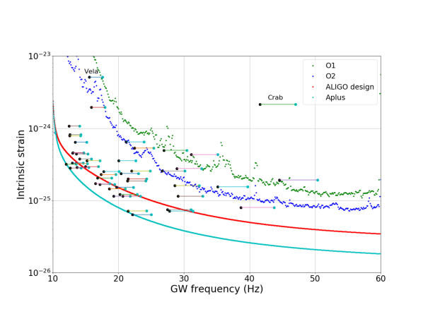
Figure 1: Spin-down limits for interesting pulsars (horizontal lines) and sensitivity estimates (other curves), both in terms of intrinsic strain vs. GW frequency. Spin-down limits are taken from Eq. (2) in the text. Sensitivity estimates are taken from Eq. (24) and the paragraph containing it.

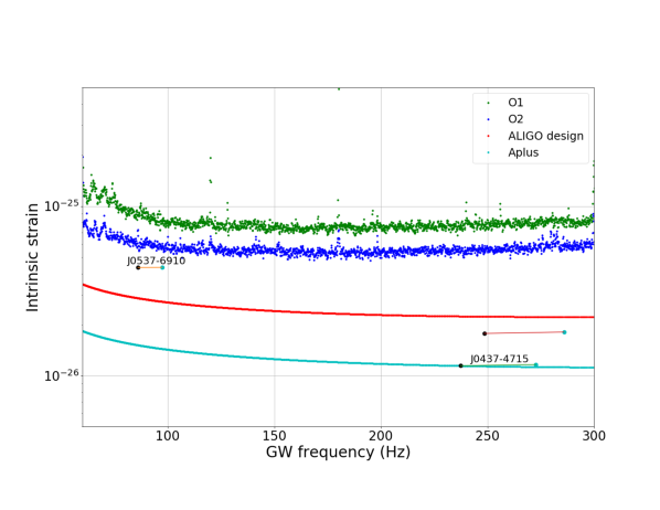
Figure 2: Same as the previous figure, for higher frequencies. There are fewer pulsars here, but the spin-down limits on $r$-mode amplitude are generally closer to predictions of saturation amplitude.

We express the sensitivity of each search in terms of upper limits on $h_{0}$ that can be placed in the absence of a detection. This is slightly pessimistic—the upper limits are conservative by design and it is plausible that a somewhat fainter signal could be detected—but it facilitates comparison with published upper limits from previous searches for continuous GWs. The precise definition of $h_{0}^{\mathrm{UL}}$ we use is the same as for instance in Ref. Abbott et al. (2018a). It is a 95% confidence limit on a population of injected signals with fixed $h_{0}$ but varying frequency (within a small band), frequency derivatives, and angles of inclination and polarization.

The sensitivity of a search of data from a single detector with stationary noise can be expressed as Wette (2012)

$$h_{0}^{\mathrm{UL}}=\frac{5}{2}\hat{\rho}\sqrt{\frac{S_{h}}{T_{d}}},$$ (24)

where $S_{h}$ is the strain noise power spectral density (PSD) and $T_{d}$ is the amount of data. (In general $T_{d}$ is less than the integration span $T$ times the number of interferometers due to maintenance, earthquakes, and so on.) For multiple detectors or non-stationary noise the PSD in Eq. (24) is replaced by a weighted sum Jaranowski et al. (1998); Cutler and Schutz (2005). For observations of many days at most sky locations, the sum is very close to the harmonic mean of noise PSDs, so we will use the harmonic mean when we give numbers later. The statistical factor $\hat{\rho}$ is iteratively estimated to sufficient precision using the method of Wette Wette (2012), using the template densities above and assuming that the upper limits are placed on 0.1 Hz frequency bands. (This upper limit band might be chosen differently for different searches, but its effect on sensitivity is negligible.) The factor $5\hat{\rho}/2$ ranges about 33–38 for the searches considered here, comparable to the factor for directed searches Abbott et al. (2018a) and about triple the factor for exact timing searches of known pulsars Aut (2019). We consider noise PSDs for O1 Sigg (2016a, b), O2 Kissel (2018a, b), Advanced LIGO design Barsotti et al. (2018a), and the recently funded A+ design Barsotti et al. (2018b). Hence we show four sensitivities: O1, O2, and one year integrations at Advanced LIGO and A+ design.

In Figs. 1 and 2 we plot our sensitivity measure vs. frequency for the four cases mentioned above, superposed on a set of spin-down limits for known pulsars from the ATNF catalogue Manchester et al. (2005). Most of the pulsars plotted have already been searched for GWs at $f=2\nu$ (and some also at $f=\nu$) in previous LIGO and Virgo papers based on exact pulsar timing solutions Aut (2019). Most of the pulsars whose spin-down limits are accessible with existing data are young and energetic (and sometimes glitchy) like the Crab, and most are shown in Fig. 1. As with known-timing searches, the Crab is the first spin-down limit to become accessible (already in O1), and several more including Vela soon follow. For later noise curves some middle-aged pulsars (in Fig. 1) and some recycled millisecond (in Fig. 2) pulsars become accessible. Most notable in Fig. 2 are J0537−6910 and J0437−4715. Due to its frequency and proximity to Earth, the latter has $\alpha_{\mathrm{sd}}$ of order $10^{-5}$—much lower, and hence more feasible, than the other accessible pulsars, although $h_{0}^{\mathrm{sd}}$ indicates this pulsar will require at least A+ to detect.

Not all of these pulsars are timed concurrently with LIGO-Virgo observing runs. Since the searches proposed here cover broad frequency bands, the uncertainty in frequency and spin-down parameters is not an issue—unlike the $\nu$ and $2\nu$ searches. Our proposed searches do suffer in sensitivity if a pulsar glitches during the integration, though; and they cannot account for the fluctuating torques likely in accreting systems. The glitch issue means that frequent x-ray timing of J0537−6910 will be important for future GW observing runs Andersson et al. (2018).

VI Discussion

We have shown that searches for continuous GWs from $r$-modes of known pulsars can beat the spin-down limits on some pulsars in existing data for reasonable computational costs. Although the $r$-mode amplitudes required for detection in such data are higher than predicted by theory, this work serves as a starting point for future improvements. Spin-down limits for many more pulsars will be attainable in the next few years.

Part of our goal is to point out what theory work could be most important to help observations. It is crucial to get the range of mode frequencies and spin-down parameters right, and helpful to narrow the range down and reduce costs. Relating frequencies and spin-down parameters more precisely to neutron star properties will also help measure the latter once a signal is detected.

The most important feature of the search is the $r$-mode frequency range. Avoided crossings such as that with $t$-modes in the crust could widen the parameter ranges of some pulsars well beyond what we consider here. Some pulsars could be undetectable without addressing the avoided crossings problem. Updated ranges of the $A$ and $B$ parameters of Eq. (4) would also help in terms of narrowing the parameter space and hence reducing the computational costs, which will grow to be substantial in coming years.

More estimates of saturation amplitudes would be helpful. This is a very difficult problem, and essentially has been addressed only by one approach Arras et al. (2003).

It would also help to be sure of the coherence time. If saturated $r$-modes in equilibrium with other modes occasionally experience phase jumps, this would render long coherent integrations of GW data problematic.

The coherence time issue leads into future work for data analysis: Accretion and glitches can also introduce issues which encourage development of alternatives to the straightforward coherent integrations considered here. Adaptations of semi-coherent techniques developed for other searches Sun et al. (2018); Suvorova et al. (2017); Dergachev (2012); Ashton et al. (2018) could be fruitful for $r$-modes from known pulsars too. For those pulsars with a known inclination angle, upgrading from the $\mathcal{F}$-statistic to the $\mathcal{G}$-statistic will also improve sensitivity.