The effect of telescope aperture, scattered light, and human vision on early measurements of sunspot and group numbers

Abstract

Early telescopic observations of sunspots were conducted with instruments of relatively small aperture. These instruments also suffered from a higher level of scattered light, and the human eye served as a “detector”. The eye’s ability to resolve small details depends on image contrast, and on average the intensity variations smaller than $\approx$ 3% contrast relative to background are not detected even if they are resolved by the telescope. Here we study the effect of these three parameters (telescope aperture, scattered light, and detection threshold of human vision) on sunspot number, group number, and area of sunspots. As an “ideal” dataset, we employ white-light (pseudo-continuum) observations from Helioseismic and Magnetic Imager (HMI) onboard of Solar Dynamics Observatory, and we model the appearance of sunspots by degrading the HMI images to corresponding telescope apertures with an added scattered light. We discuss the effects of different parameters on sunspot counts and derive functional dependencies, which could be used to normalize historical observations of sunspot counts to common denominator.

1 Introduction

Sunspot number is the longest time series representing the direct measurements of solar activity. The earliest telescope observations of sunspots go back to early 1610, when several scientists including Galileo Galilei, Thomas Harriot, Christoph Scheiner, and Johannes Fabricius (Hockey et al., 2014) observed dark areas of irregular shape now known as sunspots. (The first publication about sunspot observations was by Johannes Fabricius in 1611, in his “Narratio de maculis in sole observatis et apparente earum cum sole conversione”). After their discovery, the sunspots were observed by several scientists although some of them were searching for hypothesized planets orbiting the Sun and thus, their records could be biased towards dark features of a regular (round) shape (Zolotova & Ponyavin (2015), however, see Usoskin et al. (2015); Carrasco et al. (2018a) for opposing views). The later analysis of the historical records revealed that between 1645 and 1715 the sunspot sightings were extremely rare, and in fact, that period of prolong sunspot minimum was christened the Maunder (Grand) Minimum (Eddy, 1976). Despite lack of sunspots, the cosmogenic isotope records suggest that the magnetic cycles on the Sun did continue during the Maunder minimum (e.g., Beer et al., 1998; Cliver et al., 1998; Poluianov et al., 2014), and one of the speculations put forward was that, perhaps, during that time period the activity was represented by small sunspots, which were hard to observe with the existing telescopes. In fact, Vaquero et al. (2015) found that the solar cycle activity did continue during Maunder minimum, but with a low amplitudes of less than 5–10 Sunspot Number (SSN).

The return of sunspot activity was immediately noted by observers around the globe (see, for example, a letter to the Russian Czar Peter the Great by James Bruce, a Russian statesman and scientist known in Russia as Yakov Brus (Hockey et al., 2014). In this letter, dated 18 July 1716, Bruce writes that he observed a great number of spots on the Sun and adds that to his knowledge, sunspots were not seeing for a long time). In addition to a very low number of sunspots during the Maunder Minimum, most of them were located in one (southern) hemisphere (e.g., Ribes & Nesme-Ribes, 1993). The hemispheric asymmetry in sunspot formation and their very small number during the Maunder Minimum have been interpreted as a change in the character of solar activity. The reader can find a review of solar activity during Maunder minimum in Usoskin et al. (2015).

In addition, there could be the effects of instrumentation (telescopes) used for sunspot observations. In the past, the effect of telescope aperture on sunspot observations was largely discarded on somewhat general statements that the telescope apertures were sufficiently large to resolve even smallest pores (e.g., Hoyt & Schatten, 1996). However, this argument ignores the fact that many historical observers were stopping down the aperture of their telescopes using aperture masks. This was usually done to reduce the brightness of solar image and mitigate the heat load in prime focus. Thus, even if the telescopes used for astronomical observations had sufficiently large apertures during that historical period, solar observations were made with significantly smaller effective apertures. Furthermore, early observations of sunspots were eye observations, and additional glass filters (gray or green) were used to further reduce the intensity of the sunlight. In combination with imperfections of optical instruments of that time (e.g., spherical and chromatic aberrations) this will increase the level of the scattered light in the telescope, thus, potentially affecting the detectability of small sunspots. The effect of spherical and chromatic aberrations in sunspot observations in 18th century was considered by Svalgaard (2016, 2017), who set up an observing network of four amateur astronomers using original telescopes from the 18th Century with the same defects as the instruments available to observers of that period. Initial results found about one third of sunspot groups as compared with modern instruments.

Visual observations are also the subject of a physiological limitations of human eye – a property that is rarely considered in the framework of astronomical observations (but see pioneering work by Schaefer, 1991, 1993). In this paper, we investigate these effects on sunspot and group numbers, and sunspot areas. In Section 2 we describe our approach to modeling the effect of telescope aperture, scattered light, and human vision on sunspot and group number. Section 3 presents the results of modeling, and in Section 4, we discuss our findings.

2 Method and data

The detectability of sunspots depends on a resolving power of a telescope, observing conditions (atmospheric seeing), and the sensitivity of a detector (a human eye in historical observations). These are the three primary effects that we include in our investigation.

Angular resolution $\theta$ of an ideal telescope of diameter (aperture) $\rm D$ in a monochromatic light of wavelength $\lambda$ is determined by the Rayleigh criterion

$$\theta=1.22{\frac{\lambda}{D}}$$ (1)

Taking as an example, $\rm D$=0.1 m (or about 4 inches) and $\lambda$=555 nm (maximum daylight sensitivity of a normal sighted human eye), we arrive to $\theta\approx$ 1.40 seconds of arc. Assuming that solar pores vary in diameter between 1 and 5 arcseconds (Bruzek & Durrant, 1977), one would require a telescope with an aperture of 0.14 m (for 1 arcsec resolution) and 0.028 m (for 5 arcseonds resolution) to fully resolve pores of this size. Thus, the full aperture of telescopes used for astronomical observations during 1620–1675 (see Table 1 in Racine, 2004) should be sufficient to resolve large pores, while (large aperture) telescopes used after 1686 were capable to resolve even smallest pores.

After the invention of the telescope, their development for astronomical purposes was driven by a few individuals. Figure 1 in Racine (2004) shows a break in improvements of telescopes closer to the end of Maunder minimum period. The article also refers to King’s comment that “the success of the long telescopes of the seventeenth century was due, very largely, to the painstaking and persistent efforts of men like Hevelius, Huygens and J. D. Cassini. Indeed, after Cassini’s death in 1712, his successors were unable to see what he had already discovered, let alone add to the list, and the telescopes gradually fell into disuse” (King, 1979; Racine, 2004, page 133). Description of observations from that period of time often omits the details about the telescope aperture. Ribes & Nesme-Ribes (1993, see, Section 3.3) provide an indirect reference for instruments of that time that “usually a six-foot telescope would have an aperture of two inches and seven lines”, or, according to our calculations, about 0.065 m. As an additional complication, for solar observations the telescope apertures were often stopped down (the aperture was reduced by using a circular diaphragm in front of a telescope). This was done to reduce the amount of light in focal plane to prevent damage to focal lens or to the observer’s eye. Restricting the aperture by the means of diaphragm changes the resolution of the telescope, but unfortunately, while the fact of stopping down the diameter of telescope is mentioned in some historical records, the effective aperture is not provided. Based on authors’ personal experience with amateur astronomer observations of the Sun, prior to development of full aperture filters it was not uncommon to use the entrance diaphragm of 40–50 mm (about 1.57 – 1.97 inch) in diameter.

Atmospheric seeing conditions, optical quality of telescopes, and use of glass filters to further decrease the intensity of light in the focal plane had negative effects on sunspot observations too. Prior to 1733, objectives for all refractors employed a single lens design and were a subject of strong chromatic aberration. The chromatic aberration would result in a slight blurring of an image in a focal plane (due to a lateral shift of images in different wavelengths). In addition, optical aberrations and use of “neutral density” filters increased the amount of scattered light, and thus, reduced the contrast of images. This could have a major effect on detectability of small sunspots due to some physiological limitations of a human eye.

The ability of a human eye to detected the brightness variations is the subject of both spatial resolution and the image contrast (e.g., O’Carroll & Wiederman, 2014, and references therein). On average, for a human eye it is hard to detect the contrast variations less than about 3%. Figure 1 in O’Carroll & Wiederman (2014) provides an example of an intensity pattern used for testing human vision. It displays a periodic pattern of intensity variation with different spatial frequencies (in the horizontal direction) and with different image contrast (in the vertical direction). The frequency patterns are well-resolved at high contrast, but as contrast decreases, the patterns at high and low spatial frequencies gradually disappear.

The scattered light in the telescope (due to optical distortions, misalignment and filters) decreases the image contrast, and thus, it would reduce the detectability of pores and small sunspots. So far, this effect was not taken into consideration in computation of sunspot number.

To model the effect of telescope aperture and image contrast on sunspot time series, we use the modern white-light (a pseudo-continuum) images from the Helioseismic and Magnetic Imager (HMI, Scherrer et al., 2012) on board Solar Dynamics Observatory (SDO). We treat the HMI white-light image as the reference representing true distribution of sunspots on solar surface. To mimic the appearance of observations with the telescope of a different aperture, we convolve the HMI images with a point-spread function of an appropriate width. For simplicity, we use a symmetric 2D Gaussian function for that matter. The Rayleigh criterion represents the angular separation between two point sources equal to the radius of the Airy disk. FWHM of Airy disk $FWHM_{Airy}=1.024\lambda D$, where $\lambda$ is the wavelength and $D$ is the telescope aperture. Gaussian function provides a good approximation of intensity distribution in Airy disk, and thus, in this work we employ a normalized FWHM of Gaussian function to represent the telescope aperture. $FWHM_{Gauss}=2\sigma\sqrt{2\ln 2}$, where $\sigma$ is the standard deviation. For each image convolved with the Gaussian function, we apply intensity threshold to identify sunspots and pores, and we group the identified features based on their separation in latitude and longitude. According to our definition, to be considered as a group, sunspots should be located within 15 degrees in longitude and 7 degrees in latitude from the leading feature (spot or pore). These criteria are based on Tlatova et al. (2018). The grouping is done by starting from the largest spot on each image, and identifying all spots that satisfy distance criteria to be counted as a group. The spots that are identified on this step as a group are excluded, and the process is repeated until all spots on the solar disk are identified with their respective groups.

For each HMI image, we compute the sunspot number as

$$SSN=k~{}(10~{}GN+N_{S}),$$ (2)

where $GN$ is number of groups (or group number), and $N_{S}$ is the number of spots for this image. Classical formula for SSN includes additional scaling $k$-coefficient, which is used as a normalization between different observers. Here we assume $k$ = 1. The group and sunspot number identification is repeated for the same “ideal telescope” image degraded to represent observations with different telescope apertures. We note that in this analysis we did not try to develop an algorithm for a perfect identification of sunspots and groups. The goal is to have a reasonable approach and apply such approach consistently to images representing telescopes of different aperture to see the overall tendency for changes in sunspot and group number due to telescope aperture. To mimic the effect of a scattered light, we convolved the images with a scattering function representing 2% or 5% (two different levels of scattered light) of mean intensity of solar image. The resulting images were used to identify sunspots. This level of a scattered light is consistent (if not low) with the modern telescope observations of a Mercury transit (e.g., Briand et al., 2006).

To model the effect of human vision, when identifying the sunspots, we applied a 3% contrast criterion. Intensity variations less than 3% were not counted as sunspots.

3 Computation of sunspot and group numbers

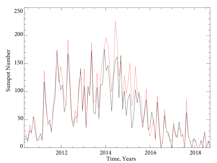
Figure 2: Monthly international sunspot number from SILSO (black) and computed by our algorithm (red).

Figure 1 shows example of an HMI image with groups identified by our algorithm. Sunspot number (SSN) computed by our algorithm for this image is 46 (3 groups and 16 sunspots). For comparison, the sunspot number from Sunspot Index and Long-term Solar Observations (SILSO) World Data Center lists SSN=45 for the same day. Figure 2 shows international sunspot number time series and computed by us using full disk images from HMI/SDO. In this comparison, only one daily measurement per month was used. Two time series are in good agreement (Pearson correlation coefficient, r_P=0.963), both showing the solar cycle variation for sunspot cycle 24. Other time series that we compared our SSN determination with is Sunspot Tracking and Recognition Algorithm (STARA Watson et al., 2009). The latter used white-light observations from the Michelson Doppler Imager (MDI) on board Solar and Heliospheric Observatory (SOHO). Daily (one image per month) sunspot number determined by our algorithm also strongly correlate with STARA SSN (r_P=0.957) although our SSN tend to show a slightly lower values in (local) minima of time series. We explain this by lower spatial resolution of the original datasets used by STARA. This could be related to a difference in a pixel size of images from two datasets. We use HMI data with pixel size of about 0.5 arcseconds, while STARA employed MDI/SOHO data with pixel size of about 2 arcseconds. Based on this comparison with two independent (SILSO and STARA) datasets, we conclude that our algorithm performs sufficiently well for identifying the individual sunspots and sunspot groups on HMI white light images.

As the next step, we repeated our identification of sunspots for degraded HMI images mimicking observations with lower spatial resolution and with added scattered light. As expected, the sunspot number decreases with decreasing telescope aperture. For example, using observations shown in Figure 1a degraded to 2 inch telescope (without scattered light) returns SSN = 39 (3 groups and 9 sunspots). Table 1 shows SSN and GN for other apertures corresponding to this image including naked eye (0.13 inch or about 3 mm).

Figures 3 - 5 show Sunspot Number (SSN), Group Number (GN) and area of sunspots as function of the telescope aperture. The data are normalized to the maximum of each parameter as observed by the telescope with 130 mm (5.12 inch) aperture and in the absence of scattered light. The plots include all sunspots and groups identified by our method in solar cycle 24. The data points shown in Figures 3–5 are also provided in Table 2. Coefficients of fitted curves are listed in Table 3. In comparison with 130 mm aperture, an observer equipped with a 40 mm aperture telescope will measure about 60% SSN, 78% GN, and 90% sunspot areas. Having 5% of scattered light will further reduce these values to 55%, 75%, and 86%, accordingly. The decrease in telescope aperture beyond 40 mm results in a rapid decrease in SSN, GN, and sunspot area. Out of three parameters, SSN number shows stronger dependence on the level of scattered light (Figure 3), and sunspot areas are much less affected (Figure 5). This agrees with Nagovitsyn & Georgieva (2017) findings that sunspot area is a more robust measure of sunspot activity as compared with SSN and GN. The scattered light has a stronger effect on telescopes with larger apertures. Thus, for example, adding 5% scattered light to 130 mm aperture telescope leads to about 20% reduction in SSN (Figure 3) and 10% reduction in GN (Figure 4). The effect, however, is much smaller for small apertures. We see this as indication that for small apertures, the diffraction (telescope resolution) has much stronger effect as compared with the scattered light, and for larger apertures, the latter becomes more important. In the handbook for amateur solar observations, Beck et al. (1995) recommend on optimal telescope aperture of 80 mm. This recommendation is based on a typical diameter of near-ground turbulent convection cells, and the resolving power necessary to see the smallest spots. Telescopes with larger aperture will have an image blurred (and hence, less contrasted) due to the light passing through multiple convection cells as compared with 80 mm aperture scope, which images will be affected by a single cell. The results shown in Figures 3–5 indicate that a telescope with such aperture performs sufficiently well even in presence of the scattered light although our current calculations do not take into account the effects of the atmospheric seeing.

4 Discussion

Our results clearly demonstrate how the telescope aperture, its optical quality (scattered light) in combination with physiological limitations of human vision can affect the detectability of sunspots. We think that previous, somewhat generic, claims that during the Maunder minimum the telescopes had sufficiently high apertures to resolve ”regular diameter” sunspots may ignore the fact that for solar observations the entrance aperture of telescopes was usually stopped down using a diaphragm of a much smaller diameter. The latter would result in reducing the resolving power of an instrument. While the historical records do mention stopping down the telescope aperture, no aperture of the diaphragm is usually provided. Moreover, the early telescopes were not perfect in respect to their optical properties and thus, may have had a significant level of scattered light.

There are some historical records that seem to support the notion that the detectability of sunspots could be severely affected by the observational conditions (e.g., the instrument quality, the atmospheric seeing conditions and the observer’s vision). For example, Table 1 and Figure 1 in Vaquero et al. (2007) provides sunspot records for the observations taken simultaneously by different observers. For June 3, 1769 observations, number of groups (GN) detected by different observers vary between 1 and 10. Even for observers in the same geographic location (e.g., Paris), the sunspot group number vary significantly: GN=1 (Darquier), GN=5 (Bailly), and GN=9 (Messier). Based on Tisserand (1881), Darquier probably used a small aperture instrument (a quadrant with 27 inch focal length telescope). According to de La Lande & Messier (1769) letters, Messier used achromatic telescope (refractor) with 12 feet focus, 3.75 inch aperture and 180 magnification, while Bailly was using a reflector of 30 inch focus and 4.5 inch aperture. Messier also mentions that seeing conditions were not great (“vapors” and clouds). This seems to agree with our conjecture that observing with small aperture telescope (Darquier) returns small number of groups, and using a telescope with less scattered light (Messier) allows detecting a larger number of groups as compared with a telescope of similar aperture but higher level of scattered light (Bailly).

The detectability of sunspots could also be affected by difference in persons’ vision, which is hard, if possible to characterise without additional information. As one example, we use an interesting handwritten note on the sunspot drawing taken at Mount Wilson Observatory (MWO) on 15 February 1999 (scanned image available via UCLA server at ftp://howard.astro.ucla.edu/pub/obs/drawings does not contain this note). This day, two naked eye sunspots were present on the Sun. However, the note on the drawing indicates that out of three observers, L.W. (Larry Webster) saw 2 naked eye sunspots, P.G. (Peter Gilman) saw only one (lower) sunspot, and S.P. (Steve Padilla) saw none of naked eye sunspots. These were the trained professional observers, who probably knew about the presence of naked-eye sunspots on solar disk the day of observations, but still each would see them differently. While the naked eye sunspots are not the subject of our paper, we use this as an example of how human vision could affect the detectability of sunspots.

The atmospheric seeing is other unknown parameter that could affected the detectalibity of sunspots. For historical observations, it is hard if possible to estimate, but for a pictorial example, we refer the reader to sunspot drawings made at MWO over three consecutive days 15-17 December 1969. In the first drawing (15 Dec. 1969), taken under almost excellent atmospheric seeing conditions (seeing = 4+ on a scale 1–5), the observer identified 9 different groups with large number of small sunspots and pores. Second image was taken on 16 Dec. 1969 under extremely poor conditions (seeing = 1) and only 4 groups consisting large spots and a few pores were identified. Observations taken on 17 Dec. 1969 under good seeing  = 3 conditions again show 10 groups with a large number of small pores.

Figure 6 shows sunspot number (SSN) computed for cycle 24 as if sunspots were observed with the small aperture telescopes and 5% scattered light. For a reference, Galileo used 0.5 inch telescope for his early sunspot observations. (The largest telescope that Galileo used had an aperture of 5.1 cm, but was usually stopped down to 2.6 cm, or about one inch. However, the tests of one of Galileo’s first telescopes showed the resolving power corresponding to about 0.5 inch aperture (resolving $\approx$ 10 arcsec and larger features, Arlt et al. (2016).) Schwabe employed 1.25 inch instrument, and Wolf used 2.5 inch telescope. It is clear that naked eye observations would not allow detecting the solar cycle variations for cycle similar in amplitude to cycle 24. Galileo and Schwabe instruments would be marginal in detecting a cycle similar in amplitude to cycle 24 if one takes into account the scattered light and 3% detectability threshold of human eye. Observations with telescopes larger than 2 inch in aperture will detect the cycle variations albeit with a significantly smaller amplitude (about 50% less according to Figure 6, compare black and blue lines).

While some effects of human vision on sunspot number the cannot be fully quantified (e.g., change in contrast detection sensitivity with age), our results offer a path for normalizing historical SSN time series to bring observations taken with the telescopes of different apertures and scattered light in line with each other. One interesting observation that the reader can note from Figure 3 and Table 2 is that for 60 mm ($\approx$ 2.5 inch) telescope, SSN is about 60% of “true” SSN. Although it could be a coincidence, this is close to $k$-coefficient used by Wolf when computing sunspot number (see Equation 2).

Our results indicate that sunspot number (SSN) is affected by the telescope quality (including scattered light), human vision, and the observing conditions more than group number and sunspot areas. In their turn, sunspot area is a much more robust measure than SSN and GN. However, while sunspot areas could be derived even from the very early drawings, they might be a subject of large uncertainties due to different drawing styles, lack of proper scaling, and some may even be unsuitable for a scientific use (e.g., Arlt et al., 2016; Senthamizh Pavai et al., 2015; Carrasco et al., 2018b; Fujiyama et al., 2019).

Many details of early telescopic observations are unknown including focal length, aperture, and other characteristics on the telescopes, the used methodology, and even the aims of these observations (Muñoz-Jaramillo & Vaquero, 2019). While we base some of our interpretation on the assumption that all early observations were taken with small aperture telescopes, it is likely, that the telescopes of different (small, medium and large) apertures were used. A similar mix of instruments was also used for recording sunspot numbers in later periods (18th and 19th centuries). Thus, the results of our study could also be applicable to sunspot visual observations taken in other periods during last four centuries, not only to the earliest observations.

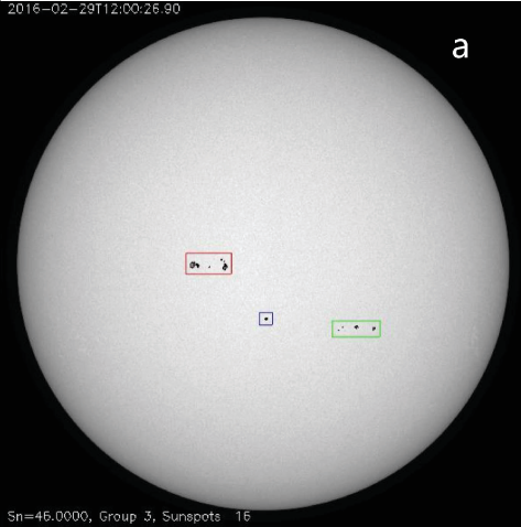
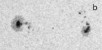
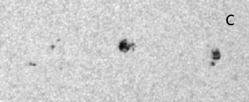
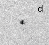
Figure 1: Example of full disk HMI image observed on 29 Feb. 2016 at 00:26 UT (a). Three colored boxes mark location of groups selected by our algorithm. Adjacent panels show magnifying view of each group. For group in panel (b), the algorithm identified 9 sunspots, panel (c) – 6 sunspots, and panel (d) one spot.

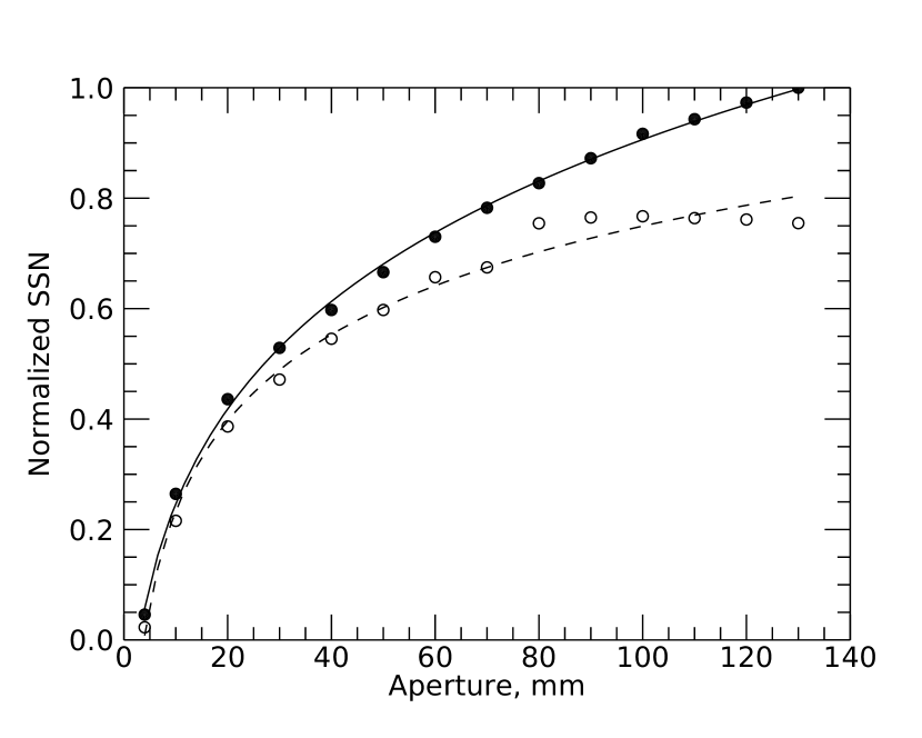
Figure 3: Sunspot number (SSN) computed from HMI images as a function of effective aperture of a telescope without scattered light (filled circles) and with 5% scattered light (open circles). Data are normalized to maximum value of SSN without scattered light. Solid lines show least-square fitting by logsquare function (see coefficients in Table 3).

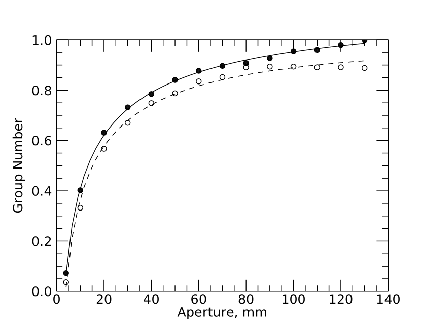
Figure 4: Same as Figure 3, but for group number (GN).

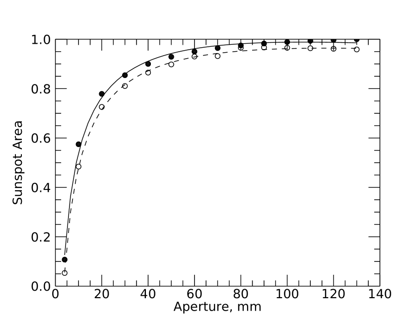
Figure 5: Same as Figure 3, but for sunspot area.

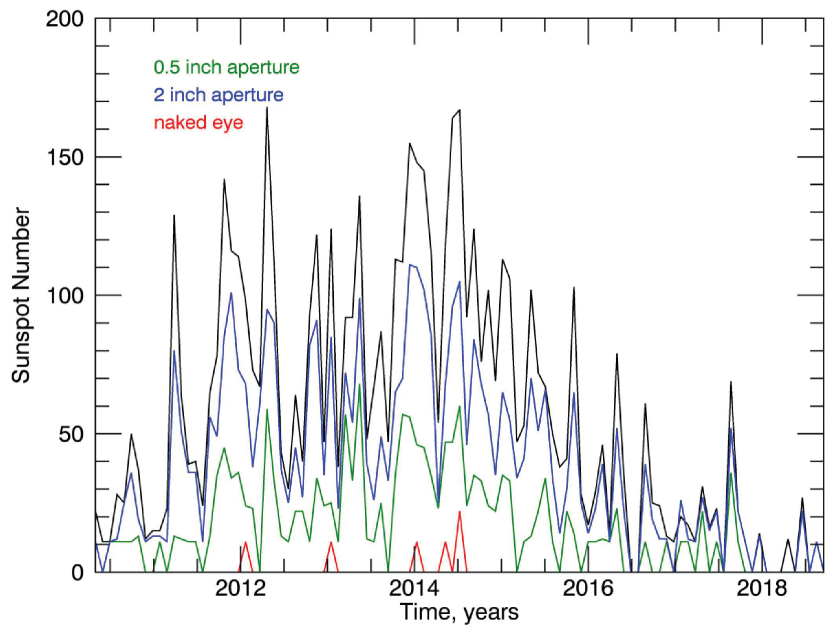
Figure 6: Monthly sunspot number (SSN) in cycle 24 computed for telescopes of different aperture: full resolution (black), 2 inch aperture (blue), 0.5 inch (green) and naked eye observations (red).

Table 1: Change in SSN as function of telescope aperture for image shown in Figure 1

Aperture	GN	Spots	SSN
(inch)
ideal	3	16	46
2.00	3	9	39
1.00	3	6	36
0.64	3	4	34
0.57	2	3	23
0.37	1	2	12
0.13	0	0	0

Table 2: Sunspot, Group number and sunspot area without scattered light and with 5% scattered light

mm	SSN	SSN+S	Area	Area+S	GN	GN+S
4	0.046	0.023	0.108	0.053	0.073	0.036
10	0.265	0.216	0.575	0.484	0.402	0.332
20	0.436	0.387	0.779	0.726	0.631	0.567
30	0.529	0.472	0.854	0.811	0.732	0.670
40	0.598	0.545	0.900	0.865	0.785	0.749
50	0.666	0.598	0.929	0.898	0.841	0.788
60	0.730	0.657	0.950	0.930	0.877	0.835
70	0.783	0.675	0.964	0.932	0.897	0.852
80	0.827	0.755	0.975	0.965	0.908	0.891
90	0.872	0.765	0.983	0.967	0.927	0.894
100	0.917	0.767	0.989	0.965	0.955	0.894
110	0.943	0.764	0.994	0.964	0.961	0.891
120	0.973	0.761	0.997	0.961	0.980	0.891
130	1.000	0.755	1.000	0.959	1.000	0.888

Table 3: Coefficients of $y=a_{0}+a_{1}\log(x)+a_{2}\log^{2}(x)$ function fitted to data shown in Figures 3–5

	SSN	SSN+S	GN	GN+S	Area	Area+S
a0	-0.153	-0.356	-0.576	-0.666	-0.754	-0.843
a1	0.271	0.626	1.210	1.286	1.717	1.747
a2	0.129	-0.037	-0.222	-0.254	-0.423	-0.422

References

- Arlt et al. (2016) Arlt R., Senthamizh Pavai V., Schmiel C., Spada F., 2016, A&A, 595, A104
- Beck et al. (1995) Beck R., Hilbrecht H., Reinsch K., Voelker P., 1995, Solar astronomy handbook. Willmann-Bell
- Beer et al. (1998) Beer J., Tobias S., Weiss N., 1998, Sol. Phys., 181, 237
- Briand et al. (2006) Briand C., Mattig W., Ceppatelli G., Mainella G., 2006, Sol. Phys., 234, 187
- Bruzek & Durrant (1977) Bruzek A., Durrant C. J., eds, 1977, Illustrated glossary for solar and solar-terrestrial physics Astrophysics and Space Science Library Vol. 69, doi:10.1007/978-94-010-1245-4.
- Carrasco et al. (2018a) Carrasco V. M. S., Vaquero J. M., Gallego M. C., 2018a, Sol. Phys., 293, 51
- Carrasco et al. (2018b) Carrasco V. M. S., Vaquero J. M., Arlt R., Gallego M. C., 2018b, Sol. Phys., 293, 102
- Cliver et al. (1998) Cliver E. W., Boriakoff V., Bounar K. H., 1998, Geophys. Res. Lett., 25, 897
- Eddy (1976) Eddy J. A., 1976, Science, 192, 1189
- Fujiyama et al. (2019) Fujiyama M., et al., 2019, Sol. Phys., 294, 43
- Hockey et al. (2014) Hockey T., Trimble V., Williams T. R., Bracher K., Jarrell R. A., Marchéll J. D., Palmeri J., Green D. W. E., eds, 2014, Biographical Encyclopedia of Astronomers, 2 edn. Springer, New York, NY, doi:10.1007/978-1-4419-9917-7
- Hoyt & Schatten (1996) Hoyt D. V., Schatten K. H., 1996, Sol. Phys., 165, 181
- King (1979) King H. C., 1979, The History of the Telescope. Dover Publications, New York
- Muñoz-Jaramillo & Vaquero (2019) Muñoz-Jaramillo A., Vaquero J. M., 2019, Nature Astronomy, 3, 205
- Nagovitsyn & Georgieva (2017) Nagovitsyn Y. A., Georgieva K., 2017, Geomagnetism and Aeronomy, 57, 783
- O’Carroll & Wiederman (2014) O’Carroll D. C., Wiederman S. D., 2014, Phil. Trans. R. Soc. B, 369, 20130043
- Poluianov et al. (2014) Poluianov S. V., Usoskin I. G., Kovaltsov G. A., 2014, Sol. Phys., 289, 4701
- Racine (2004) Racine R., 2004, PASP, 116, 77
- Ribes & Nesme-Ribes (1993) Ribes J. C., Nesme-Ribes E., 1993, A&A, 276, 549
- Schaefer (1991) Schaefer B. E., 1991, QJRAS, 32, 35
- Schaefer (1993) Schaefer B. E., 1993, ApJ, 411, 909
- Scherrer et al. (2012) Scherrer P. H., et al., 2012, Sol. Phys., 275, 207
- Senthamizh Pavai et al. (2015) Senthamizh Pavai V., Arlt R., Dasi-Espuig M., Krivova N. A., Solanki S. K., 2015, A&A, 584, A73
- Svalgaard (2016) Svalgaard L., 2016, in AAS/Solar Physics Division Abstracts #47. AAS/Solar Physics Division Meeting. p. 10.12
- Svalgaard (2017) Svalgaard L., 2017, Sol. Phys., 292, 4
- Tisserand (1881) Tisserand F., 1881, Astronomical register, 19, 218
- Tlatova et al. (2018) Tlatova K., et al., 2018, Sol. Phys., 293, 118
- Usoskin et al. (2015) Usoskin I. G., et al., 2015, A&A, 581, A95
- Vaquero et al. (2007) Vaquero J. M., Trigo R. M., Gallego M. C., Moreno-Corral M. A., 2007, Sol. Phys., 240, 165
- Vaquero et al. (2015) Vaquero J. M., Kovaltsov G. A., Usoskin I. G., Carrasco V. M. S., Gallego M. C., 2015, A&A, 577, A71
- Watson et al. (2009) Watson F., Fletcher L., Dalla S., Marshall S., 2009, Sol. Phys., 260, 5
- Zolotova & Ponyavin (2015) Zolotova N. V., Ponyavin D. I., 2015, ApJ, 800, 42
- de La Lande & Messier (1769) de La Lande M., Messier M., 1769, Philosophical Transactions of the Royal Society of London Series I, 59, 374