Infrared $K_{s}$-band Photometry of Field RR Lyrae Variable Stars

Abstract

We present multi-epoch infrared photometry in the $K_{s}$-band for 74 bright RR Lyrae variable stars tied directly to the 2MASS photometric system. We systematize additional $K$-band photometry from the literature to the 2MASS system and combine it to obtain photometry for 146 RR Lyrae stars on a consistent, modern system. A set of outlier stars in the literature photometry is identified and discussed. Reddening estimates for each star were gathered from the literature and combined to provide an estimate of the interstellar absorption affecting each star, and we find excellent agreement with another source in the literature. We utilize trigonometric parallaxes from the Second Data Release of ESA’s Gaia astrometric satellite to determine the absolute magnitude, $M_{K_{s}}$ for each of these stars, and analyze them using the astrometry based luminosity prescription to obtain a parallax-based calibration of $M_{K}$(RR). Our period-luminosity-metallicity relationship is $M_{K_{s}}=(-2.8\pm 0.2)(\log P+0.27)+(0.12\pm 0.02)([\mathrm{Fe/H}]+1.3)-(0.41\pm 0.03)$ mag. A Gaia global zero-point error of $\pi_{zp}=-0.042\pm 0.013\,$mas is determined for this sample of RR Lyrae stars.

1 Introduction

For many decades, the RR Lyrae variable stars (RRL) have played a fundamental role in establishing the distance scale for old stellar populations, including globular clusters, the Galactic bulge, and the Magellanic clouds (e.g., see the review by Cacciari (2013)). The resulting calibrations of the visual absolute magnitude, $M_{V}$(RR) and its near-infrared analog, $M_{K}$(RR), provide a critical lower rung on the intergalactic distance ladder (Dambis et al., 2013; Gaia Collaboration et al., 2017). These stars have also proved useful in mapping Galactic stellar overdensities and streams, and interacting galaxies (e.g., Vivas & Zinn (2006); Belokurov et al. (2017)). Furthermore, accurate distance measurements to globular clusters and nearby galaxies are critical to determining the main-sequence turn-off ages to these systems, with a 1% uncertainty in distance leading to $\sim$2% uncertainty in the derived age of a given system (Chaboyer et al., 1996). Accurate ages for globular clusters can set a stringent limit on the age of the Universe, providing an important independent check on that age from recent precision cosmology studies (Planck Collaboration et al., 2018), and they can be used to look for trends in the chronology and metal-enrichment histories of the old stellar populations in our Galaxy, thereby constraining models of its formation and early evolution (Dékány et al., 2018).

Previous calibrations of the RRL absolute magnitude have taken a variety of approaches, including utilizing the Baade-Wesslink and infrared flux methods (e.g., Liu & Janes (1990), Jones et al. (1992), Skillen et al. (1993), and references therein), statistical parallax (e.g, Layden et al. (1996); Fernley et al. (1998); Dambis et al. (2013) and references therein), and fitting the main sequences of globular clusters to field subdwarfs with high-quality parallaxes (Carretta et al., 2000). Despite these efforts, a high degree of uncertainty remains. For example, the $M_{K}$(RR) calibrations listed in Table 2 of Cacciari (2013) range over 0.14 mag at a fiducial metallicity.

Direct trigonometric parallax is the preferred method of obtaining the distance to any stellar source, yet even using precision astrometry from the Hipparcos satellite and the Hubble Space Telescope, the few RRL closest to the Sun have not yet provided a definitive RRL luminosity calibration (e.g., see Table 1 of Gaia Collaboration et al. (2017) and references therein). It was with these ideas in mind that our team proposed to use NASA’s Space Interferometry Mission PlanetQuest (SIM-PQ) astrometric satellite (Unwin et al., 2008), which was designed to deliver parallaxes with precisions at the micro-arcsecond level, in order to determine the distance scale to Population II objects. Our key project was awarded 1330 hours of observing time on SIM-PQ to obtain parallaxes for 21 globular clusters, 60 field RRL, and 60 metal-poor field subdwarf stars (Chaboyer et al., 2005). A goal of the project was to calibrate the RRL absolute magnitude scales, $M_{V}$(RR) and $M_{K}$(RR), with unprecedented precision. At that time, we developed a list of potential target RRL, and began ground-based photometric time-series observations in the $VI_{C}K_{s}$ passbands to provide phased light curves and mean apparent magnitudes in support of the space-based astrometry. Unfortunately, delays in the SIM-PQ program led to cost overruns, and though a simplified version of the mission called SIM-Lite (Marr, Shao & Goullioud, 2010) briefly replaced it, the project was eventually discontinued at the end of 2010. This paper will focus on our $K_{s}$ observations and the resulting $M_{K_{s}}(RR)$ calibration, along with comparisons with infrared work by other researchers.

Though many studies have pushed forward with the goal of refining the RRL luminosity calibration in the intervening years, a revolutionary advancement through space-based precision astrometry has been absent until recently. Fortunately, this situation is changing rapidly as results from the European Space Agency’s Gaia satellite (Gaia Collaboration et al., 2016a) become available. Preliminary parallaxes from the Gaia Data Release 1 (Gaia Collaboration et al., 2016b) for several hundred field RRL were analyzed by Gaia Collaboration et al. (2017), who used single-epoch $K_{s}$-band apparent magnitudes and interstellar reddening values compiled by Dambis et al. (2013) to determine preliminary infrared period-luminosity (PL) and period-luminosity-metallicity (PLZ) relations. The second data release, DR2, (Gaia Collaboration et al., 2018a) contained significantly improved astrometry, and was used by Muraveva et al. (2018), again using photometric data from Dambis et al. (2013), to further improve the infrared PL and PLZ relations. Still further improvements in the Gaia parallaxes are expected in the third and final data releases, which are currently scheduled for 2020 and 2022, respectively.

As these improvements unfold, we felt it was timely to contribute our multi-epoch apparent $K_{s}$ photometry of field RRL and integrate them with the existing photometry for these stars to provide an optimal photometric database for present and future PL and PLZ analyses. In Section 2 of this paper, we describe the selection of our sample of RRL and compile pre-existing data including interstellar reddening estimates, pulsation periods, and metallicities. In Section 3 we describe our infrared imaging observations, while in Section 4 we present our methods for photometric measurement and calibration. Our method for fitting the phased light curves with templates of characteristic shape is presented in Section 5, and details concerning the photometric uncertainties are assessed in Section 6. In Section 7 we compare our photometry with that of other sources and integrate them into a comprehensive database useful for future studies. We utilize the DR2 parallaxes in Section 8 using advanced statistical methods to determine our version of the PLZ relation. We present our conclusions in Section 9, and in an Appendix we provide notes on the light curves of individual stars.

2 Sample Selection

Because SIM-PQ was designed as a targeted instrument rather than an all-sky survey satellite like Gaia, we developed a target list for our $K_{s}$-band photometry program based on the 144 RRL in Fernley et al. (1998) and supplemented it with stars from the RRL lists of Layden (1994) and other sources, resulting in a working database of 172 RRL. Careful prioritization based on astrophysical properties like metallicity, period, Oosterhoff group, and kinematics allowed us to focus attention on the most relevant stars. We also prioritized stars with no $K$-band photometry in the literature, and stars whose literaturephotometry appeared to be of lower quality. We tended to avoid stars that were known to exhibit the Blazhko effect. Due to a variety of factors including sky visibility and weather, we ultimately obtained $K_{s}$-band photometry for the first 75 stars listed in Table 1. The column labeled “ID (2MASS)” contains each star’s unique identifier in the Two-Micron All-Sky Survey (2MASS) of Skrutskie et al. (2006), which is the sexigesimal equatorial coordinates for the star coded in the standard catalog format. The next columns contain each star’s Galactic longitude and latitude ($l$, $b$) in degrees. For most stars, we obtained two estimates of the period, one from Fernley et al. (1998) and a second from a recent inspection of the International Variable Star Index (VSX). These two values are usually very similar, and are reported in Table 1 as $P_{F98}$ and $P_{VSX}$, respectively.

Table 1: The RR Lyrae Sample and Literature Data

Star	ID (2MASS)	$l$	$b$	$P_{F98}$	$P_{VSX}$	[Fe/H]L94	[Fe/H]F98	$N_{src}$	$E_{SF11}$	$E_{B92}$	$E_{F98}$	$K_{F98}$	Ref	Comment
DM And	23320072+3511488	105.11	–24.91	0.630389	0.6304244	–2.32	$\cdots$	0	0.081	$\cdots$	$\cdots$	$\cdots$	$\cdots$	$\cdots$
WY Ant	10160494–2943423	266.94	+22.08	0.574312	0.5743427	–1.66	–1.48	2	0.059	0.05	0.07	9.64	1	bw36
$\cdots$	$\cdots$	$\cdots$	$\cdots$	$\cdots$	$\cdots$	$\cdots$	$\cdots$	$\cdots$	$\cdots$	$\cdots$	$\cdots$	$\cdots$	$\cdots$	$\cdots$
AU Vir	13244801–0658455	317.45	+54.95	0.343230	0.3432307	$\cdots$	–1.50	3	0.025	$\cdots$	–0.01	10.81	3	RRc
AV Vir	13201156+0911163	325.01	+70.82	0.656908	0.6569073	–1.32	–1.25	2	0.027	$\cdots$	–0.01	10.63	2	$\cdots$
NSV 660	01545017+0015007	154.61	–58.67	$\cdots$	0.636589	$\cdots$	$\cdots$	0	0.031	$\cdots$	$\cdots$	$\cdots$	$\cdots$	Szabó et al. (2014)
SW And	00234308+2924036	115.72	–33.08	0.442279	0.442262	–0.38	–0.24	6	0.039	0.09	0.07	8.54	1	B? bw10, bw25
$\cdots$	$\cdots$	$\cdots$	$\cdots$	$\cdots$	$\cdots$	$\cdots$	$\cdots$	$\cdots$	$\cdots$	$\cdots$	$\cdots$	$\cdots$	$\cdots$	$\cdots$
AF Vir	14280981+0632438	355.47	+59.16	0.483722	0.483747	–1.46	–1.33	2	0.021	$\cdots$	0.05	10.75	3	$\cdots$
BN Vul	19275606+2420505	58.63	+3.41	0.594125	0.5941318	$\cdots$	–1.61	1	1.053	0.44	0.41	8.81	2	$\cdots$

Note. — (This table is available in its entirety in machine-readable form.)

2.1 Stellar Abundances from the Literature

There are two principal sources of metallicities available in the literature for the RRL in Table 1: the spectroscopic study of Layden (1994) (which was calibrated to the globular cluster metallicity scale of Zinn & West (1984)) and the compilation of [Fe/H] sources by Fernley et al. (1998), which includes values from Layden (1994). These sources provided most of the [Fe/H] values for the bright RRL in the catalog of Beers et al. (2000). Dambis et al. (2013) drew their metallicities from this catalog, and the Dambis values were used in turn by the recent RRL PLZ studies utilizing Gaia astrometry (Gaia Collaboration et al., 2017; Muraveva et al., 2018). These values are listed in Table 1 as [Fe/H]_L94 and [Fe/H]_F98 respectively, and the column labeled $N_{src}$ lists the number of metallicity estimates from independent sources in the Fernley et al. (1998) compilation.

Figure 1 shows the relationship between these metallicities for the 93 stars in our working database of 172 objects that have both metallicity measures, where the difference $\Delta$[Fe/H] is calculated in the sense Layden minus Fernley. It is apparent that stars utilizing data from a larger number of sources ($N_{src}$) have a smaller scatter in this figure, and the statistics in Table 2 support this claim. Specifically, as $N_{src}$ increases from two to five-or-more sources, the standard deviation $\sigma$ of the metallicity difference decreases from 0.20 to 0.08 dex. Because the ranking of [Fe/H] values compiled from multiple sources is demonstrably better than those of a single source, we adopt the Fernley et al. (1998) values as the primary source of our metallicities from Table 1, and when absent, we use the value from Layden (1994). In total, there were 21 stars for which the Layden (1994) was the only source.

The mean metallicity difference, shown in the second column of Table 2, is slightly negative for each line. Depending on the weighting scheme utilized to combine them, the typical value is about $-0.06$ dex in the sense that metallicities from Fernley et al. (1998) are systematically more metal-rich than those of Layden (1994). This difference is small, and in past works (Beers et al., 2000; Dambis et al., 2013) the values from these two sources have been utilized without any systematic corrections. We too are inclined to combine the values from the two sources without correction, but note that shifting the Layden values onto the Fernley system, or vice versa, are also reasonable approaches. Clearly, a well-documented combination of all the currently available literature values of [Fe/H] for all field RRL is warranted.

The standard deviations $\sigma$ in Table 2 contain information about the typical uncertainties in the [Fe/H] measures of both Layden (1994) and of Fernley et al. (1998). Table 9 of Layden (1994) reports two estimates of the [Fe/H] uncertainty for each star. For each group of $N_{star}$ stars from a line shown in Table 2, we calculated the mean of these observational uncertainties and present it as $\overline{\sigma_{L94}}$. We then subtracted that in quadrature from the value of $\sigma$ to obtain an estimate of the typical uncertainty in the [Fe/H] value from Fernley et al. (1998) for stars in that group, $\overline{\sigma_{F98}}$. Statistically, these values may be used to weight the impact of different stars in the overall PLZ relation. Notice that for two groups, the estimated uncertainty $\overline{\sigma_{L94}}$ accounts for all of the dispersion in the metallicity difference, so we set the entries for $\overline{\sigma_{F98}}$ to zero for these lines in Table 2, even though it is unlikely the Fernley metallicities have no observational uncertainty.

The data in Table 2 are broadly consistent with the behavior $\sigma_{[\mathrm{Fe/H}]}=0.22~{}N_{src}^{-0.5}$ dex for stars having metallicities in Fernley et al. (1998). For the stars with metallicities from Layden (1994) alone we suggest $\sigma_{[\mathrm{Fe/H}]}=0.15$ dex, based on the $\overline{\sigma_{L94}}$ values in Table 2 and statements made in Layden (1994). These values should be suitable for statistical weighting and are not intended to represent the formal uncertainty in the abundance of any given star. In Sec. 8 we will test how our choice of [Fe/H] weighting, and how our choice of systematic shifts between metallicity scales, affect the PLZ relations we derive.

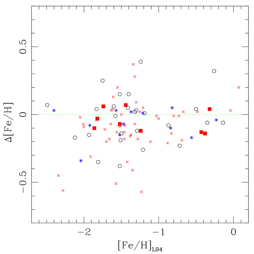
Figure 1: The difference between the [Fe/H] values of Layden (1994) and Fernley et al. (1998) is plotted as a function of each star’s metallicity from Layden (1994). Symbols indicate the number of literature sources utilized in the compilation of Fernley et al. (1998): crosses indicate $N_{src}=2$, circles mark $N_{src}=3$, asterisks mark $N_{src}=4$, and squares mark $N_{src}>4$. Stars having more sources scatter less around the mean.

Table 2: Comparing Literature Metallicities

$N_{src}$	$\overline{\Delta\rm{[Fe/H]}}$	$\sigma$	$N_{star}$	$\overline{\sigma_{L94}}$	$\overline{\sigma_{F98}}$
2	–0.096	0.200	45	0.124	0.157
3	–0.026	0.181	27	0.127	0.129
4	–0.068	0.108	12	0.135	0
$>$4	–0.047	0.080	9	0.112	0
all	–0.067	0.179	93	0.125	0.128

2.2 Interstellar Reddening from the Literature

Interstellar absorption, $A_{K}$, is a critical component of converting a star’s apparent magnitude into its absolute magnitude. In general, absorption is proportional to interstellar reddening, $E(B-V)$, and a variety of sources in the literature can yield reddening values for a given star. These sources have improved markedly since Fernley et al. (1998), who primarily used the reddening maps of Burstein & Heiles (1978), supplemented with estimates from $(V-K)$ colors for low-latitude stars. To reduce the effects of interstellar absorption, we avoided inclusion of stars with low Galactic latitude unless they were of specific astrophysical interest (metallicity, period, etc).

Schlegel, Finkbeiner & Davis (1998) used all-sky dust emission maps from the IRAS and COBE/DIRBE satellites to estimate the interstellar reddening $E(B-V)$ as a function of Galactic coordinates. We obtained an $E(B-V)$ value for every star in our sample and applied the recommended correction from the improved calibration of Schlafly & Finkbeiner (2011). Schlegel, Finkbeiner & Davis (1998) estimated the uncertainty in their reddenings to be 16% of the reddening value, which we adopted.

We also compiled $E(B-V)$ estimates from Blanco (1992), who used a metallicity-dependent relation to predict the intrinsic $(B-V)_{0}$ color at minimum light. Also, for every star in Table 1 with $V$ and $K$ magnitudes from Fernley et al. (1998), we calculated the observed $(V-K)$ color and estimated $E(B-V)$ following the procedure in Sec. 2.2 of Fernley et al. (1998). Specifically, we used Eqn. 9b of Fernley (1993) along with the period and [Fe/H] from Table 1 to estimate each star’s intrinsic $(V-K)_{0}$ color; we fit polynomials to the coefficients $c_{3}(Z)$ and $c_{6}(Z)$ in Tables 2 and 4a of Fernley (1993) to smooth the behavior of the estimates. Fernley et al. (1998) estimated the reddening uncertainty in this method to be 0.03 mag. These three values of $E(B-V)$ are presented in Table 1 as $E_{SF11}$, $E_{B92}$ and $E_{F98}$, respectively.

Figure 2 inter-compares these values. For stars with $E(B-V)_{SF11}\lesssim 0.2$ mag, both color methods follow the 1:1 correlation line with no obvious systematic offsets, so we can combine them without correction. The rms scatter of the Blanco values around the 1:1 line is 0.030 mag, while the rms is 0.034 mag for the $(V-K)$-based values. Stars with larger reddening, which tend to be close to the Galactic plane, have color-based reddenings that are smaller than predicted by the dust-maps, suggesting the dust columns may extend beyond the distance of these stars. In general, the use of three separate methods for finding the interstellar reddening and absorption enables us to detect and reject outliers, and establish a more representative mean value. In Sec. 7.4 we describe and apply a weighting scheme to combine these values into a single value for the interstellar absorption for each star; we apply a similar scheme to the stars’ photometric values as well.

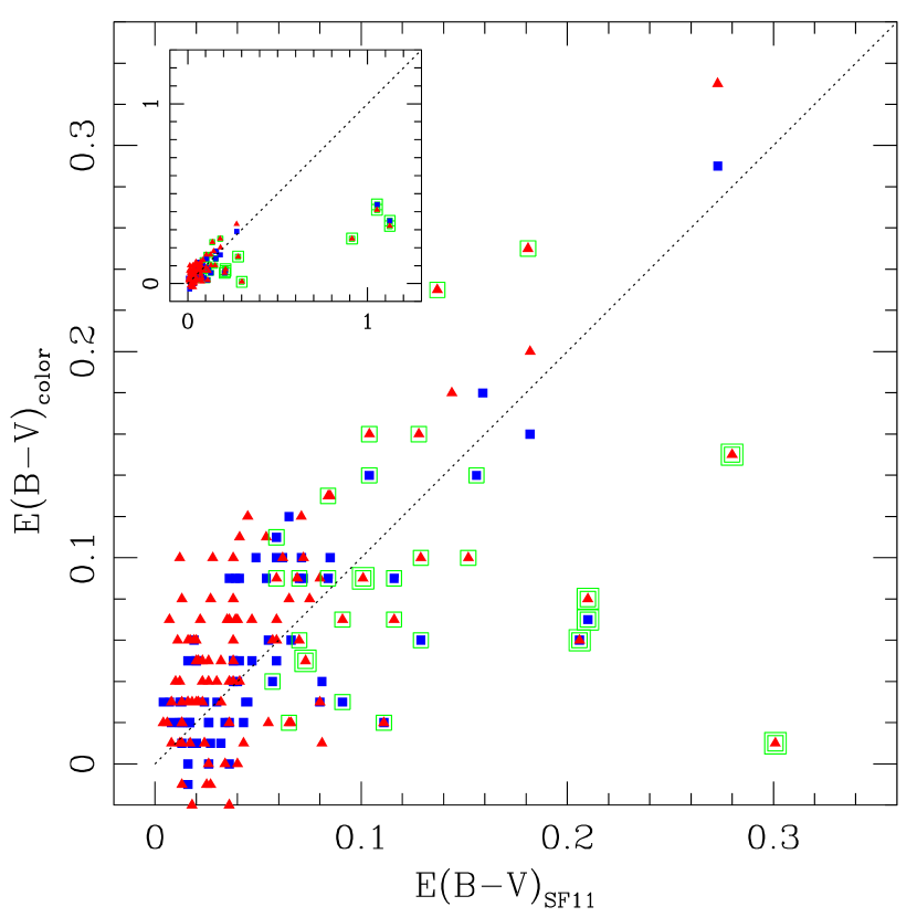
Figure 2: Interstellar reddening values based on $(B-V)$ colors (Blanco, 1992) [solid squares] and $(V-K)$ colors (Fernley et al., 1998) [solid triangles] are plotted against those from the dust map recalibration of Schlafly & Finkbeiner (2011). Stars with $|b|<20^{\circ}$ are marked with a single open square, and stars with $|b|<10^{\circ}$ are marked with a double open square. The dotted line marks the 1:1 relationship. The inset includes stars with large reddenings in our working sample of 172 stars.

2.3 Photometry from the Literature

The $K_{F98}$ column in Table 1 lists the multi-epoch $K$-band mean magnitudes available in the literature compiled by Fernley et al. (1998). Our photometry reference numbers 1–3 in this table match those of Fernley et al. (1998): reference number 1 indicates the star is among the 29 listed in Table 16 of Skillen et al. (1993) for which dozens of observations, distributed uniformly in phase, were acquired as part of previous Baade-Wessilink (BW) studies by three separate teams (a note in the Comments column cites the source of the original photometry, as identified in the notes to Table 1). The density of points in the light curves of these stars makes them the most reliable stars in our study. Reference number 2 indicates that the $K_{F98}$ value is based on the mean of a handful of photometric observations by Fernley, Skillen & Burki (1993), while #3 refers to unpublished photometry reported in Fernley et al. (1998).

The recent compilations in Table 5 of Monson et al. (2017) and Table 1 of Hajdu et al. (2018) support our literature search that found no new multi-epoch $K$-band data published since Fernley et al. (1998), with the exception of NSV 660 which was observed extensively by 2MASS in one of its calibration fields (Szabó et al., 2014). Because the light curve of this star was obtained with the 2MASS $K_{s}$ filter, we add NSV 660 to our collection of observations in Table 1. Szabó et al. (2014) included a period and estimated $[\mathrm{Fe/H}]=-1.31\pm 0.03$ dex for NSV 660 but noted the possibility of systematic uncertainties, so we adopt an uncertainty of 0.10 dex. This star has since been named LP Cet, but we retain the older name to emphasize its distinct nature from the other stars in our study.

We add to our Table 1, after the entries for the 75 stars which we observed and the entry for NSV 660, an additional 24 stars with extensive photometry from BW analyses, SW And through UU Vir. The final 47 stars in our table have lower quality $K$-band photometry from Fernley et al. (1998). We have not obtained new observations for these stars, but will explore their photometric recalibration and overall utility in Sec. 7. The recent intensity-mean $K_{s}$ values based on single-epoch photometry (Dambis, 2009; Dambis et al., 2013) are described and compared with our results and the multi-epoch photometry from Table 1 in Sec. 7.

Stars known to exhibit the Blazhko effect are noted in the comments column of Table 1. Jurcsik et al. (2018) showed that a star exhibiting a well-defined Blazhko cycle in the $I$-band shows related brightness variations in the $K$-band of $\sim$0.1 mag, less than half the star’s Blazhko cycle $I$-band amplitude (see their Figure 3). While this effect is small, observations made at different points in a star’s Blazhko cycle could lead to a biased estimate of the star’s intensity-mean magnitude, so we have intentionally avoided observing Blazhko stars unless they are of other astrophysical interest.

2.4 Characterizing the Sample

Figure 3 plots period versus metallicity for the stars in Table 1. The identification of stars as fundamental or first-overtone pulsators, RRab or RRc respectively, was taken from the literature and was based on the stars’ periods, amplitudes, and light curve shapes. The well-known trend between period and metallicity is apparent, as is the separation between RRab and RRc. We selected our targets (the first 75 stars listed in Table 1) to complement the period-metallicity distribution of the 30 existing high-quality light curves produced in the course of past BW analyses.

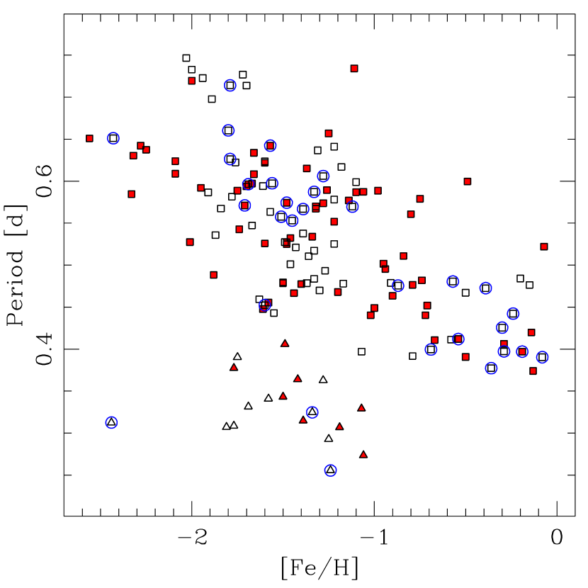
Figure 3: Period is plotted against [Fe/H] for the 146 RRL stars from Table 1, with squares and triangles marking ab-type and c-type RRL, respectively. Stars we observed are filled, and stars which have been observed as part of previous Baade-Wesselink studies are circled.

We used the proper motions from the Gaia DR2, and radial velocity data from Fernley et al. (1998) and Layden et al. (1996), in the “space motion” solution method described in Layden (1995) to obtain the three-dimensional velocities of the stars in our working database. Figure 4 shows these $UVW$ motions plotted against metallicity. The stars with higher metallicities have the smaller velocity dispersions and Sun-like Galactic rotation commonly found for the Galactic thick disk, whereas the more metal poor stars have the broad velocity dispersions and net rotation that lags the Sun by $\sim$200 km s^-1 typical of stars in the Galactic halo (Layden, 1995). The transition between these kinematic populations appears to be at [Fe/H] $\approx-0.9$ dex on our metallicity scale. Some of the stars with [Fe/H] $<-0.9$ that have low velocity dispersions and $V\approx 0$ km s^-1 may be members of the metal-weak thick disk (Layden, 1995; Dambis, 2009). We used an earlier version of this plot when selecting stars for our observation program to ensure a good distribution of stars around the disk-halo boundary, so that our data would be sensitive to any luminosity discontinuity between these two kinematic populations.

In total, Table 1 contains 147 stars that make up our initial data set, originally designed as a target list for SIM-PQ but now useful in the era of Gaia.

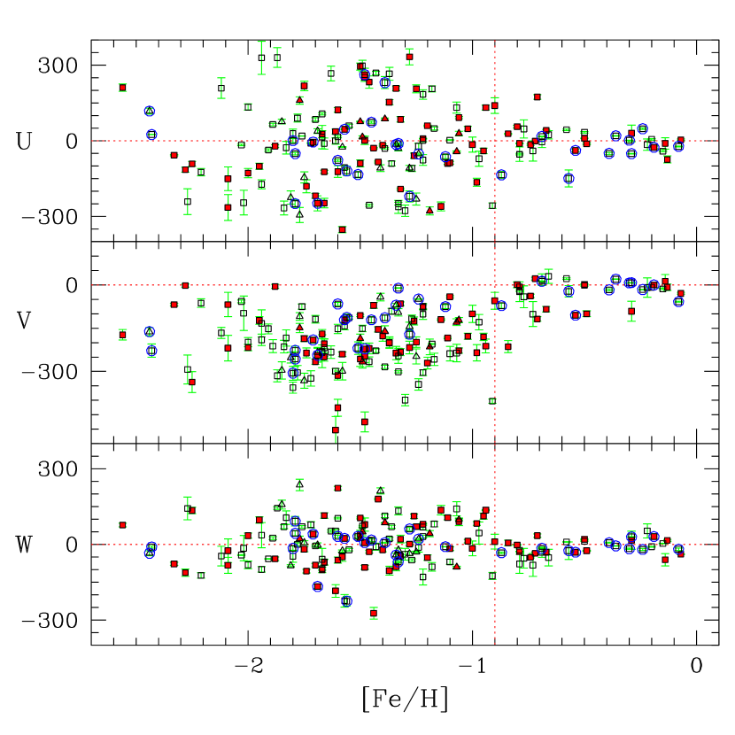
Figure 4: The $UVW$ space velocities, in units of km s^-1, are plotted against metallicity for RRL in our database, showing (top) the $U$ velocity component, directed towards and away from the Galactic center; (center) the $V$ velocity, along the direction of Galactic rotation; (bottom) the $W$ component, directed perpendicular to the Galactic plane. Squares and triangles mark ab- and c-type RRL. Filled symbols mark stars we observed in the $K_{s}$-band, while circles mark stars with high-quality BW photometry.

3 Observations

Since our target stars shown in Table 1 are spread across the entire sky, we obtained images of these RRL using two different sets of equipment. In the Southern hemisphere, we used the 1.3-m telescope of the Small and Medium Aperture Research Telescope System (SMARTS) consortium located on Cerro Tololo in Chile in queue-scheduled mode during 229 nights between 2004 January 27 and 2005 January 30. We used the ANDICAM instrument to obtain images simultaneously through the $K_{s}$ and Cousins $I_{C}$ filters using different optical paths and detectors within the instrument. In this work, we used the $I_{C}$ images only for differential photometry that enables us to determine the phases of our $K_{s}$ images; a full analysis of the optical images will be reported in a forthcoming paper (Layden et al., 2020). The infrared array was a Rockwell HgCdTe device with 18-micron pixels, operated with $2\times 2$ pixel binning to give images with a $2.4\times 2.4$ arcmin field of view and 0.27 arcsec pixel^-1 scale. The north-east quadrant of the array was not functional so our images have an L-shaped field of view. Exposure times of individual images were typically 6-20 s at each of five dither positions. As part of the queue-observing process, calibration frames were obtained at regular intervals and these were applied to the raw images using standard procedures. For a given star, the individual dithered images from a particular visit were combined to produce a single $K$-band image for that epoch. The median seeing in this data set was 0.8 arcsec fwhm; the best and worst seeing values were 0.6 and 1.8 arcsec, respectively.

In the Northern hemisphere, we obtained images using the McGraw-Hill 1.3-m telescope at the Michigan-Dartmouth-MIT (MDM) Observatory on Kitt Peak in Arizona using the TIFKAM infrared imager during observing runs on 2006 June 9-25 and on 2007 June 23 through July 5. We operated the telescope at $f/7.6$ so the $1024\times 1024$ HgCdTe array yielded images with a $6.6\times 6.6$ arcmin field of view and 0.38 arcsec pixels. Images of most target stars involved a sequence of ten 10- or 20-s exposures through the $K_{s}$-band filter, coadded on the array. Typically, each visit to a star involved four such images, slightly dithered between exposures to shift the stars onto different sets of pixels. These images were dark-subtracted and flat-fielded using dome flats, and the four images of each target star where shifted and combined using bad-pixel rejection into a single image per visit. Typical seeing on the MDM images was 1.6 arcsec fwhm ($\sigma=0.2$ arcsec).

For both the Northern and Southern observing campaigns, we planned the observing of each star using its known period to obtain phase coverage that was as uniform as possible. We aimed to get twenty observations per star for the southern, SMARTS targets, and owing to the more constrained observing time in the north, ten observations per star observed from MDM Observatory. In practice, weather and timing constraints sometimes affected our ability to attain these goals: the median number of observations per star that we secured were 17 using SMARTS and ten using the MDM facilities.

4 Photometry and Calibration

The standard approach to variable star photometry is to obtain contemporaneous photometry in two or more filters so that instantaneous colors can be obtained that enable determination of the magnitude in each bandpass. Because we required only $K$-band photometry, and to maximize efficiency during our limited observing runs, we employed a different approach using only the $K_{S}$ filter to perform differential photometry with respect to on-frame comparison stars of known magnitude and color. We describe the details of the method below and discuss its effect on our photometry in Sec. 6.

Because our target RR Lyrae stars were selected to be of low-reddening, hence far from the Galactic plane, crowding was rarely an issue, and we performed aperture photometry using the implementation of DAOPHOT (Stetson, 1987) in IRAF to measure instrumental photometry of the variable and comparison stars on each image. On most images, we chose a stellar aperture with a diameter 3.5 times the typical seeing.

We selected comparison stars in the field of view of each variable star and retrieved their photometry from the 2MASS Point Source Catalog (Skrutskie et al., 2006). We selected stars of similar brightness and color to the variable, finding between one and twelve (typically four) suitable comparison stars in the various fields of view (the smaller, L-shaped field of view of the SMARTS images tended to permit fewer comparison stars, typically two). We assumed that our instrumental magnitudes, $k$, would be related to the standard 2MASS magnitudes, $K_{s}$ by a function with the form

$$k-K_{s}=c_{0}+c_{1}(J-K_{s}),$$ (1)

where $(J-K_{s})$ is the standard color from the 2MASS list. We performed least-squares regressions on data for comparison stars from a number of the richer fields to determine the values of the coefficients $c_{0}$ and $c_{1}$. While the zero-point $c_{0}$ varied from image to image as the airmass and transparency varied, the color-term $c_{1}$ tended to remain stable, so we averaged the results to obtain $c_{1}=+0.024\pm 0.015$ from 21 fields for the MDM data. This approach was complicated for the SMARTS data by the smaller number of on-frame comparison stars; we obtained $c_{1}=-0.002\pm 0.051$ from 14 fields, a value consistent with the experience of the SMARTS technical team, who found found no discernible color-term using this equipment (Pogge, 2018). Systematic effects resulting from these color-terms are addressed in Sec. 6.

On each image, we used the instrumental magnitude of the variable star, $k_{v}$ and one of the comparison stars, $k_{c}$, along with the 2MASS magnitude and color of the comparison star ($K_{c}$ and $(J-K)_{c}$, respectively) to estimate the standard magnitude of the variable star, $K_{v}$, differentially using the equation

$$K_{v}=K_{c}+k_{v}-k_{c}-c_{1}[(J-K)_{v}-(J-K)_{c}].$$ (2)

The 2MASS data includes values for $K_{v}$ and $(J-K)_{v}$, taken at a single epoch for each variable star. We used the latter to calibrate our differential photometry for each variable star using Eqn. 2. In reality, the surface temperature and hence the color of the variable changes as the star pulsates; the $J-K$ color range is $\sim$0.25 mag for a typical ab-type RRL, and $\sim$0.1 mag for a typical c-type (Skillen et al., 1993). We discuss in Sec. 6 how this simplification affects our photometric calibration, and we describe how the 2MASS values for the RRL and a check star are used to test our calibrated light curve for each variable star.

On each image, we used Eqn. 2 to calculate $K_{v}$ for the variable from each available comparison star, leading to $N_{\rm comp}$ separate estimates of the RR Lyrae’s brightness. We took the mean of these $N_{\rm comp}$ values, giving double-weight to stars that were bright or particularly close in color to the variable. The standard error of the mean of these $N_{\rm comp}$ values, $\sigma_{m}$, provides an uncertainty estimate for the mean value, $K_{s}$, for this observation. These data are presented in Table 3 for each image, where the columns include the star name, heliocentric Julian Date of the observation, the pulsation phase (see Sec. 5), the airmass of the star at the time of observation, and the observatory from which the image was acquired. The last column provides an integer code describing the quality of the variable star’s image profile estimated by visual inspection of each image: $Q=2$ indicates a normal, high quality profile, while $Q=1$ flags a lower quality profile in which trailing due to telescope drift, interference from a flat-fielding artifact, or proximity to the edge of the fully-calibrated region of the image makes the $K_{s}$ value somewhat less certain than its $\sigma_{m}$ value may suggest. Of the 1060 photometric measurements reported in Table 3, only 62 have low quality.

Table 3: Time-Series Photometry of the Variable Stars

Star	HJD	$\phi$	$K_{s}$	$\sigma_{m}$	$N_{\rm comp}$	Airmass	Obs	$Q$
DM And	2453898.9050	0.717	10.616	0.006	5	1.48	2	2
DM And	2453898.9504	0.789	10.672	0.010	5	1.21	2	2
$\cdots$	$\cdots$	$\cdots$	$\cdots$	$\cdots$	$\cdots$	$\cdots$	$\cdots$	$\cdots$
DM And	2454285.8761	0.578	10.531	0.006	6	1.29	2	2
WY Ant	2453035.7338	0.388	9.535	0.020	1	1.02	1	2
WY Ant	2453038.6888	0.533	9.580	0.020	1	1.08	1	2
$\cdots$	$\cdots$	$\cdots$	$\cdots$	$\cdots$	$\cdots$	$\cdots$	$\cdots$	$\cdots$
AV Vir	2453906.7785	0.831	10.710	0.004	3	1.82	2	2

Note. — (This table is available in its entirety in machine-readable form.)

5 Template Fitting

Our primary goal is to obtain the intensity-mean $K_{s}$ magnitude of each star in Table 1. To accomplish this goal, we folded the observed data from Table 3 for a given star with the star’s known period, and fit the resulting phased light curve with a sequence of light curve templates. Following Layden (1998), the fitting adjusted each template by shifting it vertically to obtain a magnitude zero-point, shifting it horizontally to match the phase of the observations, and stretching it vertically to obtain the amplitude, using the downhill simplex method (Press et al., 1986) to minimize the error-weighted $\chi^{2}$ between the observations and the template. We did a three-parameter fit for each template in the sequence, inspected visually the four best fits, and in the vast majority of cases we adopted the fitted template with the smallest $\chi^{2}$.

In addition, we fit our observations with both of the periods shown in Table 1 and inspected the resulting phased light curves in both $K_{s}$ and $V$ or $I$. In cases where the VSX period produced light curves with less scatter, or when they were indistinguishable, we adopted the VSX period: it is reported in Table 4 along with the reference code 1. In cases where the period from Fernley et al. (1998) was preferable, we adopted it and report it in Table 4 with reference code 2. For four stars, neither period adequately phased the observations, so we obtained an improved period using our optical data (reference code 3; see details in the Appendix). We also include in Table 4 an epoch associated with each star’s maximum in optical brightness.

5.1 Templates in $K$

Because the light curve shape is a strong function of wavelength, we require templates suited to the infrared. Jones et al. (1996) developed template RRL light curves from observed $K$-band observations of 17 ab-type and four c-type stars (see their Table 3) by fitting Fourier series to the observed light curves after grouping them by $B$-band amplitude, and hence light curve shape (see their Figure 1). We used their Fourier coefficients (see their Table 4) to construct templates, named “ab1” thorough “ab4” and “c,” sampled at intervals of 0.02 phase units yielding 51 phase points. We derived an additional template, named “ab5,” by fitting a smooth curve to the data in their Figure 1f in order to capture the light curve shape with the sharpest peak.

We shifted these templates in phase so that the reference phase, defined by the sharp minima in the RRab light curves, fell at the phases shown in Figure 1 of Jones et al. (1996) that were based on the stars’ optical ephemerides (also see their Figure 2) rather than at $\phi=0$ as defined by the Fourier coefficients shown in Table 4 of Jones et al. (1996). This has the advantage that when the template is fitted to observed $K_{s}$ data, $\phi=0$ should correspond to the maximum brightness in the $V$-band.

Jones et al. (1996) discussed a use of their templates in which the ephemeris of an RRL is known but only 1-2 $K$-band observations have been obtained. They developed phase-amplitude (their Fig. 2 and Eqn. 6) and amplitude-amplitude (their Fig. 3 and Eqns. 7-9) relations that would enable a star’s $B$-amplitude value to predict the star’s phase and $K$-amplitude, so the appropriate template could be matched to the $K$-band observation to obtain the star’s mean $K$-band magnitude. We chose to gather more than 1-2 observations per star for several reasons. Our chief concern was the degree of scatter and bifurcation of their $B$- versus $K$-amplitude relation, which could result in the use of the wrong amplitude for a given star. Second, each template in Jones et al. (1996) is derived from the observed light curves of 3-7 individual stars (see their Table 3); these stars may not represent the complete range of RRL light curve shapes as seen across a wider range of metallicities and stellar populations (for example, see the cases of RV Cap and RX Col below). Finally, by obtaining more data points and fitting a template, we reduced the effect of random photometric errors in each observation. However, as described below, we did perform such one-parameter fits for several stars whose observations were insufficient for our preferred three-parameter fitting approach.

5.2 Fitting SMARTS data

Most of the southern stars observed with SMARTS were visited enough times so that one or more points were obtained during a star’s steep brightness rise from minimum to maximum light. This provided a good constraint on the horizontal, phase-shift component of the three-parameter fit for that star. We tested whether the result was correctly phased by plotting the contemporaneous $I$-band photometry for each star using the same period and epoch as the $K$-band data, and in almost every case, the maximum in the $I$-band light curve occurred at a phase of 0.0 as expected for a correctly-phased $K$-band light curve. Figure 5 shows an example of one fit. Of the 42 stars observed with SMARTS, only two (RX Cet and W Tuc) failed to produce reliable three-parameter fits; their cases are described below and in the Appendix.

We computed the intensity-mean $K_{s}$ magnitude for each star from the individual data points and from the best-fit template. For stars with light curves that were well-sampled in phase, they differed by only a few millimag, so we averaged the values; in under-sampled cases we used the result from the template fit alone. In most cases, we determined the light curve extrema, $K_{max}$ and $K_{min}$, from the best-fit template, since the scatter of individual data points can lead to spuriously large amplitudes. The weighted standard deviation of a star’s points around the best-fit template, $\sigma_{fit}$, is a useful measure of the quality of the fit. This scatter is due to factors such as the photometric uncertainty in each observed data point (which is related to signal strength, sky noise, and errors in image processing), the horizontal scatter in points due to an error or change in a star’s period (in most cases this was negligibly small because of the high precision of our periods and short interval of observation epochs), and any cycle-to-cycle modulation of the RRL light curve due to intrinsic sources like the Blazhko effect. For the forty stars with three-parameter fits, the median value of $\sigma_{fit}$ was 0.027 mag.

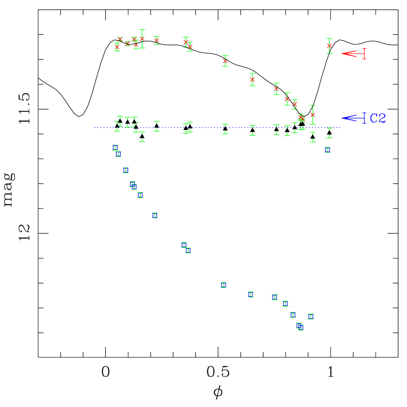
Figure 5: The phased light curves of BP Pav: crosses show our SMARTS $K_{s}$ magnitudes and the solid curve is the template fit to them. The triangles are our $K_{s}$ magnitudes of the comparison star C2, and the dotted line shows their median magnitude. The horizontal arrows show the 2MASS $K_{s}$ magnitude of BP Pav (upper) and of C2 (lower), and the error bars show their 2MASS uncertainties. The open squares show contemporaneous $I$-band magnitudes of BP Pav, shifted vertically for convenience of display; these data peak at a phase of 0.0 confirming that the $K_{s}$ data were correctly phased by the three-parameter template fit (see Sec. 5).

5.3 Fitting MDM data

Of the 34 northern stars observed with MDM, 28 had enough data points with adequate phase distribution to constrain reliable three-parameter light curve fits. In general, these stars had a larger number of on-field comparison stars than the SMARTS data, and the uncertainties in their individual $K_{s}$ magnitudes were smaller, resulting in a median $\sigma_{fit}$ of 0.013 mag. These stars did not have contemporaneous optical data with which to confirm their phases, but for each star we have uncalibrated $V$ or $I$ time-series photometry from the 0.5-m telescope at Bowling Green State University (BGSU) in Ohio, which will be presented in a forthcoming paper (Layden et al., 2020). These optical data were often acquired several years before or after the MDM data, so small errors or changes in a star’s period could result in a phase offset between the optical and $K_{s}$ data. We therefore fit the light curve with both the Fernley et al. (1998) and VSX periods and adopted the period giving the tightest light curves and the maximum at optical light closest to $\phi=0$. While the choice of periods made little difference in the distribution of $K_{s}$ points in phase (the MDM data were taken over a period of time – days or up to one year – that is short compared with the time between when the MDM and BGSU data were taken), in some cases it resulted in a small phase shift and consequent selection of a different best-fit template. The difference in the resulting mean $K_{s}$ magnitude was always insignificant (mean $=-0.001\pm 0.003$ mag). As a check on the size of phase offsets that might occur during the time elapsed between the acquisition of the optical and infrared images, we computed the number of cycles elapsed using the adopted period, and one computed using a reasonable offset in that period (based on the published precision of the adopted period). Only two stars had unacceptably-large cycle-count discrepancies (XZ Dra and RV UMa; see the Appendix for details), while the rest had discrepancies smaller than $\sim$0.02 cycles. For all of the 28 stars with three-parameter fits, visual inspection of the light curves led us to a high confidence in the quality of the fits. The mean and extreme $K_{s}$ values for these 28 stars were calculated as described in the previous subsection for the SMARTS stars.

5.4 Other Fits

For six of the MDM stars and two of the SMARTS stars, the $K$-band observations were insufficient in number or phase distribution to adequately constrain the fits. For each of these stars, we made a preliminary phased light curve using an arbitrary epoch and the known period for both the $K$-band and optical data, and determined a phase shift that would bring the peak of the optical light curve to $\phi=0$, thereby phasing correctly the $K_{s}$ data. For cases where the Fernley et al. (1998) and VSX periods produced significantly different light curves, we again adopted the period yielding the tightest light curve and the optical-light maximum closest to $\phi=0$. For one star, YZ Cap, constraining the phase this way was sufficient to obtain an acceptable two-parameter fit which solved for the star’s amplitude and zero-point (see the Appendix for details).

For the seven remaining stars, there were too few points in the critical phases around the deep, brief minima to adequately constrain the amplitude of the fit. Here, we reverted to the original template fitting scheme outlined in Jones et al. (1996). We obtained a star’s optical amplitude from the literature, often $B$-band data from Bookmeyer et al. (1977), and used Eqn. 7 of Jones et al. (1996) to predict the star’s $K$-band amplitude. We also used the star’s $B$-band amplitude to select a template from the groupings in Figure 1 of Jones et al. (1996), which demonstrates the correlation between amplitude and light curve shape. We then performed a one-parameter fit using this template, amplitude, and phase-shift in order to find the zero-point that gave the best fit between the observations and scaled template. Figure 6 shows the fit for AA Aqr, in which $I$-band photometry from BGSU was used to constrain the phase of the MDM $K_{s}$ photometry. For the stars utilizing one- and two-parameter fits, mean and extreme $K_{s}$ magnitudes were obtained from the best-fit template alone, and details of the fitting procedures are provided in the Appendix.

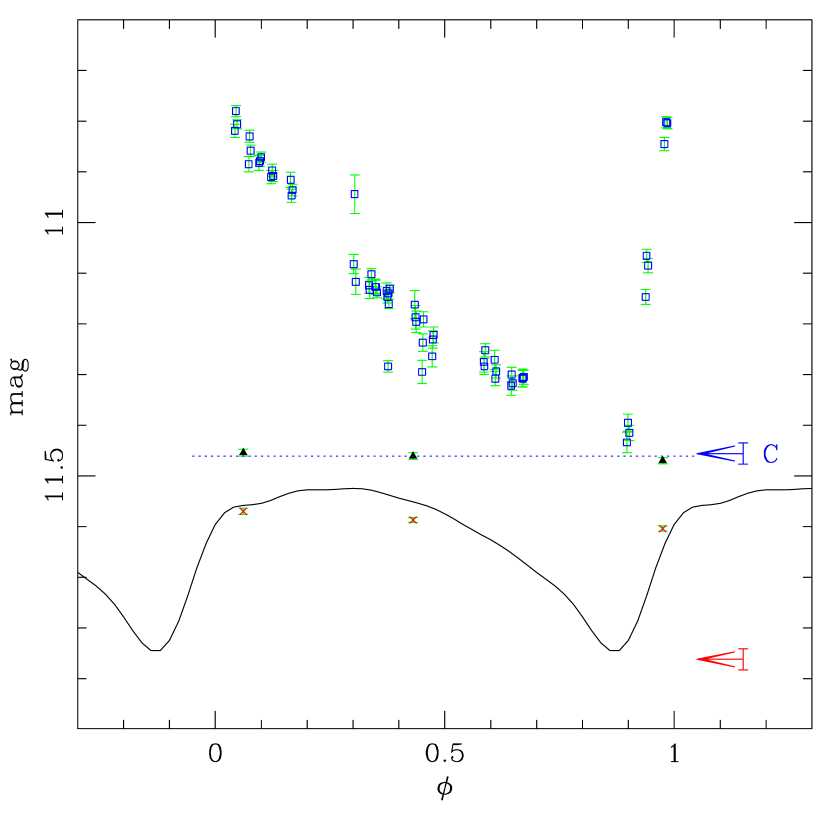
Figure 6: The phased light curves of AA Aqr. The symbols are as in Figure 5. Comparison star “C” is shown as a non-variable check star. The $I$-band observations were obtained at BGSU less than one year before the MDM $K_{s}$ observations, and their maximum was shifted to $\phi=0$ to establish the phases of the $I$ and $K_{s}$ data. The template “ab2” was scaled to an amplitude of $\Delta K=0.32$ mag based on the $V$-band amplitude of Munari, Henden & Frigo (2014), and shifted vertically using a one-parameter fit.

5.5 Resulting Photometry

Figure 7 shows our observed $K_{s}$ data for forty RRL observed with SMARTS and their template fits, while Figure 8 shows the data and fits for 34 stars observed at MDM. Table 4 lists the intensity-mean magnitude, $\langle K_{s}\rangle$, for each star, along with its extrema $K_{max}$ and $K_{min}$, the number of observations $N_{obs}$, $\sigma_{fit}$ and the name of the best-fitting template, and the number of comparison stars $N_{comp}$ used to calibrate the differential photometry via Eqn. 2.

One star, BX Dra, was listed by Fernley et al. (1998) as an RRab star and was thus included in Table 1, but optical observations have shown it to be a contact eclipsing binary system (see Park et al. (2013) and references therein). Our $K_{s}$-band light curve shown in Figure 8 is consistent with this conclusion and we do not consider BX Dra further in the following analysis.

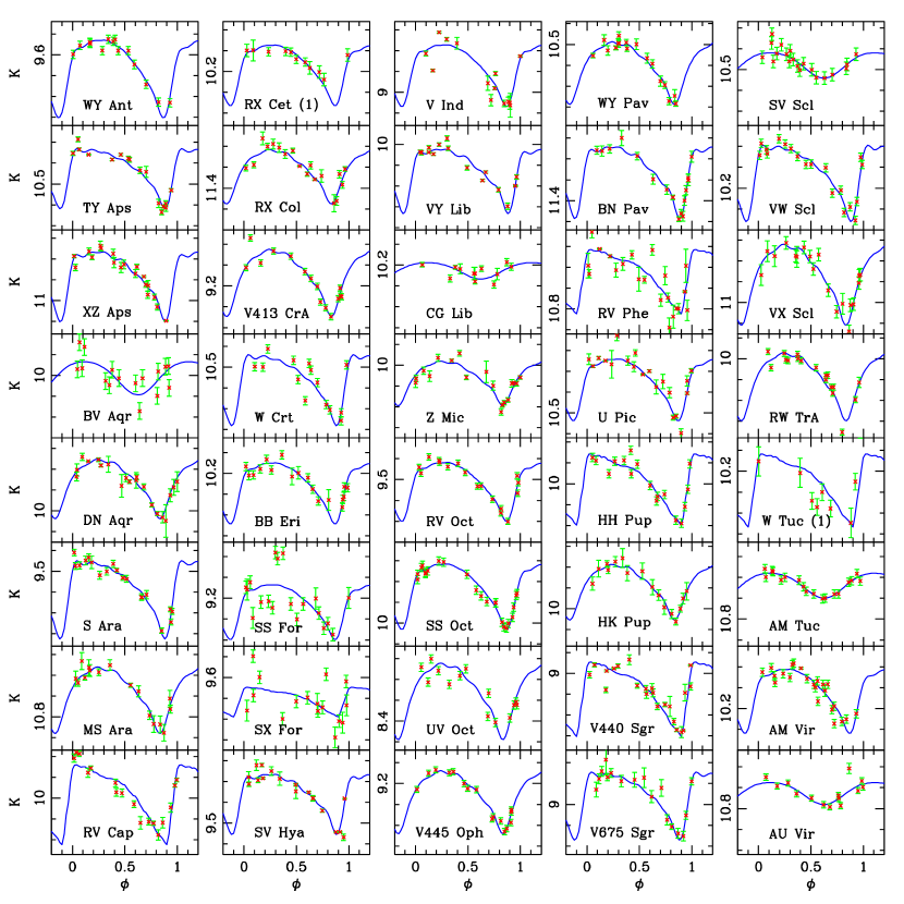
Figure 7: The phased $K_{s}$ light curves of forty RRL observed with SMARTS. All the templates were fitted using a three-parameter fit unless noted by “(1)” which indicates a one-parameter fit. Each panel has a vertical range of 0.5 mag.

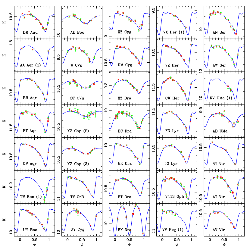
Figure 8: The phased $K_{s}$ light curves of 34 stars observed at MDM. Circles indicate 2006 data and crosses mark 2007 data. All the templates were fitted using a three-parameter fit unless noted by “(1)” or “(2)” indicating a one- or two-parameter fit. Each panel has a vertical range of 0.5 mag. The star YZ Cap was also observed with SMARTS; this light curve is indicated by the “(S).” The star BX Dra was confirmed to be an EW-type contact binary system.

Table 4: Final Photometry of the Variable Stars

Star	Obs	$N_{comp}$	$N_{obs}$	Period	Ref	Epoch	$\langle K_{s}\rangle$	$K_{max}$	$K_{min}$	$N_{par}$	Temp	$\sigma_{fit}$	$\sigma_{z}$	$\sigma_{c}$	$\sigma_{K}$
DM And	2	6	18	0.630389	2	3898.45301	10.543	10.46	10.73	3	ab2	0.016	0.007	0.001	0.008
WY Ant	1	1	14	0.574312	2	3035.51097	9.639	9.53	9.90	3	ab2	0.022	0.032	0.005	0.033
$\cdots$	$\cdots$	$\cdots$	$\cdots$	$\cdots$	$\cdots$	$\cdots$	$\cdots$	$\cdots$	$\cdots$	$\cdots$	$\cdots$	$\cdots$
AU Vir	1	1	14	0.3432307	1	3077.67294	10.717	10.67	10.78	3	c	0.026	0.030	0.019	0.036
AV Vir	2	3	8	0.6569073	1	3898.34958	10.548	10.47	10.74	3	ab2	0.013	0.012	0.004	0.014
NSV 660	3	$\cdots$	2969	0.636985	1	0659.80021	13.987	13.90	14.20	3	ab2	0.074	$\cdots$	$\cdots$	0.02

Note. — (This table is available in its entirety in machine-readable form.)

6 Photometric Uncertainties

It is important to obtain a reliable estimate of the uncertainty in the measured intensity-mean $\langle K_{s}\rangle$ magnitude for each star in our sample. There are several sources of uncertainty. First is the uncertainty in the vertical, zero-point level of our fitted template. We noted earlier that $\sigma_{fit}$ describes the point-to-point scatter of the observed points around the best fit, and we adopt a value based on the standard deviation of the mean as the uncertainty in the zero-point of the fitted template, $\sigma_{t}=\sigma_{fit}~{}N_{obs}^{-0.5}$.

The second source of uncertainty is that of the 2MASS magnitude of each comparison star, $\sigma_{i}$. Typically, $\sigma_{i}\approx 0.02$ mag, increasing for fainter stars. These errors are mainly random, due to errors in point-spread-function fitting, read noise, flat-field noise, etc. (Skrutskie et al., 2006), so for an RRL with multiple comparison stars, we combined the errors via $\sigma_{z}=(\Sigma~{}\sigma_{i}^{-2})^{-0.5}$ to obtain a single estimate of the uncertainty in the external calibration. The value of $\sigma_{z}$ for each star is listed in Table 4.

The third uncertainty source is the uncertainty in our color term, $c_{1}$, used to account for the color difference between variable and comparison stars in Eqn. 2. Across our sample, the median 2MASS color of the RRL was $(J-K_{s})=0.30$ mag with a standard deviation of 0.07 mag, while the median comparison star color was 0.53 mag with a broader standard deviation of 0.20 mag. For each variable-comparison star pair, we computed the color difference $\Delta(J-K_{s})$ between the two stars’ 2MASS colors, and calculated the resulting systematic uncertainty in the star’s mean $K_{s}$ magnitude as $\sigma_{c}=\sigma_{c1}\times\Delta(J-K_{s})$, where $\sigma_{c1}=0.051$ mag for the SMARTS data and 0.015 mag for the MDM data. For each variable with multiple comparison stars, we computed the weighted mean of the individual $\sigma_{c}$ values, reported for each RRL in Table 4. The median values of $\sigma_{c}$ were 0.015 and 0.004 for the SMARTS and MDM fields, respectively.

An additional source of error in our $K$-band light curves originates with our non-standard procedure for calibrating the differential photometry, i.e., using only one filter rather than two filters, which would enable the calculation of a variable star’s instantaneous color. In Eqn. 2, we used for $(J-K_{s})_{v}$ the 2MASS single-epoch color of the RRL rather than its instantaneous color. We therefore made an error in all the magnitudes for a given star. This error can be estimated as $\sigma_{n}=c_{1}\times\sigma_{jk}$, where $\sigma_{jk}$ is the standard deviation of the $(J-K_{s})$ values a star experiences over the course of its pulsation cycle. We determined $\sigma_{jk}$ for each of the four ab-type RRL (obtaining an average value of 0.073 mag) and for the one c-type RRL (0.045 mag) in Skillen et al. (1993). Thus, we expect that each ab-type RRL observed with MDM ($c_{1}=+0.024$) should have an additional component to its uncertainty of $\sigma_{n}=0.002$ mag, and each c-type RRL an added uncertainty of 0.001 mag. The small color term for SMARTS observations ($c_{1}=-0.002$ mag) makes this component of the uncertainty negligibly small.

We calculated each of these four sources of uncertainty ($\sigma_{t}$, $\sigma_{z}$, $\sigma_{c}$, and $\sigma_{n}$) for each star and added them in quadrature to obtain an overall systematic uncertainty in the intensity-mean $\langle K_{s}\rangle$ magnitude for that star, $\sigma_{K}$, whose values are listed in Table 4. The relative sizes of these uncertainties gives a sense of the relative strengths and weaknesses of each component of the procedure for each star, and across all the stars in our sample. For stars observed with SMARTS, the median value of $\sigma_{K}$ was 0.029 mag, while it was 0.013 mag for the MDM stars. Based on the scatter of observed points around the best fit templates, we estimate the uncertainty in the extrema values $K_{max}$ and $K_{min}$ in Table 4 to be about 0.02 mag for a typical star, though stars with larger values of $\sigma_{fit}$ are expected to have larger uncertainties in their extrema.

We performed two tests on our photometry of each star to identify potential problems with our procedure. First, for each RRL we selected one comparison star and processed it with our variable star software, using the remaining $N_{comp}-1$ comparison stars to determine its time-series differential photometry. In all cases, like those shown in Figures 5 and 6 for comparison stars “C2” and “C” respectively, we obtained a flat run of magnitude with phase and a scatter comparable in size to the uncertainty estimates from our individual photometric measurements. For example, the rms scatter of the points for the comparison star C2 in Figure 5 was 0.018 mag, while the mean uncertainty was 0.020 mag for this SMARTS star; for the check star in Figure 6 the values were 0.008 and 0.005 mag, respectively (MDM); and for the better-sampled MDM star FN Lyr, the values were 0.007 and 0.005 mag. Furthermore, the median of our $K_{s}$ magnitude estimates for each check star were statistically consistent with the star’s 2MASS $K_{s}$ mag measurement, as shown by the labeled arrows in Figures 5 and 6.

The second consistency test was to plot the single-epoch $K_{s}$ magnitude of the RRL from 2MASS on each star’s light curve, and visually check whether it fell between the $K_{max}$ and $K_{min}$ range of the fitted template. For almost all our RRL, this was the case (for example, see Figure 5). For three stars, the 2MASS magnitude was formally outside the template range, but by an amount consistent with the uncertainty in the 2MASS magnitude (see Figure 6). Only for the stars DM Cyg and SX For was the 2MASS magnitude significantly outside the template range (by 0.07 and 0.16 mag, respectively). We recommend independent photometry of these stars.

7 Photometric Comparisons

We have one star in common between the southern SMARTS and northern MDM data sets, YZ Cap. Unfortunately, this provides a poor comparison because the SMARTS data for this c-type RRL had a fairly large scatter around the best template (see Figure 8), $\sigma_{fit}=0.026$ mag, and had only two comparison stars that were somewhat faint, leading to a large uncertainty in the intensity-mean magnitude, $\langle K_{s}\rangle=10.293\pm 0.033$ mag. The MDM data had more comparison stars and a smaller overall uncertainty, yielding $\langle K_{s}\rangle=10.359\pm 0.012$ mag. The difference of $0.066\pm 0.035$ ($1.9\sigma$) hints that the SMARTS data may be systematically brighter than the MDM data, though the evidence is not compelling and there is little fundamental reason to think our differential photometry should suffer a systematic offset.

7.1 Compiled Photometry

In order to compare our photometry with existing work from the literature, we assembled the available data in Table 5. The second column contains the intensity-mean magnitudes derived from the BW studies noted in Table 1. Both Monson et al. (2017) and Hajdu et al. (2018) (see their Table 1) emphasized that most archival data were obtained using a mixture of photometric systems which may be less uniform than our $K_{s}$ data. In their Table 5, Monson et al. (2017) provided intensity-mean values recalibrated to the 2MASS photometric system for twenty of the BW RRL in our study, including the star RR Lyrae itself. These data should be consistent with our $K_{s}$ photometry, and appear in the second column of Table 5 labeled $K_{BW}^{\prime}$, where the prime indicates the original magnitudes have been transformed to the 2MASS system.

For ten additional BW stars, we used the relations of Carpenter (2003), several of which appear as Eqns. 4-6 of Monson et al. (2017), to transform the published intensity-mean magnitudes onto the $K_{s}$ system, as shown in Table 6. In this table, the second column contains the intensity-mean $K$ magnitude listed in the paper cited in column three, and the fourth column identifies the equation used in the transformation. The transformed values for these ten stars also appear in the second column of Table 5 (note that VY Ser was observed by two separate teams; we averaged the transformed results to achieve the value shown in Table 5). For all 30 BW stars we adopt photometric uncertainties of 0.009 mag following Monson et al. (2017). For convenience, columns 3–4 of Table 5 repeat our $\langle K_{s}\rangle$ and $\sigma_{K}$ values from Table 4.

Table 5: Combined Photometry and Interstellar Absorption

Star	$K_{BW}^{\prime}$	$\langle K_{s}\rangle$	$\sigma_{K_{s}}$	$K_{F98}^{\prime}$	$\sigma_{F98}$	$K_{D13}$	$\sigma_{D13}$	CodeK	$\bar{\langle K\rangle}$	$\sigma_{\bar{K}}$	Flag	$A_{K}$	$\sigma_{A}$	CodeA
SW And	8.511	$\cdots$	$\cdots$	$\cdots$	$\cdots$	8.509	0.034	1001	8.511	0.009	0	0.017	0.003	111
XX And	$\cdots$	$\cdots$	$\cdots$	9.491	0.044	9.411	0.035	0021	9.442	0.027	0	0.013	0.003	111
AT And	$\cdots$	$\cdots$	$\cdots$	9.041	0.044	9.090	0.036	0021	9.070	0.028	0	0.044	0.005	111
DM And	$\cdots$	10.543	0.008	$\cdots$	$\cdots$	10.575	0.038	0201	10.544	0.008	0	0.029	0.005	100
$\cdots$	$\cdots$	$\cdots$	$\cdots$	$\cdots$	$\cdots$	$\cdots$	$\cdots$	$\cdots$	$\cdots$	$\cdots$	$\cdots$	$\cdots$	$\cdots$	$\cdots$
AV Vir	$\cdots$	10.548	0.014	10.611	0.044	10.566	0.037	0221	10.555	0.013	0	0.008	0.003	101
BN Vul	$\cdots$	$\cdots$	$\cdots$	8.791	0.044	8.665	0.033	0021	8.710	0.026	0	0.153	0.008	911
NSV 660	$\cdots$	13.987	0.020	$\cdots$	$\cdots$	$\cdots$	$\cdots$	0400	13.987	0.020	0	0.011	0.004	100

Note. — (This table is available in its entirety in machine-readable form.)

Table 6: Additional BW Photometry

Star	$K_{BW}$	Ref	Equation
RS Boo	9.445	bw24	Monson et al. (2017) Eqn. 4 (CIT)
UU Cet	10.850	bw35	Carpenter (2003) Sec. c (ESO)
SW Dra	9.326	bw22	Monson et al. (2017) Eqn. 4 (CIT)
TW Her	10.217	bw24	Monson et al. (2017) Eqn. 4 (CIT)
SS Leo	9.933	bw33	Monson et al. (2017) Eqn. 5 (UKIRT)
V445 Oph	9.241	bw33	Monson et al. (2017) Eqn. 5 (UKIRT)
AR Per	8.532	bw10	Monson et al. (2017) Eqn. 4 (CIT)
RV Phe	10.721	bw35	Carpenter (2003) Sec. c (ESO)
VY Ser	8.780	bw24	Monson et al. (2017) Eqn. 4 (CIT)
VY Ser	8.793	bw33	Monson et al. (2017) Eqn. 5 (UKIRT)
W Tuc	10.354	bw35	Carpenter (2003) Sec. c (ESO)

The stars in Table 1 with reference #2 have $K_{F98}$ values from Fernley et al. (1998) who calculated the simple mean of photometry taken at 2-4 epochs timed to provide a range of phases (Fernley, Skillen & Burki, 1993). These magnitudes are on the CTIO/CIT system, so we corrected them to the 2MASS system using Eqn. 4 of Monson et al. (2017), which brought them 0.019 mag closer to our $\langle K_{s}\rangle$ magnitudes. The remaining stars in Table 1 (with reference #3) were unpublished, so we have no knowledge of their nature, and so we applied no photometric correction; Fernley et al. (1998) reported their uncertainties to be 0.04 mag. We list these data in the column of Table 5 labeled $K_{F98}^{\prime}$, where the prime again signifies that some values have been transformed.

Dambis (2009) provided a valuable, parallel set of infrared data on RRL. Following a method outlined by Feast et al. (2008), Dambis (2009) phased each star’s single-epoch photometry from 2MASS using an external ephemeris and fit a template at fixed phase and amplitude to obtain the intensity-mean magnitude. The estimated uncertainty in a typical fit was 0.03 mag, and most stars had uncertainties in their 2MASS photometry of $\sim$0.02 mag, giving a combined uncertainty of 0.03-0.04 mag in the mean magnitude of each star. However, $\sim$8% of these stars did not have reliable ephemerides, so Dambis did not phase and fit templates to these 2MASS data, and simply adopted the 2MASS magnitude at unknown phase. The $K$-band amplitude of a typical ab-type RRL is 0.3 mag, so one expects a small but significant subset of the photometry of Dambis (2009) to scatter broadly around the stars’ true mean magnitudes. A dozen stars were added to this set of magnitudes by Dambis et al. (2013), and an individual uncertainty value for each star was provided. The resulting apparent magnitudes were used for the analysis of the Gaia DR1 RRL parallaxes by Gaia Collaboration et al. (2017), and for the DR2 parallaxes by Muraveva et al. (2018). The magnitudes and uncertainties are presented in Table 5 as $K_{D13}$ and $\sigma_{D13}$ respectively.

7.2 Photometric Differences

Of the 74 RRL we observed, 32 have $K_{F98}^{\prime}$ values in Table 5 from the compilation of Fernley et al. (1998), and six have $K_{BW}^{\prime}$ values. These data are compared with our $\langle K_{s}\rangle$ values in the top panel of Figure 9. The six high quality BW stars have a mean difference $\langle K_{s}\rangle-K_{BW}^{\prime}=-0.013$ with a standard deviation of $\sigma=0.044$ mag. If we ignore the star with the very large error bar (W Tuc, for which we had only one very faint comparison star, leading to the very scattered light curve seen in Figure 7), we obtain a mean of –0.001 mag with $\sigma=0.036$ mag. Most of this scatter can be attributed to the errors in our observations, and the mean suggests that the two sets of photometry are on a consistent system.

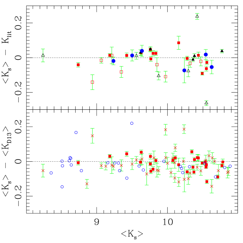
Figure 9: Our intensity-mean $\langle K_{s}\rangle$ magnitudes are compared with photometry from the literature. The error bars show our photometric uncertainties, $\sigma_{K}$, alone. (Top) Circles mark six stars with densly-populated light curves (BW stars with photometry reference #1 from Table 1) after correction to the 2MASS photometric system; squares mark 22 stars from Fernley, Skillen & Burki (1993) (reference #2) after correction to the 2MASS system; and triangles mark ten stars with unpublished photometry reported in Fernley et al. (1998) (reference #3). Filled and open symbols indicate stars observed with MDM and SMARTS, respectively. (Bottom) Our $\langle K_{s}\rangle$ magnitudes from MDM (squares) and SMARTS (crosses) are compared with mean magnitudes from Dambis et al. (2013). The circles indicate photometry taken from the literature for the BW stars (reference #1, after correction to the 2MASS system) compared with that of Dambis et al. (2013).

The stars observed by Fernley, Skillen & Burki (1993) (reference #2), after correction to $K_{s}$, scatter more widely and have a substantial offset: $\langle K_{s}\rangle-K_{F98}^{\prime}=-0.019$ with $\sigma=0.054$ mag. If the bright outlier with the large error bar (V675 Sgr) is omitted, these values become –0.013 and 0.048 mag, respectively. Part of this scatter can be attributed to errors in our observations. Subtracting in quadrature our mean $\sigma_{K}$ of 0.020 mag leaves 0.044 mag attributable to errors in the Fernley magnitudes, which we list as the magnitude uncertainty $\sigma_{F98}$ in Table 5.

The stars with unpublished photometry reported in Fernley et al. (1998) (reference #3) also scatter widely, with $\langle K_{s}\rangle-K_{F98}^{\prime}=-0.006$ and $\sigma=0.121$ mag. If we omit the two extreme outliers (TY Aps and AU Vir), these values become –0.005 and 0.052 mag, respectively, giving no evidence of a systematic offset. Subtracting our errors in quadrature indicates that 0.048 mag of the scatter can be attributed to errors in the unpublished photometry, which we list in Table 5 as $\sigma_{F98}$ for these stars.

The lower panel of Figure 9 compares our magnitudes with the those of Dambis et al. (2013). The mean difference is $\langle K_{s}\rangle-K_{D13}=-0.017$ with $\sigma=0.061$ mag for the 74 stars in common, all of which had been phased and template-fit by Dambis (2009). The four outliers (from left to right: V Ind, V675 Sgr, RV Cap, and BB Eri) have lower quality photometry from our SMARTS observations, but none is so different from the other SMARTS results as to create the offsets seen in Figure 9, and so we hypothesize that the errors for these four stars are in the Dambis (2009) photometry. If these points are rejected, the mean and standard deviation become –0.022 and 0.046 mag, respectively.

To test the hypothesis that the outliers were caused by the Dambis photometry, we matched the Dambis data with the corrected photometry for all the stars with densely-populated light curves from BW analyses, $K_{BW}^{\prime}$. Again, all stars in the comparison were phased and fit by Dambis (2009), and again there are clear outliers in the lower panel of Figure 9 (from left to right: AR Per, DX Del, and UU Vir). Each of these stars was observed as part of a different BW study, making it more likely that the discrepancies resulted from the Dambis photometry. After rejecting these three outliers, we found the remaining stars had $K_{BW}^{\prime}-K_{D13}=-0.028$ with $\sigma=0.030$ mag. The scatter is in agreement with the size of the errors indicated by Dambis (2009) and Dambis et al. (2013), while the mean is consistent with the offset we found between our observations and the Dambis data; it hints that the Dambis data may be systematically faint by $\sim$0.025 mag, though the cause of such an offset is not obvious.

We can also use the information in Figure 9 to check whether there is a systematic offset between our data taken at the SMARTS and MDM observatories. In the top panel, the observations from SMARTS tend to lie below those from MDM when compared with stars from Fernley, Skillen & Burki (1993) (reference 2) and with unpublished stars from Fernley et al. (1998) (reference 3), suggesting they may be systematically brighter. The offsets are $\langle K_{s}\rangle-K_{F98}^{\prime}=-0.041\pm 0.016$ mag and $+0.001\pm 0.012$ mag for the reference 2 data compared with data from SMARTS and MDM, respectively. They are $-0.039\pm 0.031$ and $+0.023\pm 0.011$ mag, respectively, for the reference 3 data. For the comparison shown in the bottom panel of Figure 9, the offsets are $\langle K_{s}\rangle-K_{D13}=-0.030\pm 0.007$ and $-0.013\pm 0.008$ mag for the data from SMARTS and MDM, respectively. These all suggest that our SMARTS data are systematically brighter than our MDM data. The single but very significant exception is the comparison in the top panel between our data and the highest quality data, which were obtained from previous BW studies, for which $\langle K_{s}\rangle-K_{BW}^{\prime}=-0.001\pm 0.016$ mag for the SMARTS data (no MDM data were obtained of BW stars). The weighted mean of the three offsets using the MDM data is $0.000\pm 0.006$ mag, indicating the MDM data are securely on the 2MASS system, while the weighted mean of the four offsets using the SMARTS data is $-0.028\pm 0.006$ mag, supporting the idea that these data are systematically too bright. In calculating each of these offsets, the outlier points discussed above have been removed. The choices of which stars to consider as outliers and which weighting scheme to utilize have small but meaningful effects on the size of the systematic photometric offset of the SMARTS data, which we estimate to be 0.02-0.03 mag. The origin of this offset is not known, and we recommend that independent photometric observations be acquired for some of our SMARTS stars to confirm and quantify the size of any offset.

We conclude that photometry which is based on small numbers of photometric observations – specifically, Dambis (2009), the unpublished photometry reported in Fernley et al. (1998), and to a lesser extent Fernley, Skillen & Burki (1993) – contains a small fraction of stars with random photometric errors of $\sim$0.1 mag which can not be identified a priori. This is true even of the Dambis et al. (2013) photometry that was phased with ephemerides from the literature and fit with a light curve template to obtain a star’s intensity-mean magnitude; seven of the 104 stars (7%) in the comparisons above were outliers. This is in addition to the 32 of 403 stars (8%) in Dambis et al. (2013) which had no reliable ephemeris in the literature and were expected to have random offsets of $\sim$0.1 mag. We found the outlier rates in the Fernley et al. (1998) $K$-magnitudes to be 5% for stars with reference #2 and 18% for stars with reference #3.

7.3 Photometric Means

In an effort to ameliorate the effect of any zero–point offsets, to identify and reject outliers, and to bring as much independent information as possible to bear on determining each star’s intensity-mean apparent magnitude, we developed the following scheme for combining the photometric data. First, we corrected any magnitudes from the literature to the 2MASS photometric system using the methods previously described, and compiled all the available magnitudes for each star as shown in Table 5. We computed a weighted mean for each star using the following weights, $w_{i}$, and tracked which sources were utilized using a code composed of four integers, $c_{i}$. For the stars with densely-populated BW light curves, we adopt $w_{1}=0.009^{-2}$ mag (Monson et al., 2017) and set the first digit of the code to $c_{1}=1$ for the twenty stars from Table 5 of Monson et al. (2017) including RR Lyrae itself, and the code $c_{1}=2$ for the ten BW stars not in Monson et al. (2017) which we transformed to the 2MASS system ourselves (the prime symbol in Table 5 indicates the transformation).

For the stars with our $\langle K_{s}\rangle$ values in Table 5 we adopt $w_{2}=\sigma_{K}^{-2}$ and set the second digit $c_{2}$ to “1” if the star was observed with SMARTS or “2” if it was observed using MDM. Code $c_{2}=3$ indicates that both observatories were used to observe YZ Cap and we hereafter use the weighted mean of $\langle K_{s}\rangle=10.355\pm 0.011$ mag for this star; while $c_{2}=4$ indicates the direct 2MASS observation of NSV 660. We also increased the $\langle K_{s}\rangle$ value for each star observed with SMARTS by 0.028 mag to account for the offset estimated above.

The stars in the compilation of Fernley et al. (1998), shown in Table 5 under the heading $K^{\prime}_{F98}$, are given $w_{3}=0.044^{-2}$ and $c_{3}=2$ in the third digit if it was from Fernley, Skillen & Burki (1993) (60 stars, reference #2 in Table 1), or $w_{3}=0.048^{-2}$ and $c_{3}=3$ if the data was unpublished (20 stars, reference #3). Finally, each of the stars in the compilation (except NSV 660) has a magnitude and uncertainty, $\sigma_{D13}$, from Dambis et al. (2013), which we weight with $w_{4}=\sigma_{D13}^{-2}$ mag and identify with $c_{4}=1$ in the fourth digit. Any star for which data was not available will have a value of zero in the corresponding digit of the code. For example, a star having a code of “1021” indicates the star has photometry from a high density BW source, no observation from Table 4, and had photometric values in Fernley, Skillen & Burki (1993) and Dambis et al. (2013). The combined digits of this code for each star are listed in Table 5 under the column labeled “Code_K.”

So that we could detect and reject outlier photometry for a given star, we retained only stars with two or more photometric values and computed the weighted mean and the difference of each magnitude from that mean. Data from any stars with differences more than $\pm 0.1$ mag from the weighted mean were inspected visually and if one source was clearly discrepant, it was rejected and identified with a “9” in the digit of the code corresponding to that photometric source (four stars). For seven stars with only two observations from lower-quality sources, it was difficult to distinguish outliers, and we retained the potentially discrepant photometry. Two other stars are noteworthy: V675 Sgr and RV Cap both had three measures of lower quality, and for both stars, our $\langle K_{s}\rangle$ value was bracketed by discrepant values ($|\Delta K|>0.1$ mag) from Fernley et al. (1998) and Dambis et al. (2013); since no outlier could be identified, we retained all three values when computing the weighted mean magnitude for each star. Of the 13 stars with photometric deviations larger than 0.1 mag, only RV Cap is known to exhibit the Blazhko effect, so in general these cyclic variations in amplitude can not be responsible for the outlier behavior seen in Figure 9.

For each of the remaining 146 stars, the weighted mean magnitude $\bar{\langle K\rangle}$ and its error $\sigma_{\bar{K}}$ are shown in Table 5. In the column labeled “Flag” we identify stars whose data scatter more broadly than suggested by the weighted error; these stars are strong candidates for attention in future photometric programs. Overall, our weighting scheme places high weight on the BW and MDM photometry, while weighting SMARTS photometry and that from the other sources at similar, lower levels.

7.4 Reddening Means

We used an analogous scheme for weighting and identifying the contributions of the three interstellar reddening values listed in Table 1. We used weights $w_{i}=\sigma_{i}^{-2}$, where $\sigma_{2}=0.03$ mag for the Blanco (1992) reddening $E(B-V)_{B92}$, and $\sigma_{3}=0.03$ mag for the Fernley et al. (1998) reddening $E(B-V)_{F98}$, as discussed in Sec. 2. For the dust-based reddening estimate, we adopted the uncertainty estimate from Schlegel, Finkbeiner & Davis (1998) of $\sigma_{1}=0.16~{}E(B-V)_{SD11}$, but set a minimum value of 0.01 mag so it would not unduly dominate the weighting when the reddening was small. We did not include these reddenings in the weighted mean when $E(B-V)_{SD11}>0.20$ mag, because they are systematically overestimated as shown in Sec. 2, and flagged them with $a_{1}=9$ in the first digit of a three-integer identification code. Otherwise, $a_{i}=1$ indicates that a value was used in the weighted mean, while 0 indicates the value was not available. Using $A_{K}=0.36~{}E(B-V)$ from Cardelli, Clayton, & Mathis (1989), we converted the weighted mean reddening and its error into interstellar absorption, $A_{K}$, and its error $\sigma_{A}$, which we list in Table 5 for each star along with the integer code labeled “Code_A.”

We note that Dambis et al. (2013) provided an independent set of extinction values, $A_{V}$, in their compilation, obtained from an iterative solution to the 3D dust distribution model of Drimmel, Cabrera-Lavers, & López-Corredoira (2003). We again used $A_{K}=0.36~{}E(B-V)$ along with $A_{V}=3.1~{}E(B-V)$ from Cardelli, Clayton, & Mathis (1989) to convert these optical extinction values to infrared, and compare them with our own. For the 145 stars in common, the mean difference $A_{K}-A_{K}(D13)=-0.0002$ mag with a standard deviation $\sigma=0.007$ mag, indicating outstanding agreement between our data sets.

Table 7: Final Data for Absolute Magnitude Solutions

Star	Type	$m_{K,o}$	$\sigma_{K,o}$	[Fe/H]	$\sigma_{\mathrm{[Fe/H]}}$	$\log{P_{f}}$	Gaia ID	$\varpi$	$\sigma_{\varpi}$	$M_{K_{s}}$	$\sigma_{M_{K}}$
SW And	ab	8.494	0.009	–0.24	0.09	–0.354304	2857456207478683776	1.7797	0.1636	–0.254	0.210
XX And	ab	9.429	0.027	–1.94	0.16	–0.141017	370067649378653440	0.6950	0.0463	–1.361	0.152
AT And	ab	9.026	0.028	–1.18	0.13	–0.209776	1925406252226143104	2.1779	0.2715	+0.716	0.291
DM And	ab	10.515	0.009	–2.32	0.15	–0.200391	1912453760434108928	0.6000	0.0617	–0.594	0.236
$\cdots$	$\cdots$	$\cdots$	$\cdots$	$\cdots$	$\cdots$	$\cdots$	$\cdots$	$\cdots$	$\cdots$	$\cdots$	$\cdots$
AV Vir	ab	10.547	0.013	–1.25	0.16	–0.182496	3731723090075245696	0.5297	0.0470	–0.833	0.202
BN Vul	ab	8.557	0.027	–1.61	0.22	–0.226122	2022835523801236864	1.4014	0.0301	–0.710	0.054
NSV 660	ab	13.976	0.020	–1.31	0.10	–0.196141	2507784713545431424	0.0567	0.0444	–2.228	3.318

Note. — (This table is available in its entirety in machine-readable form.)

8 Gaia Parallaxes and the RR Lyrae Luminosity Calibration

In Table 7, we compile the data needed to perform period-luminosity-metallicity (PLZ) fits on our RRL sample. The column labeled $m_{K,o}$ contains the mean apparent magnitude $\bar{\langle K\rangle}$ from Table 5 after correction for interstellar absorption $A_{K}$, and the column labeled $\sigma_{K,o}$ lists its uncertainty computed by adding the uncertainties from those values in quadrature. The metallicity [Fe/H] was taken from Table 1, using the value from Fernley et al. (1998) if one is available, and using the value from Layden (1994) if it was not. The weights $\sigma_{\mathrm{[Fe/H]}}$ are as described in Sec. 2.1. The logarithm of the adopted period from Table 4 is presented as $\log{P_{f}}$, where any star with a pulsation type “c” has been fundametalized by adding 0.127 to the logarithm of its period.

We searched the Gaia Data Release 2 (DR2) catalog (Gaia Collaboration et al., 2016b, 2018a) using a search cone with 2-4 arcsec radius around the 2MASS coordinates listed in Table 1. In every case we obtained only one match, and we checked this star’s parallax, proper motion, and magnitude with values from the literature to ensure that we had correclty identified the RRL. Each star’s unique Gaia identifier number is listed in Table 7 along with its parallax value $\varpi$ and its uncertainty $\sigma_{\varpi}$ in units of milli-arcseconds (mas). The parallax for the star RR Lyrae is negative as its mean $G$ magnitude was determined incorrectly in DR2 (Muraveva et al., 2018), and so we do not use this star in our analysis.

The DR2 catalog is known to contain spurious parallaxes which formally have small parallax uncertainties. Spurious parallaxes typically have a large astrometric $\chi^{2}$ and the Gaia team recommend that one calculates the Unit Weight Error (Lindegren et al., 2018) to find spurious astrometric solutions

$$\mathrm{UWE}=\sqrt{\chi^{2}/(N-1)}$$

where $\chi^{2}=$ astrometric_chi2_al and
$N=$ astrometric_n_good_obs_al are available in the DR2 catalog. Large values of UWE indicate a bad astrometric solution. Lindegren et al. (2018) further recommend that the RUWE, which depends on the color and magnitude is a better way to determine if an astrometric solution is spurious. However, since RRL have variable colors and magnitudes, it is not possible to calculate RUWE from the data provided in DR2, and so we elect to use the UWE to search for spurious parallaxes. The UWE was calculated for each of our stars, and two stars were found to have large UWE values $>2.5$: VV Peg (UWE $=6.9$) and AT And (UWE = $12.8$). We do not use these stars in any further analysis, leaving our RRL sample with 143 stars.

The uncertainties in the DR2 parallaxes are known to be underestimated by $\sim$30$\%$ (Gaia Collaboration et al., 2018c, b) for the brighter sources. Lindegren et al. (2018) have presented a tentative calibration of the true, external error in the Gaia DR2 parallaxes, $\sigma_{ext}=\sqrt{1.08^{2}\sigma_{i}^{2}+\sigma_{s}^{2}}$, where $\sigma_{i}$ is the internal parallax error reported for each star in DR2, and $\sigma_{s}=0.021\,$mas for bright ($G\lesssim 13$) stars and $\sigma_{s}=0.043\,$mas for faint ($G>13$) stars. We have applied this correction to the reported parallax uncertainties in all of our analysis, though we list the DR2 values as provided in Table 7. Using these increased uncertainties, the median value of $\varpi/\sigma_{\varpi}=18.2$ for stars which we use in our analysis, with only two stars having $\varpi/\sigma_{\varpi}<5.0$, indicating the high quality of the parallaxes now available.

For each star in Table 7 we calculated the absolute magnitude (along with its uncertainty, $\sigma_{M_{K}}$) in the 2MASS $K_{s}$ photometric system using

$$M_{K_{s}}=m_{K,o}+5~{}\rm{log}_{10}(\varpi)-10.$$ (3)

These values are listed in Table 7 and plotted against the logarithm of the stars’ pulsation periods in Figure 10 for all 143 RRL with reliable DR2 parallaxes in our sample. We note that Gaia Collaboration et al. (2018c) strongly recommend against using the parallax to directly infer the distance (as in the above equation) when deriving astrophysical parameters. Given that our sample selection was not based upon DR2 data, and the generally high quality of the DR2 parallaxes in our sample, much of the reasoning presented by Gaia Collaboration et al. (2018c) does not apply to our case. Figure 10 is informative, though we don’t use it our subsequent analysis.

Figure 10: The parallax-based absolute magnitude $M_{K_{s}}$ from Table 7 is plotted against the logarithm of the period for 143 RRL stars. The RRc stars had their periods fundamentalized by adding 0.127 to $\log P$ in the right panel. The RRab stars are divided into two metallicity groups as indicated in the legend, corresponding to the disk and halo kinematic populations (see Sec. 2.4); there are no metal-rich RRc stars in this sample. Three stars that are outliers from our PLZ fit (see Sec. 8.3) are marked in orange. A DR2 parallax zero-point error of $-0.036\,$mas was assumed when determining $M_{K_{s}}$.

The c-type RRL form a grouping on the left with shorter periods. A trend with log $P$ is apparent for both RRab and RRc stars. We note that if the period of the RRc stars is “fundamentalized” by adding 0.127 to $\log P$, then the RRc stars appear well mixed with the RRab stars. There is a clear tendency for the metal-rich RRab stars to be fainter than the metal-poor RRab stars, indicating that a PLZ relation exists in the data.

8.1 PLZ Fitting Procedure

To explore the PLZ relation for RRLyr stars in the $K_{s}$ band we use the astrometric based luminosity (ABL) prescription of Arenou & Luri (1999). The ABL approach avoids biases caused by converting to magnitudes, allows the use of low-quality parallax measurements (including NSV 660) and has been shown to yield similar results to a Baysian analysis when examining PL and PLZ relations (Gaia Collaboration et al., 2016b). Because we use the data for all the stars in our sample and do not truncate the sample at an “observed” relative error, $\varpi/\sigma_{\varpi}$, we do not introduce a systematic error in absolute magnitude of the type discussed by Lutz & Kelker (1973), a point made by Arenou & Luri (1999) along with some other noteworthy interpretations. Arenou & Luri (1999) defined the ABL to be

$$a_{K}=10^{0.2M_{K}}=\varpi 10^{0.2m_{K,o}-2}$$ (4)

where $M_{K}$ is the $K_{s}$ absolute magnitude, $\varpi$ is the parallax in mas and $m_{K,o}$ is the extinction corrected apparent magnitude. The PLZ relation may be written as

$$M_{K}=\beta_{1}+\beta_{2}(\log P+0.27)+\beta_{3}([\mathrm{Fe/H}]+1.3)\,,\\$$ (5)

where one determines the coefficients $\beta$ from a fit to the data. The addition of 0.28 to $\log P$ and 1.3 to [Fe/H] minimizes the uncertainty in the zero-point found by the fit, as the average value of $\log P=-0.27$ and the average $[\mathrm{Fe/H}]=-1.3$ in this dataset. In the ABL approach, the following equation is used to determine the PLZ relation

$$\varpi 10^{0.2m_{K,o}-2}=10^{0.2[\beta_{1}+\beta_{2}(\log P+0.27)+\beta_{3}([\mathrm{Fe/H}]+1.3)]}\;.$$ (6)

In analyzing the global luminosity properties of DR2 stars, one must take into account that there exists a global zero-point parallax error in DR2 (Gaia Collaboration et al., 2018a, b, c). An analysis of quasars indicates the zero-point error is $-0.029\,$mas for fainter objects (Gaia Collaboration et al., 2018a), and there are indications from the quasar sample that the zero-point error increases ($\sim$0.05 mas) at brighter magnitudes (Gaia Collaboration et al., 2018a). All of the quasars are fainter than our RR Lyr dataset. External comparisons to relatively bright stars with VLBI or HST FGS parallaxes indicate a zero-point error of $-0.07\pm 0.03\,$mas and $\-0.01\pm 0.02\,$mas respectively (Gaia Collaboration et al., 2018b). These comparisons, along with other analysis led the Gaia collaboration to conclude that the global zero-point is less than $0.1\,$mas. This has been verified by Stassun & Torres (2018), who compare Gaia DR2 distances to distances determined to relatively bright eclipsing binaries and find a DR2 zero-point error of $-0.08\pm 0.03\,$mas. The parallax zero-point error varies spatially (Gaia Collaboration et al., 2018a, b), but since our RR Lyr stars are randomly distributed across the sky, it is only the global zero-point error which is of importance to our PLZ analysis. Allowing for a global zero-point error requires the use of an implicit fitting function,

$$f \equiv 10^{0.2[\beta_{1}+\beta_{2}(\log P+0.27)+\beta_{3}([\mathrm{Fe/H}]+1.3)]}$$ (7)

$$- (\varpi+\beta_{4})10^{0.2m_{K,o}-2}=0$$

where $\beta_{4}=\pi_{zp}$ is determined as part of the fitting process.

In performing fits to data, one weights the fit by the uncertainty in the data. Many of the stars in our dataset have very well determined parallaxes and mean magnitudes, with very small formal uncertainties. However, the recent paper by Braga et al. (2018) which presents $JHK$ photometry of RRL in $\omega\,$Centauri suggests that there is an intrinsic dispersion in the PLZ relation. Braga et al. (2018) fit the PLZ relation for a large number of stars spanning $-2.3<[\mathrm{Fe/H}]<-1.3$. Depending on which metallicities are employed (Rey et al., 2000; Sollima et al., 2006; Braga et al., 2016), standard deviations of the RRL around the best-fit PLZ relations are 0.045, 0.029, and 0.039 mag, respectively for their “global” solutions where RRab and fundamentalized RRc are in the same fit. The residual magnitude distributions in their Figures 19, 20 and 21 appear to be roughly Gaussian. These standard deviations are larger than the photometric uncertainties in their data as the the median of their $K_{s}$ uncertainties is 0.008 mag for 198 RRL in their Table 2. Taking this at face value and subtracting it in quadrature from the above standard deviations gives an estimate of the intrinsic dispersion in $M_{K}$ in the PLZ relation of approximately 0.03 to 0.04 mag. To take into account the intrinsic dispersion in the PLZ relation, when performing the fits, the uncertainty in the $K_{s}$ magnitude is found by adding the photometric uncertainty in quadrature with an intrinsic dispersion of $\sigma_{M_{K},\,\mathrm{intrinsic}}=0.04\,$mag.

8.2 Monte Carlo Tests

The implicit nonlinear weighted orthogonal distance fitting was performed using ODRPACK95 (Zwolak et al., 2007), which is an updated version of ODRPACK (Boggs et al., 1989). This fitting routine takes into account the uncertainties in the photometry, extinction corrections, parallaxes, [Fe/H] values and periods. To test the reliability of the fitting procedure and the reported uncertainties, we conducted a Monte Carlo simulation with synthetic data. In this simulation, we randomly created data sets (with $N=143$ stars) whose distribution in apparent $K_{s}$ magnitude, period and [Fe/H], along with their associated uncertainties, were all drawn randomly from the observed distributions. A PLZ relation (including an intrinsic $M_{K}$ dispersion of 0.04 mag) was specified and used to determine a ‘true’ parallax for the star. This true parallax was then used to create a simulated parallax by randomly selecting a value from a Gaussian distribution whose mean is the ‘true’ parallax, and whose standard deviation was drawn randomly from the distribution of standard deviations in the actual data. A specified zero-point error was then added to each simulated parallax. This results in a simulated dataset whose properties resemble the actual dataset. The simulation was performed 1000 times for a number of different choices of the PLZ relation and parallax zero-point error. The simulated data was then used by our fitting program to calculate the PLZ relation.

These initial tests indicated that ODRPACK95 was reliably determining the zero-points in our fitting function ($\beta_{1}$ and $\beta_{4}$ in equation 7), but did not determine the slopes ($\beta_{2}$ and $\beta_{3}$ in equation 7) reliably. As a result, we adopted a two-step procedure for our fits. After performing the implicit fit with ODRPACK95 and determining the DR2 global parallax offset, we then performed an explicit nonlinear fit (equation 6) using gnuplot. The Monte Carlo tests indicate that this two-step fitting procedure does an excellent job of recovering the input PLZ relation and the parallax zero-point, including estimating the uncertainties in the coefficients. The latter point is demonstrated by the fact that the standard deviation of the Monte Carlo results ($\sigma_{\mathrm{MC}}$) is very similar to the average (over all the Monte Carlo simulations) of the errors reported by the fitting procedure ($\langle\mathrm{MC~{}Err}\rangle$). The results of our Monte Carlo tests for our two-step fitting procedure are summarized in Table 8. The first two Monte Carlo tests shown in Table 8 use identical input parameters, and the differences in the output reflect the statistical uncertainty in our Monte Carlo.

In performing the nonlinear fitting with the actual data, the goodness of fit was determined by an analysis of the normalized fit residuals ($R_{i}\equiv f_{i}/\sigma_{f_{i}}$, where $i$ represents the $i^{\mathrm{th}}$ star in the observed dataset), as $\chi^{2}$ analysis is not appropriate for a nonlinear fit (Andrae et al., 2010). The fit residuals should follow a Gaussian distribution, with a mean $\mu=0$ and variance $\sigma^{2}=1$.

Since our fitting function is a fairly complicated nonlinear function, uncertainty in its value for a given star was determined through a Monte Carlo simulation, where specific values for each of the variables ($\beta_{1};\beta_{2};\beta_{3};\beta_{4};\log P;[\mathrm{Fe/H]};m_{K,o},\varpi$) was randomly drawn from a Gaussian distribution whose mean and standard deviation are given by their tabulated values for the observed values or returned by the two-step fitting procedure for the fitted parameters. This was repeated 1000 times for each star, and the resulting distribution of $f_{i}$ was used to determine the uncertainty, $\sigma_{f_{i}}$.

Table 8: Monte Carlo Test of ABL Fitting Procedure

Parameter	Input	MCmean	Difference	$\sigma_{\mathrm{MC}}$	$\langle\mathrm{MC~{}Err}\rangle$
PLZ zero-point:	$-0.450$	$-0.447$	$-0.003$	$0.026$	$0.028$
PLZ Period slope:	$-2.700$	$-2.697$	$-0.003$	$0.148$	$0.146$
PLZ [Fe/H] slope:	$0.300$	$0.300$	$0.000$	$0.022$	$0.022$
Parallax zero-point:	$-0.040$	$-0.040$	$0.000$	$0.011$	$0.011$
PLZ zero-point:	$-0.450$	$-0.446$	$-0.004$	$0.027$	$0.028$
PLZ Period slope:	$-2.700$	$-2.696$	$-0.004$	$0.153$	$0.146$
PLZ [Fe/H] slope:	$0.300$	$0.300$	$0.000$	$0.023$	$0.022$
Parallax zero-point:	$-0.040$	$-0.041$	$0.001$	$0.011$	$0.011$
PLZ zero-point:	$-0.450$	$-0.447$	$-0.003$	$0.027$	$0.028$
PLZ Period slope:	$-2.700$	$-2.692$	$-0.008$	$0.155$	$0.144$
PLZ [Fe/H] slope:	$0.300$	$0.300$	$0.000$	$0.023$	$0.022$
Parallax zero-point:	$-0.080$	$-0.080$	$0.000$	$0.011$	$0.011$
PLZ zero-point:	$-0.450$	$-0.449$	$-0.001$	$0.024$	$0.024$
PLZ Period slope:	$-2.700$	$-2.694$	$-0.006$	$0.154$	$0.145$
PLZ [Fe/H] slope:	$0.100$	$0.101$	$-0.001$	$0.023$	$0.022$
Parallax zero-point:	$-0.080$	$-0.080$	$0.000$	$0.010$	$0.010$
PLZ zero-point:	$-0.450$	$-0.445$	$-0.005$	$0.025$	$0.028$
PLZ Period slope:	$-2.400$	$-2.395$	$-0.005$	$0.153$	$0.146$
PLZ [Fe/H] slope:	$0.300$	$0.300$	$0.000$	$0.022$	$0.022$
Parallax zero-point:	$-0.040$	$-0.041$	$0.001$	$0.010$	$0.011$
PLZ zero-point:	$-0.550$	$-0.547$	$-0.003$	$0.025$	$0.027$
PLZ Period slope:	$-2.600$	$-2.589$	$-0.011$	$0.152$	$0.153$
PLZ [Fe/H] slope:	$0.200$	$0.202$	$-0.002$	$0.024$	$0.023$
Parallax zero-point:	$-0.030$	$-0.030$	$0.000$	$0.010$	$0.011$
PLZ zero-point:	$-0.550$	$-0.548$	$-0.002$	$0.025$	$0.027$
PLZ Period slope:	$-2.600$	$-2.598$	$-0.002$	$0.160$	$0.155$
PLZ [Fe/H] slope:	$0.200$	$0.200$	$0.000$	$0.024$	$0.023$
Parallax zero-point:	$-0.010$	$-0.010$	$0.000$	$0.010$	$0.011$
PLZ zero-point:	$-0.450$	$-0.448$	$-0.002$	$0.023$	$0.024$
PLZ Period slope:	$-3.000$	$-2.997$	$-0.003$	$0.157$	$0.146$
PLZ [Fe/H] slope:	$0.100$	$0.100$	$0.000$	$0.023$	$0.022$
Parallax zero-point:	$-0.030$	$-0.030$	$0.000$	$0.010$	$0.010$
PLZ zero-point:	$-0.450$	$-0.450$	$0.000$	$0.024$	$0.024$
PLZ Period slope:	$-2.800$	$-2.800$	$0.000$	$0.151$	$0.147$
PLZ [Fe/H] slope:	$0.050$	$0.050$	$0.000$	$0.022$	$0.022$
Parallax zero-point:	$-0.030$	$-0.029$	$-0.001$	$0.010$	$0.010$
PLZ zero-point:	$-0.500$	$-0.496$	$-0.004$	$0.026$	$0.026$
PLZ Period slope:	$-2.300$	$-2.292$	$-0.008$	$0.159$	$0.150$
PLZ [Fe/H] slope:	$0.180$	$0.180$	$0.000$	$0.023$	$0.023$
Parallax zero-point:	$-0.050$	$-0.051$	$0.001$	$0.011$	$0.011$

8.3 PLZ of the Observed RRL

In order to evaluate how different [Fe/H] scales and weighting schemes may impact our fitted PLZ relations, we used four different datasets in the analysis of our observed RRL, each with a slightly different way of determining [Fe/H]:

F0

The [Fe/H] estimates from Fernley et al. (1998) and Layden (1994) were adopted without correction, and a uniform uncertainty of $\pm 0.20\,$dex was assumed for each [Fe/H] value.

F1

No correction was applied to the Fernley et al. (1998) and Layden (1994) [Fe/H] estimates, and the weights $\sigma_{\mathrm{[Fe/H]}}$ were adopted from Table 7.

F2

The Fernley et al. (1998) [Fe/H] values were shifted by $-0.06\,$dex to put them onto the Layden (1994) [Fe/H] scale, and the weights were adopted from Table 7.

F3

The Layden (1994) [Fe/H] values were shifted by $+0.06\,$dex to put them onto the Fernley et al. (1998) scale, and the weights were adopted from Table 7.

Table 9: P-L-Z Fits of Observed RRL

	PLZ				$\chi^{2}$
Dataset	Zero-point	$\log P$ slope	[Fe/H] slope	$\pi_{zp}$	residuals
F0	$-0.427\pm 0.035$	$-2.87\pm 0.19$	$0.122\pm 0.024$	$-0.036\pm 0.015$	1.15
F0 no outliers	$-0.408\pm 0.032$	$-2.82\pm 0.17$	$0.122\pm 0.022$	$-0.040\pm 0.013$	1.07
F1	$-0.424\pm 0.033$	$-2.86\pm 0.19$	$0.122\pm 0.024$	$-0.037\pm 0.014$	1.16
F1 no outliers	$-0.405\pm 0.031$	$-2.81\pm 0.17$	$0.122\pm 0.022$	$-0.042\pm 0.013$	1.08
F2	$-0.414\pm 0.033$	$-2.86\pm 0.19$	$0.123\pm 0.024$	$-0.038\pm 0.014$	1.16
F2 no outliers	$-0.394\pm 0.031$	$-2.81\pm 0.17$	$0.123\pm 0.022$	$-0.043\pm 0.013$	1.08
F3	$-0.423\pm 0.033$	$-2.86\pm 0.19$	$0.123\pm 0.024$	$-0.038\pm 0.014$	1.16
F3 no outliers	$-0.403\pm 0.031$	$-2.81\pm 0.17$	$0.123\pm 0.022$	$-0.043\pm 0.013$	1.08

Results of fitting the PLZ relation to the different datasets are given in Table 9. The last column in the table gives the variance of the residuals from the fit, which would be 1.0 for a good fit. There are three outlier with residuals $\geq 3\,\sigma$ in the fit: RR Gem, an RRab star with $[\mathrm{Fe/H}=-0.29$, $\log P=-0.40$, $R=3.6$; TT Lyn, an RRab star with $[\mathrm{Fe/H}=-1.56$, $\log P=-0.22$, $R=3.4$; and RU Psc, an RRc star with $[\mathrm{Fe/H}=-1.75$, $\log P=-0.41$, $R=3.0$. There is no indication from the photometry or the DR2 astrometric $\chi^{2}$ that the parallaxes of these three stars are in error. However, since in a sample of 143 stars, one does not expect any $\geq 3\,\sigma$ outliers, we also performed the fit with these three stars removed. The goodness of fit is improved when these three stars are removed. Removing the outliers does not lead to a significant change in the slopes of the fitted PLZ relation, and has a modest ($0.02\,$mag) effect on the zero-point.

Regardless of exactly how we determine the [Fe/H] values of the stars, the fits are all quite similar, and agree with each other within their uncertainties. Given our preference for the F1 metallicity scale, we determine the following PLZ relation

$$M_{K_{s}} = (-2.8\pm 0.2)(\log P+0.27)$$

$$+ (0.12\pm 0.02)([\mathrm{Fe/H}]+1.3)-(0.41\pm 0.03)$$

with $\pi_{zp}=-0.042\pm 0.013\,$mas.

The quality of the fit may be visually assessed using a quantile-quantile plot (see Figure 11) to examine the normalized residuals. It has been shown that the quantile-quantile plot is superior to many other techniques (e.g.  Anderson-Darling, Shapiro-Wilk or Cramér-von Mises tests) in determining if a distribution is Gaussian (Loy et al., 2016). In the quantile-quantile plot, the quantiles of the observed distribution are plotted as a function of the quantiles of the theoretical distribution. The slope of the quantile-quantile plot is the standard deviation of the observed distribution, and the intercept is the mean of the observed distribution. Figure 11 shows the residuals of the F1 fit which does not include the three outliers (RR Gem, TT Lyn and RU Psc). The standard deviation of the residuals (slope in Fig. 11) is a bit larger than one, which suggests that there is some additional dispersion in the data which has not been captured by the fit.

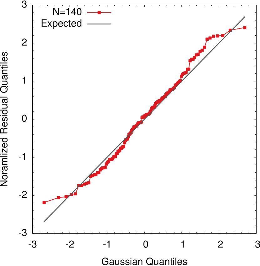
Figure 11: A quantile-quantile plot of the normalized residuals for the fit to the stars in the F1 [Fe/H] scale, with outliers removed. A good fit will result in Gaussian residuals, with a standard deviation of $\sigma=1$ and a mean $\mu=0$, which is shown by the straight line.

Figure 12 plots projections of the PLZ relation and residuals in the $\log P$-$M_{K_{s}}$ and [Fe/H]-$M_{K_{s}}$ planes. The three outliers are shown in orange, and were not included in the fit. There are no obvious residual trends.

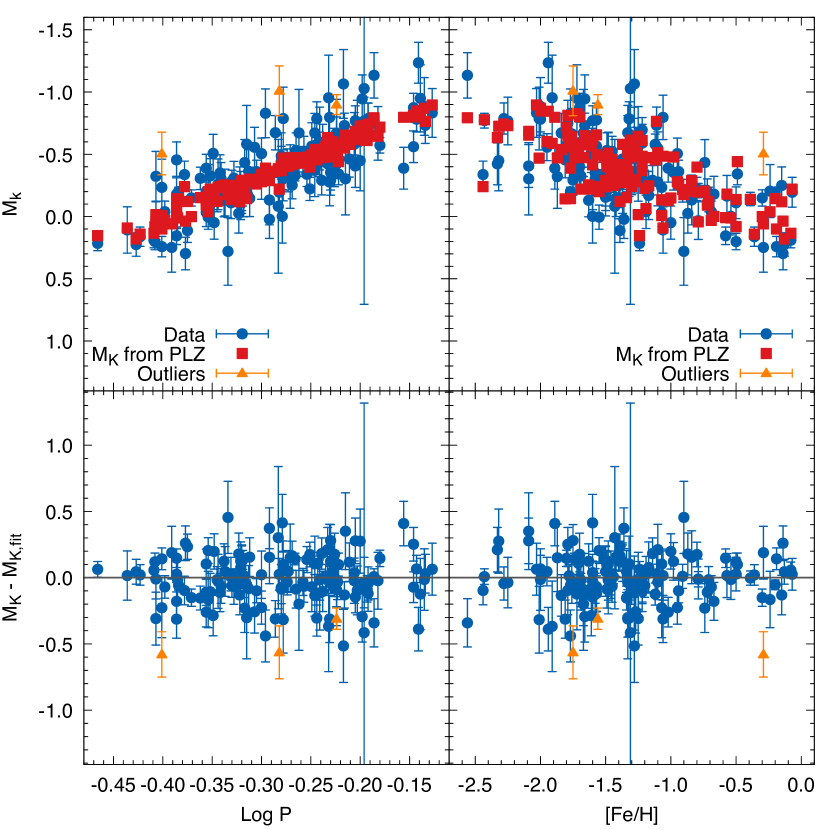
Figure 12: The PLZ relation projected onto the PL (left) and PZ planes (right). The upper panels show the $M_{K}$ values derived by assuming the distance is simply related to the parallax (Equation 3, including the DR2 zero-point error found by the fit) along with the $M_{K}$ values derived from the PLZ fit from Equation 8.3, and the lower panel shows the absolute magnitude residuals.

Our PLZ relation in $K_{s}$ may be compared to other determinations in the literature. Using data for 396 field RRL with DR2 parallaxes along with the single-epoch $K_{s}$ apparent magnitudes and reddening values from Dambis et al. (2013), Muraveva et al. (2018) found

$$M_{K_{s}} = (-2.44\pm 0.35)\log P$$

$$+ (0.18\pm 0.07)[\mathrm{Fe/H}]-(0.81\pm 0.18)$$

and a DR2 global parallax error of $\pi_{zp}=-0.051\pm 0.01$ mas. At $[\mathrm{Fe/H}]=-1.3$ and $\log P=-0.27$, their relation implies $M_{K_{s}}=-0.40\pm 0.18\,$mag which agrees very well with the zero-point of our PLZ relation. Our period slope is somewhat steeper (by $0.89\,\sigma$) than the Muraveva et al. (2018) period slope, while our [Fe/H] slope differs by $0.82\,\sigma$. The uncertainties given by Muraveva et al. (2018) are all larger than our uncertainties, except for the uncertainty in $\pi_{zp}$, which is slightly better constrained in their analysis. Muraveva et al. (2018) performed a Bayesian analysis, and it is unclear if the differences between our results and Muraveva et al. (2018) are due to the different datasets employed, or the different analysis techniques. Our approach of “centering” the period and metallicity distributions by applying shifts of 0.27 and 1.3 respectively, minimizes the formal uncertainty in the fitted zero point, $\beta_{1}$. It is worth noting that our set of RRL is a subset, comprising most of the brighter, best-measured stars in the samples of Muraveva et al. (2018) and Dambis et al. (2013), but using different apparent magnitudes, reddenings, and [Fe/H] values.

Our [Fe/H] slope agrees with that found by Braga et al. (2018), who determined slopes ranging from $0.062$ to $0.152$ depending on which set of [Fe/H] estimates they used in their fits. Braga et al. (2018) found a period slope of $-2.3\pm 0.1$, which is $2.2\,\sigma$ shallower than our slope. Our period slope is in agreement with Muraveva et al. (2015), who analyzed 70 RRL in the LMC and found a period slope of $-2.73\pm 0.25$, while their [Fe/H] slope of $0.03\pm 0.07$ is $1.2\,\sigma$ shallower than our [Fe/H] slope. From theoretical models, Marconi et al. (2015) predict $M_{K}=-2.25\log P+0.18[Fe/H]-0.82$ while Catelan et al. (2004) predict $M_{K}=-2.35\log P+0.175\log Z-0.60$. In both cases, our period slope is steeper and our [Fe/H] slope is shallower than the theoretical predications. The differences are $\sim 2\sigma$ for the period slope and $\sim 3\sigma$ for the [Fe/H] slope. It will be interesting to see if the slopes we find with the DR2 dataset are confirmed using the forthcoming Gaia data releases; if they are confirmed, this would indicate a possible problem with the theoretical models.

We explored subdividing our sample at $[\mathrm{Fe/H}]\approx-0.90\,$dex into disk and halo groups (see Sec. 2.4) to test whether these kinematically distinct populations – which likely have different ages and chemical evolution histories – have distinct luminosities. However, the number of disk stars in our current sample was too small to obtain an acceptable fit. Similar attempts to subdivide the halo sample into groups based on their period-shift behaviors, following the methods of Lee & Carney (1999), were also compromised by the small number of stars available which led to poor fits with large uncertainties and non-Gaussian residuals. We were thus unable to test whether these field RRL, analogous to the Oosterhoff I and II groups found in Galactic globular clusters, have distinct luminosities. As the Gaia mission continues and high-quality parallaxes become available for larger samples of stars, it will be interesting to see how the PLZ results for the disk, Oosterhoff I and Oosterhoff II samples develop.

9 Summary

We obtained over one thousand photometric measurements in the $K_{s}$ bandpass for 74 field RRL spread across the sky. Our data are calibrated directly to the 2MASS photometric system using on-image comparison stars. The RRL were selected to be relatively bright, with low interstellar reddenings, and to span a wide range of metallicity. We favored stars with poor or no multi-epoch $K$-band photometry in the literature, and tended to avoid stars known to exhibit the Blazhko effect.

We fit the phased observations for each star with a set of templates (Jones et al., 1996) to obtain the star’s intensity-mean magnitude in $K_{s}$. We checked the phase shift produced by the fit by comparing with the phasing of (near) contemporaneous optical photometry. In cases where there were too few observations to constrain the fit (eight of our 74 RRL stars), we used optical photometry to determine the phase and amplitude of the appropriate template and fitted to find the intensity-mean magnitude. We provide a careful analysis of the resulting photometric uncertainties; the typical uncertainty in the intensity-mean magnitude is 0.029 mag for stars observed with SMARTS, and 0.013 mag for stars observed from MDM.

We compared our data with multi-epoch photometry in the literature after correcting it to the $K_{s}$ system. We found excellent agreement between our data and the high quality light curves obtained for Baade-Wesselink analyses, and generally good agreement, though with larger scatter, was found with the more sparse light curves of Fernley et al. (1998) and the phased, single-epoch photometry of Dambis et al. (2013). There is some evidence that our photometry taken with SMARTS is systematically too bright by 0.02-0.03 mag, while that of Dambis et al. (2013) may be too faint by a similar amount; we encourage independent confirmation of this. We found that $\sim$10% of the stars from sources utilizing few observations (Fernley et al., 1998; Dambis et al., 2013) are outliers by $\sim$0.1 mag, perhaps because the ephemerides used to phase these stars’ photometry were outdated. An additional 8% of the RRL in Dambis et al. (2013), generally ones fainter than those in our sample, are expected to suffer larger scatter because optical ephemerides were not available to allow their single-epoch 2MASS photometry to be phased and fit with a template. Together, these outliers may be a fundamental source of error in forthcoming studies of $M_{K}$(RR) relations which use new data released by Gaia. We combined our photometry with these other sources using outlier rejection to provide a catalog of 146 RRL with reliable $K_{s}$ photometry.

We obtained estimates of the interstellar reddening toward each RRL from up to three independent sources and combined them to obtain a value for the interstellar extinction of each star. These are in excellent agreement with the independent values of Dambis et al. (2013).

We used the Gaia DR2 parallaxes for these stars to calculate their absolute magnitudes, and analyzed them using the astrometric based luminosity prescription of Arenou & Luri (1999), our implementation of which determines the global zero-point parallax error in DR2 for our sample. We obtained a RRL PLZ relationship (see Equation 8.3) by including an intrinsic dispersion in $M_{K_{s}}$ of 0.04 mag which we estimated from the RRL in $\omega$ Centauri. We estimated the uncertainties in the PLZ coefficients using Monte Carlo simulations, and the results were in good agreement with the uncertainties reported by our implicit non-linear fitting routines, giving us confidence that the reported uncertainties in our PLZ relationship are realistic. Our PLZ relation is in reasonable agreement with other PLZ relations in the literature that used DR2 parallaxes, as well as other approaches to determining the PLZ relation. We identified three stars that were outliers from this fit: if they remain outliers when analyzed using parallaxes from future Gaia data releases, then their photometry, [Fe/H] and reddening estimates should be reexamined.

References

- Andrae et al. (2010) Andrae, R., Schulze-Hartun, T. & Melchior, P. 2010 arXiv:1012.3754
- Arenou & Luri (1999) Arenou, F. & Luri, X. 1999, in ASP Conference Series, eds. D. Egret & A. Heck, 167, 13
- Beers et al. (2000) Beers. T. M., Chiba, M., Yoshii, Y., Platais, I., Hanson, R. B., Fuchs, B., & Rossi, S. 2000, AJ, 119, 2866
- Belokurov et al. (2017) Belokurov, V., Erkal, D., Deason, A. J., Koposov, S. E., De Angeli, F., Evans, D. W., Fraternali, F., & Mackey, D. 2017, MNRAS, 466, 4711
- Blanco (1992) Blanco, V. M. 1992, AJ, 104, 734
- Boggs et al. (1989) Boggs, P. T., Byrd, R.H., Donaldson, J.R. & Schnabel, R.B. 1989, ACM Transactions on Mathematical Software, 15, 348
- Bookmeyer et al. (1977) Bookmeyer, B. B., Fitch, W. S., Lee, T. A., Wisniewski, W. Z., & Johnson, H. L. 1977, Rev. Mex. Astr. Ap., 2, 235
- Braga et al. (2016) Braga, V. F., Stetson, P. B., Bono, G., et al. 2016, AJ, 152, 170
- Braga et al. (2018) Braga, V.F., Stetson, P. B., Bono, G., et al. 2018, AJ, 155, 137
- Burstein & Heiles (1978) Burstein, D. & Heiles, C. 1978, ApJ, 225, 40
- Cacciari (2013) Cacciari, C. 2013, IAU Symposium No. 289, ed. R. de Grijs, 101
- Cacciari, Clemintini & Fernley (1992) Cacciari, C., Clemintini, G., & Fernley, J. A. 1992, ApJ, 396, 219
- Cardelli, Clayton, & Mathis (1989) Cardelli, J. A., Clayton, G. C., & Mathis, J. 1989, ApJ, 345, 245
- Carpenter (2003) Carpenter, J. 2003, www.astro.caltech.edu/~jmc/2mass/v3/transformations/, accessed 2018 May 18.
- Carretta et al. (2000) Carretta, E., Gratton, R. G., Clementini, G., & Fusi Pecci, F. 2000, ApJ, 533, 215
- Catelan et al. (2004) Catelan, M., Pritzl, B. J. & Smith, H. A. 2004, ApJS, 154, 633
- Chaboyer et al. (1996) Chaboyer, B., Demarque, P., Kernan, P., Krauss, L., & Sarajedini, A. 1996, MNRAS, 283, 683
- Chaboyer et al. (2005) Chaboyer, B., Carney, B. W., Duncan, D. K., Girard, T. M., Latham, D. W., Layden, A. C., McWilliam, A., Sarajedini, A. & Shao, M. 2005, BAAS, 37, 454
- Dambis (2009) Dambis, A. K. 2009, MNRAS, 396, 553
- Dambis et al. (2013) Dambis, A. K., Berdnikov, L. N., Kniazev, A. Y., Kravtsov, V. V., Rastorguev, A. S., Sefako, R. & Vozyakova, O. V. 2013, MNRAS, 435, 3206
- Dékány et al. (2018) Dékány, I., Hajdu, G., Grebel, E., Catelan, M., Elorrieta, F., Eyheramendy, S., Majaess, D., & Jordán, A. 2018, ApJ, 857, 54
- Drimmel, Cabrera-Lavers, & López-Corredoira (2003) Drimmel, R., Cabrera-Lavers, A., & López-Corredoira, M. 2003, A&A, 409, 205
- Feast et al. (2008) Feast M. W., Laney C. D., Kinman T. D., van Leeuwen F., & Whitelock P. A., 2008, MNRAS, 386, 2115
- Fernley et al. (1989) Fernley, J., Lynas-Gray, A. E., Skillen, I., Jameson, R. F., Marang, F., Kilkenny, D. & Longmore, A. J. 1989, MNRAS, 236, 447
- Fernley et al. (1990a) Fernley, J., Skillen, I., Jameson, R. F., Barnes, T. G., Kilkenny, D. & Hill, G. 1990a, MNRAS, 247, 287
- Fernley et al. (1990b) Fernley, J., Skillen, I., Jameson, R. F., & Longmore, A. J. 1990b, MNRAS, 242, 685
- Fernley (1993) Fernley, J. 1993, A&A, 268, 591
- Fernley et al. (1998) Fernley, J., Barnes, T. G., Skillen, I., Hawley, S. L., Hanley, C. J., Evans, D. W., Solano, E. & Garrido, R. 1998, A&A, 330, 515 and notes to their online catalog at VizieR.
- Fernley, Skillen & Burki (1993) Fernley, J. A., Skillen, I., & Burki, G. 1993, A&AS, 97, 815
- Gaia Collaboration et al. (2016a) Gaia Collaboration, Prusti, I., de Bruijne, J. H. J., et al. 2016a, A&A, A1
- Gaia Collaboration et al. (2016b) Gaia Collaboration, Brown, A. G. A., Vallenari, A., et al. 2016b, A&A, A2
- Gaia Collaboration et al. (2017) Gaia Collaboration, Clementini, G., Eyer, L., et al. 2017, A&A, 605, 79
- Gaia Collaboration et al. (2018a) Gaia Collaboration, Brown, A. G. A., Vallenari, A., et al. 2018a, A&A, 616, 1
- Gaia Collaboration et al. (2018b) Gaia Collaboration, Arenou, F., Luri, X., et al. 2018b, A&A, 616, 17
- Gaia Collaboration et al. (2018c) Gaia Collaboration, Luri, X., Brown, A. G. A., et al. 2018c, A&A, 616, 9
- Hajdu et al. (2018) Hajdu, G., Dékány, I., Catelan, M., Grebel, E. K. & Jurcsik, J. 2018, ApJ, 857, 55
- Jones et al. (1987a) Jones, R. V., Carney, B. W., Latham, D. W. & Kurucz, R. L. 1987a, ApJ, 312, 254
- Jones et al. (1987b) Jones, R. V., Carney, B. W., Latham, D. W. & Kurucz, R. L. 1987b, ApJ, 314, 605
- Jones et al. (1988a) Jones, R. V., Carney, B. W. & Latham, D. W. 1988a, ApJ, 326, 312
- Jones et al. (1988b) Jones, R. V., Carney, B. W. & Latham, D. W. 1988b, ApJ, 332, 206
- Jones et al. (1996) Jones, R. V., Carney, B. W., & Fulbright, J. P. 1996, PASP, 108, 877
- Jones et al. (1992) Jones, R. V., Carney, B. W., Storm, J. & Latham, D. W. 1992, ApJ, 386, 646
- Jurcsik et al. (2018) Jurcsik, J., Hajdu, G., Dékány, I., Nuspl, J., Catelan, M. & Grebel, E. K. 2018, MNRAS, 475, 4208
- Layden (1994) Layden, A. C. 1994, AJ, 108,1016
- Layden (1995) Layden, A. C. 1995, AJ, 110, 2288
- Layden et al. (1996) Layden, A. C., Hanson, R. B., Hawley, S. L., Klemola, A. R., & Hanley, C. J. 1996, AJ, 112, 2110
- Layden (1998) Layden, A.C. 1998, AJ, 115, 193
- Layden et al. (2020) Layden, A. C. et al. 2020 in preparation.
- Lee & Carney (1999) Lee, J.-W. & Carney, B. W. 1999, AJ, 118, 1373
- Lindegren et al. (2018) Lindegren et al., presented at the IAU GA Division A meeting on 27 August 2018, and available online at https://www.cosmos.esa.int/web/gaia/dr2-known-issues under “Astrometry: Considerations for the use of DR2 astrometry.”
- Liu & Janes (1989) Liu, T. & Janes, K. A. 1989, ApJS, 69, 593
- Liu & Janes (1990) Liu, T. & Janes, K. A. 1990, ApJ, 354, 273
- Loy et al. (2016) Loy, A., Follett, L. & Hofmann, H. 2016, American Statistician, 70, 202
- Lutz & Kelker (1973) Lutz, T. E. & Kelker, D. H. 1973, PASP, 85, 573
- Marconi et al. (2015) Marconi, M., Coppola, G., Bono, G., Braga, V., Pietriferni, A., Buonanno, R., Castellani, M., Musella, I., Ripepi, V., & Stellingwerf, R. F. 2015, ApJ, 808, 50
- Marr, Shao & Goullioud (2010) Marr, J. C., Shao, M., & Goullioud, R. 2010, Proc. of SPIE, 7734
- Monson et al. (2017) Monson, A. J., Beaton, R. L., Scowcroft, V., Freedman, W. L., Madore, B. F., Rich, J. A., Seibert, M., Kollmeier, J. A., & Clementini, G. 2017, AJ, 153, 96
- Munari, Henden & Frigo (2014) Munari, U., Henden, A. & Frigo, A. 2014, New Astronomy, 27, 1
- Muraveva et al. (2015) Muraveva, T., Palmer, M., Clementini, G., Luri, X., Cioni, M.-R. L., Moretti, M. I., Marconi, M., Ripepi, V., & Rubele, S. 2015, ApJ, 807, 127
- Muraveva et al. (2018) Muraveva, T., Delgado, H. E., Clementini, G., Sarro, L.M. & Garofalo, A. 2018, MNRAS, 481, 1195
- Park et al. (2013) Park, J.-H., Lee, J. W., Kim, S.-L., Lee, C.-U., and Jeon, Y.-B. 2013, Publ. Astron. Soc. of Japan, 65,
- Planck Collaboration et al. (2018) Planck Collaboration, Akrami, Y., Arroja, F., et al. 2018, arXiv:1807.06205
- Pogge (2018) Pogge, Richard 2018 March 30, private communication.
- Press et al. (1986) Press, W. H., Flannery, B. P., Teukolsky, S. A., and Vetterling, W. T. 1986, Numerical Recipes: The Art of Scientific Computing, Cambridge Univ. Press, Cambridge, 289
- Rey et al. (2000) Rey, S.-C., Lee, Y.-W., Joo, J.-M., Walker, A., & Baird, S. 2000, AJ, 119, 1824
- Schlafly & Finkbeiner (2011) Schlafly, E. F. & Finkbeiner, D. P. 2011, ApJ, 737, 103