Topic Modeling in Embedding Spaces

Abstract

Topic modeling analyzes documents to learn meaningful patterns of words. However, existing topic models fail to learn interpretable topics when working with large and heavy-tailed vocabularies. To this end, we develop the embedded topic model (etm), a generative model of documents that marries traditional topic models with word embeddings. In particular, it models each word with a categorical distribution whose natural parameter is the inner product between a word embedding and an embedding of its assigned topic. To fit the etm, we develop an efficient amortized variational inference algorithm. The etm discovers interpretable topics even with large vocabularies that include rare words and stop words. It outperforms existing document models, such as latent Dirichlet allocation, in terms of both topic quality and predictive performance.

1 Introduction

Topic models are statistical tools for discovering the hidden semantic structure in a collection of documents (Blei et al., 2003; Blei, 2012). Topic models and their extensions have been applied to many fields, such as marketing, sociology, political science, and the digital humanities. Boyd-Graber et al. (2017) provide a review.

Most topic models build on latent Dirichlet allocation (lda) (Blei et al., 2003). lda is a hierarchical probabilistic model that represents each topic as a distribution over terms and represents each document as a mixture of the topics. When fit to a collection of documents, the topics summarize their contents, and the topic proportions provide a low-dimensional representation of each one. lda can be fit to large datasets of text by using variational inference and stochastic optimization (Hoffman et al., 2010, 2013).

lda is a powerful model and it is widely used. However, it suffers from a pervasive technical problem—it fails in the face of large vocabularies. Practitioners must severely prune their vocabularies in order to fit good topic models, i.e., those that are both predictive and interpretable. This is typically done by removing the most and least frequent words. On large collections, this pruning may remove important terms and limit the scope of the models. The problem of topic modeling with large vocabularies has yet to be addressed in the research literature.

In parallel with topic modeling came the idea of word embeddings. Research in word embeddings begins with the neural language model of Bengio et al. (2003), published in the same year and journal as Blei et al. (2003). Word embeddings eschew the “one-hot” representation of words—a vocabulary-length vector of zeros with a single one—to learn a distributed representation, one where words with similar meanings are close in a lower-dimensional vector space (Rumelhart and Abrahamson, 1973; Bengio et al., 2006). As for topic models, researchers scaled up embedding methods to large datasets (Mikolov et al., 2013a, b; Pennington et al., 2014; Levy and Goldberg, 2014; Mnih and Kavukcuoglu, 2013). Word embeddings have been extended and developed in many ways. They have become crucial in many applications of natural language processing (Li and Tao, 2018), and they have also been extended to datasets beyond text (Rudolph et al., 2016).

In this paper, we develop the embedded topic model (etm), a topic model for word embeddings. The etm enjoys the good properties of topic models and the good properties of word embeddings. As a topic model, it discovers an interpretable latent semantic structure of the texts; as a word embedding, it provides a low-dimensional representation of the meaning of words. It robustly accommodates large vocabularies and the long tail of language data.

Figure 1 illustrates the advantages. This figure plots the ratio between the predictive perplexity of held-out documents and the topic coherence, as a function of the size of the vocabulary. (The perplexity has been normalized by the vocabulary size.) This is for a corpus of $11.2$K articles from the 20NewsGroup and for $100$ topics. The red line is lda; its performance deteriorates as the vocabulary size increases—the predictive performance and the quality of the topics get worse. The blue line is the etm; it maintains good performance, even as the vocabulary size gets large.

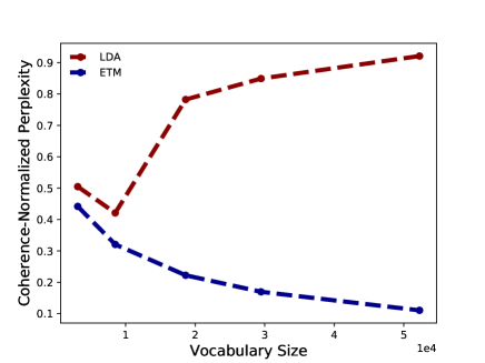
Figure 1: Ratio of the normalized held-out perplexity for document completion and the topic coherence as as a function of the vocabulary size for the etm and lda. While the performance of lda deteriorates for large vocabularies, the etm maintains good performance.

Like lda, the etm is a generative probabilistic model: each document is a mixture of topics and each observed word is assigned to a particular topic. In contrast to lda, the per-topic conditional probability of a term has a log-linear form that involves a low-dimensional representation of the vocabulary. Each term is represented by an embedding; each topic is a point in that embedding space; and the topic’s distribution over terms is proportional to the exponentiated inner product of the topic’s embedding and each term’s embedding. Figures 2 and 3 show topics from a $300$-topic etm of The New York Times. The figures show each topic’s embedding and its closest words; these topics are about Christianity and sports.

Due to the topic representation in terms of a point in the embedding space, the etm is also robust to the presence of stop words, unlike most common topic models. When stop words are included in the vocabulary, the etm assigns topics to the corresponding area of the embedding space (we demonstrate this in Section 6).

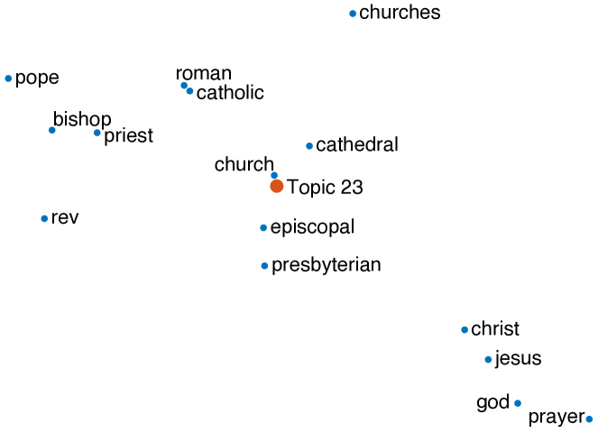
Figure 2: A topic about Christianity found by the etm on The New York Times. The topic is a point in the word embedding space.

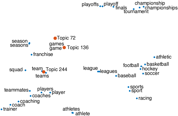
Figure 3: Topics about sports found by the etm. Each topic is a point in the word embedding space.

As for most topic models, the posterior of the topic proportions is intractable to compute. We derive an efficient algorithm for approximating the posterior with variational inference (Jordan et al., 1999; Hoffman et al., 2013; Blei et al., 2017) and additionally use amortized inference to efficiently approximate the topic proportions (Kingma and Welling, 2014; Rezende et al., 2014). The resulting algorithm fits the etm to large corpora with large vocabularies. The algorithm for the etm can either use previously fitted word embeddings, or fit them jointly with the rest of parameters. (In particular, Figures 1 to 3 were obtained with the version of the etm that obtains pre-fitted skip-gram word embeddings.)

We compared the performance of the etm to lda and the neural variational document model (nvdm), a form of multinomial matrix factorization. The etm provides good predictive performance, as measured by held-out log-likelihood on a document completion task (Wallach et al., 2009). It also provides meaningful topics, as measured by topic coherence (Mimno et al., 2011) and topic diversity, a metric that also indicates the quality of the topics. The etm is especially robust to large vocabularies.

2 Related Work

This work develops a new topic model that extends lda. lda has been extended in many ways, and topic modeling has become a subfield of its own. For a review, see Blei (2012) and Boyd-Graber et al. (2017).

One of the goals in developing the etm is to incorporate word similarity into the topic model, and there is previous research that shares this goal. These methods either modify the topic priors (Petterson et al., 2010; Zhao et al., 2017b; Shi et al., 2017; Zhao et al., 2017a) or the topic assignment priors (Xie et al., 2015). For example Petterson et al. (2010) use a word similarity graph (as given by a thesaurus) to bias lda towards assigning similar words to similar topics. As another example, Xie et al. (2015) model the per-word topic assignments of lda using a Markov random field to account for both the topic proportions and the topic assignments of similar words. These methods use word similarity as a type of “side information” about language; in contrast, the etm directly models the similarity (via embeddings) in its generative process of words.

Other work has extended lda to directly involve word embeddings. One common strategy is to convert the discrete text into continuous observations of embeddings, and then adapt lda to generate real-valued data (Das et al., 2015; Xun et al., 2016; Batmanghelich et al., 2016; Xun et al., 2017). With this strategy, topics are Gaussian distributions with latent means and covariances, and the likelihood over the embeddings is modeled with a Gaussian (Das et al., 2015) or a Von-Mises Fisher distribution (Batmanghelich et al., 2016). The etm differs from these approaches in that it is a model of categorical data, one that goes through the embeddings matrix. Thus it does not require pre-fitted embeddings and, indeed, can learn embeddings as part of its inference process.

There have been a few other ways of combining lda and embeddings. Nguyen et al. (2015) mix the likelihood defined by lda with a log-linear model that uses pre-fitted word embeddings; Bunk and Krestel (2018) randomly replace words drawn from a topic with their embeddings drawn from a Gaussian; and Xu et al. (2018) adopt a geometric perspective, using Wasserstein distances to learn topics and word embeddings jointly.

Another thread of recent research improves topic modeling inference through deep neural networks (Srivastava and Sutton, 2017; Card et al., 2017; Cong et al., 2017; Zhang et al., 2018). Specifically, these methods reduce the dimension of the text data through amortized inference and the variational auto-encoder (Kingma and Welling, 2014; Rezende et al., 2014). To perform inference in the etm, we also avail ourselves of amortized inference methods (Gershman and Goodman, 2014).

Finally, as a document model, the etm also relates to works that learn per-document representations as part of an embedding model (Le and Mikolov, 2014; Moody, 2016; Miao et al., 2016). In contrast to these works, the document variables in the etm are part of a larger probabilistic topic model.

3 Background

The etm builds on two main ideas, lda and word embeddings. Consider a corpus of $D$ documents, where the vocabulary contains $V$ distinct terms. Let $w_{dn}\in\{1,\ldots,V\}$ denote the $n^{\textrm{th}}$ word in the $d^{\textrm{th}}$ document.

Latent Dirichlet allocation.  lda is a probabilistic generative model of documents (Blei et al., 2003). It posits $K$ topics $\beta_{1:K}$, each of which is a distribution over the vocabulary. lda assumes each document comes from a mixture of topics, where the topics are shared across the corpus and the mixture proportions are unique for each document. The generative process for each document is the following:

1. Draw topic proportion $\theta_{d}\sim\textrm{Dirichlet}(\alpha_{\theta})$.

2. For each word $n$ in the document:

   1. Draw topic assignment $z_{dn}\sim\text{Cat}(\theta_{d})$.

   2. Draw word $w_{dn}\sim\text{Cat}(\beta_{z_{dn}})$.

Here, Cat$(\cdot)$ denotes the categorical distribution. lda places a Dirichlet prior on the topics, $\beta_{k}\sim\textrm{Dirichlet}(\alpha_{\beta})$ for $k=1,\ldots,K$. The concentration parameters $\alpha_{\beta}$ and $\alpha_{\theta}$ of the Dirichlet distributions are fixed model hyperparameters.

Word embeddings.  Word embeddings provide models of language that use vector representations of words (Rumelhart and Abrahamson, 1973; Bengio et al., 2003). The word representations are fitted to relate to meaning, in that words with similar meanings will have representations that are close. (In embeddings, the “meaning” of a word comes from the contexts in which it is used.)

We focus on the continuous bag-of-words (cbow) variant of word embeddings (Mikolov et al., 2013b). In cbow, the likelihood of each word $w_{dn}$ is

$$w_{dn}\sim\textrm{softmax}(\rho^{\top}\alpha_{dn}).$$ (1)

The embedding matrix $\rho$ is a $L\times V$ matrix whose columns contain the embedding representations of the vocabulary, $\rho_{v}\in\mathbb{R}^{L}$. The vector $\alpha_{dn}$ is the context embedding. The context embedding is the sum of the context embedding vectors ($\alpha_{v}$ for each word $v$) of the words surrounding $w_{dn}$.

4 The Embedded Topic Model

The etm is a topic model that uses embedding representations of both words and topics. It contains two notions of latent dimension. First, it embeds the vocabulary in an $L$-dimensional space. These embeddings are similar in spirit to classical word embeddings. Second, it represents each document in terms of $K$ latent topics.

In traditional topic modeling, each topic is a full distribution over the vocabulary. In the etm, however, the $k^{\textrm{th}}$ topic is a vector $\alpha_{k}\in\mathbb{R}^{L}$ in the embedding space. We call $\alpha_{k}$ a topic embedding—it is a distributed representation of the $k^{\textrm{th}}$ topic in the semantic space of words.

In its generative process, the etm uses the topic embedding to form a per-topic distribution over the vocabulary. Specifically, the etm uses a log-linear model that takes the inner product of the word embedding matrix and the topic embedding. With this form, the etm assigns high probability to a word $v$ in topic $k$ by measuring the agreement between the word’s embedding and the topic’s embedding.

Denote the $L\times V$ word embedding matrix by $\rho$; the column $\rho_{v}$ is the embedding of $v$. Under the etm, the generative process of the $d^{\textrm{th}}$ document is the following:

• Draw topic proportions $\theta_{d}\sim\mathcal{LN}(0,I).$

• For each word $n$ in the document:

  • Draw topic assignment $z_{dn}\sim\text{Cat}(\theta_{d}).$

  • Draw the word $w_{dn}\sim\text{softmax}(\rho^{\top}\alpha_{z_{dn}})$.

In Step 1, $\mathcal{LN}(\cdot)$ denotes the logistic-normal distribution (Aitchison and Shen, 1980; Blei and Lafferty, 2007); it transforms a standard Gaussian random variable to the simplex. A draw $\theta_{d}$ from this distribution is obtained as

$$\delta_{d}\sim\mathcal{N}\left(0,I\right);\quad\theta_{d}=\text{softmax}(\delta_{d}).$$ (2)

(We replaced the Dirichlet with the logistic normal to more easily use reparameterization in the inference algorithm; see Section 5.)

Steps 1 and 2a are standard for topic modeling: they represent documents as distributions over topics and draw a topic assignment for each observed word. Step 2b is different; it uses the embeddings of the vocabulary $\rho$ and the assigned topic embedding $\alpha_{z_{dn}}$ to draw the observed word from the assigned topic, as given by $z_{dn}$.

The topic distribution in Step 2b mirrors the cbow likelihood in Eq. 1. Recall cbow uses the surrounding words to form the context vector $\alpha_{dn}$. In contrast, the etm uses the topic embedding $\alpha_{z_{dn}}$ as the context vector, where the assigned topic $z_{dn}$ is drawn from the per-document variable $\theta_{d}$. The etm draws its words from a document context, rather than from a window of surrounding words.

The etm likelihood uses a matrix of word embeddings $\rho$, a representation of the vocabulary in a lower dimensional space. In practice, it can either rely on previously fitted embeddings or learn them as part of its overall fitting procedure. When the etm learns the embeddings as part of the fitting procedure, it simultaneously finds topics and an embedding space.

When the etm uses previously fitted embeddings, it learns the topics of a corpus in a particular embedding space. This strategy is particularly useful when there are words in the embedding that are not used in the corpus. The etm can hypothesize how those words fit in to the topics because it can calculate $\rho_{v}^{\top}\alpha_{k}$, even for words $v$ that do not appear in the corpus.

5 Inference and Estimation

We are given a corpus of documents $\{\mathbf{w}_{1},\ldots,\mathbf{w}_{D}\}$, where $\mathbf{w}_{d}$ is a collection of $N_{d}$ words. How do we fit the etm?

The marginal likelihood.  The parameters of the etm are the embeddings $\rho_{1:V}$ and the topic embeddings $\alpha_{1:K}$; each $\alpha_{k}$ is a point in the embedding space. We maximize the marginal likelihood of the documents,

$$\mathcal{L}(\alpha,\rho)=\sum_{d=1}^{D}\log p(\mathbf{w}_{d}\,|\,\alpha,\rho).$$ (3)

The problem is that the marginal likelihood of each document is intractable to compute. It involves a difficult integral over the topic proportions, which we write in terms of the untransformed proportions $\delta_{d}$ in Eq. 2,

$$p(\mathbf{w}_{d}\,|\,\alpha,\rho)=\int p(\delta_{d})\prod_{n=1}^{N_{d}}p(w_{dn}\,|\,\delta_{d},\alpha,\rho)\,\mathrm{d}\delta_{d}.$$ (4)

The conditional distribution of each word marginalizes out the topic assignment $z_{dn}$,

$$p(w_{dn}\,|\,\delta_{d},\alpha,\rho) =\sum_{k=1}^{K}\theta_{dk}\beta_{k,w_{dn}}.$$ (5)

Here, $\theta_{dk}$ denotes the (transformed) topic proportions (Eq. 2) and $\beta_{kv}$ denotes a traditional “topic,” i.e., a distribution over words, induced by the word embeddings $\rho$ and the topic embedding $\alpha_{k}$,

$$\beta_{kv}=\textrm{softmax}(\rho^{\top}\alpha_{k})\big{|}_{v}.$$ (6)

Eqs. 4 to 6 flesh out the likelihood in Eq. 3.

Variational inference.  We sidestep the intractable integral with variational inference (Jordan et al., 1999; Blei et al., 2017). Variational inference optimizes a sum of per-document bounds on the log of the marginal likelihood of Eq. 4. There are two sets of parameters to optimize: the model parameters, as described above, and the variational parameters, which tighten the bounds on the marginal likelihoods.

To begin, posit a family of distributions of the untransformed topic proportions $q(\delta_{d}\,;\,\mathbf{w}_{d},\nu)$. We use amortized inference, where the variational distribution of $\delta_{d}$ depends on both the document $\mathbf{w}_{d}$ and shared variational parameters $\nu$. In particular $q(\delta_{d}\,;\,\mathbf{w}_{d},\nu)$ is a Gaussian whose mean and variance come from an “inference network,” a neural network parameterized by $\nu$ (Kingma and Welling, 2014). The inference network ingests the document $\mathbf{w}_{d}$ and outputs a mean and variance of $\delta_{d}$. (To accommodate documents of varying length, we form the input of the inference network by normalizing the bag-of-word representation of the document by the number of words $N_{d}$.)

We use this family of variational distributions to bound the log-marginal likelihood. The evidence lower bound (elbo) is a function of the model parameters and the variational parameters,

$$\mathcal{L}(\alpha,\rho,\nu) =\sum_{d=1}^{D}\sum_{n=1}^{N_{d}}\mathbb{E}_{q}\left[\log p(w_{nd}\,|\,\delta_{d},\rho,\alpha)\right]$$

$$-\sum_{d=1}^{D}\mathrm{KL}(q(\delta_{d};\mathbf{w}_{d},\nu)\;||\;p(\delta_{d})).$$ (7)

As a function of the variational parameters, the first term encourages them to place mass on topic proportions $\delta_{d}$ that explain the observed words; the second term encourages them to be close to the prior $p(\delta_{d})$. As a function of the model parameters, this objective maximizes the expected complete log-likelihood, $\sum_{d}\log p(\delta_{d},\mathbf{w}_{d}\,|\,\alpha,\rho)$.

We optimize the elbo with respect to both the model parameters and the variational parameters. We use stochastic optimization, forming noisy gradients by taking Monte Carlo approximations of the full gradient through the reparameterization trick (Kingma and Welling, 2014; Titsias and Lázaro-Gredilla, 2014; Rezende et al., 2014). We also use data subsampling to handle large collections of documents (Hoffman et al., 2013). We set the learning rate with Adam (Kingma and Ba, 2015). The procedure is shown in Algorithm 1, where the notation $\textrm{NN}(\mathbf{x}\,;\,\nu)$ represents a neural network with input $\mathbf{x}$ and parameters $\nu$.

Algorithm 1 Topic modeling with the etm

  Initialize model and variational parameters

  for iteration $i=1,2,\ldots$ do

     Compute $\beta_{k}=\text{softmax}(\rho^{\top}\alpha_{k})$ for each topic $k$

     Choose a minibatch $\mathcal{B}$ of documents

     for each document $d$ in $\mathcal{B}$ do

        Get normalized bag-of-word representat. $\mathbf{x}_{d}$

        Compute $\mu_{d}=\textrm{NN}(\mathbf{x}_{d}\,;\,\nu_{\mu})$

        Compute $\Sigma_{d}=\textrm{NN}(\mathbf{x}_{d}\,;\,\nu_{\Sigma})$

        Sample $\theta_{d}\sim\mathcal{L}\mathcal{N}(\mu_{d},\Sigma_{d})$

        for each word in the document do

           Compute $p(w_{dn}\,|\,\theta_{d})=\theta_{d}^{\top}\beta_{\cdot,w_{dn}}$

        end for

     end for

     Estimate the elbo and its gradient (backprop.)

     Update model parameters $\alpha_{1:K}$

     Update variational parameters ($\nu_{\mu}$, $\nu_{\Sigma}$)

  end for

6 Empirical Study

Table 1: Word embeddings learned by all document models (and skip-gram) on the New York Times with vocabulary size $118{,}363$.

Skip-gram embeddings etm embeddings love family woman politics love family woman politics loved families man political joy children girl political passion grandparents girl religion loves son boy politician loves mother boy politicking loved mother mother ideology affection friends teenager ideology passion father daughter speeches adore relatives person partisanship wonderful wife pregnant ideological nvdm embeddings $\Delta$-nvdm embeddings love family woman politics love family woman politics loves sons girl political miss home life political passion life women politician young father marriage faith wonderful brother man politicians born son women marriage joy son pregnant politically dream day read politicians beautiful lived boyfriend democratic younger mrs young election

Table 2: Top five words of seven most used topics from different document models on $1.8$M documents of the New York Times corpus with vocabulary size $212{,}237$ and $K=300$ topics.

LDA
time	year	officials	mr	city	percent	state
day	million	public	president	building	million	republican
back	money	department	bush	street	company	party
good	pay	report	white	park	year	bill
long	tax	state	clinton	house	billion	mr
nvdm
scholars	japan	gansler	spratt	assn	ridership	pryce
gingrich	tokyo	wellstone	tabitha	assoc	mtv	mickens
funds	pacific	mccain	mccorkle	qtr	straphangers	mckechnie
institutions	europe	shalikashvili	cheetos	yr	freierman	mfume
endowment	zealand	coached	vols	nyse	riders	filkins
$\Delta$-nvdm
concerto	servings	nato	innings	treas	patients	democrats
solos	tablespoons	soviet	scored	yr	doctors	republicans
sonata	tablespoon	iraqi	inning	qtr	medicare	republican
melodies	preheat	gorbachev	shutout	outst	dr	senate
soloist	minced	arab	scoreless	telerate	physicians	dole
Labeled etm
music	republican	yankees	game	wine	court	company
dance	bush	game	points	restaurant	judge	million
songs	campaign	baseball	season	food	case	stock
opera	senator	season	team	dishes	justice	shares
concert	democrats	mets	play	restaurants	trial	billion
etm
game	music	united	wine	company	yankees	art
team	mr	israel	food	stock	game	museum
season	dance	government	sauce	million	baseball	show
coach	opera	israeli	minutes	companies	mets	work
play	band	mr	restaurant	billion	season	artist

We study the performance of the etm and compare it to other unsupervised document models. A good document model should provide both coherent patterns of language and an accurate distribution of words, so we measure performance in terms of both predictive accuracy and topic interpretability. We measure accuracy with log-likelihood on a document completion task (Rosen-Zvi et al., 2004; Wallach et al., 2009); we measure topic interpretability as a blend of topic coherence and diversity. We find that, of the interpretable models, the etm is the one that provides better predictions and topics.

In a separate analysis (Section 6.1), we study the robustness of each method in the presence of stop words. Standard topic models fail in this regime—since stop words appear in many documents, every learned topic includes some stop words, leading to poor topic interpretability. In contrast, the etm is able to use the information from the word embeddings to provide interpretable topics.

Corpora.  We study the 20Newsgroups corpus and the New York Times corpus.

The 20Newsgroup corpus is a collection of newsgroup posts. We preprocess the corpus by filtering stop words, words with document frequency above 70%, and tokenizing. To form the vocabulary, we keep all words that appear in more than a certain number of documents, and we vary the threshold from 100 (a smaller vocabulary, where $V=3{,}102$) to 2 (a larger vocabulary, where $V=52{,}258$). After preprocessing, we further remove one-word documents from the validation and test sets. We split the corpus into a training set of $11{,}260$ documents, a test set of $7{,}532$ documents, and a validation set of $100$ documents.

The New York Times corpus is a larger collection of news articles. It contains more than $1.8$ million articles, spanning the years 1987–2007. We follow the same preprocessing steps as for 20Newsgroups. We form versions of this corpus with vocabularies ranging from $V=5{,}921$ to $V=212{,}237$. After preprocessing, we use $85\%$ of the documents for training, $10\%$ for testing, and $5\%$ for validation.

Models.  We compare the performance of the etm with two other document models: latent Dirichlet allocation (lda) and the neural variational document model (nvdm).

lda (Blei et al., 2003) is a standard topic model that posits Dirichlet priors for the topics $\beta_{k}$ and topic proportions $\theta_{d}$. (We set the prior hyperparameters to $1$.) It is a conditionally conjugate model, amenable to variational inference with coordinate ascent. We consider lda because it is the most commonly used topic model, and it has a similar generative process as the etm.

The nvdm (Miao et al., 2016) is a multinomial factor model of documents; it posits the likelihood $w_{dn}\sim\text{softmax}(\beta^{\top}\theta_{d})$, where the $K$-dimensional vector $\theta_{d}\sim\mathcal{N}(\mathbf{0},\mathbf{I}_{K})$ is a per-document variable, and $\beta$ is a real-valued matrix of size $K\times V$. The nvdm uses a per-document real-valued latent vector $\theta_{d}$ to average over the embedding matrix $\beta$ in the logit space. Like the etm, the nvdm uses amortized variational inference to jointly learn the approximate posterior over the document representation $\theta_{d}$ and the model parameter $\beta$.

nvdm is not interpretable as a topic model; its latent variables are unconstrained. We study a more interpretable variant of the nvdm which constrains $\theta_{d}$ to lie in the simplex, replacing its Gaussian prior with a logistic normal (Aitchison and Shen, 1980). (This can be thought of as a semi-nonnegative matrix factorization.) We call this document model $\Delta$-nvdm.

We study two variants of the etm, one where the word embeddings are pre-fitted and one where they are learned jointly with the rest of the parameters. The variant with pre-fitted embeddings is called the “labeled etm.” We use skip-gram embeddings (Mikolov et al., 2013b).

Algorithm settings.  Given a corpus, each model comes with an approximate posterior inference problem. We use variational inference for all of the models and employ stochastic variational inference (svi) (Hoffman et al., 2013) to speed up the optimization. The minibatch size is $1{,}000$ documents. For lda, we set the learning rate as suggested by Hoffman et al. (2013): the delay is $10$ and the forgetting factor is $0.85$.

Within svi, lda enjoys coordinate ascent variational updates, with $5$ inner steps to optimize the local variables. For the other models, we use amortized inference over the local variables $\theta_{d}$. We use $3$-layer inference networks and we set the local learning rate to $0.002$. We use $\ell_{2}$ regularization on the variational parameters (the weight decay parameter is $1.2\times 10^{-6}$).

(a) Topic quality as measured by normalized product of topic coherence and topic diversity (the higher the better) vs. predictive performance as measured by normalized log-likelihood on document completion (the higher the better) on the 20NewsGroup dataset.

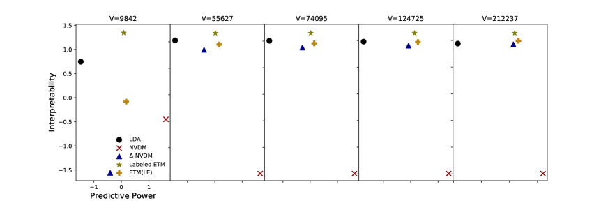
(b) Topic quality as measured by normalized product of topic coherence and topic diversity (the higher the better) vs. predictive performance as measured by normalized log-likelihood on document completion (the higher the better) on the New York Times dataset.

Figure 4: Performance on the 20NewsGroups and the New York Times datasets for different vocabulary sizes. On both plots, better models are on the top right corner. Overall, the etm is a better topic model.

Qualitative results.  We first examine the embeddings. The etm, nvdm, and $\Delta$-nvdm all involve a word embedding. We illustrate them by fixing a set of terms and calculating the words that occur in the neighborhood around them. For comparison, we also illustrate word embeddings learned by the skip-gram model.

Table 1 illustrates the embeddings of the different models. All the methods provide interpretable embeddings—words with related meanings are close to each other. The etm and the nvdm learn embeddings that are similar to those from the skip-gram. The embeddings of $\Delta$-nvdm are different; the simplex constraint on the local variable changes the nature of the embeddings.

We next look at the learned topics. Table 6 displays the $7$ most used topics for all methods, as given by the average of the topic proportions $\theta_{d}$. lda and the etm both provide interpretable topics. Neither nvdm nor $\Delta$-nvdm provide interpretable topics; their model parameters $\beta$ are not interpretable as distributions over the vocabulary that mix to form documents.

Quantitative results.  We next study the models quantitatively. We measure the quality of the topics and the predictive performance of the model. We found that among models with interpretable topics, the etm provides the best predictions.

We measure topic quality by blending two metrics: topic coherence and topic diversity. Topic coherence is a quantitative measure of the interpretability of a topic (Mimno et al., 2011). It is the average pointwise mutual information of two words drawn randomly from the same document (Lau et al., 2014),

$$\textrm{TC}=\frac{1}{K}\sum_{k=1}^{K}\frac{1}{45}\sum_{i=1}^{10}\sum_{j=i+1}^{10}f(w_{i}^{(k)},w_{j}^{(k)}),$$

where $\{w_{1}^{(k)},\ldots,w_{10}^{(k)}\}$ denotes the top-$10$ most likely words in topic $k$. Here, $f(\cdot,\cdot)$ is the normalized pointwise mutual information,

$$f(w_{i},w_{j})=\frac{\log\frac{P(w_{i},w_{j})}{P(w_{i})P(w_{j})}}{-\log P(w_{i},w_{j})}.$$

The quantity $P(w_{i},w_{j})$ is the probability of words $w_{i}$ and $w_{j}$ co-occurring in a document and $P(w_{i})$ is the marginal probability of word $w_{i}$. We approximate these probabilities with empirical counts.

The idea behind topic coherence is that a coherent topic will display words that tend to occur in the same documents. In other words, the most likely words in a coherent topic should have high mutual information. Document models with higher topic coherence are more interpretable topic models.

We combine coherence with a second metric, topic diversity. We define topic diversity to be the percentage of unique words in the top $25$ words of all topics. Diversity close to $0$ indicates redundant topics; diversity close to $1$ indicates more varied topics. We define the overall metric for the quality of a model’s topics as the product of its topic diversity and topic coherence.

A good topic model also provides a good distribution of language. To measure predictive quality, we calculate log likelihood on a document completion task (Rosen-Zvi et al., 2004; Wallach et al., 2009). We divide each test document into two sets of words. The first half is observed: it induces a distribution over topics which, in turn, induces a distribution over the next words in the document. We then evaluate the second half under this distribution. A good document model should provide higher log-likelihood on the second half. (For all methods, we approximate the likelihood by setting $\theta_{d}$ to the variational mean.)

We study both corpora and with different vocabularies. Figure 4 shows topic quality as a function of predictive power. (To ease visualization, we normalize both metrics by subtracting the mean and dividing by the standard deviation.) The best models are on the upper right corner.

lda predicts worst in almost all settings. On 20NewsGroups, the nvdm’s predictions are in general better than lda but worse than for the other methods; on the New York Times, the nvdm gives the best predictions. However, topic quality for the nvdm is far below the other methods. (It does not provide “topics”, so we assess the interpretability of its $\beta$ matrix.) In prediction, both versions of the etm are at least as good as the simplex-constrained $\Delta$-nvdm.

These figures show that, of the interpretable models, the etm provides the best predictive performance while keeping interpretable topics. It is robust to large vocabularies.

6.1 Stop words

We now study a version of the New York Times corpus that includes all stop words. We remove infrequent words to form a vocabulary of size $10{,}283$. Our goal is to show that the labeled etm provides interpretable topics even in the presence of stop words, another regime where topic models typically fail. In particular, given that stop words appear in many documents, traditional topic models learn topics that contain stop words, regardless of the actual semantics of the topic. This leads to poor topic interpretability.

We fit lda, the $\Delta$-nvdm, and the labeled etm with $K=300$ topics. (We do not report the nvdm because it does not provide interpretable topics.) Table 3 shows topic quality (the product of topic coherence and topic diversity). Overall, the labeled etm gives the best performance in terms of topic quality.

While the etm has a few “stop topics” that are specific for stop words (see, e.g., Figure 5), $\Delta$-nvdm and lda have stop words in almost every topic. (The topics are not displayed here for space constraints.) The reason is that stop words co-occur in the same documents as every other word; therefore traditional topic models have difficulties telling apart content words and stop words. The labeled etm recognizes the location of stop words in the embedding space; its sets them off on their own topic.

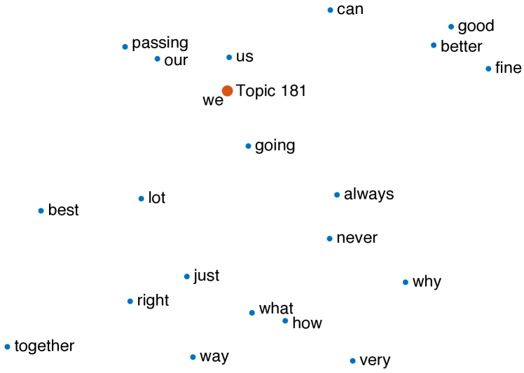
Figure 5: A topic containing stop words found by the etm on The New York Times. The etm is robust even in the presence of stop words.

7 Conclusion

We developed the etm, a generative model of documents that marries lda with word embeddings. The etm assumes that topics and words live in the same embedding space, and that words are generated from a categorical distribution whose natural parameter is the inner product of the word embeddings and the embedding of the assigned topic.

The etm learns interpretable word embeddings and topics, even in corpora with large vocabularies. We studied the performance of the etm against several document models. The etm learns both coherent patterns of language and an accurate distribution of words.

Table 3: Topic quality on the New York Times data in the presence of stop words. Topic quality is the product of topic coherence and topic diversity (higher is better). The labeled etm is robust to stop words; it achieves similar topic coherence than when there are no stop words.

	Coherence	Diversity	Quality
lda	$0.13$	$0.14$	$0.0173$
$\Delta$-nvdm	$0.17$	$0.11$	$0.0187$
Labeled etm	$\mathbf{0.18}$	$\mathbf{0.22}$	$\mathbf{0.0405}$

References

- Aitchison and Shen (1980) J. Aitchison and S. Shen. 1980. Logistic normal distributions: Some properties and uses. Biometrika, 67(2):261–272.
- Batmanghelich et al. (2016) K. Batmanghelich, A. Saeedi, K. Narasimhan, and S. Gershman. 2016. Nonparametric spherical topic modeling with word embeddings. In Proceedings of the conference. Association for Computational Linguistics. Meeting, volume 2016, page 537. NIH Public Access.
- Bengio et al. (2003) Y. Bengio, R. Ducharme, P. Vincent, and C. Janvin. 2003. A neural probabilistic language model. Journal of Machine Learning Research, 3:1137–1155.
- Bengio et al. (2006) Y. Bengio, H. Schwenk, J.-S. Senécal, F. Morin, and J.-L. Gauvain. 2006. Neural probabilistic language models. In Innovations in Machine Learning, pages 137–186. Springer.
- Blei (2012) D. M. Blei. 2012. Probabilistic topic models. Communications of the ACM, 55(4):77–84.
- Blei et al. (2017) D. M. Blei, A. Kucukelbir, and J. D. McAuliffe. 2017. Variational inference: A review for statisticians. Journal of the American Statistical Association, 112(518):859–877.
- Blei and Lafferty (2007) D. M. Blei and J. D. Lafferty. 2007. A correlated topic model of Science. The Annals of Applied Statistics, 1(1):17–35.
- Blei et al. (2003) D. M. Blei, A. Y. Ng, and M. I. Jordan. 2003. Latent dirichlet allocation. Journal of machine Learning research, 3(Jan):993–1022.
- Boyd-Graber et al. (2017) J. Boyd-Graber, Y. Hu, and D. Mimno. 2017. Applications of topic models. Foundations and Trends in Information Retrieval, 11(2–3):143–296.
- Bunk and Krestel (2018) S. Bunk and R. Krestel. 2018. Welda: Enhancing topic models by incorporating local word context. In Proceedings of the 18th ACM/IEEE on Joint Conference on Digital Libraries, pages 293–302. ACM.
- Card et al. (2017) D. Card, C. Tan, and N. A. Smith. 2017. A neural framework for generalized topic models. In arXiv:1705.09296.
- Cong et al. (2017) Y. Cong, B. Chen, H. Liu, and M. Zhou. 2017. Deep latent Dirichlet allocation with topic-layer-adaptive stochastic gradient Riemannian MCMC. In International Conference on Machine Learning.
- Das et al. (2015) R. Das, M. Zaheer, and C. Dyer. 2015. Gaussian LDA for topic models with word embeddings. In Association for Computational Linguistics and International Joint Conference on Natural Language Processing (Volume 1: Long Papers).
- Gershman and Goodman (2014) S. J. Gershman and N. D. Goodman. 2014. Amortized inference in probabilistic reasoning. In Annual Meeting of the Cognitive Science Society.
- Hoffman et al. (2010) M. D. Hoffman, D. M. Blei, and F. Bach. 2010. Online learning for latent Dirichlet allocation. In Advances in Neural Information Processing Systems.
- Hoffman et al. (2013) M. D. Hoffman, D. M. Blei, C. Wang, and J. Paisley. 2013. Stochastic variational inference. Journal of Machine Learning Research, 14:1303–1347.
- Jordan et al. (1999) M. I. Jordan, Z. Ghahramani, T. S. Jaakkola, and L. K. Saul. 1999. An introduction to variational methods for graphical models. Machine Learning, 37(2):183–233.
- Kingma and Ba (2015) D. P. Kingma and J. L. Ba. 2015. Adam: A method for stochastic optimization. In International Conference on Learning Representations.
- Kingma and Welling (2014) D. P. Kingma and M. Welling. 2014. Auto-encoding variational Bayes. In International Conference on Learning Representations.
- Lau et al. (2014) J. H. Lau, D. Newman, and T. Baldwin. 2014. Machine reading tea leaves: Automatically evaluating topic coherence and topic model quality. In Conference of the European Chapter of the Association for Computational Linguistics.
- Le and Mikolov (2014) Q. Le and T. Mikolov. 2014. Distributed representations of sentences and documents. In International Conference on Machine Learning.
- Levy and Goldberg (2014) O. Levy and Y. Goldberg. 2014. Neural word embedding as implicit matrix factorization. In Neural Information Processing Systems, pages 2177–2185.
- Li and Tao (2018) Y. Li and Y. Tao. 2018. Word Embedding for Understanding Natural Language: A Survey. Springer International Publishing.
- Miao et al. (2016) Y. Miao, L. Yu, and P. Blunsom. 2016. Neural variational inference for text processing. In International Conference on Machine Learning.
- Mikolov et al. (2013a) T. Mikolov, K. Chen, G. Corrado, and J. Dean. 2013a. Efficient estimation of word representations in vector space. ICLR Workshop Proceedings. arXiv:1301.3781.
- Mikolov et al. (2013b) T. Mikolov, I. Sutskever, K. Chen, G. S. Corrado, and J. Dean. 2013b. Distributed representations of words and phrases and their compositionality. In Neural Information Processing Systems, pages 3111–3119.
- Mimno et al. (2011) D. Mimno, H. M. Wallach, E. Talley, M. Leenders, and A. McCallum. 2011. Optimizing semantic coherence in topic models. In Conference on Empirical Methods in Natural Language Processing.
- Mnih and Kavukcuoglu (2013) A. Mnih and K. Kavukcuoglu. 2013. Learning word embeddings efficiently with noise-contrastive estimation. In Neural Information Processing Systems, pages 2265–2273.
- Moody (2016) C. E. Moody. 2016. Mixing dirichlet topic models and word embeddings to make lda2vec. arXiv preprint arXiv:1605.02019.
- Nguyen et al. (2015) D. Q. Nguyen, R. Billingsley, L. Du, and M. Johnson. 2015. Improving topic models with latent feature word representations. Transactions of the Association for Computational Linguistics, 3:299–313.
- Pennington et al. (2014) J. Pennington, R. Socher, and C. D. Manning. 2014. Glove: Global vectors for word representation. In Conference on Empirical Methods on Natural Language Processing, volume 14, pages 1532–1543.
- Petterson et al. (2010) J. Petterson, W. Buntine, S. M. Narayanamurthy, T. S. Caetano, and A. J. Smola. 2010. Word features for latent dirichlet allocation. In Advances in Neural Information Processing Systems, pages 1921–1929.
- Rezende et al. (2014) D. J. Rezende, S. Mohamed, and D. Wierstra. 2014. Stochastic backpropagation and approximate inference in deep generative models. arXiv preprint arXiv:1401.4082.
- Rosen-Zvi et al. (2004) M. Rosen-Zvi, T. Griffiths, M. Steyvers, and P. Smyth. 2004. The author-topic model for authors and documents. In Uncertainty in Artificial Intelligence.
- Rudolph et al. (2016) M. Rudolph, F. J. R. Ruiz, S. Mandt, and D. M. Blei. 2016. Exponential family embeddings. In Advances in Neural Information Processing Systems.
- Rumelhart and Abrahamson (1973) D. Rumelhart and A. Abrahamson. 1973. A model for analogical reasoning. Cognitive Psychology, 5(1):1–28.
- Shi et al. (2017) B. Shi, W. Lam, S. Jameel, S. Schockaert, and K. P. Lai. 2017. Jointly learning word embeddings and latent topics. In Proceedings of the 40th International ACM SIGIR Conference on Research and Development in Information Retrieval, pages 375–384. ACM.
- Srivastava and Sutton (2017) A. Srivastava and C. Sutton. 2017. Autoencoding variational inference for topic models. arXiv preprint arXiv:1703.01488.
- Titsias and Lázaro-Gredilla (2014) M. K. Titsias and M. Lázaro-Gredilla. 2014. Doubly stochastic variational Bayes for non-conjugate inference. In International Conference on Machine Learning.
- Wallach et al. (2009) H. M. Wallach, I. Murray, R. Salakhutdinov, and D. Mimno. 2009. Evaluation methods for topic models. In International Conference on Machine Learning.
- Xie et al. (2015) P. Xie, D. Yang, and E. Xing. 2015. Incorporating word correlation knowledge into topic modeling. In Proceedings of the 2015 conference of the north American chapter of the association for computational linguistics: human language technologies, pages 725–734.
- Xu et al. (2018) H. Xu, W. Wang, W. Liu, and L. Carin. 2018. Distilled Wasserstein learning for word embedding and topic modeling. In Advances in Neural Information Processing Systems.
- Xun et al. (2016) G. Xun, V. Gopalakrishnan, F. Ma, Y. Li, J. Gao, and A. Zhang. 2016. Topic discovery for short texts using word embeddings. In 2016 IEEE 16th international conference on data mining (ICDM), pages 1299–1304. IEEE.
- Xun et al. (2017) G. Xun, Y. Li, W. X. Zhao, J. Gao, and A. Zhang. 2017. A correlated topic model using word embeddings. In IJCAI, pages 4207–4213.
- Zhang et al. (2018) H. Zhang, B. Chen, D. Guo, and M. Zhou. 2018. WHAI: Weibull hybrid autoencoding inference for deep topic modeling. In International Conference on Learning Representations.
- Zhao et al. (2017a) H. Zhao, L. Du, and W. Buntine. 2017a. A word embeddings informed focused topic model. In Asian Conference on Machine Learning, pages 423–438.
- Zhao et al. (2017b) H. Zhao, L. Du, W. Buntine, and G. Liu. 2017b. Metalda: A topic model that efficiently incorporates meta information. In 2017 IEEE International Conference on Data Mining (ICDM), pages 635–644. IEEE.