A hydrodynamic approach to electron beam imaging using a Bloch wave representation

Abstract

Calculations of propagating quantum trajectories associated to a wave function provide new insight into quantum processes such as particle scattering and diffraction. Here, hydrodynamic calculations of electron beam imaging under conditions comparable to those of a scanning or transmission electron microscope display the mechanisms behind different commonly investigated diffraction conditions. The Bloch wave method is used to propagate the electron wave function and associated trajectories are computed to map the wave function as it propagates through the material. Simulations of the two-beam condition and the systematic row are performed and electron diffraction is analysed through a real space interpretation of the wave function. In future work, this method can be further coupled with Monte Carlo modelling in order to create all encompassing simulations of electron imaging.

I Introduction

The wave-particle duality of electrons causes a segregation between the types of simulation techniques employed in the field of electron microscopy. Simulations are categorized as either image simulations, where the probability distribution of the electron wave function is used to obtain contour maps relating to the exit plane or diffraction pattern, or particle scattering simulations using classical methods to obtain intensities associated mostly to X-ray emission events and particle penetration Kirkland (2010). Image simulations use techniques such as multislice Allen et al. (2015); den Broek et al. (2015); Dwyer (2010) or Bloch wave Pennycook and Jesson (1990); Winkelmann et al. (2007); Findlay et al. (2003); Rossouw et al. (2003) which simulate the probability density in real or reciprocal space of the electron upon exit of the material. Conversely, scattered particle trajectories are typically simulated through Monte Carlo techniques where electrons are assumed to be classical spheres that undergo a forward scattering random walk process where the scattering and energy loss parameters are calculated by physical models Gauvin et al. (2006); Salvat (2015). As of yet, there is no technique which simultaneously simulates both the wave and particle characteristics of electrons within the confines of an electron microscope.

Here, we couple the Bloch wave representation of the electron wave function with the propagation of quantum trajectories to simulate electron-matter interactions inside a crystalline material under various probing conditions. The quantum trajectory method arises from the hydrodynamic formulation of a quantum process Trahan and Wyatt (2006); Oriols (2007). Given an initial position, the particle will follow a specific path dictated by the wave function. The uncertainty then comes in the choice of the initial position, preserving the non-locality of the method Sanz and Miret-Artés (2012). Such simulations have mostly been performed for particle diffraction experiments and small scale quantum processes Sanz et al. (2010, 2002); Efthymiopoulos et al. (2012). In previous work, the method was applied in 2D to simulate the time-dependent propagation of a Gaussian wave-packet under conditions similar to those of an SEM Rudinsky et al. (2017). It was found however that there were a number of limiting numerical factors, such as the energy bandwidth, grid size, and film thickness, which restricted the applicability of a time-dependent propagation scheme Rudinsky et al. (2017). The algorithm developed in this study constitutes a completely new and different approach. The trajectories are no longer calculated using a spectral decomposition and the split-operator method is substituted for the Bloch wave method. Other work has been done using a multislice approach to simulate a scanning transmission electron microscope (STEM) probe located at different positions along a unit cell Zhang et al. (2015); Zeng and Ding (2011). However, there was little analysis done of the beam interaction with the material, specifically at different probing conditions Zhang et al. (2015). The use of the multislice method also limits usability of the calculation because the trajectories may only be computed within the confines of the chosen grid. An important advantage of the Bloch wave method is the possibility of computing the wave function at any point in space without being restricted to a structured grid. Furthermore, computations may be performed at lower accelerating voltages, making the method applicable for wave function simulations at energies typically used in scanning electron microscopes (SEM) Winkelmann et al. (2007); Picard et al. (2014). With this, Bloch wave calculations coupled with quantum trajectories have been previously investigated by Cheng et al. Cheng et al. (2018). While they displayed computations at normal incidence and simulations of electron backscattered diffraction images (EBSD), criteria such as the number of beams used and the initial wave function of the EBSD computation method were not indicated, making it difficult to reproduce their findings. There was also no explanation of the calculation process used in the EBSD simulations and consequently other, more in depth and reproducible studies, are necessary.

In this study, the electron wave function along the particle path was computed using the Bloch wave expression to simulate electrons travelling through a single crystal of Cu. Simulations were performed at 200 and 30 keV to distinguish the difference in electron transport in TEM versus SEM-like conditions. The initial positions of the trajectories were chosen uniformly to map out the wave function over the entire unit cell. A variety of probing conditions were also investigated, such as the (100) zone axis, the two beam Bragg condition, and the systematic row condition. Trajectory simulations in these conditions provide information to the origins of various contrasts typically observed. The quantum potential and quantum force are also computed at the exit plane. These values represent the quantum effects which cannot be explained through classical particle propagation Trahan and Wyatt (2006). As a result, these parameters show how electron propagation through a crystalline material leads to diffraction phenomena. It is shown through the quantum force that at normal incidence, electrons are drawn to and from the atom columns, resulting in their channelling through the material. This is also seen in the systematic row case where particles between atom columns are drawn towards them causing variations in the edges of the band contrasts.

II Method

A Bloch wave expression was used to compute the electron wave function along the trajectory paths. The wave function, $\Psi(\mathbf{r})$, of an electron in a periodic potential can be expressed as a sum of Bloch waves weighted by excitation coefficients $\alpha_{\mathbf{g}}^{(j)}$ for each Bloch wave $j$ De Graef (2003),

$$\Psi(\mathbf{r})=\sum_{\mathbf{g}}\left(\sum_{j}\alpha_{\mathbf{g}}^{(j)}C_{\mathbf{g}}^{(j)}e^{2\pi i\gamma^{(j)}z}\right)e^{2\pi i(\mathbf{k}_{0}+\mathbf{g})\cdot\mathbf{r}}$$ (1)

The coefficients $C_{\mathbf{g}}^{(j)}$ and contributions $\gamma^{(j)}$ of each Bloch wave are obtained by solving the eigenvalue equation,

$$\mathbf{k}_{0}-(\mathbf{k}^{(j)}-\mathbf{g})C^{(j)}_{\mathbf{g}}+\sum_{\mathbf{h}\neq\mathbf{g}}U_{\mathbf{g}-\mathbf{h}}C^{(j)}_{\mathbf{h}}=2\gamma^{(j)}k_{0}C^{(j)}_{\mathbf{g}}$$ (2)

where $C_{\mathbf{g}}^{(j)}$ are the eigenvectors and $\gamma_{\mathbf{g}}^{(j)}$ are the eigenvalues De Graef (2003). The factors $U_{\mathbf{g}}$ are obtained from the Fourier coefficients, $V_{\mathbf{g}}$, of the electrostatic potential,

$$U_{\mathbf{g}}=\frac{2m_{0}e}{h^{2}}V_{\mathbf{g}}$$ (3)

for a particle of mass $m_{0}$, charge $e$ and where $h$ is Plank’s constant. The Fourier coefficients, $V_{\mathbf{g}}$, were computed using a summation over the pairwise contributions of the $N$ atoms in the unit cell as,

$$V_{\mathbf{g}}=\sum_{\mathbf{n}\in N}f_{\mathbf{g}}e^{-2\pi i(\mathbf{g}\cdot\mathbf{n})}$$ (4)

where $f_{\mathbf{g}}$ is a parametrization of scattering factors tabulated by Kirkland Kirkland (2010).

$$f_{\mathbf{g}}=\sum_{k=1}^{3}\frac{A_{k}}{|\mathbf{g}|^{2}+B_{k}}+C_{k}e^{-D_{k}|\mathbf{g}|^{2}}$$ (5)

This is in contrast to the parametrization of the real space potential utilised in Rudinsky et al. (2017). Here, only the Fourier coefficients of the potential are required. Absorption was not included in the simulations performed in this study, which is why the imaginary term of the electrostatic potential is neglected in the above derivations. Simulations were performed for copper and the values of the parametrization factors in Eq. 5 are displayed in Table 1

Table 1: Parametrization factors for Cu Kirkland (2010)

$A_{k}$ (Å-1)	0.358774531	1.76181348	0.636905053
$B_{k}$ (Å-2)	0.106153463	1.01640995	15.3659093
$C_{k}$ (Å)	0.00744930667	0.189002347	0.229619589
$D_{k}$ (Å2)	0.0385345989	0.398427790	0.901419843

After the beams with zero structure factor were eliminated, Bethe potentials were used to further limit the number of beams required for the computation. Beams are separated into weak and strong beams depending on the following criteria Zuo and Weickenmeier (1995); Wang and Graef (2016); Picard et al. (2014).

$$\frac{|s_{\mathbf{g}}|}{\lambda U_{\mathbf{g}}}\leq c_{s}\mbox{\hskip 14.22636pt(strong)}$$ (6)

$$c_{s}< \frac{|s_{\mathbf{g}}|}{\lambda U_{\mathbf{g}}}\leq c_{w}\mbox{\hskip 14.22636pt(weak)}$$ (7)

where $s_{\mathbf{g}}$ is the excitation error and $\lambda$ is the wave length. Beams that are considered strong are used for the diagonalization, while those that are weak contribute as perturbation factors to the entries of the dynamical matrix. The values $(c_{s},c_{w})$ were chosen to ensure the difference between the full dynamical matrix and the reduced matrix using Bethe potentials was within the order of $10^{-3}$. The difference between the intensities is defined as follows Wang and Graef (2016),

$$\delta I=\sqrt{\frac{1}{N_{s}}\frac{1}{T}\sum_{N_{s}}(I_{\mathbf{g}}^{f}-I_{\mathbf{g}}^{s})^{2}}$$ (8)

where $N_{s}$ is the total number of strong beams, $I_{\mathbf{g}}$ is the intensity of beam $\mathbf{g}$ and $T$ is the maximum thickness used in the calculation. The order of magnitude chosen was done to limit oversampling of the electron wave function. Quantum trajectories are very sensitive to small local perturbations and therefore, in order to simultaneously ensure smoothness of the trajectories and exactness of the wave function, an intensity difference on the order of $10^{-3}$ was chosen to be a reasonable limit. Once the real space wave function is computed, it can be used to calculate trajectories of the associated quantum particle. The quantum trajectory method, described in previous work Rudinsky et al. (2017), provides a visual representation of electron-matter interactions as the beam is propagated through a material. In this formulation, the polar form of the wave function is used to solve the Schrödinger equation resulting in a continuity equation and a quantum form of the Hamilton-Jacobi equation (QHJ) Trahan and Wyatt (2006). The QHJ differs from its classical counterpart by an additional term called the quantum potential, $Q$, which accounts for all effects arising from the quantum nature of the system. The quantum potential is expressed as follows,

$$Q=-\frac{\hbar^{2}}{2m}\frac{1}{R}\nabla^{2}R$$ (9)

where $R=\sqrt{|\Psi|^{2}}$ Trahan and Wyatt (2006). From this, the quantum force, $f_{q}$, exerted on the particle may also be obtained since $f_{q}=-\nabla Q$. From a given initial position, $\mathbf{r}_{0}$, a quantum trajectories position at a further point in time is computed by integrating over the velocity field, $\dot{\mathbf{r}}$ Sanz and Miret-Artés (2013),

$$\mathbf{r}(t)=\mathbf{r}_{0}(t_{0})+\int_{t_{0}}^{t}\dot{\mathbf{r}}dt$$ (10)

From the definition of the flux, $\mathbf{j}$, for the probability density and the continuity equation Trahan and Wyatt (2006),

$$\dot{\mathbf{r}}=\frac{\mathbf{j}}{|\Psi(\mathbf{r})|^{2}}=\frac{\hbar}{m}\Im\left(\frac{\nabla\Psi(\mathbf{r})}{\Psi(\mathbf{r})}\right)$$ (11)

Because $\Psi(\mathbf{r})$ is expressed as a sum of Bloch waves, its gradient has an analytical solution improving the speed of computing Eq. 11. With the velocity field at a specific point along the trajectory, Eq. 10 is solved using a second order Runge-Kutta. Since the Bloch wave method generates a time-independent solution to the Schrödinger equation, Eq. 10 is in fact solved for increments of thickness, generating time-independent trajectories, i.e. a continuous flow. The initial position of each trajectory was chosen systematically across the entrance surface of the unit cell. This was done to map out the progression of all portions of the wave function as it travels through the crystal. Trajectories were either positioned on a $10\times 10$ grid covering a single unit cell, or 50 in a line parallel to the $x$-axis so that they may be viewed in a 2D projection. An example of the exit wave calculated using the Bloch wave method and its associated velocity field for Cu(100) in the zone axis orientation is displayed in Figure 1. Here, the magnitude of the velocity field is shown.

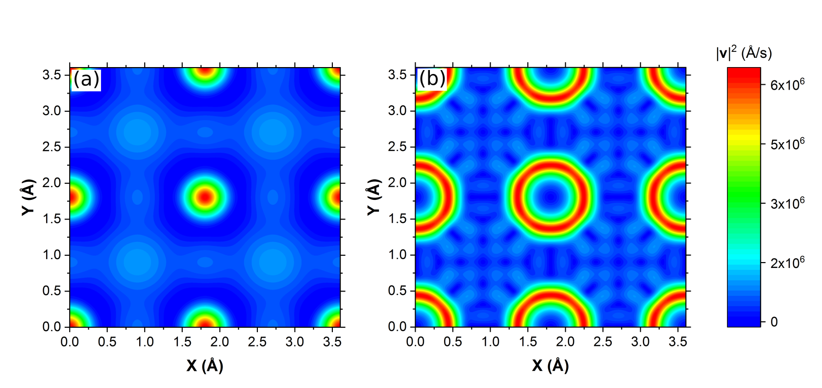
Figure 1: Exit wave function of Cu(100) zone axis orientation at 200keV and a thickness of 500 Å.

Simulations were performed at 200 keV and 30 keV. A variety of conditions were considered. Simulations were performed at normal incidence in the zone axis orientation of Cu(100), in the two beam condition for the 200 reflection, and in the case of a systematic row. Trajectories were propagated to a maximum thickness of 500 Å. In all cases, the incident wave function was chosen to be a plane wave.

III Results and discussion

III.1 Normal incidence

Simulations were first performed at normal incidence in the (100) zone axis orientation for copper. For an incident energy of 200 keV, $c_{s}=80$ and $c_{w}=90$ which resulted in a computation of 29 strong beams and 8 weak beams. Trajectories were first positioned equidistant from each other in a $10\times 10$ grid for an entire 3D analysis of the wave function progression. Then, to generate a 2D projection of the system, 50 trajectories along a line parallel to the $x$-axis in the center of the unit cell were initiated. Figure 2 (a) contains the 3D depiction of quantum trajectories passing through a 500 Å thick Cu crystal at 200 keV around the center atom column of the unit cell. Figure 2 (b) is a 2D projection on the $x-z$ plane under the same simulation conditions. Contrarily, for the afore mentioned figure, 50 trajectories were simulated along a line parallel to the $x$-axis, cross-sectioning the center of the unit cell. As a result, the behavior of these trajectories can be more clearly observed as they propagate through the material. Since the image represents a 2D projection, the patterns generated along the atom columns include oscillations coming out of the plane.

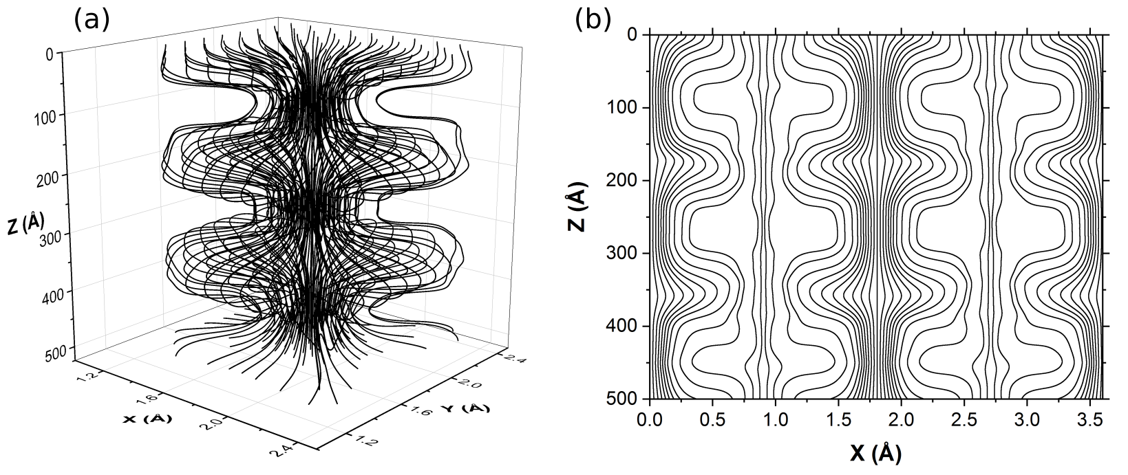
Figure 2: (a) 3D quantum trajectories at 200 keV of Cu(100) in zone axis orientation and (b) 2D projection on the $x-z$ plane of trajectories computed under the same imaging conditions but with 50 trajectories placed along a line.

As the trajectories propagate through the material, they are consistently attracted and repulsed by the atom columns. This effect is caused by the quantum force. Figure 3 shows the vector fields of the quantum and electrostatic forces acting around a single atom column.

Figure 3: (a) Quantum force generated by interaction between electron wave function and material around a single atom column and (b) electrostatic force of Cu.

If the only force acting on the propagating electrons was the electrostatic force generated by the material, then the particles would be strongly attracted towards the nucleus and would collapse without further transport. However, the total force exerted on the particles is the sum of the electrostatic force and the quantum force described by the hydrodynamic theory Chattaraj (2010). The quantum force, as seen in Figure 3 (a), contributes the repulsive force acting upon the trajectories which pushes the electrons to channel between and through the atom columns. The electrons are pulled towards the nucleus by both the quantum and electrostatic forces until a critical radius where the repulsive quantum force takes over and ensures that the particles do not collapse but continue to propagate through. The electrostatic force is on the order of 500 N while that of the quantum force is 1600 N showing that the magnitude of the quantum force supersedes that of the electrostatic, and this is evident by the path the electron trajectories take. This also demonstrates the quantum force’s role in elastic scattering, where the magnitude and direction of a scattering event can be described in terms of the quantum force exerted on the particle. The explanation for these events through the hydrodynamic theory can be coupled with the conventional dynamic theory to provide a more complete explanation of electron-matter interactions during transmission in an electron microscope.

Simulations were also performed at 30 keV to replicate wave function propagation in the energy range of a scanning electron microscope (SEM). Here, 57 strong beams and 20 weak beams were used in the computation. Figure 4 shows the 3D representation of the trajectories around a single atom column and the 2D projection across the entire unit cell.

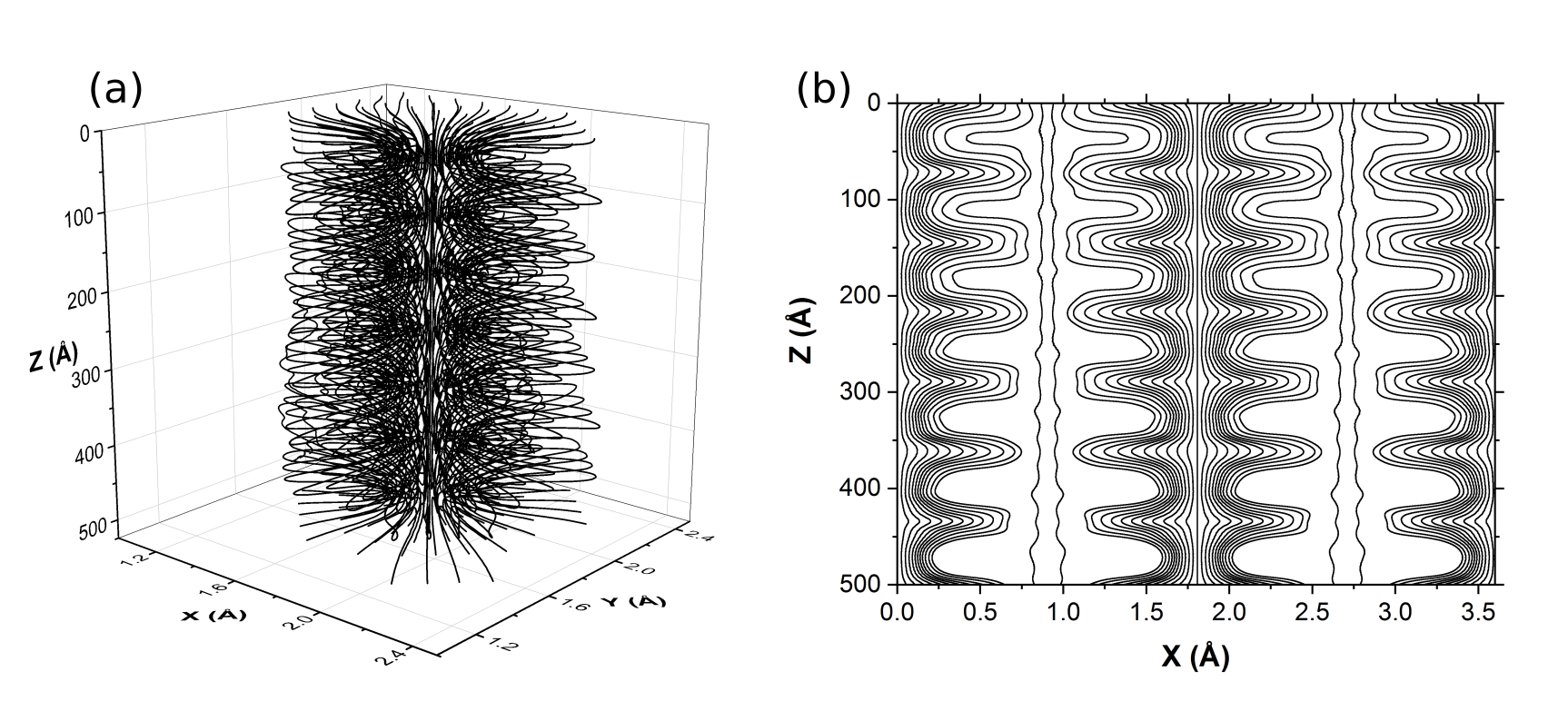
Figure 4: Simulations of a 30 keV electron beam incident on Cu(100) zone axis, (a) 3D representation of trajectories around a single atom column and (b) the 2D projection with 50 trajectories positioned on a line parallel to the $x$-axis.

Here, because the electron energy is significantly lower, there are many more scattering events that will occur causing more modulations of the wave function as it travels through the material. At a foil thickness of 500 Å, 30 keV is still large enough where the entire beam is transmitted through the film. The wave function however undergoes significantly more coherent scattering which is seen by the modulations in the trajectories. A consistency does get reached after a few hundreds of angstrom where there is less dispersion between the atom columns and the wave function becomes more confined to the sinusoidal displacements and group channeling around the atom columns. The higher frequency oscillations is again due to the action of the quantum force and this is seen in the velocity field of the wave function. Figure 5 shows the magnitude of the velocity field across the entire unit cell and its associated exit wave function.

Figure 5: (a) Intensity of exit wave function and (b) associated velocity field with color scale for simulation done at 30 keV in Cu(100) zone axis orientation.

While the intensity of the exit wave function is greatest at the atom columns, the velocity field shows that the particles’ radial velocity increases near the contours of the atom columns. The direction of the velocity is away from the columns indicating again the channeling effect. The quantum force at 30 keV is, in contrast, much more chaotic due to high potential for interactions and scattering at lower electron energies. Figure 6 shows the quantum force around an atom column at 30 keV.

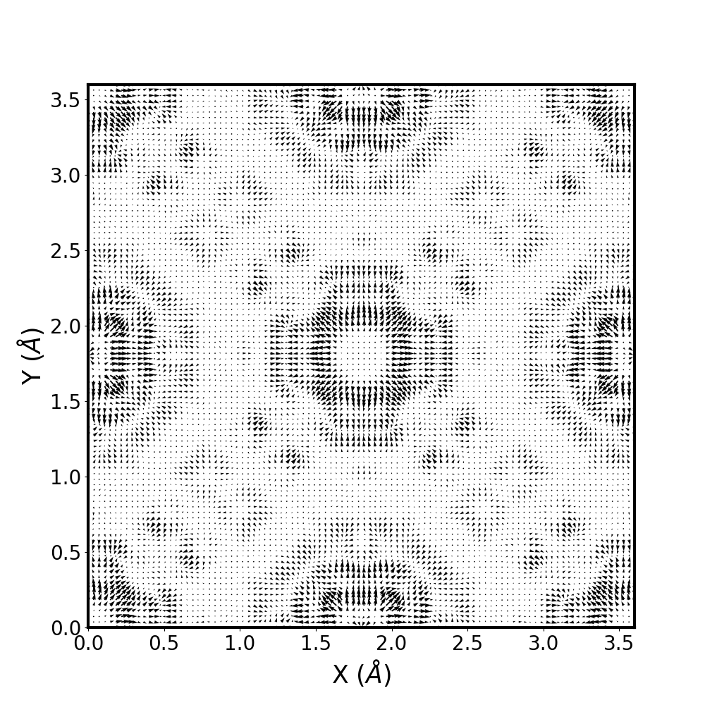
Figure 6: Quantum force at 30 keV across entire unit cell.

III.2 Two beam condition

Trajectories in the two beam approximation were simulated to display the particle paths under ideal diffraction conditions. Here, only two beams were considered in the Bloch wave calculation, $\mathbf{g}_{000}$ and $\mathbf{g}_{200}$. Simulations were again performed at 200 keV and 30 keV. As is the convention, a transverse component whose magnitude is equivalent to a tilt to the Bragg angle is added to the incident wave vector, instead of tilting the specimen itself. The transverse component added to the incident wave vector before normalization to the electron wave length was $|\mathbf{k}_{t}|=0.2766$ Å^-1. This ensured that the exact Bragg condition was met for $\mathbf{g}_{200}$. The associated quantum trajectories are displayed in Figure 7.

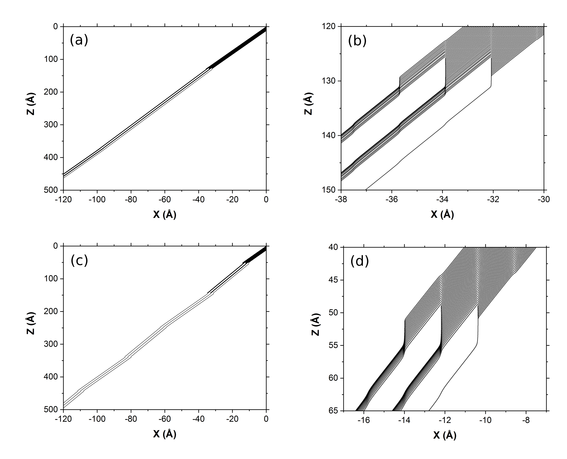
Figure 7: Quantum trajectories in the two beam condition for $\mathbf{g}=(200)$ for Cu at electron energies of (a) 200 keV and (c) 30 keV. A zoom in of the full simulated trajectories at a thickness at which the trajectories are separated for (b) 200 keV and (d) 30 keV is also displayed.

In the two beam condition, only the primary and diffracted beam contribute to the final wave function. Here, diffraction of the plane wave by the crystal causes the trajectories to be separated into what are the primary and diffracted beams. These trajectories then propagate accordingly resulting in the pattern that would be detected at the diffraction plane. Figures 7(a) and (c) display the entire propagation where once the plane wave diffracts, the coupled groups of trajectories continue as such. Figure 7(b) and (d) show a close up to the thickness where the trajectories originally separate showing exactly how the wave function is diffracted in the two beam condition. The small ripples in the grouped trajectories could be effects of the ”beating” caused by the two types of Bloch waves which have been previously related to the appearance of thickness fringes Egerton (2013). An important stipulation of the theory behind the quantum trajectory method is that the trajectories may not cross paths at a specified moment in time Pladevall and Mompart (2012). Therefore, there cannot be crossing from one beam to another in configuration space. However, the contributions of the two components of the travelling function do oscillate accordingly. Figure 8 shows the intensity of both waves $\psi_{\mathbf{0}}$ and $\psi_{\mathbf{g}}$ as a function of distance for the electron energies considered here.

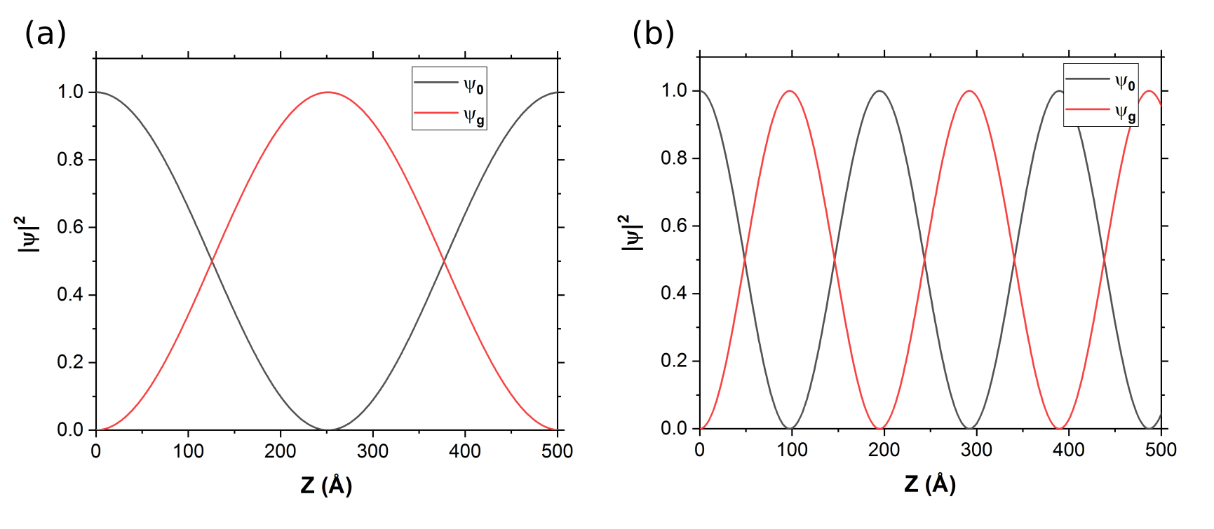
Figure 8: Beam intensity as a function of thickness for the $\mathbf{g}_{200}$ two beam condition at electron energies of (a) 200 keV and (b) 30 keV.

In accordance with diffraction theory, because the incident wave is tilted to exactly the Bragg condition and absorption is neglected, the intensities of each contributing beam oscillate continuously and the full intensity is completely transferred from one to the other Cowley (1995); Reimer and Kohl (2008). The extinction distance, $\xi_{\mathbf{g}}$, of a beam $\mathbf{g}$ is computed as De Graef (2003); Wang (1995),

$$\frac{1}{\xi_{\mathbf{g}}}=\frac{|U_{\mathbf{g}}|}{|\mathbf{k}_{0}+\mathbf{g}|\cos\alpha}$$ (12)

where $\alpha$ is the angle between $\mathbf{k}_{0}+\mathbf{g}$ and the surface normal of the material. For Cu, computed using the scattering factors obtained by Kirkland Kirkland (2010), $\xi_{\mathbf{200}}$ is 431.1 and 166.9 Å for 200 keV and 30 keV respectively. The wave lengths of the sinusoidal functions governing the intensities of both beams in Figure 8 correspond exactly to their respective extinction distances. This demonstrates the so called pendellösung Hagemann and Reimer (1979). The total wave function in real space is however continuous which is portrayed through the propagation of trajectories. When the incident beam is tilted outside of the Bragg condition, the structure is lost and the trajectories behave in a different way. Figure 9 shows trajectories computed from the same two beams but at normal incidence to the sample surface.

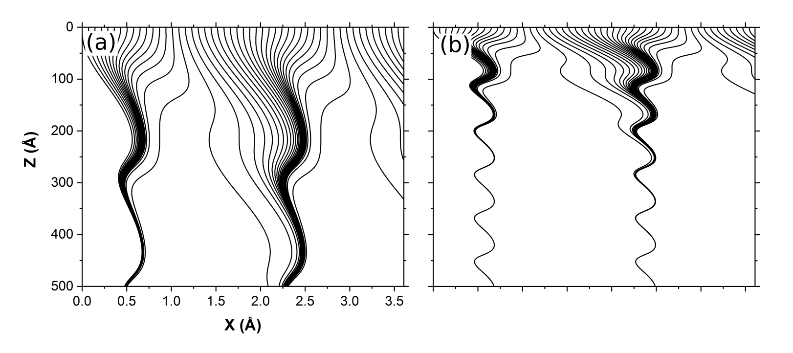
Figure 9: Quantum trajectories computed from two beams, $\psi_{\mathbf{0}}$ and $\psi_{\mathbf{g}}$, where $\mathbf{g}=(200)$. Propagation is at normal incidence and the electron energies are (a) 200 keV and (b) 30 keV respectively.

Here, both the primary beam $\psi_{\mathbf{0}}$ and $\psi_{\mathbf{g}}$ are the sole beams used in the computation. Because the Bragg condition is not satisfied, the beam is not diffracted and instead oscillations similar to those seen in the zone axis orientation are apparent. This indicates that outside the Bragg condition, if only two beams contribute to the Bloch wave expression, the wave function is only incoherently scattered by the atom columns. Evaluating the problem from a hydrodynamic approach can aid in explaining the two beam diffraction process in real space with the evolution of the wave function.

III.3 Systematic row

The special condition of the systematic row is important for convergent beam electron diffraction (CBED) patterns, simulations of bend contours, and defect analysis Phillips et al. (2011); Rez et al. (1977); De Graef (2003). When multiples of a beam $\mathbf{g}$ are excited, a material is said to be in a systematic row orientation De Graef (2003). Contrasts such as those found in bend contours are generated by the excitation of higher orders of a single beam where multiple such reflections are in the Bragg condition De Graef (2003). In CBED imaging, the contrasts within a single spot present themselves as bands. This is simulated by including only multiples of a single beam direction in the dynamic calculation De Graef (2003). If the simulation is done over increments of the transverse wave component such that $\mathbf{k}_{t}/\mathbf{g}$ is incremented uniformly, then rocking curves may be generated Reimer and Kohl (2008). The interest here is of the interaction of the traveling particles through a material when they are diffracted in such a condition. The $\mathbf{g}=(100)$ systematic row was simulated at normal incidence where 7 beams were considered, from $-3\mathbf{g}$ to $3\mathbf{g}$. Figure 10 displays trajectories obtained at both 200 keV and 30 keV.

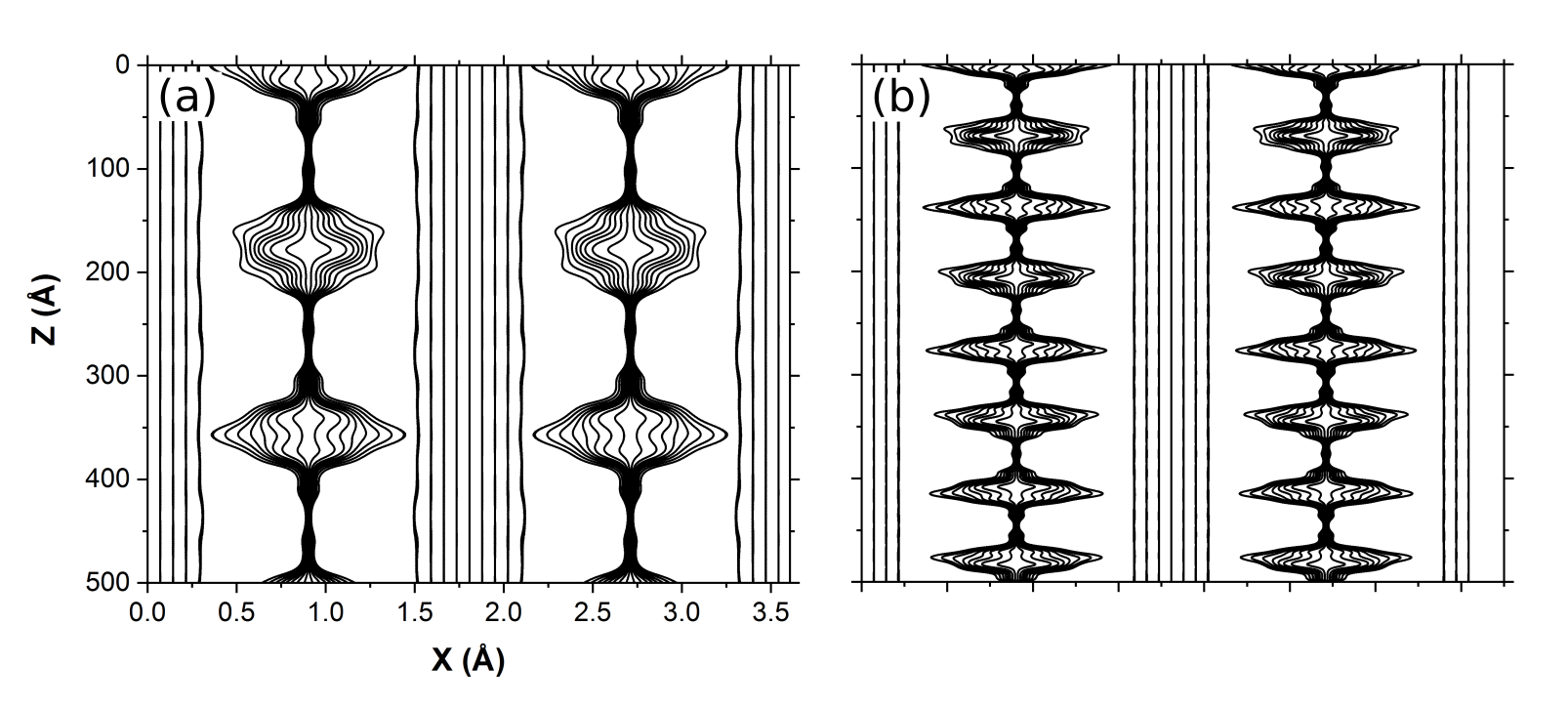
Figure 10: Trajectories propagated in the $\mathbf{g}=(100)$ systematic row condition with $k_{t}=0$ at electron energies of (a) 200 keV and (b) 30 keV.

The trajectories along the atom columns are propagated straight through with little deviation while those between the atom columns deviate towards the columns and back towards their center, replicating a similar case to that of normal incidence. Again, initial positions were chosen in a systematic way to map out the entire beam. In reality, the uncertainty of the initial position would dictate whether the electron remains in the band or deviates between them. The exit wave function and quantum potential of the simulation performed at 200 keV are displayed in Figure 11. The differences in intensities from the center of the bands outwards are caused by the contributions of electrons passing between the columns. This is due to the effects of the quantum potential seen in Figure 11 (b). The quantum potential is positive exactly in the center of the bands visible in the exit wave function and decreases to a sink as it approaches them. This creates a force that is constantly deviated to and from the contract bands, creating the trajectory paths of Figure 10.

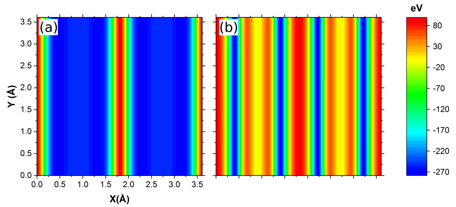
Figure 11: (a) Intensity distribution of exit wave function at 500 Å in the $\mathbf{g}=(100)$ systematic row orientation and (b) the corresponding quantum potential.

The paths taken by the trajectories demonstrate the dynamic effects that would not otherwise be generated using a kinematic theory and provide an explanation for differences in contrast across such imaging conditions.

IV Conclusions

The quantum trajectory method was coupled with a Bloch wave calculation of the transmitted wave function of an electron beam through a thin copper foil. Simulations were performed in the zone axis case, the two beam condition and the systematic row condition. It was shown that quantum trajectories can provide useful insight into electron-matter interactions by displaying where the particles may pass as they are transmitted through an imaged material. In the zone axis orientation, it is shown that the electrons are channeled by the constant attractive and repulsive force exerted by the quantum potential that surrounds the atom columns. In the two beam condition, diffraction of the plane wave occurred by the quick separation of trajectories in to groups corresponding to the diffracted and primary beams. Verifications of the two beam calculations were made through mapping of the intensities of each the primary beam and the diffracted one, where the contributions of each were shown to oscillate continuously. Finally, in the case of the systematic row, the contrast around the bands was explained by oscillations in the quantum trajectories between atom columns. In total, the method of associating trajectories to the propagating wave function was shown to describe particle scattering with the involvement of quantum effects and can be coupled in the future to Monte Carlo techniques to create all encompassing image and particle simulations in electron microscopy.

References

- Kirkland (2010) J. Kirkland, Advanced Computing in Electron Microscopy (Springer US, 2010).
- Allen et al. (2015) L. Allen, A. D’Alfonso, and S. Findlay, Ultramicroscopy 151, 11 (2015), special Issue: 80th Birthday of Harald Rose; {PICO} 2015 Third Conference on Frontiers of Aberration Corrected Electron Microscopy.
- den Broek et al. (2015) W. V. den Broek, X. Jiang, and C. Koch, Ultramicroscopy 158, 89 (2015).
- Dwyer (2010) C. Dwyer, Ultramicroscopy 110, 195 (2010).
- Pennycook and Jesson (1990) S. J. Pennycook and D. E. Jesson, Phys. Rev. Lett. 64, 938 (1990).
- Winkelmann et al. (2007) A. Winkelmann, C. Trager-Cowan, F. Sweeney, A. P. Day, and P. Parbrook, Ultramicroscopy 107, 414 (2007).
- Findlay et al. (2003) S. Findlay, L. Allen, M. Oxley, and C. Rossouw, Ultramicroscopy 96, 65 (2003).
- Rossouw et al. (2003) C. Rossouw, L. Allen, S. Findlay, and M. Oxley, Ultramicroscopy 96, 299 (2003), proceedings of the International Workshop on Strategies and Advances in Atomic Level Spectroscopy and Analysis.
- Gauvin et al. (2006) R. Gauvin, E. Lifshin, H. Demers, P. Horny, and H. Campbell, Microscopy and Microanalysis 12, 49 (2006).
- Salvat (2015) F. Salvat, Annals of Nuclear Energy 82, 98 (2015).
- Trahan and Wyatt (2006) C. Trahan and R. Wyatt, Quantum Dynamics with Trajectories: Introduction to Quantum Hydrodynamics, Interdisciplinary Applied Mathematics (Springer, 2006).
- Oriols (2007) X. Oriols, Phys. Rev. Lett. 98, 066803 (2007).
- Sanz and Miret-Artés (2012) Á. Sanz and S. Miret-Artés, A Trajectory Description of Quantum Processes. I. Fundamentals: A Bohmian Perspective, Lecture Notes in Physics (Springer Berlin Heidelberg, 2012).
- Sanz et al. (2010) A. Sanz, M. Davidović, M. Božić, and S. Miret-Artés, Annals of Physics 325, 763 (2010).
- Sanz et al. (2002) A. S. Sanz, F. Borondo, and S. Miret-Artés, Journal of Physics: Condensed Matter 14, 6109 (2002).
- Efthymiopoulos et al. (2012) C. Efthymiopoulos, N. Delis, and G. Contopoulos, Annals of Physics 327, 438 (2012).
- Rudinsky et al. (2017) S. Rudinsky, A. S. Sanz, and R. Gauvin, Journal of Chemical Physics 146, 104702 (2017).
- Zhang et al. (2015) M. Zhang, Y. MING, R. ZENG, and Z. DING, Journal of Microscopy 260, 200 (2015).
- Zeng and Ding (2011) R. Zeng and Z. Ding, Journal of Surface Analysis 17, 198 (2011).
- Picard et al. (2014) Y. Picard, M. Liu, J. Lammatao, R. Kamaladasa, and M. D. Graef, Ultramicroscopy 146, 71 (2014).
- Cheng et al. (2018) L. Cheng, Y. Ming, and Z. J. Ding, New Journal of Physics 20, 113004 (2018).
- De Graef (2003) M. De Graef, Introduction to Conventional Transmission Electron Microscopy (Cambridge University Press, 2003).
- Zuo and Weickenmeier (1995) J. Zuo and A. Weickenmeier, Ultramicroscopy 57, 375 (1995).
- Wang and Graef (2016) A. Wang and M. D. Graef, Ultramicroscopy 160, 35 (2016).
- Sanz and Miret-Artés (2013) Á. Sanz and S. Miret-Artés, A Trajectory Description of Quantum Processes. II. Applications: A Bohmian Perspective, Lecture Notes in Physics (Springer Berlin Heidelberg, 2013).
- Chattaraj (2010) P. Chattaraj, Quantum Trajectories, Atoms, Molecules, and Clusters (CRC Press, 2010).
- Egerton (2013) R. Egerton, Electron Energy-Loss Spectroscopy in the Electron Microscope (Springer US, 2013).
- Pladevall and Mompart (2012) X. Pladevall and J. Mompart, Applied Bohmian Mechanics: From Nanoscale Systems to Cosmology (Pan Stanford, 2012).
- Cowley (1995) J. Cowley, Diffraction Physics, North-Holland Personal Library (Elsevier Science, 1995).
- Reimer and Kohl (2008) L. Reimer and H. Kohl, Transmission Electron Microscopy: Physics of Image Formation, Springer Series in Optical Sciences (Springer, 2008).
- Wang (1995) Z. Wang, Elastic and inelastic scattering in electron diffraction and imaging, Language of science (Plenum Press, 1995).
- Hagemann and Reimer (1979) P. Hagemann and L. Reimer, Philosophical Magazine A 40, 367 (1979), http://dx.doi.org/10.1080/01418617908234846 .
- Phillips et al. (2011) P. Phillips, M. Mills, and M. D. Graef, Philosophical Magazine 91, 2081 (2011), https://doi.org/10.1080/14786435.2010.547526 .
- Rez et al. (1977) P. Rez, C. J. Humphreys, and M. J. Whelan, The Philosophical Magazine: A Journal of Theoretical Experimental and Applied Physics 35, 81 (1977), https://doi.org/10.1080/14786437708235974 .