BCOR5mm DIVclassic headincludefalse footincludefalse pagesizeauto headingssmall numbersendperiod plainheaderbreak Definition]Problem Definition]Assumption Definition]Theorem Definition]Proposition Definition]Lemma Definition]Corollary Definition]Algorithm  
Tensor-Free Proximal Methods for Lifted Bilinear/Quadratic Inverse Problems with Applications to Phase Retrieval
Robert Beinert¹ and Kristian Bredies^1
1 Institut für Mathematik und Wissenschaftliches Rechnen Karl-Franzens-Universität Graz Heinrichstraße 36 8010 Graz, Austria
Correspondence
R. Beinert:
K. Bredies:
 
             Abstract.   We propose and study a class of novel algorithms that aim at solving bilinear and quadratic inverse problems. Using a convex relaxation based on tensorial lifting, and applying first-order proximal algorithms, these problems could be solved numerically by singular value thresholding methods. However, a direct realization of these algorithms for, e.g., image recovery problems is often impracticable, since computations have to be performed on the tensor-product space, whose dimension is usually tremendous. To overcome this limitation, we derive tensor-free versions of common singular value thresholding methods by exploiting low-rank representations and incorporating an augmented Lanczos process. Using a novel reweighting technique, we further improve the convergence behavior and rank evolution of the iterative algorithms. Applying the method to the two-dimensional masked Fourier phase retrieval problem, we obtain an efficient recovery method. Moreover, the tensor-free algorithms are flexible enough to incorporate a-priori smoothness constraints that greatly improve the recovery results.
             Keywords.  Tensor-free proximal methods, tensorial lifting, nuclear norm relaxation, reweighting techniques, bilinear inverse problem, quadratic inverse problem, masked Fourier phase retrieval
             AMS subject classification.  45Q05, 65F10, 65R32, 65K10
 

1 Introduction

The theory of inverse problems is nowadays one of the main tools to deal with recovery problems in medicine, engineering, and life sciences. The real-world applications of this theory embrace for instance computed tomography, magnetic resonance imaging, and deconvolution problems in microscopy, see [BB98, MS12, Ram05, SW13, Uhl03, Uhl13]. Besides these recent monographs, which are only a small selection, there exist many further publications about applications, regularization, and numerical solvers.

In this paper, we consider the subclass of bilinear and quadratic inverse problems [BB18]. Problem formulations of these kinds originate form real-world applications in imaging and physics [SGG⁺09] like blind deconvolution [BS01, JR06], deautoconvolution [GH94, GHB⁺14, ABHS16], phase retrieval [DF87, Mil90, SSD⁺06], parallel imaging in MRI [BBM⁺04], and parameter identification in EIT [MS12]. Although these problems may be seen as non-linear inverse problems and can be solved by appropriate non-linear solvers, the question arises if we can exploit the specific bilinear or quadratic structure of these problem.

One of the most famous approaches of this kind is PhaseLift [CSV13], where the generic phase retrieval problem is lifted to a linear inverse problem with rank-one constraint using the universal property of the tensor product. After a relaxation the lifted problem is solved by semi-definite programming. From the theoretical side, one has proved that this methodology yields the true solution with very high probability. Based on PhaseLift, we will derive convex lifting methods for general bilinear and quadratic inverse problems.

Similarly to PhaseLift, the relaxations here require the minimization of a nuclear norm functional on the tensor product, which can be done by applying proximal minimization methods, see for instance [CP16] and references therein. Since the dimension of the lifted problem can become huge, the question arises how one can implement these methods numerically. Therefore, we develop tensor-free, equivalent versions that can be performed in an efficient and memory-saving manner. The main benefit is here that the tensor-free reformulations of the required tensorial operations are performed exactly without additional error. To improve the convergence and solution behaviour, we additionally propose a novel reweighting technique

The paper is organized as follows: In Section 2, we introduce the considered bilinear and quadratic inverse problems in more detail. The focus here lies on the bilinear setting since quadratic formulations are based on underlying bilinear structures. Based on the universal property of bilinear mappings and the nuclear norm heuristic, we then derive a relaxed convex minimization problem with linear lifted forward operator. To stabilize the lifted problem regarding noise and measurement errors, we additionally consider a Tikhonov approach.

In Section 3, we develop a proximal solver based on the first-order primal-dual method of Chambolle and Pock [CP11] to solve the lifted problem numerically. The primal-dual iteration is here only one explicit example and can be replaced by any other proximal method. In so doing, we obtain a singular value thresholding depending on the actual Hilbert spaces building the domain of the original problem. Although the tensorial lifting allows us to apply linear methods, the dimension of the relaxed minimization problem becomes tremendous.

To overcome this issue, we derive a tensor-free representation of the suggested algorithm. The efficient computation of the required singular value thresholding is here ensured by exploiting an orthogonal power iteration or, alternatively, an augmented Lanczos process, see Section 4. Moreover, in Section 5, we introduce a novel Hilbert space reweighting to promote low-rank iterations and solutions. We complete the paper with a numerical study, where we consider the masked Fourier phase retrieval, see Section 6.

The contribution of the paper is twofold: Firstly, we derive a novel tensor-free proximal algorithm based on a convex lifting and relaxation. Secondly, we introduce a novel phase retrieval technique, which solves high-dimensional instances of the masked phase retrieval problem. Moreover, our approach allows us to incorporate smoothness constraints or relation between different pixels to improve the convergence of the algorithm.

2 Convex liftings of bilinear and quadratic inverse problems

Bilinear and quadratic problem formulations arise in a wide range of applications in imaging and physics [SGG⁺09] like blind deconvolution [BS01, JR06], deautoconvolution [GH94, GHB⁺14, ABHS16], phase retrieval [DF87, Mil90, SSD⁺06], parallel imaging in MRI [BBM⁺04], and parameter identification in EIT [MS12]. Since we are mainly interested in computing a numerical solution, we restrict ourselves to finite-dimensional bilinear problems of the form

$$\mathcal{B}(\bm{u},\bm{v})=\bm{g}^{\dagger},\vspace*{5pt} \mathfrak{B}$$ ()

where $\mathcal{B}$ is a bilinear operator from $\mathcal{H}_{1}\times\mathcal{H}_{2}$ into $\mathcal{K}$, and where $\mathcal{H}_{1}\simeq\mathbb{R}^{N_{1}}$, $\mathcal{H}_{2}\simeq\mathbb{R}^{N_{2}}$, and $\mathcal{K}\simeq\mathbb{R}^{M}$ are real finite-dimensional Hilbert spaces equipped with some inner product. Simultaneously, we study finite-dimensional quadratic problems of the form

$$\mathcal{Q}(\bm{u})=\bm{g}^{\dagger}. \mathfrak{Q}$$ ()

A quadratic operator $\mathcal{Q}\colon\mathcal{H}\to\mathcal{K}$ is here the restriction of an associate bilinear operator $\mathcal{B}_{\mathcal{Q}}:\mathcal{H}\times\mathcal{H}\to\mathcal{K}$ to its diagonal and is thus given by $\mathcal{Q}(\bm{u})\coloneqq\mathcal{B}_{\mathcal{Q}}(\bm{u},\bm{u})$. Again, the Hilbert spaces $\mathcal{H}$ and $\mathcal{K}$ are finite dimensional. Without loss of generality, one may assume that the associated bilinear operator is symmetric, i.e. $\mathcal{B}_{\mathcal{Q}}(\bm{u},\bm{v})=\mathcal{B}_{\mathcal{Q}}(\bm{v},\bm{u})$ for all $\bm{u}$, $\bm{v}\in\mathcal{H}$, which can be enforced by considering $\nicefrac{{1}}{{2}}\,\mathcal{B}_{\mathcal{Q}}(\bm{u},\bm{v})+\nicefrac{{1}}{{2}}\,\mathcal{B}_{\mathcal{Q}}(\bm{v},\bm{u})$. However, we will make no use of this restriction.

For the sake of simplicity, we use the following notation and write an arbitrary vector $\bm{u}\in\mathcal{H}_{1}$ in the form $\bm{u}\coloneqq(u_{n})_{n=0}^{N_{1}-1}\in\mathbb{R}^{N_{1}}$, which may be interpreted as the coefficient vector with respect to some finite basis. The inner product of $\mathcal{H}_{1}$ can now be stated in the form $\langle\cdot,\cdot\rangle_{\mathcal{H}_{1}}\coloneqq\langle\bm{H}_{1}\,\cdot,\cdot\rangle=\langle\cdot,\bm{H}_{1}\,\cdot\rangle$, where $\bm{H}_{1}$ is some symmetric, positive definite matrix in $\mathbb{R}^{N_{1}\times N_{1}}$, and where the inner products on the right-hand side denote the usual Euclidian inner product $\left\langle\bm{u},\bm{v}\right\rangle\coloneqq\bm{v}^{*}\bm{u}$. Here $\cdot^{*}$ labels the transposition of a vector or matrix. For the remaining spaces $\mathcal{H}_{2}$ and $\mathcal{K}$, we proceed in the same manner with the associate matrices $\bm{H}_{2}\in\mathbb{R}^{N_{2}\times N_{2}}$ and $\bm{K}\in\mathbb{R}^{M\times M}$, respectively.

Although we restrict ourselves to the real-valued setting, all following algorithms and statements remain valid for the complex-valued setting, where one considers sesquilinear mappings $\mathcal{B}\colon\mathcal{H}_{1}\times\mathcal{H}_{2}\to\mathcal{K}$ with $\mathcal{H}_{1}\simeq\mathbb{C}^{N_{1}}$, $\mathcal{H}_{2}\simeq\mathbb{C}^{N_{2}}$, and $\mathcal{K}\simeq\mathbb{C}^{M}$. Changing the notation to $\bm{u}\coloneqq(u_{n})_{n=0}^{N_{1}-1}\in\mathbb{C}^{N_{1}}$, replacing the property ‘symmetric’ by ‘Hermitian,’ and using the real part of the inner products, e.g. $\left\langle\bm{u},\bm{v}\right\rangle=\Re[\bm{v}^{*}\bm{u}]$, where $\cdot^{*}$ is the transposition and conjugation, all considerations translate one to one. In the complex case, the associate matrices $\bm{H}_{1}$, $\bm{H}_{2}$, and $\bm{K}$ may also be complex-valued, Hermitian, and positive definite.

Inspired by PhaseLift [CESV13, CSV13], which exploits the solution strategy developed for matrix completion problems [CCS10, MGC11], we suggest to tackle the general bilinear and quadratic inverse problem ($\mathfrak{B}$) and ($\mathfrak{Q}$) by convex liftings and relaxations. Our approach is here based on the so-called universal property of the tensor product with respect to bilinear mappings, see for instance [Rya02, Theorem 2.9]. In the finite-dimensional setting, the lifting may be stated as follows.

[Bilinear lifting, [Rya02]] For every bilinear mapping $\mathcal{B}\colon\mathcal{H}_{1}\times\mathcal{H}_{2}\rightarrow\mathcal{K}$, there exists a unique linear mapping $\breve{\mathcal{B}}\colon\mathcal{H}_{1}\otimes\mathcal{H}_{2}\rightarrow\mathcal{K}$ such that $\breve{\mathcal{B}}(\bm{u}\otimes\bm{v})=\mathcal{B}(\bm{u},\bm{v})$.

In the finite-dimensional setting considered by us, the tensor product $\mathcal{H}_{1}\otimes\mathcal{H}_{2}$ can be simply identified with the matrix space $\mathbb{R}^{N_{2}\times N_{1}}$, where the rank-one tensor $\bm{u}\otimes\bm{v}$ corresponds to the matrix $\bm{v}\bm{u}^{*}=(v_{n_{2}}u_{n_{1}})_{n_{2}=0,n_{1}=0}^{N_{2}-1,N_{1}-1}$. The universal property is also applicable to quadratic mappings, where the tensor product $\mathcal{H}\otimes\mathcal{H}$ is restricted to the subspace of symmetric tensors $\mathcal{H}\otimes_{\mathrm{sym}}\mathcal{H}$ which is isomorphic to the space of symmetric matrices.

[Quadratic lifting] For every bounded quadratic mapping $\mathcal{Q}\colon\mathcal{H}\times\rightarrow\mathcal{K}$, there exists a unique linear mapping $\breve{\mathcal{Q}}\colon\mathcal{H}\otimes_{\mathrm{sym}}\mathcal{H}\rightarrow\mathcal{K}$ such that $\breve{\mathcal{Q}}(\bm{u}\otimes\bm{u})=\mathcal{Q}(\bm{u})$.

Proof 1.

Since the lifting $\breve{\mathcal{B}}$ of the associate bilinear mapping $\mathcal{B}$ is unique, the restriction $\breve{\mathcal{Q}}\coloneqq\breve{\mathcal{B}}|_{\mathcal{H}\otimes_{\mathrm{sym}}\mathcal{H}}$ yields a unique linear mapping with the asserted properties.

Due to the uniqueness of the lifting, the bilinear inverse problem ($\mathfrak{B}$) and the quadratic inverse problem ($\mathfrak{Q}$) are equivalent to the linear inverse problems

$$\breve{\mathcal{B}}(\bm{w})=\bm{g}^{\dagger} \qquad\text{subject to}\qquad\operatorname{rank}(\bm{w})\leq 1 \breve{\mathfrak{B}}$$ ()

and

$$\breve{\mathcal{Q}}(\bm{w})=\bm{g}^{\dagger} \qquad\text{subject to}\qquad\operatorname{rank}(\bm{w})\leq 1,\quad\bm{w}\succeq\bm{0}, \breve{\mathfrak{Q}}$$ ()

where the additional constraint $\bm{w}\succeq\bm{0}$ means that $\bm{w}$ is positive semi-definite. Although the positive semi-definiteness of the lifted quadratic problem is not mandatory, it strongly reduces the space of possible solutions. The central benefit of these reformulations is the shift of the non-linearity of the forward operator into the rank-one constraint. Although the problem is now linear, we have to deal with an additional non-convex side condition.

In order to eliminate the non-linear constraint for bilinear operators, we first rewrite ($\breve{\mathfrak{B}}$) into the rank minimization problem

$$\operatorname*{minimize}\quad\operatorname{rank}(\bm{w})\quad\text{with}\quad\breve{\mathcal{B}}(\bm{w})=\bm{g}^{\dagger}$$

and then relax the non-convex objective function by replacing it with the nuclear or projective norm $||\hskip 1.0pt\cdot\hskip 1.0pt||_{\mathcal{H}_{1}\otimes_{\uppi}\mathcal{H}_{2}}$ of the tensor $\bm{w}$. Depending on the Hilbert spaces $\mathcal{H}_{1}$ and $\mathcal{H}_{2}$, this norm is defined by

$$||\hskip 1.0pt\bm{w}\hskip 1.0pt||_{\mathcal{H}_{1}\otimes_{\uppi}\mathcal{H}_{2}}\coloneqq\inf\biggl{\{}\sum_{n=1}^{N}||\hskip 1.0pt\bm{u}_{n}\hskip 1.0pt||_{\mathcal{H}_{1}}\,||\hskip 1.0pt\bm{v}_{n}\hskip 1.0pt||_{\mathcal{H}_{2}}:\bm{w}=\sum_{n=1}^{N}\bm{u}_{n}\otimes\bm{v}_{n},N\in\mathbb{N}\biggr{\}},$$

where the infimum is taken over all finite representations of the tensor $\bm{w}$. In so doing, we finally obtain the convex minimization problem

$$\operatorname*{minimize}\quad||\hskip 1.0pt\bm{w}\hskip 1.0pt||_{\mathcal{H}_{1}\otimes_{\uppi}\mathcal{H}_{2}}\quad\text{subject to}\quad\breve{\mathcal{B}}(\bm{w})=\bm{g}^{\dagger},\vspace*{5pt} \mathfrak{B}_{0}$$ ()

i.e., with linear constraints.

Since $\mathcal{H}_{1}$ as well as $\mathcal{H}_{2}$ is a Hilbert space, the nuclear norm here coincides with the trace class norm or with the Schatten one-norm; so the nuclear norm is simply the sum of the corresponding singular values of the matrix $\bm{w}\in\mathbb{R}^{N_{2}\times N_{1}}$ with respect to the Hilbert spaces $\mathcal{H}_{1}$ and $\mathcal{H}_{2}$, cf. for instance [Wer02, Satz VI.5.5].

[Projective norm, [Wer02]] For $\bm{w}\in\mathcal{H}_{1}\otimes\mathcal{H}_{2}$, the projective norm is given by $||\hskip 1.0pt\bm{w}\hskip 1.0pt||_{\mathcal{H}_{1}\otimes_{\uppi}\mathcal{H}_{2}}=\sum_{n=0}^{R-1}\sigma_{n}$, where $\sigma_{n}$ denotes the $n$-th singular value and $R$ the rank of $\bm{w}$.

The main idea behind the nuclear norm heuristic is that the projective norm is the convex envelope of the rank on the unit ball with respect to the spectral norm. Usually, the nuclear norm heuristic empirically yields low-rank solutions of the matrix equation $\breve{\mathcal{B}}(\bm{w})=\bm{g}^{\dagger}$, see for example [CCS10, MGC11, RFP10] and references therein. If the lifted operator $\breve{\mathcal{B}}$ fulfills an appropriate restricted isometry property, one can rigorously prove that the bilinear inverse problem ($\mathfrak{B}$) and the relaxed nuclear norm minimization problem ($\mathfrak{B}_{0}$) are equivalent, see [RFP10, Theorem 3.3].

For quadratic inverse problems, we follow a similar approach. This means that we first rewrite ($\mathfrak{Q}$) into a rank minimization problem over the positive semi-definite (symmetric) matrix cone. In order to obtain a convex minimization problem, we again replace the objective function by the projective norm. Since the singular values $\sigma_{n}$ of a symmetric tensor $\bm{w}$ coincide with the absolute value of its eigenvalues $\lambda_{n}$, the positive semi-definiteness may be incorporated into the projective norm by

$$||\hskip 1.0pt\bm{w}\hskip 1.0pt||_{\mathcal{H}\otimes_{\uppi}\mathcal{H}}^{+}\coloneqq\sum_{n=0}^{R-1}\lambda_{n}+\chi_{[0,\infty)}(\lambda_{n}),$$

where the indicator function $\chi_{[0,\infty)}$ is equal to $0$ for arguments in $[0,\infty)$ and $+\infty$ otherwise; so the modified projective “norm” $||\hskip 1.0pt\cdot\hskip 1.0pt||_{\mathcal{H}\otimes_{\uppi}\mathcal{H}}^{+}$ sums up the non-negative eigenvalues for positive semi-definite tensors and is infinity otherwise. To solve the quadratic inverse problem ($\mathfrak{Q}$) numerically, we thus consider the convex minimization problem

$$\operatorname*{minimize}\quad||\hskip 1.0pt\bm{w}\hskip 1.0pt||_{\mathcal{H}\otimes_{\uppi}\mathcal{H}}^{+}\quad\text{subject to}\quad\breve{\mathcal{Q}}(\bm{w})=\bm{g}^{\dagger}. \mathfrak{Q}_{0}$$ ()

Up to this point, the given data $\bm{g}^{\dagger}$ have been known exactly. A first approach to incorporate noisy measurements into the inverse problems ($\mathfrak{B}$) and ($\mathfrak{Q}$) could be to extend the subspace of exact solutions with respect to a supposed error level. More precisely, one may consider the minimization problems

$$\operatorname*{minimize}\quad||\hskip 1.0pt\bm{w}\hskip 1.0pt||_{\mathcal{H}_{1}\otimes_{\uppi}\mathcal{H}_{2}} \quad\text{subject to}\quad||\hskip 1.0pt\breve{\mathcal{B}}(\bm{w})-\bm{g}^{\epsilon}\hskip 1.0pt||_{\mathcal{K}}\leq\epsilon \mathfrak{B}_{\epsilon}$$ ()

and

$$\operatorname*{minimize}\quad||\hskip 1.0pt\bm{w}\hskip 1.0pt||_{\mathcal{H}\otimes_{\uppi}\mathcal{H}}^{+} \quad\text{subject to}\quad||\hskip 1.0pt\breve{\mathcal{Q}}(\bm{w})-\bm{g}^{\epsilon}\hskip 1.0pt||_{\mathcal{K}}\leq\epsilon. \mathfrak{Q}_{\epsilon}$$ ()

In other words, we minimize over all solutions that approximate the given noisy data $\bm{g}^{\epsilon}$ with $||\hskip 1.0pt\bm{g}-\bm{g}^{\epsilon}\hskip 1.0pt||_{\mathcal{K}}\leq\epsilon$ up to the error level $\epsilon$.

Another approach is to incorporate the data fidelity of the possible solutions directly into the objective function. Following this approach, we may minimize a Tikhonov functional with projective norm regularization to solve ($\mathfrak{B}$) and ($\mathfrak{Q}$). In more detail, we consider the problems

$$\operatorname*{minimize}\quad\tfrac{1}{2}\,||\hskip 1.0pt\breve{\mathcal{B}}(\bm{w})-\bm{g}^{\epsilon}\hskip 1.0pt||_{\mathcal{K}}^{2}+\alpha\,||\hskip 1.0pt\bm{w}\hskip 1.0pt||_{\mathcal{H}_{1}\otimes_{\uppi}\mathcal{H}_{2}} \mathfrak{B}_{\alpha}$$ ()

and

$$\operatorname*{minimize}\quad\tfrac{1}{2}\,||\hskip 1.0pt\breve{\mathcal{Q}}(\bm{w})-\bm{g}^{\epsilon}\hskip 1.0pt||_{\mathcal{K}}^{2}+\alpha\,||\hskip 1.0pt\bm{w}\hskip 1.0pt||^{+}_{\mathcal{H}\otimes_{\uppi}\mathcal{H}}. \mathfrak{Q}_{\alpha}$$ ()

All proposed convex relaxations of the lifted problems ($\breve{\mathfrak{B}}$) and ($\breve{\mathfrak{Q}}$) have in common that the minimization of the projective norm usually promotes low-rank tensors and, in the best case, yields a rank-one solutions. The later case forms our basic premise to derive numerical solutions.

[Basic premise] Suppose that the solutions $\bm{w}$ of the relaxation ($\mathfrak{B}_{0}$), ($\mathfrak{B}_{\epsilon}$), or ($\mathfrak{B}_{\alpha}$) are at most rank-one tensors $\bm{u}\otimes\bm{v}$ such that $(\bm{u},\bm{v})$ (approximately) solves the bilinear inverse problem ($\mathfrak{B}$). Likewise, suppose that the solutions $\bm{w}$ of the relaxations ($\mathfrak{Q}_{0}$), ($\mathfrak{Q}_{\epsilon}$), or ($\mathfrak{Q}_{\alpha}$) have at most rank one so that they (approximately) solve the quadratic inverse problem ($\mathfrak{Q}$).

3 Proximal algorithms for the lifted problem

To exploit the nuclear norm heuristic, we have to solve the minimization problem ($\mathfrak{B}_{0}$), ($\mathfrak{B}_{\epsilon}$), ($\mathfrak{B}_{\alpha}$), ($\mathfrak{Q}_{0}$), ($\mathfrak{Q}_{\epsilon}$), and ($\mathfrak{Q}_{\alpha}$) in an efficient manner. Looking back at the comprehensive literature about matrix completion [CR09, CCS10, MGC11], low-rank solutions of matrix equations [RFP10], and PhaseLift [CESV13, CSV13], there exists several numerical methods like interior-point methods for semi-definite programming, fixed point iterations, singular value thresholding algorithm, projected subgradient methods, and low-rank parametrization approaches.

In order to solve the lifted bilinear and quadratic inverse problems, we follow another approach. Let us first consider the actual structure of the six derived minimization problems in Section 2, which is given by

$$\operatorname*{minimize}\quad F(\mathcal{A}(\bm{w}))+G(\bm{w}),$$ (1)

where $\mathcal{A}\colon\mathcal{H}_{1}\otimes\mathcal{H}_{2}\to\mathcal{K}$ denotes the lifted bilinear or quadratic forward operator, $F\colon\mathcal{K}\to\overline{}\mathbb{R}$ with $\overline{}\mathbb{R}\coloneqq\mathbb{R}\cup\{-\infty,+\infty\}$ describes the data fidelity, and $G\colon\mathcal{H}_{1}\times\mathcal{H}_{2}\to\overline{}\mathbb{R}$ is the (modified) projective norm. Since the regularization mapping $G$ and, in some circumstances, the data fidelity mapping $F$ are non-smooth but convex functions, we may apply proximal first-order methods like the forward-backward splitting, the primal-dual method by Chambolle–Pock, the alternating directions method of multipliers (ADMM), the Douglas–Rachford splitting, and several variants of these and other algorithms, see for instance [CP16].

Although we can apply any of these algorithms, we exemplarily consider the forward-backward splitting [LM79, CW05]

$$\bm{w}^{(n+1)}\coloneqq\operatorname{prox}_{\tau G}\bigl{(}\bm{w}^{(n)}-\tau\mathcal{A}^{*}\nabla F(\mathcal{A}\bm{w}^{(n)})\bigr{)}$$ (2)

and the primal-dual method [CP11, Algorithm 1]

$$\bm{y}^{(n+1)} \coloneqq\operatorname{prox}_{\sigma F^{*}}\bigl{(}\bm{y}^{(n)}+\sigma\,\mathcal{A}(\breve{\bm{w}}^{(n)})\bigr{)}$$ (3)

$$\bm{w}^{(n+1)} \coloneqq\operatorname{prox}_{\tau G}\bigl{(}\bm{w}^{(n)}-\tau\,\mathcal{A}^{*}(\bm{y}^{(n+1)})\bigr{)}$$

$$\breve{\bm{w}}^{(n+1)} \coloneqq\bm{w}^{(n+1)}+\theta\,(\bm{w}^{(n+1)}-\bm{w}^{(n)})$$

with fixed parameters $\tau,\sigma>0$ and $\theta\in[0,1]$. The details of these methods are given below.

First, the forward-backward splitting and the primal-dual method are originally defined for linear forward operators between finite-dimensional Hilbert spaces; so we have to equip the tensor product $\mathcal{H}_{1}\otimes\mathcal{H}_{2}$ with a corresponding structure. In the following, we always assume that this structure arises from the inner product defined by

$$\langle\bm{u}_{1}\otimes\bm{v}_{1},\bm{u}_{2}\otimes\bm{v}_{2}\rangle_{\mathcal{H}_{1}\otimes\mathcal{H}_{2}}\coloneqq\langle\bm{u}_{1},\bm{u}_{2}\rangle_{\mathcal{H}_{1}}\langle\bm{v}_{1},\bm{v}_{2}\rangle_{\mathcal{H}_{2}},$$

see for instance [KR83, Section 2.6]. Using the matrices $\bm{H}_{1}$ and $\bm{H}_{2}$ defining the inner products of $\mathcal{H}_{1}$ and $\mathcal{H}_{2}$, we can write the resulting inner product of the Hilbertian tensor product $\mathcal{H}_{1}\otimes\mathcal{H}_{2}$ in the form

$$\langle\bm{w}_{1},\bm{w}_{2}\rangle_{\mathcal{H}_{1}\otimes\mathcal{H}_{2}}\coloneqq\langle\bm{H}_{2}\bm{w}_{1}\bm{H}_{1},\bm{w}_{2}\rangle=\langle\bm{w}_{1},\bm{H}_{2}\bm{w}_{2}\bm{H}_{1}\rangle=\operatorname{tr}(\bm{w}_{2}^{*}\bm{H}_{2}\bm{w}_{1}\bm{H}_{1}),$$ (4)

where the inner products on the right-hand side denote the Hilbert–Schmidt inner product for matrices. For the quadratic setting, the symmetric Hilbertian tensor product $\mathcal{H}\otimes_{\mathrm{sym}}\mathcal{H}$ is the related subspace embracing the symmetric tensors.

Next, the above stated methods are mainly based on concepts from convex analysis, which is reflected in the presuppositions; so the data fidelity mapping $F$ and, similarly, the regularization mapping $G$ have to be convex and lower semi-continuous. Commonly, a function $f\colon\mathcal{X}\to\overline{}\mathbb{R}$ on the real Hilbert space $\mathcal{X}$ is called convex when

$$f(t\bm{x}_{1}+(1-t)\,\bm{x}_{2})\leq t\,f(\bm{x}_{1})+(1-t)\,f(\bm{x}_{2})\vspace*{5pt}$$

for all $\bm{x}_{1},\bm{x}_{2}\in\mathcal{X}$ and all $t\in[0,1]$, and lower semi-continuous when

$$f(\bm{x})\leq\liminf_{n\to\infty}f(\bm{x}_{n})$$

for all sequences $(\bm{x}_{n})$ in $\mathcal{X}$ with $\bm{x}_{n}\to\bm{x}$. Since $F$ and $G$ in the relaxed minimization problems of Section 2 represent norms or indicator functions on closed convex sets, here the assumptions for the primal-dual method are always fulfilled. The forward-backward splitting additionally requires a differentiable data fidelity $F$ with Lipschitz-continuous derivative; so this method can only be applied to the Tikhonov relaxations.

For the primal-dual iteration (3), the first proximity operator $\operatorname{prox}_{\sigma F^{*}}$ is computed with respect to the Legendre–Fenchel conjugate $F^{*}$. For any function $f\colon\mathcal{X}\to\overline{}\mathbb{R}$, where $\mathcal{X}$ denotes an arbitrary Hilbert space, the Legendre–Fenchel conjugate $f^{*}\colon\mathcal{X}\to\overline{}\mathbb{R}$ is defined by

$$f^{*}(\bm{x}^{\prime})\coloneqq\sup_{\bm{x}\in\mathcal{X}}\langle\bm{x}^{\prime},\bm{x}\rangle_{\mathcal{X}}-f(\bm{x})$$

and is always convex and lower semi-continuous, see [Roc70]. If the function $f\colon\mathcal{X}\to\overline{}\mathbb{R}$ is lower semi-continuous and convex, the subdifferential $\uppartial f$ at a certain point $\bm{x}\in\mathcal{X}$ is given by

$$\uppartial f(\bm{x})\coloneqq\bigl{\{}\bm{x}^{\prime}\in\mathcal{X}:f(\bm{y})\geq f(\bm{x})+\langle\bm{x}^{\prime},\bm{y}-\bm{x}\rangle_{\mathcal{X}}\;\text{for all}\;\bm{y}\in\mathcal{X}\bigr{\}}$$

and figuratively consists of all linear minorants, see [Roc70]. Finally, the proximation $\operatorname{prox}_{f}$ of a lower semi-continuous, convex function $f\colon\mathcal{X}\to\overline{}\mathbb{R}$ is defined as the unique minimizer

$$\operatorname{prox}_{f}(\bm{x})\coloneqq\operatorname*{argmin}_{\bm{y}\in\mathcal{X}}f(\bm{x})+\tfrac{1}{2}\,||\hskip 1.0pt\bm{y}-\bm{x}\hskip 1.0pt||_{\mathcal{X}}^{2}.\vspace*{5pt}$$

Using the subdifferential calculus, one can show that the proximation coincides with the resolvent, i.e.

$$\operatorname{prox}_{f}(\bm{x})=(I+\uppartial f)^{-1}(\bm{x}),\vspace*{5pt}$$

see for instance [Roc70, CP16].

The most crucial step in the forward-backward splitting (2) and the primal-dual iteration (3) is the application of the proximal projective norm $\operatorname{prox}_{\tau||\hskip 1.0pt\cdot\hskip 1.0pt||_{\mathcal{H}_{1}\otimes_{\uppi}\mathcal{H}_{2}}}$, whereas the computation of proximal conjugated data fidelity $\operatorname{prox}_{\sigma F^{*}}$ is usually much simpler. To determine the proximal projective norm explicitly, we exploit the singular value decomposition of the argument with respect to the underlying Hilbert spaces $\mathcal{H}_{1}$ and $\mathcal{H}_{2}$, which can be derived by an adaption of the classical singular value decomposition for matrices with respect to the Euclidian inner product.

[Singular value decomposition] Let $\bm{w}$ be a tensor in $\mathcal{H}_{1}\otimes\mathcal{H}_{2}$. The singular value decomposition of $\bm{w}$ with respect to $\mathcal{H}_{1}$ and $\mathcal{H}_{2}$ is given by

$$\bm{w}=\sum_{n=0}^{R-1}\sigma_{n}\,(\widetilde{\bm{u}}_{n}\otimes\widetilde{\bm{v}}_{n})\qquad\text{with}\qquad\widetilde{\bm{u}}_{n}\coloneqq\bm{H}_{1}^{-\nicefrac{{1}}{{2}}}\bm{u}_{n}\quad\text{and}\quad\widetilde{\bm{v}}_{n}\coloneqq\bm{H}_{2}^{-\nicefrac{{1}}{{2}}}\bm{v}_{n},$$

where $\sum_{n=0}^{R-1}\sigma_{n}\,(\bm{u}_{n}\otimes\bm{v}_{n})$ is the classical singular value decomposition of $\bm{H}_{2}^{\nicefrac{{1}}{{2}}}\bm{w}\,(\bm{H}_{1}^{\nicefrac{{1}}{{2}}})^{*}$ with respect to the Euclidian inner product.

Remark .

Unless stated otherwise, the square roots $\bm{H}_{1}^{\nicefrac{{1}}{{2}}}\in\mathbb{R}^{N_{1}\times N_{1}}$ and $\bm{H}_{2}^{\nicefrac{{1}}{{2}}}\in\mathbb{R}^{N_{2}\times N_{2}}$ are taken with respect to the factorizations

$$(\bm{H}_{1}^{\nicefrac{{1}}{{2}}})^{*}\,\bm{H}_{1}^{\nicefrac{{1}}{{2}}}=\bm{H}_{1}\qquad\text{and}\qquad(\bm{H}_{2}^{\nicefrac{{1}}{{2}}})^{*}\,\bm{H}_{2}^{\nicefrac{{1}}{{2}}}=\bm{H}_{2}.$$

Allowing also non-symmetric but invertible factorizations, the root $\bm{H}_{1}^{\nicefrac{{1}}{{2}}}$ and $\bm{H}_{2}^{\nicefrac{{1}}{{2}}}$ are here non-unique. Possible candidates are the symmetric positive definite square root or the Cholesky decomposition of $\bm{H}_{1}$ and $\bm{H}_{2}$. In the following, the roots are solely required to derive the proximal projective norm mathematically. Their actual computation is not necessary in the final tensor-free algorithm. $\medcirc$

Proof 2 (§3).

By assumption the possibly non-symmetric square roots $\bm{H}_{1}^{\nicefrac{{1}}{{2}}}$ and $\bm{H}_{2}^{\nicefrac{{1}}{{2}}}$ are invertible. Considering the classical Euclidian singular value decomposition of the matrix $\bm{H}_{2}^{\nicefrac{{1}}{{2}}}\bm{w}\,(\bm{H}_{1}^{\nicefrac{{1}}{{2}}})^{*}$, we immediately obtain

$$\bm{w}=\bm{H}_{2}^{-\nicefrac{{1}}{{2}}}\,\biggl{(}\sum_{n=0}^{R-1}\sigma_{n}\,(\bm{u}_{n}\otimes\bm{v}_{n})\biggr{)}\,(\bm{H}_{1}^{-\nicefrac{{1}}{{2}}})^{*}=\sum_{n=0}^{R-1}\sigma_{n}\,\bigl{(}(\bm{H}_{1}^{-\nicefrac{{1}}{{2}}}\bm{u}_{n})\otimes(\bm{H}_{2}^{-\nicefrac{{1}}{{2}}}\bm{v}_{n})\bigr{)}.$$

The last arrangement may be easily validated by using the matrix notation $\bm{v}_{n}\bm{u}_{n}^{*}$ of the rank-one tensor $\bm{u}_{n}\otimes\bm{v}_{n}$. Due to the identity

$$\langle\widetilde{\bm{u}}_{n},\widetilde{\bm{u}}_{m}\rangle_{\mathcal{H}_{1}}=\langle\bm{u}_{n},(\bm{H}_{1}^{-\nicefrac{{1}}{{2}}})^{*}\bm{H}_{1}\bm{H}_{1}^{-\nicefrac{{1}}{{2}}}\bm{u}_{m}\rangle=\langle\bm{u}_{n},\bm{u}_{m}\rangle$$

for all $n,m\in\{0,\dots,R-1\}$, the singular vectors $\{\widetilde{\bm{u}}_{n}:n=0,\dots,R-1\}$ form an orthonormal system with respect to $\mathcal{H}_{1}$ as well as their counterparts $\{\widetilde{\bm{v}}_{n}:n=0,\dots,R-1\}$ with respect to $\mathcal{H}_{2}$.

Remark .

The singular value decomposition can also be interpreted as a matrix factorization of the tensor $\bm{w}$. In this case, we have the factorization

$$\bm{w}=\widetilde{\bm{V}}\bm{\Sigma}\widetilde{\bm{U}}^{*}\qquad\text{with}\qquad\widetilde{\bm{U}}\coloneqq\bm{H}_{1}^{-\nicefrac{{1}}{{2}}}\bm{U}\quad\text{and}\quad\widetilde{\bm{V}}\coloneqq\bm{H}_{2}^{-\nicefrac{{1}}{{2}}}\bm{V},$$

where $\bm{V}\bm{\Sigma}\bm{U}^{*}$ is the classical Euclidian singular value decomposition of $\bm{H}_{2}^{\nicefrac{{1}}{{2}}}\bm{w}\,(\bm{H}_{1}^{\nicefrac{{1}}{{2}}})^{*}$ with the left singular vectors $\bm{V}\coloneqq[\bm{v}_{0},\dots,\bm{v}_{R-1}]$, the right singular vectors $\bm{U}\coloneqq[\bm{u}_{0},\dots,\bm{u}_{R-1}]$, and the singular values $\bm{\Sigma}\coloneqq\operatorname{diag}(\sigma_{0},\dots,\sigma_{R-1})$. $\medcirc$

For the quadratic setting, we will rely on the eigenvalue decomposition instead of the singular value decomposition.

[Eigenvalue decomposition] Let $\bm{w}$ be a tensor in $\mathcal{H}\otimes_{\mathrm{sym}}\mathcal{H}$. The eigenvalue decomposition of $\bm{w}$ with respect to $\mathcal{H}$ is given by

$$\bm{w}=\sum_{n=0}^{R-1}\lambda_{n}\,(\widetilde{\bm{u}}_{n}\otimes\widetilde{\bm{u}}_{n})\qquad\text{with}\qquad\widetilde{\bm{u}}_{n}\coloneqq\bm{H}^{-\nicefrac{{1}}{{2}}}\bm{u}_{n},$$

where $\sum_{n=0}^{R-1}\lambda_{n}\,(\bm{u}_{n}\otimes\bm{v}_{n})$ is the classical eigenvalue decomposition of $\bm{H}^{\nicefrac{{1}}{{2}}}\bm{w}\,(\bm{H}^{\nicefrac{{1}}{{2}}})^{*}$ with respect to the Euclidian inner product.

Proof 3.

Due to the close relation between singular value decomposition and eigenvalue decomposition for symmetric matrices, the assertion follows from §3 with $\lambda_{n}\coloneqq\sigma_{n}\,\langle\widetilde{\bm{u}}_{n},\widetilde{\bm{v}}_{n}\rangle_{\mathcal{H}}$.

With the adaption in §3, we can apply any numerical singular value method to compute the singular value decomposition of a given tensor. The next ingredient is the subdifferential of the nuclear norm based on $\mathcal{H}_{1}$ and $\mathcal{H}_{2}$ with respect to $\mathcal{H}_{1}\otimes\mathcal{H}_{2}$. In the following, the set-valued signum function $\operatorname{sgn}$ is defined by

$$\operatorname{sgn}(t)\coloneqq\begin{cases}\{1\}&\text{if}\;t>0,\\ [-1,1]&\text{if}\;t=0,\\ \{-1\}&\text{if}\;t<0.\end{cases}$$

[Subdifferential] Let $\bm{w}$ be a tensor in $\mathcal{H}_{1}\otimes\mathcal{H}_{2}$. Then the subdifferential of the projective norm $||\hskip 1.0pt\cdot\hskip 1.0pt||_{\mathcal{H}_{1}\otimes_{\uppi}\mathcal{H}_{2}}$ at $\bm{w}$ with respect to $\mathcal{H}_{1}\otimes\mathcal{H}_{2}$ is given by

$$\uppartial||\hskip 1.0pt\cdot\hskip 1.0pt||_{\mathcal{H}_{1}\otimes_{\uppi}\mathcal{H}_{2}}(\bm{w})=\biggl{\{}\sum_{n=0}^{R-1}\mu_{n}\,(\widetilde{\bm{u}}_{n}\otimes\widetilde{\bm{v}}_{n}):\mu_{n}\in\operatorname{sgn}(\sigma_{n}),\bm{w}=\sum_{n=0}^{R-1}\sigma_{n}\,(\widetilde{\bm{u}}_{n}\otimes\widetilde{\bm{v}}_{n})\biggr{\}},$$

where $\bm{w}=\sum_{n=0}^{R-1}\sigma_{n}\,(\widetilde{\bm{u}}_{n}\otimes\widetilde{\bm{v}}_{n})$ is a valid singular value decomposition of $\bm{w}$ with respect to $\mathcal{H}_{1}$ and $\mathcal{H}_{2}$.

Proof 4.

The central idea to compute the subdifferential is to rely on the corresponding statement for the Euclidian setting in [Lew95]. More precisely, if $\mathcal{H}_{1}=\mathbb{R}^{N_{1}}$ and $\mathcal{H}_{2}=\mathbb{R}^{N_{2}}$ are equipped with the Euclidian inner product, then the subdifferential $\uppartial_{\mathcal{H\!S}}$ with respect to the Hilbert–Schmidt inner product on $\mathbb{R}^{N_{1}}\otimes\mathbb{R}^{N_{2}}$ is given by

$$\uppartial_{\mathcal{H\!S}}||\hskip 1.0pt\cdot\hskip 1.0pt||_{\mathbb{R}^{N_{1}}\otimes_{\uppi}\mathbb{R}^{N_{2}}}(\bm{w})=\biggl{\{}\sum_{n=0}^{R-1}\mu_{n}\,(\bm{u}_{n}\otimes\bm{v}_{n}):\mu_{n}\in\operatorname{sgn}(\sigma_{n}),\bm{w}=\sum_{n=0}^{R-1}\sigma_{n}\,(\bm{u}_{n}\otimes\bm{v}_{n})\biggr{\}},$$

where $\bm{w}=\sum_{n=0}^{R-1}\sigma_{n}\,(\bm{u}_{n}\otimes\bm{v}_{n})$ is an Euclidian singular value decomposition of $\bm{w}$, see [Lew95, Corollary 2.5]. The upper bound $R$ is here some number less than or equal to $\min\{N_{1},N_{2}\}$, and the singular value decomposition of $\bm{w}$ may contain zero as singular value.

Next, we adapt this result to our specific case. Therefore, we exploit that the projective norm is the sum of the singular values. Using §3, we notice that the generalized projective norm of a tensor $\bm{w}$ is given by

$$||\hskip 1.0pt\bm{w}\hskip 1.0pt||_{\mathcal{H}_{1}\otimes_{\uppi}\mathcal{H}_{2}}=||\hskip 1.0pt\bm{H}_{2}^{\nicefrac{{1}}{{2}}}\bm{w}\,(\bm{H}_{1}^{\nicefrac{{1}}{{2}}})^{*}\hskip 1.0pt||_{\mathbb{R}^{N_{1}}\otimes_{\uppi}\mathbb{R}^{N_{2}}},$$ (5)

where the norm on the right-hand side is the usual projective norm with respect to the Euclidian inner product. In order to consider the inner product of $\mathcal{H}_{1}\otimes\mathcal{H}_{2}$ in the subdifferential, we exploit that

$$||\hskip 1.0pt\breve{\bm{w}}\hskip 1.0pt||_{\mathcal{H}_{1}\otimes_{\uppi}\mathcal{H}_{2}}\geq||\hskip 1.0pt\bm{w}\hskip 1.0pt||_{\mathcal{H}_{1}\otimes_{\uppi}\mathcal{H}_{2}}+\left\langle\bm{\xi},\breve{\bm{w}}-\bm{w}\right\rangle_{\mathcal{H}_{1}\otimes\mathcal{H}_{2}}\qquad\text{for all}\qquad\breve{\bm{w}}\in\mathcal{H}_{1}\otimes\mathcal{H}_{2}$$

if and only if

$$||\hskip 1.0pt\breve{\bm{w}}\hskip 1.0pt||_{\mathcal{H}_{1}\otimes_{\uppi}\mathcal{H}_{2}}\geq||\hskip 1.0pt\bm{w}\hskip 1.0pt||_{\mathcal{H}_{1}\otimes_{\uppi}\mathcal{H}_{2}}+\left\langle\bm{H}_{2}\bm{\xi}\bm{H}_{1},\breve{\bm{w}}-\bm{w}\right\rangle\qquad\text{for all}\qquad\breve{\bm{w}}\in\mathbb{R}^{N_{2}\times N_{1}},$$

where the inner product on the right-hand side is the usual Hilbert–Schmidt scalar product for matrices, see (4). Thus, the subdifferential with respect to the $\mathcal{H}_{1}\otimes\mathcal{H}_{2}$ scalar product can be expressed in terms of $\uppartial_{\mathcal{H\!S}}$ by

$$\uppartial||\hskip 1.0pt\cdot\hskip 1.0pt||_{\mathcal{H}_{1}\otimes_{\uppi}\mathcal{H}_{2}}(\bm{w})=\bm{H}_{2}^{-1}\,\uppartial_{\mathcal{H\!S}}||\hskip 1.0pt\cdot\hskip 1.0pt||_{\mathcal{H}_{1}\otimes_{\uppi}\mathcal{H}_{2}}(\bm{w})\,\bm{H}_{1}^{-1}.$$ (6)

Plugging (5) into (6), and using the chain rule, we obtain the assertion.

With the characterization of the subdifferential, we are ready to determine the proximity operator for the projective norm with respect to the underlying Hilbert spaces $\mathcal{H}_{1}$ and $\mathcal{H}_{2}$. In the following, the soft-thresholding operator with respect to the level $\tau$ is defined by

$$S_{\tau}(t)\coloneqq\begin{cases}t-\tau&\text{if}\;t>\tau,\\ t+\tau&\text{if}\;t<-\tau,\\ 0&\text{otherwise.}\end{cases}$$

[Proximal projective norm] Let $\bm{w}$ be a tensor in $\mathcal{H}_{1}\otimes\mathcal{H}_{2}$. The proximation of the projective norm is given by

$$\operatorname{prox}_{\tau\left|\left|\hskip 1.0pt\cdot\hskip 1.0pt\right|\right|_{\mathcal{H}_{1}\otimes_{\uppi}\mathcal{H}_{2}}}(\bm{w})=\sum_{n=0}^{R-1}S_{\tau}(\sigma_{n})\,(\widetilde{\bm{u}}_{n}\otimes\widetilde{\bm{v}}_{n}),$$

where $\sum_{n=0}^{R-1}\sigma_{n}\,(\widetilde{\bm{u}}_{n}\otimes\widetilde{\bm{v}}_{n})$ is a singular value decomposition of $\bm{w}$ with respect to the Hilbert spaces $\mathcal{H}_{1}$ and $\mathcal{H}_{2}$.

Proof 5.

In order to establish the statement, we only have to convince ourselves that $\breve{\bm{w}}\coloneqq\sum_{n=0}^{R-1}S_{\tau}(\sigma_{n})\,(\widetilde{\bm{u}}_{n}\otimes\widetilde{\bm{v}}_{n})$ is the resolvent for the given $\bm{w}$, i.e. $\bm{w}\in(I+\tau\,\uppartial||\hskip 1.0pt\cdot\hskip 1.0pt||_{\mathcal{H}_{1}\otimes_{\uppi}\mathcal{H}_{2}})(\breve{\bm{w}})$. Since $\breve{\bm{w}}$ is already represented by its singular value decomposition, Proof 3 implies

$$\sum_{n=0}^{R-1}\bigl{[}S_{\tau}(\sigma_{n})+\tau\operatorname{sgn}(S_{\tau}(\sigma_{n}))\bigr{]}\,(\widetilde{\bm{u}}_{n}\otimes\widetilde{\bm{v}}_{n})\subset(I+\tau\,\uppartial||\hskip 1.0pt\cdot\hskip 1.0pt||_{\mathcal{H}_{1}\otimes_{\uppi}\mathcal{H}_{2}})(\breve{\bm{w}}).$$

If $\sigma_{n}>\tau$, the related summand becomes $\sigma_{n}\,(\widetilde{\bm{u}}_{n}\otimes\widetilde{\bm{v}}_{n})$. Otherwise, the summand is $\mu_{n}\,(\widetilde{\bm{u}}_{n}\otimes\widetilde{\bm{v}}_{n})$ with $\mu\in[-\tau,\tau]$. Since the singular value decomposition of $\bm{w}$ obviously has this form, the proof is completed.

Remark (Singular value thresholding).

The proximation of the projective norm with respect to $\mathcal{H}_{1}$ and $\mathcal{H}_{2}$ is simply a soft thresholding of the corresponding singular values. In the following, we denote the matrix-valued operation

$$\bm{w}\mapsto\sum_{n=0}^{R-1}S_{\tau}(\sigma_{n})\,(\widetilde{\bm{u}}_{n}\otimes\widetilde{\bm{v}}_{n})$$

as (soft) singular value thresholding $\mathcal{S}_{\tau}$. $\medcirc$

The proximation $\operatorname{prox}_{\tau||\hskip 1.0pt\cdot\hskip 1.0pt||_{\mathcal{H}\otimes_{\uppi}\mathcal{H}}^{+}}$ associated to the modified projective norm used in the quadratic setting may be computed analogously. As preliminary step, we determine the subdifferential of the modified norm with respect to the symmetric Hilbertian tensor product. In a nutshell, we have simply to replace the set-valued signum function by the modified signum $\operatorname{sgn}^{+}$ defined by

$$\operatorname{sgn}^{+}(t)\coloneqq\begin{cases}\{1\}&\text{if }t>0,\\ (-\infty,1]&\text{if }t=0,\\ \emptyset&\text{if }t<0.\end{cases}$$

Since the truncated absolute value $|\hskip 1.0pt\cdot\hskip 1.0pt|+\chi_{[0,\infty)}$ is not an absolutely symmetric function, one cannot apply the subdifferential characterization in [Lew96]; there we compute the subdifferential directly.

[Subdifferential] Let $\bm{w}$ be a positive semi-definite tensor in $\mathcal{H}\otimes_{\mathrm{sym}}\mathcal{H}$. The subdifferential of the modified projective norm $||\hskip 1.0pt\cdot\hskip 1.0pt||^{+}_{\mathcal{H}\otimes_{\uppi}\mathcal{H}}$ at $\bm{w}$ with respect to $\mathcal{H}\otimes_{\mathrm{sym}}\mathcal{H}$ is given by

$$\uppartial||\hskip 1.0pt\cdot\hskip 1.0pt||^{+}_{\mathcal{H}\otimes_{\uppi}\mathcal{H}}(\bm{w})=\biggl{\{}\sum_{n=0}^{R_{1}}\mu_{n}\,(\widetilde{\bm{u}}_{n}\otimes\widetilde{\bm{u}}_{n}):\mu_{n}\in\operatorname{sgn}^{+}(\lambda_{n}),\bm{w}=\sum_{n=0}^{R-1}\lambda_{n}\,(\widetilde{\bm{u}}_{n}\otimes\widetilde{\bm{u}}_{n})\biggr{\}},$$

where $\bm{w}=\sum_{n=0}^{R-1}\lambda_{n}\,(\widetilde{\bm{u}}_{n}\otimes\widetilde{\bm{u}}_{n})$ is an eigenvalue decomposition of $\bm{w}$ with respect to $\mathcal{H}$. If $\bm{w}$ is not positive semi-definite, then the subdifferential is empty.

Proof 6.

Similarly to Proof 3, we rely on the corresponding statement for the Euclidian setting in [Lew99]. If we endow $\mathcal{H}\simeq\mathbb{R}^{N}$ with the Euclidian inner product, then the subdifferential of the modified projective norm is determined by

$$\uppartial||\hskip 1.0pt\cdot\hskip 1.0pt||^{+}_{\mathbb{R}^{N}\otimes_{\uppi}\mathbb{R}^{N}}(\bm{w})=\biggl{\{}\sum_{n=0}^{R_{1}}\mu_{n}\,({\bm{u}}_{n}\otimes{\bm{u}}_{n}):\mu_{n}\in\operatorname{sgn}^{+}(\lambda_{n}),\bm{w}=\sum_{n=0}^{R-1}\lambda_{n}\,({\bm{u}}_{n}\otimes{\bm{u}}_{n})\biggr{\}},$$

where $\bm{w}=\sum_{n=0}^{R-1}\lambda_{n}\,({\bm{u}}_{n}\otimes{\bm{u}}_{n})$ is a eigenvalue decomposition of $\bm{w}$, see [Lew99, Theorem 6]. The transformation to an arbitrary Hilbert space $\mathcal{H}$ works exactly as in the proof of Proof 3.

Together with the positive soft-thresholding operator $S^{+}_{\tau}$ defined by

$$S_{\tau}^{+}(t)\coloneqq\begin{cases}t-\tau&\text{if }t>\tau,\\ 0&\text{otherwise},\end{cases}$$

the computed subdifferential leads us to the following proximity operator.

[Proximal projective norm] Let $\bm{w}$ be a tensor in $\mathcal{H}\otimes\mathcal{H}$. Then the proximation of the modified projective norm is given by

$$\operatorname{prox}_{\tau||\hskip 1.0pt\cdot\hskip 1.0pt||^{+}_{\mathcal{H}\otimes_{\uppi}\mathcal{H}}}(\bm{w})=\sum_{n=0}^{R-1}S_{\tau}^{+}(\lambda_{n})\,(\widetilde{\bm{u}}_{n}\otimes\widetilde{\bm{u}}_{n}),$$

where $\sum_{n=0}^{R-1}\lambda_{n}\,(\widetilde{\bm{u}}_{n}\otimes\widetilde{\bm{u}}_{n})$ is an eigenvalue decomposition of $\bm{w}$ with respect to $\mathcal{H}$.

Proof 7.

The assertion follows similarly to Proof 4 by replacing the subdifferential in Proof 3 by Proof 5 and the singular value decomposition by an eigenvalue decomposition.

Remark .

Analogously to the tensor-valued singular value thresholding operator $\mathcal{S}_{\tau}$, we define the positive eigenvalue thresholding operator $\mathcal{S}_{\tau}^{+}$, which additionally projects the argument to the positive semi-definite cone, by

$$\bm{w}\mapsto\sum_{n=0}^{R-1}S_{\tau}^{+}(\lambda_{n})\,(\widetilde{\bm{u}}_{n}\otimes\widetilde{\bm{u}}_{n}). \medcirc$$

Knowing the proximation of the (modified) projective norm, we are now able to perform proximal algorithms to solve the minimization problem in Section 2. Although we can use any of the mentioned method, here we restrict ourselves the primal-dual iteration (3). First, we consider the bilinear minimization problems ($\mathfrak{B}_{0}$), ($\mathfrak{B}_{\epsilon}$), and ($\mathfrak{B}_{\alpha}$).

For exactly given data $\bm{g}^{\dagger}$ corresponding to the minimization problem ($\mathfrak{B}_{0}$), the data fidelity functional corresponds to $F\colon\mathcal{K}\to\overline{}\mathbb{R}$ with $F(\bm{y})\coloneqq\chi_{\{0\}}(\bm{y}-\bm{g}^{\dagger})$. A simple computation shows that the conjugate $F^{*}$ is given by $F^{*}(\bm{y})\coloneqq\langle\bm{y},\bm{g}^{\dagger}\rangle_{\mathcal{K}}$ and the associate proximal mapping by

$$\operatorname{prox}_{\sigma F^{*}}(\bm{y})=(I+\sigma\,\uppartial F^{*})^{-1}(\bm{y})=\bm{y}-\sigma\,\bm{g}^{\dagger}.$$

Thus, we obtain the following algorithm.

[Primal-dual for exact data]

1. Initiation: Fix the parameters $\tau,\sigma>0$ and $\theta\in[0,1]$. Choose an arbitrary start value $(\bm{w}^{(0)},\bm{y}^{(0)})$ in $(\mathcal{H}_{1}\otimes\mathcal{H}_{2})\times\mathcal{K}$, and set $\breve{\bm{w}}^{(0)}$ to $\bm{w}^{(0)}$.

2. Iteration: For $n>0$, update $\bm{w}^{(n)}$, $\breve{\bm{w}}^{(n)}$, and $\bm{y}^{(n)}$ by

   $$\bm{y}^{(n+1)} \coloneqq\bm{y}^{(n)}+\sigma\,(\breve{\mathcal{B}}(\breve{\bm{w}}^{(n)})-\bm{g}^{\dagger})$$

   $$\bm{w}^{(n+1)} \coloneqq\mathcal{S}_{\tau}\bigl{(}\bm{w}^{(n)}-\tau\,\breve{\mathcal{B}}^{*}(\bm{y}^{(n+1)})\bigr{)}$$

   $$\breve{\bm{w}}^{(n+1)} \coloneqq\bm{w}^{(n+1)}+\theta\,(\bm{w}^{(n+1)}-\bm{w}^{(n)}).$$

Remark .

If the projective norm in ($\mathfrak{B}_{0}$) is weighed with a parameter $\alpha>0$ in order to control the influence of the data fidelity and the regularization, cf. ($\mathfrak{B}_{\alpha}$), then the iteration in Proof 7 changes slightly. More precisely, one has to replace $\mathcal{S}_{\tau}$ by $\mathcal{S}_{\alpha\tau}$. $\medcirc$

For inexact data $\bm{g}^{\epsilon}$, we first consider the Tikhonov minimization ($\mathfrak{B}_{\alpha}$), whose data fidelity corresponds to $F(\bm{y})\coloneqq\nicefrac{{1}}{{2}}\,||\hskip 1.0pt\bm{y}-\bm{g}^{\epsilon}\hskip 1.0pt||_{\mathcal{K}}^{2}$. Here the conjugate $F^{*}$ is given by $F^{*}(\bm{y})=\nicefrac{{1}}{{2}}\,||\hskip 1.0pt\bm{y}\hskip 1.0pt||_{\mathcal{K}}^{2}+\left\langle\bm{y},\bm{g}^{\epsilon}\right\rangle_{\mathcal{K}}$ with subdifferential $\uppartial F^{*}(\bm{y})=\{\bm{y}+\bm{g}^{\epsilon}\}$. Again a simple computation leads to the proximation

$$\operatorname{prox}_{\sigma F^{*}}(\bm{y})=(I+\sigma\,\uppartial F^{*})^{-1}(\bm{y})=\tfrac{1}{\sigma+1}\,(\bm{y}-\sigma\,\bm{g}^{\epsilon}),$$

which yields the following algorithm.

[Tikhonov regularization]

1. Initiation: Fix the parameters $\tau,\sigma>0$ and $\theta\in[0,1]$. Choose an arbitrary start value $(\bm{w}^{(0)},\bm{y}^{(0)})$ in $(\mathcal{H}_{1}\otimes\mathcal{H}_{2})\times\mathcal{K}$, and set $\breve{\bm{w}}^{(0)}$ to $\bm{w}^{(0)}$.

2. Iteration: For $n>0$, update $\bm{w}^{(n)}$, $\breve{\bm{w}}^{(n)}$, and $\bm{y}^{(n)}$ by

   $$\bm{y}^{(n+1)} \coloneqq\tfrac{1}{\sigma+1}\bigl{(}\bm{y}^{(n)}+\sigma\,(\breve{\mathcal{B}}(\breve{\bm{w}}^{(n)})-\bm{g}^{\epsilon})\bigr{)}$$

   $$\bm{w}^{(n+1)} \coloneqq\mathcal{S}_{\tau\alpha}\bigl{(}\bm{w}^{(n)}-\tau\,\breve{\mathcal{B}}^{*}(\bm{y}^{(n+1)})\bigr{)}$$

   $$\breve{\bm{w}}^{(n+1)} \coloneqq\bm{w}^{(n+1)}+\theta\,(\bm{w}^{(n+1)}-\bm{w}^{(n)}).$$

Remark .

Since the data fidelity $F$ for the Tikhonov functional is differentiable, one may here apply the forward-backward splitting as an alternative for the primal-dual iteration. In so doing, the whole iteration in Proof 7.ii becomes

$$\bm{w}^{(n+1)}\coloneqq\mathcal{S}_{\tau\alpha}\bigl{(}\bm{w}^{(n)}-\tau\,\breve{\mathcal{B}}^{*}(\breve{\mathcal{B}}\bm{w}^{(n)}-\bm{g}^{\epsilon})\bigr{)}.$$

Analogously, one can here apply FISTA [BT09] in order to improve the convergence. $\medcirc$

If we incorporate the measurement errors by extending the solution space as in ($\mathfrak{B}_{\epsilon}$), then the data fidelity is chosen by $F(\bm{y})\coloneqq\chi_{\epsilon\mathbb{B}_{\mathcal{K}}}(\bm{y}-\bm{g}^{\epsilon})$, where $\mathbb{B}_{\mathcal{K}}$ denotes the closed unit ball in the Hilbert space $\mathcal{K}$, and $\chi_{\epsilon\mathbb{B}_{\mathcal{K}}}$ is the indicator functional of the closed $\epsilon$-ball in $\mathcal{K}$, i.e., $\chi_{\epsilon\mathbb{B}_{\mathcal{K}}}(\bm{y})=0$ if $||\hskip 1.0pt\bm{y}\hskip 1.0pt||_{\mathcal{K}}\leq\epsilon$ and $\infty$ otherwise. Since the conjugation of the unit ball yields the corresponding norm, we obtain $F^{*}(\bm{y})=\epsilon\,||\hskip 1.0pt\bm{y}\hskip 1.0pt||_{\mathcal{K}}+\left\langle\bm{y},\bm{g}^{\epsilon}\right\rangle$ with subdifferential

$$\uppartial F^{*}(\bm{y})=\begin{cases}\bigl{\{}\tfrac{\epsilon\bm{y}}{||\hskip 1.0pt\bm{y}\hskip 1.0pt||_{\mathcal{K}}}+\bm{g}^{\epsilon}\bigr{\}}&\text{if}\;\bm{y}\neq\bm{0},\\[4.30554pt] \epsilon\,\mathbb{B}_{\mathcal{K}}+\bm{g}^{\epsilon}&\text{if}\;\bm{y}=\bm{0},\end{cases}$$ (7)

cf. [RW09, Exercise 8.27]. Since the proximation is not as simple as in the previous cases, we give a more detailed computation.

[Proximity operator] Let the functional $F\colon\mathcal{K}\to\overline{}\mathbb{R}$ be defined by $F(\bm{y})\coloneqq\chi_{\epsilon\mathbb{B}_{\mathcal{K}}}(\bm{y}-\bm{g}^{\epsilon})$. The proximation of $F^{*}$ is then given by

$$\operatorname{prox}_{\sigma F^{*}}(\bm{y})=\begin{cases}\bm{0}&\text{if}\;||\hskip 1.0pt\bm{y}-\sigma\bm{g}^{\epsilon}\hskip 1.0pt||_{\mathcal{K}}\leq\sigma\epsilon,\\[4.30554pt] \bigl{(}1-\tfrac{\sigma\epsilon}{||\hskip 1.0pt\bm{y}-\sigma\bm{g}^{\epsilon}\hskip 1.0pt||_{\mathcal{K}}}\bigr{)}\,(\bm{y}-\sigma\bm{g}^{\epsilon})&\text{otherwise.}\end{cases}$$

Proof 8.

The vector $\breve{\bm{y}}$ is the resolvent $(I+\sigma\,\uppartial F^{*})^{-1}(\bm{y})$ if and only if

$$\bm{y}\in\begin{cases}\bigl{\{}\breve{\bm{y}}+\sigma\,\bigl{(}\tfrac{\epsilon\breve{\bm{y}}}{||\hskip 1.0pt\bm{y}\hskip 1.0pt||_{\mathcal{K}}}+\bm{g}^{\epsilon}\bigr{)}\bigr{\}}&\text{if}\;\breve{\bm{y}}\neq\bm{0},\\[4.30554pt] \sigma\,(\epsilon\mathbb{B}_{\mathcal{K}}+\bm{g}^{\epsilon})&\text{if}\;\breve{\bm{y}}=\bm{0},\end{cases}\vspace*{5pt}$$

which is an immediate consequence of (7). Bringing $\sigma\bm{g}^{\epsilon}$ to the left-hand side, we are looking for a $\breve{\bm{y}}$ such that

$$\bm{y}-\sigma\bm{g}^{\epsilon}\in\begin{cases}\bigl{\{}\bigl{(}1+\tfrac{\sigma\epsilon}{||\hskip 1.0pt\breve{\bm{y}}\hskip 1.0pt||_{\mathcal{K}}}\bigr{)}\,\breve{\bm{y}}\bigr{\}}&\text{if}\;\breve{\bm{y}}\neq\bm{0},\\[4.30554pt] \sigma\epsilon\mathbb{B}_{\mathcal{K}}&\text{if}\;\breve{\bm{y}}=\bm{0}.\end{cases}\vspace*{5pt}$$

For $||\hskip 1.0pt\bm{y}-\sigma\bm{g}^{\epsilon}\hskip 1.0pt||_{\mathcal{K}}\leq\sigma\epsilon$, the last condition is fulfilled for $\breve{\bm{y}}=\bm{0}$. Otherwise, it follows that $\breve{\bm{y}}=\gamma\,(\bm{y}-\sigma\bm{g}^{\epsilon})$ for some $\gamma>0$. With the notation $\bm{z}\coloneqq\bm{y}-\sigma\bm{g}^{\epsilon}$, the first condition becomes

$$\bm{z}=\bigl{(}1+\tfrac{\sigma\epsilon}{\gamma\,||\hskip 1.0pt\bm{z}\hskip 1.0pt||_{\mathcal{K}}}\bigr{)}\,\gamma\bm{z}\qquad\text{or}\qquad\bigl{(}1-\tfrac{\sigma\epsilon}{||\hskip 1.0pt\bm{z}\hskip 1.0pt||_{\mathcal{K}}}\bigr{)}\,\bm{z}=\gamma\bm{z}.$$

Since $||\hskip 1.0pt\bm{z}\hskip 1.0pt||_{\mathcal{K}}>\sigma\epsilon$, we obtain $\gamma=1-\nicefrac{{(\sigma\epsilon)}}{{||\hskip 1.0pt\bm{z}\hskip 1.0pt||_{\mathcal{K}}}}$, and consequently, the assertion.

Remark .

The central part of the resolvent in Proof 7 is given by the operator $\mathcal{P}_{\gamma}\colon\mathcal{K}\to\mathcal{K}$ with

$$\mathcal{P}_{\gamma}(\bm{z})\coloneqq\begin{cases}\bm{0}&\text{if}\;||\hskip 1.0pt\bm{z}\hskip 1.0pt||_{\mathcal{K}}\leq\gamma,\\[4.30554pt] \bigl{(}1-\tfrac{\gamma}{||\hskip 1.0pt\bm{z}\hskip 1.0pt||_{\mathcal{K}}}\bigr{)}\,\bm{z}&\text{otherwise.}\end{cases}\vspace*{5pt}$$

Pictorially, this operator may be interpreted as shrinkage or contraction around the origin. $\medcirc$

After this small digression to compute the proximation of the conjugated data fidelity, the minimization problem ($\mathfrak{B}_{\epsilon}$) may be solved by the following primal-dual iteration.

[Primal-dual for inexact data]

1. Initiation: Fix the parameters $\tau,\sigma,\epsilon>0$ and $\theta\in[0,1]$. Choose an arbitrary start value $(\bm{w}^{(0)},\bm{y}^{(0)})$ in $(\mathcal{H}_{1}\otimes\mathcal{H}_{2})\times\mathcal{K}$, and set $\breve{\bm{w}}^{(0)}$ to $\bm{w}^{(0)}$.

2. Iteration: For $n>0$, update $\bm{w}^{(n)}$, $\breve{\bm{w}}^{(n)}$, and $\bm{y}^{(n)}$ by

   $$\bm{y}^{(n+1)} \coloneqq\mathcal{P}_{\sigma\epsilon}\bigl{(}\bm{y}^{(n)}+\sigma\,(\breve{\mathcal{B}}(\breve{\bm{w}}^{(n)})-\bm{g}^{\epsilon})\bigr{)}$$

   $$\bm{w}^{(n+1)} \coloneqq\mathcal{S}_{\tau}\bigl{(}\bm{w}^{(n)}-\tau\,\breve{\mathcal{B}}^{*}(\bm{y}^{(n+1)})\bigr{)}$$

   $$\breve{\bm{w}}^{(n+1)} \coloneqq\bm{w}^{(n+1)}+\theta\,(\bm{w}^{(n+1)}-\bm{w}^{(n)}).$$

The weighing between data fidelity and regularization in §3 analogously holds for Proof 8.

The central differences between the primal-dual iterations in Proof 7, 7, and 8 for the minimization problems ($\mathfrak{B}_{0}$), ($\mathfrak{B}_{\alpha}$), and ($\mathfrak{B}_{\epsilon}$) are contained in the dual update of $\bm{y}^{(n+1)}$. If the parameter $\sigma$ is chosen close to zero, the three iterations nearly coincide. Thus, all three iterations should yield similar results; so Proof 7 should also be able to deal with noisy measurements.

Remark .

For the relaxations ($\mathfrak{Q}_{0}$), ($\mathfrak{Q}_{\alpha}$), and ($\mathfrak{Q}_{\epsilon}$) of the quadratic inverse problem ($\mathfrak{Q}$), we can derive analogous algorithms. We do not state these variants more closely since the only differences are the application of the eigenvalue thresholding $\mathcal{S}_{\tau}^{+}$ instead of the singular value thresholding $\mathcal{S}_{\tau}$ and the usage of the quadratic lifting $\breve{\mathcal{Q}}$ instead of the bilinear lifting $\breve{\mathcal{B}}$. Up to these two small modifications the methods completely coincide with the derived algorithms for bilinear inverse problems. $\medcirc$

4 Tensor-free singular value thresholding

Each of the proposed methods solving bilinear or quadratic inverse problems is based on a singular value thresholding on the tensor product $\mathcal{H}_{1}\otimes\mathcal{H}_{2}$ or $\mathcal{H}\otimes_{\mathrm{sym}}\mathcal{H}$ respectively. If the dimension of the original space $\mathcal{H}_{1}\times\mathcal{H}_{2}$ or $\mathcal{H}$ is already enormous, then the dimension of the tensor product literally explodes, which makes the computation of the required singular value decomposition impracticable. This difficulty occurs for nearly all bilinear and quadratic image recovery problems. However, since the tensor $\bm{w}^{(n)}$ is generated by a singular value thresholding, the iterations $\bm{w}^{(n)}$ usually possesses a very low rank. Hence, the involved tensors can be stored in an efficient and storage-saving manner. In order to determine this low-rank representation, we only compute a partial singular value decomposition of the argument $\bm{w}$ of $\mathcal{S}_{\tau}$ by deriving iterative algorithms only requiring the left- and right-hand actions of $\bm{w}$.

Our first algorithm is based on the orthogonal iteration with Ritz acceleration, see [Ste69, GV13]. In order to compute the leading $\ell$ singular values, the main idea is here a joint power iteration over two $\ell$-dimensional subspaces $\widetilde{\mathcal{U}}_{n}\subset\mathcal{H}_{1}$ and $\widetilde{\mathcal{V}}_{n}\subset\mathcal{H}_{2}$ alternately generated by $\widetilde{\mathcal{U}}_{n}\coloneqq\bm{w}^{*}\bm{H}_{2}\widetilde{\mathcal{V}}_{n-1}$ and $\widetilde{\mathcal{V}}_{n}\coloneqq\bm{w}\bm{H}_{1}\widetilde{\mathcal{U}}_{n}$. These subspaces are represented by orthonormal bases $\widetilde{\bm{U}}_{n}\coloneqq[\widetilde{\bm{u}}_{0}^{(n)},\dots,\widetilde{\bm{u}}_{\ell-1}^{(n)}]$ in $\mathcal{H}_{1}$ and $\widetilde{\bm{V}}_{n}\coloneqq[\widetilde{\bm{v}}_{0}^{(n)},\dots,\widetilde{\bm{v}}_{\ell-1}^{(n)}]$ in $\mathcal{H}_{2}$.

[Subspace iteration] Input: $\bm{w}\in\mathcal{H}_{1}\otimes\mathcal{H}_{2}$, $\ell>0$, $\delta>0$.

1. Choose $\widetilde{\bm{V}}_{0}\in\mathbb{R}^{N_{2}\times\ell}$, whose columns are orthonormal with respect to $\mathcal{H}_{2}$.

2. For $n>0$, repeat:

   1. Compute $\widetilde{\bm{E}}_{n}\coloneqq\bm{w}^{*}\bm{H}_{2}\widetilde{\bm{V}}_{n-1}$, and reorthonormalize the columns in $\mathcal{H}_{1}$.

   2. Compute $\widetilde{\bm{F}}_{n}\coloneqq\bm{w}\bm{H}_{1}\widetilde{\bm{E}}_{n}$, and reorthonormalize the columns in $\mathcal{H}_{2}$.

   3. Determine the Euclidian singular value decomposition

      $$\widetilde{\bm{F}}_{n}^{*}\bm{H}_{2}\bm{w}\bm{H}_{1}\widetilde{\bm{E}}_{n}=\bm{Y}_{n}\bm{\Sigma}_{n}\bm{Z}_{n}^{*},$$

      and set $\widetilde{\bm{U}}_{n}\coloneqq\widetilde{\bm{E}}_{n}\bm{Z}_{n}$ and $\widetilde{\bm{V}}_{n}\coloneqq\widetilde{\bm{F}}_{n}\bm{Y}_{n}$.

   until $\ell$ singular vectors have converged, which means

   $$\left|\left|\hskip 1.0pt\bm{w}^{*}\bm{H}_{2}\widetilde{\bm{v}}_{m}^{(n)}-\sigma_{m}^{(n)}\widetilde{\bm{u}}_{m}^{(n)}\hskip 1.0pt\right|\right|_{\mathcal{H}_{1}}\leq\delta\,||\hskip 1.0pt\bm{w}\hskip 1.0pt||_{\mathcal{L}(\mathcal{H}_{1},\mathcal{H}_{2})}\qquad\text{for}\qquad 0\leq m<\ell,$$

   where $||\hskip 1.0pt\cdot\hskip 1.0pt||_{\mathcal{L}(\mathcal{H}_{1},\mathcal{H}_{2})}$ denotes the operator norm estimated by $\sigma_{0}^{(n)}$.

Output: $\widetilde{\bm{U}}_{n}\in\mathbb{R}^{N_{1}\times\ell}$, $\widetilde{\bm{V}}_{n}\in\mathbb{R}^{N_{2}\times\ell}$, $\bm{\Sigma}_{n}\in\mathbb{R}^{\ell\times\ell}$ with $\widetilde{\bm{V}}_{n}^{*}\bm{H}_{2}\bm{w}\bm{H}_{1}\widetilde{\bm{U}}_{n}=\bm{\Sigma}_{n}$.

Here, reorthonormalization means that for each applicable $m$, the span of the first $m$ columns of the matrix and its reorthonormalization coincide, and that the reorthonormalized matrix has orthonormal columns. This can, for instance, be achieved by the well-known Gram–Schmidt procedure.

Under mild conditions on the subspace associated to $\widetilde{\bm{V}}_{0}$, the matrices $\widetilde{\bm{U}}_{n}$, $\widetilde{\bm{V}}_{n}$, and $\bm{\Sigma}_{n}\coloneqq\operatorname{diag}(\sigma_{0}^{(n)},\dots,\sigma_{\ell-1}^{(n)})$ converge to leading singular vectors as well as to the leading singular values of a singular value decomposition $\bm{w}=\sum_{n=0}^{R-1}\sigma_{n}\,(\widetilde{\bm{u}}_{n}\otimes\widetilde{\bm{v}}_{n})$.

[Subspace iteration] If none of the basis vectors in $\widetilde{\bm{V}}_{0}$ is orthogonal to the $\ell$ leading singular vectors $\widetilde{\bm{v}}_{0},\dots,\widetilde{\bm{v}}_{\ell-1}$, and if $\sigma_{\ell-1}>\sigma_{\ell}$, then the singular values $\sigma_{0}^{(n)}\geq\cdots\geq\sigma_{\ell-1}^{(n)}$ in §4 converge to $\sigma_{0}\geq\cdots\geq\sigma_{\ell-1}$ with a rate of

$$\bigl{|}\hskip 1.0pt\bigl{[}\sigma_{m}^{(n)}\bigr{]}^{2}-\sigma_{m}^{2}\hskip 1.0pt\bigr{|}=\mathop{\kern 0.0pt\mathcal{O}}\nolimits\Bigl{(}\Bigl{|}\hskip 1.0pt\frac{\sigma_{\ell}}{\sigma_{m}}\hskip 1.0pt\Bigr{|}^{2k}\Bigr{)}\qquad\text{and}\qquad\sigma^{(n)}_{m}\leq\sigma_{m}.$$

Proof 9.

By the construction in steps (a) and (b), the columns in $\widetilde{\bm{E}}_{n}$ and $\widetilde{\bm{F}}_{n}$ form orthonormal systems in $\mathcal{H}_{1}$ and $\mathcal{H}_{2}$. In this proof, we denote the corresponding subspaces by $\widetilde{\mathcal{E}}_{n}$ and $\widetilde{\mathcal{F}}_{n}$, which are related by $\widetilde{\mathcal{E}}_{n}=\bm{w}^{*}\bm{H}_{2}\widetilde{\mathcal{F}}_{n-1}$ and $\widetilde{\mathcal{F}}_{n}=\bm{w}\bm{H}_{1}\widetilde{\mathcal{E}}_{n}$. Due to the basis transformation in (c), the columns of $\widetilde{\bm{U}}_{n}$ and $\widetilde{\bm{V}}_{n}$ also form orthonormal bases of $\widetilde{\mathcal{E}}_{n}$ and $\widetilde{\mathcal{F}}_{n}$. Next, we exploit that the projection $\bm{P}_{n}\coloneqq\widetilde{\bm{V}}_{n}\widetilde{\bm{V}}_{n}^{*}\bm{H}_{2}$ onto $\widetilde{\mathcal{F}}_{n}$ acts as identity on $\bm{w}\bm{H}_{1}\widetilde{\mathcal{E}}_{n}$ by construction. Since $\widetilde{\bm{U}}_{n}$ is a basis of $\widetilde{\mathcal{E}}_{n}$, and since $\widetilde{\bm{V}}_{n}^{*}\bm{H}_{2}\bm{w}\bm{H}_{1}\widetilde{\bm{U}}_{n}=\bm{\Sigma}_{n}$ by the singular value decomposition in step (c), we have

$$\widetilde{\bm{U}}_{n}^{*}\bm{H}_{1}\bm{w}^{*}\bm{H}_{2}\bm{w}\bm{H}_{1}\widetilde{\bm{U}}_{n} =\widetilde{\bm{U}}_{n}^{*}\bm{H}_{1}\bm{w}^{*}\bm{H}_{2}\bm{P}_{n}\bm{w}\bm{H}_{1}\widetilde{\bm{U}}_{n}$$ (8)

$$=\widetilde{\bm{U}}_{n}^{*}\bm{H}_{1}\bm{w}^{*}\bm{H}_{2}\widetilde{\bm{V}}_{n}\widetilde{\bm{V}}_{n}^{*}\bm{H}_{2}\bm{w}\bm{H}_{1}\widetilde{\bm{U}}_{n}=\bm{\Sigma}_{n}^{2},$$

and $\widetilde{\bm{U}}_{n}$ diagonalizes $\bm{H}_{1}\bm{w}^{*}\bm{H}_{2}\bm{w}\bm{H}_{1}$ on the subspace $\widetilde{\mathcal{E}}_{n}$.

Using the substitutions

$$\bm{E}_{n}\coloneqq\bm{H}_{1}^{\nicefrac{{1}}{{2}}}\,\widetilde{\bm{E}}_{n},\quad\bm{U}_{n}\coloneqq\bm{H}_{1}^{\nicefrac{{1}}{{2}}}\,\widetilde{\bm{U}}_{n},\quad\bm{F}_{n}\coloneqq\bm{H}_{2}^{\nicefrac{{1}}{{2}}}\,\widetilde{\bm{F}}_{n},\quad\bm{V}_{n}\coloneqq\bm{H}_{2}^{\nicefrac{{1}}{{2}}}\,\widetilde{\bm{V}}_{n}$$

as well as

$$\mathcal{E}_{n}=\bm{H}_{1}^{\nicefrac{{1}}{{2}}}\,\widetilde{\mathcal{E}}_{n}\quad\text{and}\quad\mathcal{F}_{n}=\bm{H}_{2}^{\nicefrac{{1}}{{2}}}\,\widetilde{\mathcal{F}}_{n},\vspace*{5pt}$$

we notice that the iteration in §4 is composed of two main steps. First, in (a) and (b), we compute an orthonormal basis $\bm{E}_{n}$ of

$$\mathcal{E}_{n}=(\bm{H}_{1}^{\nicefrac{{1}}{{2}}}\bm{w}^{*}(\bm{H}_{2}^{\nicefrac{{1}}{{2}}})^{*})(\bm{H}_{2}^{\nicefrac{{1}}{{2}}}\bm{w}\,(\bm{H}_{1}^{\nicefrac{{1}}{{2}}})^{*})\,\mathcal{E}_{n-1}.$$

Secondly, (8) implies that we determine an Euclidian eigenvalue decomposition on the subspace $\mathcal{E}_{n}$ by

$$\bm{E}_{n}^{*}(\bm{H}_{1}^{\nicefrac{{1}}{{2}}}\bm{w}^{*}(\bm{H}_{2}^{\nicefrac{{1}}{{2}}})^{*})(\bm{H}_{2}^{\nicefrac{{1}}{{2}}}\bm{w}\,(\bm{H}_{1}^{\nicefrac{{1}}{{2}}})^{*})\bm{E}_{n}=\bm{Z}_{n}\bm{\Sigma}_{n}^{2}\bm{Z}_{n}^{*}$$

and $\bm{U}_{n}\coloneqq\bm{E}_{n}\bm{Z}_{n}$.

This two-step iteration exactly coincides with the orthogonal iteration with Ritz acceleration for the matrix $(\bm{H}_{1}^{\nicefrac{{1}}{{2}}}\bm{w}^{*}(\bm{H}_{2}^{\nicefrac{{1}}{{2}}})^{*})(\bm{H}_{2}^{\nicefrac{{1}}{{2}}}\bm{w}\,(\bm{H}_{1}^{\nicefrac{{1}}{{2}}})^{*})$, see [Ste69, GV13]. Under the given assumptions, this iteration converges to the $\ell$ leading eigenvalues and eigenvectors with the asserted rates. In view of §3, the columns in $\widetilde{\bm{U}}_{n}$ and $\widetilde{\bm{V}}_{n}$ together with $\bm{\Sigma}_{n}$ converge to the leading components of the singular value decomposition of $\bm{w}$ with respect to $\mathcal{H}_{1}$ and $\mathcal{H}_{2}$.

Considering the subspace iteration (§4), notice that the algorithm does not need an explicit representation of its argument $\bm{w}$ but the left- and right-hand actions of $\bm{w}$ as a matrix-vector multiplication. We may thus use the subspace iteration to compute the singular value thresholding $\mathcal{S}_{\tau}(\bm{w})$ without a tensor representation of $\bm{w}$.

[Tensor-free singular value thresholding] Input: $\bm{w}\in\mathcal{H}_{1}\otimes\mathcal{H}_{2}$, $\tau>0$, $\ell>0$, $\delta>0$.

1. Apply §4 with the following modifications:

   • If $\sigma_{m}^{(n)}>\tau$ for all $0\leq m<\ell$, increase $\ell$ and extend $\widetilde{\bm{V}}_{n}$ by further orthonormal columns, unless $\ell=\operatorname{rank}\bm{w}$, i.e., when the columns of $\widetilde{\bm{E}}_{n}$ would become linearly dependent.

   • Additionally, stop the subspace iterations when the first $\ell^{\prime}+1$ singular values with $\ell^{\prime}<\ell$ have converged and $\sigma_{\ell^{\prime}+1}^{(n)}<\tau$. Otherwise, continue the iteration until all non-zero singular values converge and set $\ell^{\prime}=\ell$.

2. Set $\widetilde{\bm{U}}^{\prime}\coloneqq[\widetilde{\bm{u}}_{0},\dots,\widetilde{\bm{u}}_{\ell^{\prime}-1}]$, $\widetilde{\bm{V}}^{\prime}\coloneqq[\widetilde{\bm{v}}_{0},\dots,\widetilde{\bm{v}}_{\ell^{\prime}-1}]$, and

   $$\bm{\Sigma}^{\prime}\coloneqq\operatorname{diag}\bigl{(}S_{\tau}\bigl{(}\sigma_{0}^{(n)}\bigr{)},\dots,S_{\tau}\bigl{(}\sigma_{\ell^{\prime}}^{(n)}\bigr{)}\bigr{)}.$$

Output: $\widetilde{\bm{U}}^{\prime}\in\mathbb{R}^{N_{1}\times\ell^{\prime}}$, $\widetilde{\bm{V}}^{\prime}\in\mathbb{R}^{N_{2}\times\ell^{\prime}}$, $\bm{\Sigma}^{\prime}\in\mathbb{R}^{\ell^{\prime}\times\ell^{\prime}}$ with $\widetilde{\bm{V}}^{\prime}\bm{\Sigma}^{\prime}(\widetilde{\bm{U}}^{\prime})^{*}=\mathcal{S}_{\tau}(\bm{w})$.

[Exact singular value thresholding] If the non-zero singular values of $\bm{w}$ are distinct, and if none of the columns in $\widetilde{\bm{V}}_{n}$ is orthogonal to the singular vectors with $\sigma_{n}>\tau$, then Proof 9 computes the low-rank representation of $\mathcal{S}_{\tau}(\bm{w})$.

Although Proof 9 for generic start values always yields the singular value thresholding, the convergence of the subspace iteration is rather slow. Therefore, we now derive an algorithm that is based on the Lanczos-based bidiagonalization method proposed by Golub and Kahan in [GK65] and the Ritz approximation in [GV13]. This method again only require the left-hand and right-hand action of $\bm{w}$ with respect to a given vector. For simplifying the following considerations, we initially present the employed Lanczos process with respect to the Euclidian singular value decomposition.

The central idea is here to construct, for fixed $k$, orthonormal matrices $\bm{F}_{k}=[\bm{f}_{0},\dots,\bm{f}_{k-1}]\in\mathbb{R}^{N_{2}\times k}$ and $\bm{E}_{k}=[\bm{e}_{0},\dots,\bm{e}_{k-1}]\in\mathbb{R}^{N_{1}\times k}$ such that the transformed matrix

$$\bm{F}_{k}^{*}\bm{w}\bm{E}_{k}=\bm{B}_{k}=\begin{bmatrix}\beta_{0}&\gamma_{0}&&&\\ &\beta_{1}&\gamma_{1}&&\\ &&\ddots&\ddots&\\ &&&\beta_{k-2}&\gamma_{k-2}\\ &&&&\beta_{k-1}\end{bmatrix}$$ (9)

is bidiagonal, and then to compute the singular value decomposition of $\bm{B}_{k}$ by determining orthogonal matrices $\bm{Y}_{k}$, $\bm{Z}_{k}$, and $\bm{\Sigma}_{k}$ in $\mathbb{R}^{k\times k}$ such that

$$\bm{Y}_{k}^{*}\bm{B}_{k}\bm{Z}_{k}=\bm{\Sigma}_{k}=\operatorname{diag}(\sigma_{0},\dots,\sigma_{k-1}).$$

Defining $\bm{U}_{k}\in\mathbb{R}^{N_{1}\times k}$ and $\bm{V}_{k}\in\mathbb{R}^{N_{2}\times k}$ as

$$\bm{U}_{k}\coloneqq\bm{E}_{k}\bm{Z}_{k}\qquad\text{and}\qquad\bm{V}_{k}\coloneqq\bm{F}_{k}\bm{Y}_{k},$$

we finally obtain a set of approximate right-hand and left-hand singular vectors, see [GK65, BR05, GV13].

The values $\beta_{n}$ and $\gamma_{n}$ of the bidiagonal matrix $\bm{B}_{k}$ and the related vectors $\bm{e}_{n}$ and $\bm{f}_{n}$ can be determined by the following iterative procedure [GK65]: Choose an arbitrary unit vector $\bm{p}_{-1}\in\mathbb{R}^{N_{1}}$ with respect to the Euclidian norm, and compute

$$\left.\begin{aligned} \bm{e}_{m+1}&\coloneqq\gamma_{m}^{-1}\,\bm{p}_{m},\\ \bm{q}_{m+1}&\coloneqq\bm{w}\bm{e}_{m+1}-\gamma_{m}\bm{f}_{m},\\ \beta_{m+1}&\coloneqq||\hskip 1.0pt\bm{q}_{m+1}\hskip 1.0pt||,\end{aligned}\qquad\middle|\qquad\begin{aligned} \bm{f}_{m+1}&\coloneqq\beta_{m+1}^{-1}\bm{q}_{m+1},\\ \bm{p}_{m+1}&\coloneqq\bm{w}^{*}\bm{f}_{m+1}-\beta_{m+1}\bm{e}_{m+1},\\ \gamma_{m+1}&\coloneqq||\hskip 1.0pt\bm{p}_{m+1}\hskip 1.0pt||.\end{aligned}\right.$$

For the first iteration, we set $\gamma_{-1}\coloneqq 1$ and $\bm{f}_{-1}\coloneqq\bm{0}$. If $\gamma_{m+1}$ vanishes, then we stop the Lanczos process since we have found an invariant Krylov subspace such that the computed singular values become exact.

In order to compute an approximate singular value decomposition with respect to the Hilbert spaces $\mathcal{H}_{1}$ and $\mathcal{H}_{2}$, we exploit §3 and perform the Lanczos bidiagonalization regarding the transformed matrix $\bm{H}_{2}^{\nicefrac{{1}}{{2}}}\bm{w}\,(\bm{H}_{1}^{\nicefrac{{1}}{{2}}})^{*}$. Moreover, we incorporate the back transformation in §3 with the aid of the substitutions

$$\widetilde{\bm{e}}_{m}\coloneqq\bm{H}_{1}^{-\nicefrac{{1}}{{2}}}\bm{e}_{m},\quad\widetilde{\bm{p}}_{m}\coloneqq\bm{H}_{1}^{-\nicefrac{{1}}{{2}}}\bm{p}_{m}\quad\text{and}\quad\widetilde{\bm{f}}_{m}\coloneqq\bm{H}_{2}^{-\nicefrac{{1}}{{2}}}\bm{f}_{m},\quad\widetilde{\bm{q}}_{m}\coloneqq\bm{H}_{2}^{-\nicefrac{{1}}{{2}}}\bm{q}_{m}.$$ (10)

In this manner, the square roots $\bm{H}_{1}^{\nicefrac{{1}}{{2}}}$ and $\bm{H}_{2}^{\nicefrac{{1}}{{2}}}$ and their inverses cancel out, and we obtain the following algorithm, which only relies on the original matrices $\bm{H}_{1}$ and $\bm{H}_{2}$.

[Lanczos bidiagonalization] Input: $\bm{w}\in\mathcal{H}_{1}\otimes\mathcal{H}_{2}$, $k>0$.

1. Initiation: Set $\gamma_{-1}\coloneqq 1$ and $\widetilde{\bm{f}}_{-1}\coloneqq\bm{0}$. Choose a unit vector $\widetilde{\bm{p}}_{-1}\in\mathcal{H}_{1}$.

2. Lanczos bidiagonalization: For $m=-1,\dots,k-2$ while $\gamma_{m}\neq 0$, repeat:

   1. Compute $\widetilde{\bm{e}}_{m+1}\coloneqq\gamma_{m}^{-1}\,\widetilde{\bm{p}}_{m}$, and reorthogonalize with $\widetilde{\bm{e}}_{0},\dots,\widetilde{\bm{e}}_{m}$ in $\mathcal{H}_{1}$.

   2. Determine $\widetilde{\bm{q}}_{m+1}\coloneqq\bm{w}\bm{H}_{1}\widetilde{\bm{e}}_{m+1}-\gamma_{m}\widetilde{\bm{f}}_{m}$, and set $\beta_{m+1}\coloneqq||\hskip 1.0pt\widetilde{\bm{q}}_{m+1}\hskip 1.0pt||_{\mathcal{H}_{2}}$.
      Compute $\widetilde{\bm{f}}_{m+1}\coloneqq\beta_{m+1}^{-1}\widetilde{\bm{q}}_{m+1}$ and reorthogonalize with $\widetilde{\bm{f}}_{0},\dots,\widetilde{\bm{f}}_{m}$ in $\mathcal{H}_{2}$.

   3. Determine $\widetilde{\bm{p}}_{m+1}\coloneqq\bm{w}^{*}\bm{H}_{2}\widetilde{\bm{f}}_{m+1}-\beta_{m+1}\widetilde{\bm{e}}_{m+1}$, and set $\gamma_{m+1}\coloneqq||\hskip 1.0pt\widetilde{\bm{p}}_{m+1}\hskip 1.0pt||$.

3. Compute the Euclidian singular value decomposition of $\bm{B}_{k}$ according to (9), i.e. $\bm{B}_{k}=\bm{Y}_{k}\bm{\Sigma}_{k}\bm{Z}_{k}^{*}$, and set $\widetilde{\bm{U}}_{k}\coloneqq\widetilde{\bm{E}}_{k}\bm{Z}_{k}$ and $\widetilde{\bm{V}}_{k}\coloneqq\widetilde{\bm{F}}_{k}\bm{Y}_{k}$.

Output: $\widetilde{\bm{U}}_{k}\in\mathbb{R}^{N_{1}\times k}$, $\widetilde{\bm{V}}_{k}\in\mathbb{R}^{N_{2}\times k}$, $\bm{\Sigma}_{k}\in\mathbb{R}^{k\times k}$ with $\widetilde{\bm{V}}_{k}^{*}\bm{H}_{2}\bm{w}\bm{H}_{1}\widetilde{\bm{U}}_{k}=\bm{\Sigma}_{k}$.

Remark .

The bidiagonalization by Golub and Kahan is based on a Lanczos-type process, which is numerically unstable in the computation of $\widetilde{\bm{e}}_{n}$ and $\widetilde{\bm{f}}_{n}$. For this reason, we have to reorthogonalize all newly generated vectors $\widetilde{\bm{e}}_{n}$ and $\widetilde{\bm{f}}_{n}$ with the previously generated vectors, see [GK65]. This amounts to projecting $\widetilde{\bm{e}}_{m+1}$ to the orthogonal complement of the span of $\{\widetilde{\bm{e}}_{0},\ldots,\widetilde{\bm{e}}_{m}\}$ and the analog for $\widetilde{\bm{f}}_{m+1}$, for instance, via the Gram–Schmidt procedure. $\medcirc$

Remark .

The computation of the last $\widetilde{\bm{p}}_{k-1}$ seems to be superfluous since it is not needed for the determination of the matrix $\bm{B}_{k}$. On the other side, this vector represents the residuals of the approximate singular value decomposition. More precisely, we have

$$\bm{w}\bm{H}_{1}\widetilde{\bm{u}}_{m}=\sigma_{m}\widetilde{\bm{v}}_{m}\qquad\text{and}\qquad\bm{w}^{*}\bm{H}_{2}\widetilde{\bm{v}}_{m}=\sigma_{m}\widetilde{\bm{u}}_{m}+\widetilde{\bm{p}}_{k-1}\bm{\eta}_{k-1}^{*}\bm{y}_{m}$$ (11)

for $m=0,\dots,k-1$, see [BR05]. Here the vectors $\widetilde{\bm{u}}_{m}$, $\widetilde{\bm{v}}_{m}$, and $\bm{y}_{m}$ denote the columns of the matrices $\widetilde{\bm{U}}_{k}=[\widetilde{\bm{u}}_{0},\dots,\widetilde{\bm{u}}_{k-1}]$, $\widetilde{\bm{V}}_{k}=[\widetilde{\bm{v}}_{0},\dots,\widetilde{\bm{v}}_{k-1}]$, and $\bm{Y}_{k}=[\bm{y}_{0},\dots,\bm{y}_{k-1}]$ respectively; the singular values $\sigma_{m}$ of $\bm{B}_{k}$ are given by $\bm{\Sigma}_{k}=\operatorname{diag}(\sigma_{0},\dots,\sigma_{k-1})$; the vector $\bm{\eta}_{k-1}\in\mathbb{R}^{k}$ represents the last unit vector $(0,\dots,0,1)^{*}$. $\medcirc$

Since the bidiagonalization method by Golub and Kahan is based on the Lanczos process for symmetric matrices, one can apply the related convergence theory to show that the approximate singular values and singular vectors – for increasing $k$ – converge to the wanted singular value decomposition of $\bm{w}$, see [GV13]. Since we are only interested in the leading singular values and singular vectors, and since we want to choose the matrix $\bm{B}_{k}$ as small as possible, this convergence theory does not apply to our setting.

In order to improve the quality of the approximate singular value decomposition computed by Proof 9, we here use a restarting technique proposed by Baglama and Reichel [BR05]. The central idea is to adapt the Lanczos bidiagonalization such that the method can be restarted by a set of $\ell$ previously computed Ritz vectors. For this purpose, Baglama and Reichel suggest a modified bidiagonalization of the form

$$\bm{F}_{k,n}^{*}\bm{w}\bm{E}_{k,n}=\bm{B}_{k,n}=\begin{bmatrix}\sigma_{0}^{(n-1)}&&&\rho_{0}^{(n)}\\ &\ddots&&\vdots\\ &&\sigma_{\ell-1}^{(n-1)}&\rho_{\ell-1}^{(n)}\\ &&&\beta_{\ell}^{(n)}&\gamma_{\ell}^{(n)}\\ &&&&\ddots&\ddots\\ &&&&&\beta_{k-2}^{(n)}&\gamma_{k-2}^{(n)}\\ &&&&&&\beta_{k-1}^{(n)}\\ \end{bmatrix},$$ (12)

where the first $\ell$ columns of the orthonormal matrices

$$\bm{E}_{k,n}=[\bm{u}_{0}^{(n-1)},\dots,\bm{u}_{\ell-1}^{(n-1)},\dots]\qquad\text{and}\qquad\bm{F}_{k,n}=[\bm{v}_{0}^{(n-1)},\dots,\bm{v}_{\ell-1}^{(n-1)},\dots]$$

are predefined by the Ritz vectors of the previous iteration. For the computation of the first $\ell<k$ leading singular values and singular vectors, we employ the following algorithm [BR05], which has been adapted to our setting by incorporating §3 and the substitution (11).

[Augmented Lanczos Bidiagonalization] Input: $\bm{w}\in\mathcal{H}_{1}\otimes\mathcal{H}_{2}$, $\ell>0$ $k>\ell$, $\delta>0$.

1. Apply Proof 9 to compute an approximate singular value decomposition $\widetilde{\bm{V}}_{k,0}^{*}\bm{H}_{2}\bm{w}\bm{H}_{1}\widetilde{\bm{U}}_{k,0}=\bm{\Sigma}_{k,0}$.

2. For $n>0$, until $\ell$ singular vectors have converged, which means

   $$\beta_{k-1}^{(n-1)}|\hskip 1.0pt\bm{\eta}_{k-1}^{*}\bm{y}_{m}^{(n-1)}\hskip 1.0pt|\leq\delta||\hskip 1.0pt\bm{w}\hskip 1.0pt||_{\mathcal{L}(\mathcal{H}_{1},\mathcal{H}_{2})}\qquad\text{for}\qquad 0\leq m<\ell,$$

   where $||\hskip 1.0pt\cdot\hskip 1.0pt||_{\mathcal{L}(\mathcal{H}_{1},\mathcal{H}_{2})}$ denotes the operator norm estimated by $\sigma_{0}^{(n-1)}$, repeat:

   1. Initialize the new iteration by setting $\widetilde{\bm{e}}_{m}^{(n)}\coloneqq\widetilde{\bm{u}}_{m}^{(n-1)}$ and $\widetilde{\bm{f}}\kern 0.0pt_{m}^{(n)}\coloneqq\widetilde{\bm{v}}_{m}^{(n-1)}$ for $m=0,\dots,\ell-1$. Further, set $\widetilde{\bm{p}}_{\ell-1}^{(n)}\coloneqq\widetilde{\bm{p}}_{k-1}^{(n-1)}$ and $\gamma_{\ell-1}^{(n)}\coloneqq||\hskip 1.0pt\widetilde{\bm{p}}_{\ell-1}^{(n)}\hskip 1.0pt||_{\mathcal{H}_{1}}$.

   2. Compute $\widetilde{\bm{e}}_{\ell}^{(n)}\coloneqq(\gamma_{\ell-1}^{(n)})^{-1}\,\widetilde{\bm{p}}_{\ell-1}^{(n)}$, and reorthogonalize with $\widetilde{\bm{e}}_{0}^{(n)},\dots,\widetilde{\bm{e}}_{\ell-1}^{(n)}$ in $\mathcal{H}_{1}$.

   3. Determine $\widetilde{\bm{q}}_{\ell}^{(n)}\coloneqq\bm{w}\bm{H}_{1}\widetilde{\bm{e}}_{\ell}^{(n)}$, compute the inner products $\rho_{m}^{(n)}\coloneqq\langle\widetilde{\bm{f}}\kern 0.0pt_{m}^{(n)},\widetilde{\bm{q}}_{\ell}^{(n)}\rangle_{\mathcal{H}_{2}}$ for $m=0,\dots,\ell-1$, and reorthogonalize $\widetilde{\bm{q}}_{\ell}^{(n)}$ in $\mathcal{H}_{2}$ by

      $$\widetilde{\bm{q}}_{\ell}^{(n)}\coloneqq\widetilde{\bm{q}}_{\ell}^{(n)}-\sum_{m=0}^{\ell-1}\rho_{m}^{(n)}\widetilde{\bm{f}}\kern 0.0pt_{m}^{(n)}.$$

   4. Set $\beta_{\ell}^{(n)}\coloneqq||\hskip 1.0pt\widetilde{\bm{q}}_{\ell}^{(n)}\hskip 1.0pt||_{\mathcal{H}_{2}}$ and $\widetilde{\bm{f}}\kern 0.0pt_{\ell}^{(n)}\coloneqq(\beta_{\ell}^{(n)})^{-1}\,\widetilde{\bm{q}}_{\ell}^{(n)}$.

   5. Determine $\widetilde{\bm{p}}_{\ell}^{(n)}\coloneqq\bm{w}^{*}\bm{H}_{2}\widetilde{\bm{f}}\kern 0.0pt_{\ell}^{(n)}-\beta_{\ell}^{(n)}\widetilde{\bm{e}}_{\ell}^{(n)}$, and set $\gamma_{\ell}^{(n)}\coloneqq||\hskip 1.0pt\widetilde{\bm{p}}_{\ell}^{(n)}\hskip 1.0pt||_{\mathcal{H}_{1}}$.

   6. Calculate the remaining values of $\bm{B}_{k,n}$ by applying step (ii) of Proof 9 with $m=\ell,\dots,k-2$.

   7. Compute the Euclidian singular value decomposition of $\bm{B}_{k,n}$ in (12), i.e. $\bm{B}_{k,n}=\bm{Y}_{k,n}\bm{\Sigma}_{k,n}\bm{Z}_{k,n}^{*}$, and set $\widetilde{\bm{U}}_{k,n}\coloneqq\widetilde{\bm{E}}_{k,n}\bm{Z}_{k,n}$ and $\widetilde{\bm{V}}_{k,n}\coloneqq\widetilde{\bm{F}}_{k,n}\bm{Y}_{k,n}$.

3. Set $\widetilde{\bm{U}}\coloneqq[\widetilde{\bm{u}}_{0}^{(n)},\dots,\widetilde{\bm{u}}_{\ell-1}^{(n)}]$, $\widetilde{\bm{V}}\coloneqq[\widetilde{\bm{v}}_{0}^{(n)},\dots,\widetilde{\bm{v}}_{\ell-1}^{(n)}]$, and $\bm{\Sigma}\coloneqq\operatorname{diag}(\sigma_{0}^{(n)},\dots,\sigma_{\ell-1}^{(n)})$.

Output: $\widetilde{\bm{U}}\in\mathbb{R}^{N_{1}\times\ell}$, $\widetilde{\bm{V}}\in\mathbb{R}^{N_{2}\times\ell}$, $\bm{\Sigma}\in\mathbb{R}^{\ell\times\ell}$ with $\widetilde{\bm{V}}^{*}\bm{H}_{2}\bm{w}\bm{H}_{1}\widetilde{\bm{U}}=\bm{\Sigma}$.

Remark .

The stopping criterion in step (ii) originates from the error representation in (11). For the operator norm $||\hskip 1.0pt\widetilde{\bm{w}}\hskip 1.0pt||_{\mathcal{L}(\mathcal{H}_{1},\mathcal{H}_{2})}$, one may use the maximal leading singular values of the former iterations, which usually gives a sufficiently good approximation, see [BR05]. $\medcirc$

Although the numerical effort of the restarted augmented Lanczos process is enormously reduced compared with the subspace iteration, we are unfortunately not aware of a convergence and error analysis for this specific variant of Lanczos-type method. Nevertheless, we can employ the obtained partial singular value decomposition to determine the singular value thresholding.

[Tensor-free singular value thresholding] Input: $\bm{w}\in\mathcal{H}_{1}\otimes\mathcal{H}_{2}$, $\tau>0$, $\ell>0$, $k>\ell$, $\delta>0$.

1. Apply Proof 9 with the following modifications:

   • If $\sigma_{m}^{(n)}>\tau$ for all $0\leq m<\ell$, increase $\ell$ and $k$ with $\ell<k$, unless $k=\operatorname{rank}\bm{w}$, i.e., when $\gamma_{k}^{(n)}$ in Proof 9 vanishes.

   • Additionally, stop the augmented Lanczos method when the first $\ell^{\prime}+1$ singular values with $\ell^{\prime}<\ell$ have converged and $\sigma_{\ell^{\prime}+1}^{(n)}<\tau$. Otherwise, continue the iteration until all non-zero singular values converge and set $\ell^{\prime}=\ell$.

2. Set $\widetilde{\bm{U}}^{\prime}\coloneqq[\widetilde{\bm{u}}_{0}^{(n)},\dots,\widetilde{\bm{u}}_{\ell^{\prime}-1}^{(n)}]$, $\widetilde{\bm{V}}^{\prime}\coloneqq[\widetilde{\bm{v}}_{0}^{(n)},\dots,\widetilde{\bm{v}}_{\ell^{\prime}-1}^{(n)}]$, and

   $$\bm{\Sigma}^{\prime}\coloneqq\operatorname{diag}\bigl{(}S_{\tau}\bigl{(}\sigma_{0}^{(n)}\bigr{)},\dots,S_{\tau}\bigl{(}\sigma_{\ell^{\prime}}^{(n)}\bigr{)}\bigr{)}.$$

Output: $\widetilde{\bm{U}}^{\prime}\in\mathbb{R}^{N_{1}\times\ell^{\prime}}$, $\widetilde{\bm{V}}^{\prime}\in\mathbb{R}^{N_{2}\times\ell^{\prime}}$, $\bm{\Sigma}^{\prime}\in\mathbb{R}^{\ell^{\prime}\times\ell^{\prime}}$ with $\widetilde{\bm{V}}^{\prime}\bm{\Sigma}^{\prime}(\widetilde{\bm{U}}^{\prime})^{*}=\mathcal{S}_{\tau}(\bm{w})$.

Remark (Tensor-free eigenvalue thresholding).

Using the relation between eigenvalues and singular values, we apply §4 and 9 in the same manner to compute the positive eigenvalue thresholding. More precisely, with $\lambda_{m}\coloneqq\sigma_{m}\left\langle\widetilde{\bm{u}}_{m},\widetilde{\bm{v}}_{m}\right\rangle$ and $\bm{\Lambda}_{n}\coloneqq\operatorname{diag}(\lambda_{0},\dots,\lambda_{\ell-1})$, we obtain the eigenvalue decomposition from the singular value decomposition, i.e.,

$$\widetilde{\bm{U}}_{n}^{*}\bm{H}\bm{w}\bm{H}\widetilde{\bm{U}}_{n}=\bm{\Lambda}_{n}\qquad\text{from}\qquad\widetilde{\bm{V}}_{n}^{*}\bm{H}\bm{w}\bm{H}\widetilde{\bm{U}}_{n}=\bm{\Sigma}_{n}.$$

Analogously, we can transfer Proof 9 and 9 to the quadratic setting. $\medcirc$

Besides the singular value thresholding, the proximal methods in Section 3 to solve the lifted and relaxed bilinear and quadratic problems in Section 2 require the application of the lifted operators $\breve{\mathcal{B}}$ and $\breve{\mathcal{Q}}$ as well as their adjoints $\breve{\mathcal{B}}^{*}$ and $\breve{\mathcal{Q}}^{*}$. Both operations can be computed in a tensor-free manner. Assuming that $\bm{w}$ has a low rank, one may compute the lifted bilinear forward operator with the aid of the universal property in §2.

[Tensor-free bilinear lifting] Let $\mathcal{B}\colon\mathcal{H}_{1}\times\mathcal{H}_{2}\to\mathcal{K}$ be a bilinear mapping. If $\bm{w}\in\mathcal{H}_{1}\otimes\mathcal{H}_{2}$ has the representation $\bm{w}=\widetilde{\bm{V}}\bm{\Sigma}\widetilde{\bm{U}}^{*}$ with $\widetilde{\bm{U}}\coloneqq[\widetilde{\bm{u}}_{0},\dots,\widetilde{\bm{u}}_{\ell-1}]$, $\bm{\Sigma}\coloneqq\operatorname{diag}(\sigma_{0},\dots,\sigma_{\ell-1})$, and $\widetilde{\bm{V}}\coloneqq[\widetilde{\bm{v}}_{0},\dots,\widetilde{\bm{v}}_{\ell-1}]$, then the lifted forward operator $\breve{\mathcal{B}}$ acts by

$$\breve{\mathcal{B}}(\bm{w})=\sum_{n=0}^{\ell-1}\sigma_{n}\,\mathcal{B}(\widetilde{\bm{u}}_{n},\widetilde{\bm{v}}_{n}).$$

Likewise, one may apply the lifted quadratic forward operator by using §2.

[Tensor-free quadratic lifting] Let $\mathcal{Q}\colon\mathcal{H}\to\mathcal{K}$ be a quadratic mapping. If $\bm{w}\in\mathcal{H}\otimes_{\mathrm{sym}}\mathcal{H}$ has the representation $\bm{w}=\widetilde{\bm{U}}\bm{\Lambda}\widetilde{\bm{U}}^{*}$ with $\widetilde{\bm{U}}\coloneqq[\widetilde{\bm{u}}_{0},\dots,\widetilde{\bm{u}}_{\ell-1}]$, $\bm{\Lambda}\coloneqq\operatorname{diag}(\lambda_{0},\dots,\lambda_{\ell-1})$, then the lifted forward operator $\breve{\mathcal{Q}}$ acts by

$$\breve{\mathcal{Q}}(\bm{w})=\sum_{n=0}^{\ell-1}\lambda_{n}\,\mathcal{Q}(\widetilde{\bm{u}}_{n}).$$

Considering the proximal methods, we see that the adjoint lifting only occurs in the argument of the singular value thresholding. If one applies the subspace iteration or the augmented Lanczos process, it is hence enough to study the left-hand and right-hand actions of the adjoint liftings. In the bilinear setting, these actions can be expressed by the left-hand or right-hand adjoint of the original bilinear mapping $\mathcal{B}$.

[Tensor-free adjoint bilinear lifting] Let $\mathcal{B}\colon\mathcal{H}_{1}\times\mathcal{H}_{2}\to\mathcal{K}$ be a bilinear mapping. The left-hand and right-hand actions of the adjoint lifting $\breve{\mathcal{B}}^{*}(\bm{y})\in\mathcal{H}_{1}\otimes\mathcal{H}_{2}$ with $\bm{y}\in\mathcal{K}$ are given by

$$\breve{\mathcal{B}}^{*}(\bm{y})\,\bm{H}_{1}\bm{e}=[\mathcal{B}(\bm{e},\cdot)]^{*}(\bm{y})\qquad\text{and}\qquad[\breve{\mathcal{B}}^{*}(\bm{y})]^{*}\,\bm{H}_{2}\bm{f}=[\mathcal{B}(\cdot,\bm{f})]^{*}(\bm{y})$$

for $\bm{e}\in\mathcal{H}_{1}$ and $\bm{f}\in\mathcal{H}_{2}$.

Proof 10.

Testing the right-hand action of the image $\breve{\mathcal{B}}^{*}(\bm{y})$ on $\bm{e}\in\mathcal{H}_{1}$ with an arbitrary vector $\bm{f}\in\mathcal{H}_{2}$, we obtain

$$\bigl{\langle}\breve{\mathcal{B}}^{*}(\bm{y})\,\bm{H}_{1}\bm{e},\bm{f}\bigr{\rangle}_{\mathcal{H}_{2}} =\operatorname{tr}\bigl{(}\bm{f}^{*}\bm{H}_{2}\,\breve{\mathcal{B}}^{*}(\bm{y})\,\bm{H}_{1}\bm{e}\bigr{)}=\operatorname{tr}\bigl{(}\bm{e}\bm{f}^{*}\bm{H}_{2}\,\breve{\mathcal{B}}^{*}(\bm{y})\,\bm{H}_{1}\bigr{)}$$

$$=\bigl{\langle}\breve{\mathcal{B}}^{*}(\bm{y}),\bm{e}\otimes\bm{f}\bigr{\rangle}_{\mathcal{H}_{1}\otimes\mathcal{H}_{2}}=\bigl{\langle}\bm{y},\mathcal{B}(\bm{e},\bm{f})\bigr{\rangle}_{\mathcal{K}}=\bigl{\langle}[\mathcal{B}(\bm{e},\cdot)]^{*}(\bm{y}),\bm{f}\bigr{\rangle}_{\mathcal{H}_{2}}.$$

The left-hand action follows analogously.

An similar observation holds for the quadratic setting, where the adjoint is taken with respect to the symmetric subspace $\mathcal{H}\otimes_{\mathrm{sym}}\mathcal{H}$. The associate bilinear mapping to $\mathcal{Q}$ is again denoted by $\mathcal{B}_{\mathcal{Q}}$.

[Tensor-free adjoint quadratic lifting] Let $\mathcal{Q}\colon\mathcal{H}\to\mathcal{K}$ denote a quadratic mapping. The action of the (symmetric) adjoint lifting $\breve{\mathcal{Q}}^{*}(\bm{y})\in\mathcal{H}\otimes_{\mathrm{sym}}\mathcal{H}$ with $\bm{y}\in\mathcal{K}$ is given by

$$\breve{\mathcal{Q}}^{*}(\bm{y})\,\bm{H}\bm{e}=\tfrac{1}{2}\,[\mathcal{B}_{\mathcal{Q}}(\bm{e},\cdot)]^{*}(\bm{y})+\tfrac{1}{2}\,[\mathcal{B}_{\mathcal{Q}}(\cdot,\bm{e})]^{*}(\bm{y})\vspace*{-5pt}$$

for $\bm{e}\in\mathcal{H}$.

Proof 11.

Similarly to before, we test the action of the image $\breve{\mathcal{Q}}^{*}(\bm{y})$ on $\bm{u}\in\mathcal{H}$ with an arbitrary vector $\bm{v}\in\mathcal{H}$. Exploiting the symmetry, we obtain

$$\bigl{\langle}\breve{\mathcal{Q}}^{*}(\bm{y})\,\bm{H}\bm{e},\bm{f}\bigr{\rangle}_{\mathcal{H}} =\tfrac{1}{2}\operatorname{tr}\bigl{(}\bm{f}^{*}\bm{H}\,\breve{\mathcal{Q}}^{*}(\bm{y})\,\bm{H}\bm{e}\bigr{)}+\tfrac{1}{2}\operatorname{tr}\bigl{(}\bm{e}^{*}\bm{H}\,\breve{\mathcal{Q}}^{*}(\bm{y})\,\bm{H}\bm{f}\bigr{)}$$

$$=\bigl{\langle}\breve{\mathcal{Q}}^{*}(\bm{y}),\tfrac{1}{2}\,(\bm{e}\otimes\bm{f})+\tfrac{1}{2}\,(\bm{f}\otimes\bm{e})\bigr{\rangle}_{\mathcal{H}\otimes_{\mathrm{sym}}\mathcal{H}}$$

$$=\bigl{\langle}\bm{y},\tfrac{1}{2}\,[\mathcal{Q}(\bm{e}+\bm{f})-\mathcal{Q}(\bm{e})-\mathcal{Q}(\bm{f})]\bigr{\rangle}_{\mathcal{K}}$$

$$=\bigl{\langle}\bm{y},\tfrac{1}{2}\,[\mathcal{B}_{\mathcal{Q}}(\bm{e},\bm{f})+\mathcal{B}_{\mathcal{Q}}(\bm{f},\bm{e})]\bigr{\rangle}_{\mathcal{K}}$$

$$=\tfrac{1}{2}\,\bigl{\langle}[\mathcal{B}_{\mathcal{Q}}(\bm{e},\cdot)]^{*}(\bm{y}),\bm{f}\bigr{\rangle}_{\mathcal{H}}+\tfrac{1}{2}\,\bigl{\langle}[\mathcal{B}_{\mathcal{Q}}(\cdot,\bm{e})]^{*}(\bm{y}),\bm{f}\bigr{\rangle}_{\mathcal{H}}.$$

Remark (Composed tensor-free adjoint lifting).

Since the left-hand and right-hand actions of the tensor $\bm{w}^{(n)}=\sum_{k=0}^{R-1}\sigma_{k}^{(n)}\,(\widetilde{\bm{u}}_{k}^{(n)}\otimes\widetilde{\bm{v}}_{k}^{(n)})$ are simply given by

$$\bm{w}^{(n)}\bm{H}_{1}\bm{e} =\sum_{k=0}^{R-1}\sigma_{k}^{(n)}\,\langle\bm{e},\widetilde{\bm{u}}_{k}^{(n)}\rangle_{\mathcal{H}_{1}}\,\widetilde{\bm{v}}_{k}^{(n)}$$ (13)

and

$$(\bm{w}^{(n)})^{*}\bm{H}_{2}\bm{f} =\sum_{k=0}^{R-1}\sigma_{k}^{(n)}\,\langle\bm{f},\widetilde{\bm{v}}_{k}^{(n)}\rangle_{\mathcal{H}_{2}}\,\widetilde{\bm{u}}_{k}^{(n)},$$ (14)

the right-hand action of the singular value thresholding argument $\bm{w}=\bm{w}^{(n)}-\tau\,\breve{\mathcal{B}}^{*}(\bm{y}^{(n+1)})$ within the proximal methods in Section 3 is given by

$$\bm{w}\bm{H}_{1}\bm{e}=-\tau\,[\mathcal{B}(\bm{e},\cdot)]^{*}\bigl{(}\bm{y}^{(n+1)}\bigr{)}+\sum_{k=0}^{R-1}\sigma_{k}^{(n)}\,\bigl{\langle}\bm{e},\widetilde{\bm{u}}_{k}^{(n)}\bigr{\rangle}_{\mathcal{H}_{1}}\,\widetilde{\bm{v}}_{k}^{(n)}$$ (15)

and the left-hand action by

$$\bm{w}^{*}\bm{H}_{2}\bm{f}=-\tau\,[\mathcal{B}(\cdot,\bm{f})]^{*}\bigl{(}\bm{y}^{(n+1)}\bigr{)}+\sum_{k=0}^{R-1}\sigma_{k}^{(n)}\,\bigl{\langle}\bm{f},\widetilde{\bm{v}}_{k}^{(n)}\bigr{\rangle}_{\mathcal{H}_{2}}\,\widetilde{\bm{u}}_{k}^{(n)},$$ (16)

where $\bm{w}^{(n)}=\sum_{k=0}^{R-1}\sigma_{k}^{(n)}\,(\widetilde{\bm{u}}_{k}^{(n)}\otimes\widetilde{\bm{v}}_{k}^{(n)})$. Analogously, the actions in the quadratic setting are given by

$$\bm{w}\bm{H}\bm{e}=-\tau\,[\mathcal{B}_{\mathcal{Q}}(\bm{e},\cdot)]^{*}\bigl{(}\bm{y}^{(n+1)}\bigr{)}+\sum_{k=0}^{R-1}\lambda_{k}^{(n)}\,\bigl{\langle}\bm{e},\widetilde{\bm{u}}_{k}^{(n)}\bigr{\rangle}_{\mathcal{H}_{1}}\,\widetilde{\bm{u}}_{k}^{(n)}$$ (17)

where $\bm{w}^{(n)}=\sum_{k=0}^{R-1}\lambda_{k}^{(n)}\,(\widetilde{\bm{u}}_{k}^{(n)}\otimes\widetilde{\bm{u}}_{k}^{(n)})$. $\medcirc$

Now we are ready to rewrite the proximal methods in Section 3 into tensor-free variants. Exemplarily, we consider the primal-dual method for bilinear operators and exact data, see Proof 7.

[Tensor-free primal-dual for exact data]

1. Initiation: Fix the parameters $\tau,\sigma>0$ and $\theta\in[0,1]$. Choose the start value $(\bm{w}^{(0)},\bm{y}^{(0)})=(\bm{0}\otimes\bm{0},\bm{0})$ in $(\mathcal{H}_{1}\otimes\mathcal{H}_{2})\times\mathcal{K}$, and set $\bm{w}^{(-1)}$ to $\bm{w}^{(0)}$.

2. Iteration: For $n\geq 0$, update $\bm{w}^{(n)}$ and $\bm{y}^{(n)}$:

   1. Using the tensor-free computations in Proof 9, determine

      $$\bm{y}^{(n+1)}\coloneqq\bm{y}^{(n)}+\sigma\,\bigl{(}(1+\theta)\;\breve{\mathcal{B}}(\bm{w}^{(n)})-\theta\;\breve{\mathcal{B}}(\bm{w}^{(n-1)})-\bm{g}^{\dagger}\bigr{)}.$$

   2. Compute a low-rank representation $\bm{w}^{(n+1)}=\widetilde{\bm{V}}^{(n+1)}\bm{\Sigma}^{(n+1)}\widetilde{\bm{U}}^{(n+1)}$ of the singular value threshold

      $$\mathcal{S}_{\tau}(\bm{w}^{(n)}-\tau\,\breve{\mathcal{B}}^{*}(\bm{y}^{(n+1)}))$$

      with Proof 9 (or 9). The required actions are given in (15) and (16).

Remark .

As starting value for the augmented Lanczos bidiagonalization according to Algorithm 9 required for step (ii.b) of Algorithm 11, we suggest a linear combination of the right-hand singular vectors of the previous iteration $\bm{w}^{(n)}$ in the hope that they are good approximations of the new singular vectors. $\medcirc$

Adapting the computation of $\bm{y}^{(n+1)}$, one may analogously apply Proof 7 and 8 in a complete tensor-free manner. Using Proof 9, §4, and Equation (17), we obtain the corresponding tensor-free proximal methods for quadratic inverse problems.

Because the singular value thresholding can be computed with arbitrary high accuracy, the convergence results for the primal-dual algorithm translates to our setting. The convergence analysis [CP11, Theorem 1] yields the following convergence guarantee, where the norm of the bilinear operator $\mathcal{B}$ is defined by

$$||\hskip 1.0pt\mathcal{B}\hskip 1.0pt||\coloneqq\sup_{\bm{u}\in\mathcal{H}_{1}\setminus\{\bm{0}\}}\,\sup_{\bm{v}\in\mathcal{H}_{2}\setminus\{\bm{0}\}}\,\frac{||\hskip 1.0pt\mathcal{B}(\bm{u},\bm{v})\hskip 1.0pt||_{\mathcal{K}}}{||\hskip 1.0pt\bm{u}\hskip 1.0pt||_{\mathcal{H}_{1}}\,||\hskip 1.0pt\bm{v}\hskip 1.0pt||_{\mathcal{H}_{2}}}.$$

[Convergence] Under Proof 1 and the parameter choice rule $\theta=1$ as well as $\tau\sigma||\hskip 1.0pt\mathcal{B}\hskip 1.0pt||^{2}<1$, the iteration $(\bm{w}^{(n)},\bm{y}^{(n)})$ in Proof 11 converges to a point $(\bm{w}^{\dagger},\bm{y}^{\dagger})$, where $\bm{w}^{\dagger}=\bm{u}^{\dagger}\otimes\bm{v}^{\dagger}$ corresponds to a solution $(\bm{u}^{\dagger},\bm{v}^{\dagger})$ of the bilinear inverse problem ($\mathfrak{B}$).

Proof 12.

For the general minimization problem (1), the related saddle-point problem is given by

$$\operatorname*{minimize}_{\bm{w}\in\mathcal{H}_{1}\otimes\mathcal{H}_{2}}\quad\operatorname*{maximize}_{\bm{y}\in\mathcal{K}}\quad\langle\mathcal{A}(\bm{w}),\bm{y}\rangle+G(\bm{w})-F^{*}(\bm{y}),\vspace*{5pt}$$ (18)

cf. [CP11]. Hence, the bilinear relaxation with exact data ($\mathfrak{B}_{0}$) corresponds to the primal-dual formulation

$$\operatorname*{minimize}_{\bm{w}\in\mathcal{H}_{1}\otimes\mathcal{H}_{2}}\quad\operatorname*{maximize}_{\bm{y}\in\mathcal{K}}\quad\langle\breve{\mathcal{B}}(\bm{w})-\bm{g}^{\dagger},\bm{y}\rangle+||\hskip 1.0pt\bm{w}\hskip 1.0pt||_{\mathcal{H}_{1}\otimes_{\uppi}\mathcal{H}_{2}}.$$ (19)

Due to [Roc70, Theorem 28.3], the first components $\widetilde{\bm{w}}$ of the saddle-points $(\widetilde{\bm{w}},\widetilde{\bm{y}})$ of (19) are solutions of ($\mathfrak{B}_{0}$). Vice versa, [Roc70, Corollary 28.2.2] implies that the solutions $\widetilde{\bm{w}}$ of ($\mathfrak{B}_{0}$) are saddle-points of (19). In particular, the saddle-point problem (19) has at least one solution since the given data are exact.

Now, [CP11, Theorem 1] yields the convergence $(\bm{w}^{(n)},\bm{y}^{(n)})\to(\bm{w}^{\dagger},\bm{y}^{\dagger})$ of the primal-dual iteration in Proof 11, where the limit $(\bm{w}^{\dagger},\bm{y}^{\dagger})$ denotes a saddle-point of (19), and $\bm{w}^{\dagger}$ thus a solution of ($\mathfrak{B}_{0}$). Under Proof 1, this solution has at most rank one; so every $(\bm{u}^{\dagger},\bm{v}^{\dagger})$ with $\bm{u}^{\dagger}\otimes\bm{v}^{\dagger}=\bm{w}^{\dagger}$ is a solution of the bilinear problem ($\mathfrak{B}$).

Similar convergence guarantees can be obtained for the bilinear relaxations ($\mathfrak{B}_{\epsilon}$) and ($\mathfrak{B}_{\alpha}$) as well as for the quadratic variants ($\mathfrak{Q}_{0}$), ($\mathfrak{Q}_{\epsilon}$), and ($\mathfrak{Q}_{\alpha}$). Depending on the considered problem – the bilinear or quadratic forward operator – and on the applied proximal algorithm, one may even obtain explicit convergence rates.

5 Reducing rank by Hilbert space reweighting

The projective norm heuristic usually ensures that the solutions of the relaxed lifted minimization problems in Section 2 have low rank, but how may we decrease the rank of the iteration $\bm{w}^{(n)}$ even further to speed up the convergence, and how can we obtain meaningful solutions if Proof 1 is not fulfilled?

If we look back at the employed methods in compressed sensing, where one like to recover a sparse vector from a set of linear measurements, one idea to improve the sparsity of the solution is to reweight the $\ell_{1}$-norm. Since the nuclear norm coincides with the $\ell_{1}$-norm of the singular values, one can try to incorporate this reweighting approach, which however is not possible. The main reason here is that the singular values do not have a special ordering. If a tensor, for instance, possesses a multiple singular value, then the reweighting will be ambiguous.

Instead of reweighting the projective norm itself, we propose to modify the Hilbert norms of the underlying spaces $\mathcal{H}_{1}$ and $\mathcal{H}_{2}$, where we initially consider the bilinear setting. From a heuristic point of view, we may interpret the leading singular value $\sigma_{0}$ together with corresponding singular vectors $\widetilde{\bm{u}}_{0}\otimes\widetilde{\bm{v}}_{0}$ of the variable $\bm{w}^{(n)}$ as an approximate solution of the inverse problem ($\mathfrak{B}$); so we may adapt the inner products of $\mathcal{H}_{1}$ and $\mathcal{H}_{2}$ in a way that promote vectors in this direction.

More generally, we want to reweight the norms of $\mathcal{H}_{1}$ and $\mathcal{H}_{2}$ with respect to some orthonormal bases, which, for instance, result from the singular value decomposition of the primal variable $\bm{w}^{(n)}$. In the following, we only consider the reweighting of $\mathcal{H}_{1}$. The reweighting of $\mathcal{H}_{2}$ can be done completely analogously. If $\bm{\Phi}\coloneqq[\bm{\phi}_{0},\dots,\bm{\phi}_{N_{1}-1}]$ denotes an arbitrary orthonormal basis of $\mathcal{H}_{1}$, then Parseval’s identity states

$$||\hskip 1.0pt\bm{u}\hskip 1.0pt||_{\mathcal{H}_{1}}^{2}=\sum_{n=0}^{N_{1}-1}\left\langle\bm{u},\bm{\phi}_{n}\right\rangle_{\mathcal{H}_{1}}^{2}=(\bm{u}^{*}\bm{H}_{1}\bm{\Phi})\,(\bm{\Phi}^{*}\bm{H}_{1}\bm{u}).$$ (20)

In other words, the matrix $\bm{H}_{1}$ corresponding to the inner product on $\mathcal{H}_{1}$ can be written in the form $\bm{H}_{1}=\bm{H}_{1}\bm{\Phi}\bm{\Phi}^{*}\bm{H}_{1}$, which incidentally shows $\bm{\Phi}\bm{\Phi}^{*}=\bm{H}_{1}^{-1}$. To reweight the $\mathcal{H}_{1}$-norm (20) with respect to the basis $\bm{\Phi}$, we introduce the weights $\bm{\Xi}\coloneqq\operatorname{diag}(\xi_{0},\dots,\xi_{N_{1}-1})$ and the adapted norm $||\hskip 1.0pt\cdot\hskip 1.0pt||_{\mathcal{H}_{1}(\bm{\Xi})}$ defined by

$$||\hskip 1.0pt\bm{u}\hskip 1.0pt||_{\mathcal{H}_{1}(\bm{\Xi})}^{2}=\sum_{n=0}^{N_{1}-1}\xi_{n}\,\langle\bm{u},\bm{\phi}_{n}\rangle_{\mathcal{H}_{1}}^{2}=(\bm{u}^{*}\bm{H}_{1}\bm{\Phi})\,\bm{\Xi}\,(\bm{\Phi}^{*}\bm{H}_{1}\bm{u}).$$ (21)

In so doing, we obtain the updated inner product matrix $\bm{H}_{1}(\bm{\Xi})=\bm{H}_{1}\bm{\Phi}\bm{\Xi}\bm{\Phi}^{*}\bm{H}_{1}$ with inverse $\bm{H}_{1}^{-1}(\bm{\Xi})=\bm{\Phi}\bm{\Xi}^{-1}\bm{\Phi}^{*}$. Depending on the weights, some directions are more promoted or penalized than others.

Unfortunately, for large-scale bilinear inverse problems, the proposed approach is impractical since we have to store a complete orthonormal basis. To overcome this disadvantages, we make a slightly refinement of our approach, where we only reweight a small set of basis vectors that we want to promote; so we choose the weights $\bm{\Xi}$ as $\xi_{n}=1-\lambda_{n}$ with $\lambda_{n}\in(0,1)$ for $n=0,\dots,S-1$ and $\lambda_{n}=0$ otherwise, and thus make the approach

$$\bm{H}_{1}(\bm{\Xi})\coloneqq\bm{H}_{1}-\sum_{n=0}^{S-1}\lambda_{n}\,\bm{H}_{1}\bm{\phi}_{n}\bm{\phi}_{n}^{*}\bm{H}_{1}=\bm{H}_{1}-\sum_{n=0}^{S-1}\lambda_{n}\widetilde{\bm{\phi}}_{n}\widetilde{\bm{\phi}}_{n}^{*}\vspace*{5pt}$$ (22)

with $\widetilde{\bm{\phi}}_{n}\coloneqq\bm{H}_{1}\bm{\phi}_{n}$. The inverse is here given by

$$\bm{H}_{1}^{-1}(\bm{\Xi})=\sum_{n=0}^{N_{1}-1}\frac{1}{1-\lambda_{n}}\,\bm{\phi}_{n}\bm{\phi}_{n}^{*}=\bm{H}_{1}^{-1}-\sum_{n=0}^{S-1}\Bigl{(}1-\frac{1}{1-\lambda_{n}}\Bigr{)}\,\bm{\phi}_{n}\bm{\phi}_{n}^{*}.$$ (23)

Hence, to update the inner product matrices, we only require the original matrices $\bm{H}_{1}$ and $\bm{H}_{1}^{-1}$, the (transformed) promoted vectors $\bm{\phi}_{n}$ and $\widetilde{\bm{\phi}}_{n}$, and the weights $\lambda_{n}$. For the second Hilbert space $\mathcal{H}_{2}$, we proceed completely analogously.

The reweighting of the Hilbert spaces has consequences for the proposed algorithms. On the one hand, notice that the adjoint of the lifted operator $\breve{\mathcal{B}}$ directly depends on the actual Hilbert spaces $\mathcal{H}_{1}$ and $\mathcal{H}_{2}$. In order to update the adjoint, we first determine the standardized adjoint $\breve{\mathcal{B}}^{*}_{\mathcal{H\!S,E}}$ with respect to the Hilbert-Schmidt and Euclidian inner product. Afterwards, we transform this adjoint to the actual spaces by the following lemma.

[Adjoint operator] The adjoint operator $\breve{\mathcal{B}}^{*}_{\mathcal{H}_{1}\otimes\mathcal{H}_{2},\mathcal{K}}$ with respect to the Hilbert spaces $\mathcal{H}_{1}\otimes\mathcal{H}_{2}$ and $\mathcal{K}$ is given by

$$\breve{\mathcal{B}}^{*}_{\mathcal{H}_{1}\otimes\mathcal{H}_{2},\mathcal{K}}(\bm{y})=\bm{H}_{2}^{-1}\,\breve{\mathcal{B}}^{*}_{\mathcal{H\!S},\mathcal{E}}(\bm{K}\bm{y})\,\bm{H}_{1}^{-1},$$

where $\breve{\mathcal{B}}^{*}_{\mathcal{H\!S},\mathcal{E}}$ denotes the adjoint with respect to Hilbert–Schmidt and Euclidian inner product.

Proof 13.

The assertion immediately follows from

$$\left\langle\breve{\mathcal{B}}(\bm{w}),\bm{y}\right\rangle_{\mathcal{K}}=\left\langle\breve{\mathcal{B}}(\bm{w}),\bm{K}\bm{y}\right\rangle=\left\langle\bm{w},\breve{\mathcal{B}}^{*}_{\mathcal{H\!S},\mathcal{E}}(\bm{K}\bm{y})\right\rangle=\left\langle\bm{w},\bm{H}_{2}^{-1}\,\breve{\mathcal{B}}^{*}_{\mathcal{H\!S},\mathcal{E}}(\bm{K}\bm{y})\,\bm{H}_{1}^{-1}\right\rangle_{\mathcal{H}_{1}\otimes\mathcal{H}_{2}}$$

for all $\bm{w}\in\mathcal{H}_{1}\otimes\mathcal{H}_{2}$ and all $\bm{y}\in\mathcal{K}$.

On the one side, §5 allows us to transform the adjoint $\breve{\mathcal{B}}^{*}_{\mathcal{H\!S},\mathcal{E}}$, which can usually be determined more easily, to the Hilbert spaces $\mathcal{H}_{1}$, $\mathcal{H}_{2}$, and $\mathcal{K}$. On the other side and more generally, we may transform the adjoint lifted operator between arbitrary Hilbert space structures. For our specific setting in (22) and (23), for instance, we obtain the following transformation rule, where $\bm{T}_{1}(\bm{\Xi})$ denotes the transformation matrix

$$\bm{T}_{1}(\bm{\Xi})\coloneqq\bm{H}_{1}\bm{H}_{1}^{-1}(\bm{\Xi})=\bm{I}-\sum_{n=0}^{S-1}\Bigl{(}1-\frac{1}{1-\lambda_{n}}\Bigr{)}\,\widetilde{\bm{\phi}}_{n}\bm{\phi}_{n}^{*}$$ (24)

with the identity $\bm{I}$. The transformation $\bm{T}_{2}(\bm{\Xi})$ is defined analogously.

[Adjoint operator] The adjoint operator $\breve{\mathcal{B}}^{*}_{\mathcal{H}_{1}(\bm{\Xi})\otimes\mathcal{H}_{2}(\bm{\Xi}),\mathcal{K}}$ with respect to the Hilbert spaces $\mathcal{H}_{1}(\bm{\Xi})\otimes\mathcal{H}_{2}(\bm{\Xi})$ and $\mathcal{K}$ is given by

$$\breve{\mathcal{B}}^{*}_{\mathcal{H}_{1}(\bm{\Xi})\otimes\mathcal{H}_{2}(\bm{\Xi}),\mathcal{K}}(\bm{y})=\bm{T}_{2}^{*}(\bm{\Xi})\;\breve{\mathcal{B}}^{*}_{\mathcal{H}_{1}\otimes\mathcal{H}_{2},\mathcal{K}}(\bm{y})\,\bm{T}_{1}(\bm{\Xi}).$$

Proof 14.

Apply §5 two times to transform the adjoint firstly from $(\mathcal{H}_{1}\otimes\mathcal{H}_{2},\mathcal{K})$ to $(\mathcal{H\!S},\mathcal{E})$ and, secondly, from $(\mathcal{H\!S},\mathcal{E})$ to $(\mathcal{H}_{1}(\bm{\Xi})\otimes\mathcal{H}_{2}(\bm{\Xi}),\mathcal{K})$.

The main benefit of Proof 13 compared with §5 is that the transformation can be done without involving inverse matrices. On the other side, one relies on an efficient and direct implementation of $\breve{\mathcal{B}}^{*}_{\mathcal{H}_{1}\otimes\mathcal{H}_{2},\mathcal{K}}$ for the unweighted spaces. Remember that this adjoint may be determined by Proof 9. The required actions to compute the singular value threshold regarding the reweighted spaces then have the following form.

[Tensor-free adjoint bilinear lifting] The left-hand and right-hand actions of the reweighted adjoint $\breve{\mathcal{B}}^{*}_{\mathcal{H}_{1}(\bm{\Xi})\otimes\mathcal{H}_{2}(\bm{\Xi}),\mathcal{K}}(\bm{y})$ with $\bm{y}\in\mathcal{K}$ are given by

$$\breve{\mathcal{B}}^{*}_{\mathcal{H}_{1}(\bm{\Xi})\otimes\mathcal{H}_{2}(\bm{\Xi}),\mathcal{K}}(\bm{y})\,\bm{H}_{1}(\bm{\Xi})\,\bm{u} =\bm{T}_{2}^{*}(\bm{\Xi})\,[\mathcal{B}(\bm{e},\cdot)]^{*}_{\mathcal{H}_{2},\mathcal{K}}(\bm{y})$$

and

$$[\breve{\mathcal{B}}^{*}_{\mathcal{H}_{1}(\bm{\Xi})\otimes\mathcal{H}_{2}(\bm{\Xi}),\mathcal{K}}(\bm{y})]^{*}\,\bm{H}_{2}(\bm{\Xi})\,\bm{v} =\bm{T}_{1}^{*}(\bm{\Xi})\,[\mathcal{B}(\cdot,\bm{f})]^{*}_{\mathcal{H}_{1},\mathcal{K}}(\bm{y})$$

for $\bm{e}\in\mathcal{H}_{1}(\bm{\Xi})$ and $\bm{f}\in\mathcal{H}_{2}(\bm{\Xi})$.

Proof 15.

The assertion follows from Proof 13 and Equation (24) by

$$\breve{\mathcal{B}}^{*}_{\mathcal{H}_{1}(\bm{\Xi})\otimes\mathcal{H}_{2}(\bm{\Xi}),\mathcal{K}}(\bm{y})\,\bm{H}_{1}(\bm{\Xi})\,\bm{u} =\bm{T}_{2}^{*}(\bm{\Xi})\;\breve{\mathcal{B}}^{*}_{\mathcal{H}_{1}\otimes\mathcal{H}_{2},\mathcal{K}}(\bm{y})\,\bm{T}_{1}(\bm{\Xi})\,\bm{H}_{1}(\bm{\Xi})\,\bm{u}$$

$$=\bm{T}_{2}^{*}(\bm{\Xi})\;\breve{\mathcal{B}}^{*}_{\mathcal{H}_{1}\otimes\mathcal{H}_{2},\mathcal{K}}(\bm{y})\,\bm{H}_{1}\,\bm{u}.$$

The second identity follows completely analogously.

Thanks to the above transformations, we can expand the tensor-free primal-dual iteration for exact data in Proof 11 by an efficient reweighting step, which we perform every $n_{\mathrm{rew}}$-th iteration. If the set of promoted directions $\bm{\Phi}$ and $\bm{\Psi}$ for $\mathcal{H}_{1}$ and $\mathcal{H}_{2}$ is empty, we perform the unweighted algorithm with $\bm{\Xi}=\bm{I}$ and hence $\bm{H}_{1}(\bm{\Xi})=\bm{H}_{1}$ as well as $\bm{H}_{2}(\bm{\Xi})=\bm{H}_{2}$.

In order to avoid a recursive reweighting, we always reweight the original Hilbert spaces. Thus, if we want to promote the leading singular vectors of $\bm{w}^{(n)}$, we first have to compute the singular value decomposition $\bm{w}^{(n)}=\sum_{k=0}^{S-1}\sigma_{k}^{\prime}\,(\widetilde{\bm{u}}_{k}^{\prime}\otimes\widetilde{\bm{v}}_{k}^{\prime})$ with respect to underlying, original Hilbert spaces $\mathcal{H}_{1}$ and $\mathcal{H}_{2}$. Based on the tensor-free characterization $\bm{w}^{(n)}=\sum_{k=0}^{R-1}\sigma_{k}^{(n)}\,(\widetilde{\bm{u}}_{k}^{(n)}\otimes\widetilde{\bm{v}}_{k}^{(n)})$ obtained form the (weighted) singular value thresholding, this decomposition can be computed by §4 or Proof 9, where the required actions are simply given by (13) and (14). Note that the involved inner products are here again the unweighted versions.

After a reweighting step, the singular value thresholding must be computed with respect to the new weight. For this purpose, we adapt the actions in (15) and (16) by Proof 14. In so doing, for $\bm{w}=\bm{w}^{(n)}-\tau\,\breve{\mathcal{B}}^{*}_{\mathcal{H}_{1}(\bm{\Xi})\otimes\mathcal{H}_{2}(\bm{\Xi}),\mathcal{K}}(\bm{y}^{(n+1)})$, we obtain the right-hand action

$$\bm{w}\bm{H}_{1}(\bm{\Xi})\,\bm{e}=-\tau\,\bm{T}_{2}^{*}(\bm{\Xi})\,[\mathcal{B}(\bm{e},\cdot)]^{*}_{\mathcal{H}_{2},\mathcal{K}}\bigl{(}\bm{y}^{(n+1)}\bigr{)}+\sum_{k=0}^{R-1}\sigma_{k}^{(n)}\,\bigl{\langle}\bm{e},\widetilde{\bm{u}}_{k}^{(n)}\bigr{\rangle}_{\mathcal{H}_{1}(\bm{\Xi})}\,\widetilde{\bm{v}}_{k}^{(n)}$$ (25)

and the left-hand action

$$\bm{w}^{*}\bm{H}_{2}(\bm{\Xi})\,\bm{f}=-\tau\,\bm{T}_{1}^{*}(\bm{\Xi})\,[\mathcal{B}(\cdot,\bm{f})]^{*}_{\mathcal{H}_{1},\mathcal{K}}\bigl{(}\bm{y}^{(n+1)}\bigr{)}+\sum_{k=0}^{R-1}\sigma_{k}^{(n)}\,\bigl{\langle}\bm{f},\widetilde{\bm{v}}_{k}^{(n)}\bigr{\rangle}_{\mathcal{H}_{2}(\bm{\Xi})}\,\widetilde{\bm{u}}_{k}^{(n)}.$$ (26)

The definition of the transformations $\bm{T}_{1}(\bm{\Xi})$ and $\bm{T}_{2}(\bm{\Xi})$ is given in (24). The associated matrix $\bm{H}_{1}(\bm{\Xi})$ in (22) leads to the inner product

$$\langle\bm{u}_{1},\bm{u}_{2}\rangle_{\mathcal{H}_{1}(\bm{\Xi})}=\langle\bm{u}_{1},\bm{u}_{2}\rangle_{\mathcal{H}_{1}}-\sum_{k=0}^{S-1}\lambda_{n}\,\langle\bm{u}_{1},\bm{\phi}_{k}\rangle_{\mathcal{H}_{1}}\langle\bm{u}_{2},\bm{\phi}_{k}\rangle_{\mathcal{H}_{1}},$$

where $S$ is the number of promoted directions. For $\langle\cdot,\cdot\rangle_{\mathcal{H}_{2}(\bm{\Xi})}$, we obtain a similar representation.

[reweighted tensor-free primal-dual for exact data]

1. Initiation: Fix the parameters $\tau,\sigma>0$, $\theta\in[0,1]$, $\lambda\in[0,1)$, and $n_{\mathrm{rew}}>0$. Choose the start value $(\bm{w}^{(0)},\bm{y}^{(0)})=(\bm{0}\otimes\bm{0},\bm{0})$ in $(\mathcal{H}_{1}\otimes\mathcal{H}_{2})\times\mathcal{K}$, and set $\bm{w}^{(-1)}$ to $\bm{w}^{(0)}$. Starting without weights, i.e. $\bm{\Phi}=[]$ and $\bm{\Psi}=[]$.

2. Iteration: For $n\geq 0$, update $\bm{w}^{(n)}$ and $\bm{y}^{(n)}$:

   1. Using the tensor-free computations in Proof 9, determine

      $$\bm{y}^{(n+1)}\coloneqq\bm{y}^{(n)}+\sigma\,\bigl{(}(1+\theta)\;\breve{\mathcal{B}}(\bm{w}^{(n)})-\theta\;\breve{\mathcal{B}}(\bm{w}^{(n-1)})-\bm{g}^{\dagger}\bigr{)}.$$

   2. Compute a low-rank representation $\bm{w}^{(n+1)}=\widetilde{\bm{V}}^{(n+1)}\bm{\Sigma}^{(n+1)}\widetilde{\bm{U}}^{(n+1)}$ of the singular value threshold

      $$\mathcal{S}_{\tau}(\bm{w}^{(n)}-\tau\,\breve{\mathcal{B}}^{*}_{\mathcal{H}_{1}(\bm{\Xi})\otimes\mathcal{H}_{2}(\bm{\Xi}),\mathcal{K}}(\bm{y}^{(n+1)}))$$

      with Proof 9. The required actions are given by (25) and (26).

   3. Every $n_{\mathrm{rew}}$ iteration, re-weight the Hilbert spaces:

      • When $\bm{w}^{(n+1)}=\bm{0}$, set $\bm{\Phi}=[]$ and $\bm{\Psi}=[]$.

      • Otherwise, use Proof 9 to compute the (unweighted) singular value decomposition $\bm{w}^{(n+1)}=\sum_{k=0}^{S-1}\sigma^{\prime}_{k}\,(\bm{u}^{\prime}_{k}\otimes\bm{v}^{\prime}_{k})$, i.e., with respect to $\mathcal{H}_{1}\otimes\mathcal{H}_{2}$, where the needed actions are given in (25) and (26).

      • Set $\lambda_{k}\coloneqq\nicefrac{{\lambda\sigma^{\prime}_{k}}}{{\sigma^{\prime}_{0}}}$ for $k=0,\ldots,S-1$, and $\bm{\Phi}\coloneqq[\bm{u}^{\prime}_{0},\dots,\bm{u}^{\prime}_{S-1}]$ as well as $\bm{\Psi}\coloneqq[\bm{v}^{\prime}_{0},\dots,\bm{v}^{\prime}_{S-1}]$.

Analogously, one can apply the reweighting technique in Proof 15.ii.c to Proof 7 and 8. All observations and heuristics in this section also hold true or may be easily translated for the quadratic setting.

6 Masked Fourier phase retrieval

In this section, we apply the developed algorithm to the phase retrieval problem. Generally, the phase retrieval problem consists in the recovery of an unknown signal from its Fourier intensity. Problems of this kind occur, for instance, in crystallography [Mil90, Hau91], astronomy [BS79, DF87], and laser optics [SST04, SSD⁺06]. To be more precise, in the following, we consider the two-dimensional masked Fourier phase retrieval problem [LCL⁺08, CSV13, CESV13, CLS15, GKK17], where the true signal $\bm{u}\in\mathbb{C}^{N_{2}\times N_{1}}$ is firstly pointwise multiplied with a set of known masks $\bm{d}_{\ell}\in\mathbb{C}^{N_{2}\times N_{1}}$ and afterwards transformed by the two-dimensional $M_{2}\times M_{1}$-point Fourier transform $\mathop{\kern 0.0pt\mathcal{F}}\nolimits_{M_{2}\times M_{1}}$ defined by

$$\bigl{(}\mathop{\kern 0.0pt\mathcal{F}}\nolimits_{M_{2}\times M_{1}}[\bm{v}]\bigr{)}[m_{2},m_{1}]\coloneqq\sum_{n_{2}=0}^{N_{2}-1}\sum_{n_{1}=0}^{N_{1}-1}\bm{v}[n_{2},n_{1}]\,\mathrm{e}^{-2\uppi\mathrm{i}(\nicefrac{{n_{2}m_{2}}}{{M_{2}}}+\nicefrac{{n_{1}m_{1}}}{{N_{1}}})}.$$

Denoting by $\odot$ the Hadamard (or pointwise) product, the masked Fourier phase retrieval problem can be stated as follows.

[Masked Fourier phase retrieval] Recover the unknown complex-valued image $\bm{u}\in\mathbb{C}^{N_{2}\times N_{1}}$ from the masked Fourier intensities $|\hskip 1.0pt\mathop{\kern 0.0pt\mathcal{F}}\nolimits_{M_{2}\times M_{1}}[\bm{d}_{\ell}\odot\bm{u}]\hskip 1.0pt|$ with $d=0,\dots,L-1$.

In general, phase retrieval problems are ill-posed due to the loss of the phase information in the frequency domain. In one dimension, the problem usually possesses an enormous set of non-trivial solutions, which heavily differ from the true signal, see for instance [BP15] and references therein. In the two-dimensional setting considered by us, the situation changes dramatically since here almost every signal can be uniquely recovered up to a global phase and up to reflection and conjugation, see [HM82, Hay82, BBE17].

Before considering some numerical simulations, we study the quadratic nature of the masked Fourier phase retrieval problem, where we employ the complex notation as mentioned in the introduction of Section 2. For this purpose, we interpret both, the domain $\mathbb{C}^{N_{2}\times N_{1}}$ and the image $\mathbb{C}^{L\times M_{2}\times M_{1}}$ of the measurement operator in §6, as real Hilbert spaces. To simplify the notation, we vectorize the unknown image $\bm{u}\in\mathbb{C}^{N_{2}\times N_{1}}$ and the given Fourier intensities $|\hskip 1.0pt\mathop{\kern 0.0pt\mathcal{F}}\nolimits_{M_{2}\times M_{1}}[\bm{d}_{\ell}\odot\bm{u}]\hskip 1.0pt|\in\mathbb{C}^{M_{2}\times M_{1}}$ for a fixed mask columnwise. Henceforth, the vectorized variables are labeled with $\vec{\cdot}$. On the Fourier side, we additionally attach the measurements for different masks to each other. Thus, the domain of the measurement operator in §6 becomes $\mathcal{H}=\mathbb{C}^{N_{2}N_{1}}$ and the image $\mathcal{K}=\mathbb{C}^{LM_{2}M_{1}}$. At the moment, the endowed real inner product is not specified in detail.

In order to derive an explicit representation of the (vectorized) forward operator, we write the two-dimensional $(M_{2}\times M_{1})$-point Fourier transform as

$$\mathop{\kern 0.0pt\mathcal{F}}\nolimits_{M_{2}\times M_{1}}[\bm{u}]=\bm{F}_{M_{2}}\bm{u}\bm{F}_{M_{1}}^{\mathrm{T}}=(\bm{F}_{M_{1}}\otimes\bm{F}_{M_{2}})\,\vec{\bm{u}},$$

with the Fourier matrices

$$\bm{F}_{M_{2}}\coloneqq\Bigl{(}\mathrm{e}^{-2\uppi\mathrm{i}\,\frac{n_{2}m_{2}}{M_{2}}}\Bigr{)}_{m_{2}=0,n_{2}=0}^{M_{2}-1,N_{2}-1}\qquad\text{and}\qquad\bm{F}_{M_{1}}\coloneqq\Bigl{(}\mathrm{e}^{-2\uppi\mathrm{i}\,\frac{n_{1}m_{1}}{M_{1}}}\Bigr{)}_{m_{1}=0,n_{1}=0}^{M_{1}-1,N_{1}-1},$$

where $\otimes$ denotes the Kronecker product of two matrices. For the vectorized version of the Fourier transform $\mathop{\kern 0.0pt\mathcal{F}}\nolimits_{M_{2}\times M_{1}}$, we henceforth use the notation $\bm{F}_{M_{2}\times M_{1}}\coloneqq\bm{F}_{M_{2}}\otimes\bm{F}_{M_{1}}$.

In the same manner, we write the pointwise multiplication $\bm{d}_{\ell}\odot\bm{u}$ as matrix vector multiplication $\operatorname{diag}(\bm{d}_{\ell})\,\vec{\bm{u}}$, where $\operatorname{diag}(\bm{d}_{\ell})$ denotes the matrix with diagonal $\bm{d}_{\ell}$. Combining the interference with the given masks into one operator, we define the matrix

$$\bm{D}_{L}\coloneqq\begin{pmatrix}\operatorname{diag}(\bm{d}_{1})\\ \vdots\\ \operatorname{diag}(\bm{d}_{L})\\ \end{pmatrix}.$$

The action $\bm{D}_{L}\vec{\bm{u}}$ thus attaches the single masked signals to each other.

Composing the two operations, and squaring the measurements, we notice that §6 is equivalent to

$$\text{recover}\quad\vec{\bm{u}}\in\mathcal{H}\quad\text{from}\quad|\hskip 1.0pt(\bm{I}_{L}\otimes\bm{F}_{M_{2}\times M_{1}})\,\bm{D}_{L}\vec{\bm{u}})\hskip 1.0pt|^{2}=\bm{g}^{\dagger}, \mathfrak{F}$$ ()

where $\bm{I}_{L}\in\mathbb{C}^{L\times L}$ denotes the identity matrix, and $\bm{g}^{\dagger}\in\mathbb{R}^{LM_{2}M_{1}}$ the vectorized exact squared, masked Fourier intensities of the looked for signal. The associate bilinear operator $\mathcal{B}_{\mathfrak{F}}$ of the quadratic forward operator $\mathcal{Q}_{\mathfrak{F}}$ in ($\mathfrak{F}$) is now given by

$$\mathcal{B}_{\mathfrak{F}}(\vec{\bm{u}},\vec{\bm{v}}) \coloneqq\bigl{[}(\bm{I}_{L}\otimes\bm{F}_{M_{2}\times M_{1}})\,\bm{D}_{L}\vec{\bm{v}}\bigr{]}\odot\bigl{[}\overline{(\bm{I}_{L}\otimes\bm{F}_{M_{2}\times M_{1}})\,\bm{D}_{L}\vec{\bm{u}}}\bigr{]}$$ (27)

$$=\operatorname{diag}\bigl{(}\bigl{[}(\bm{I}_{L}\otimes\bm{F}_{M_{2}\times M_{1}})\,\bm{D}_{L}\vec{\bm{v}}\bigr{]}\,\bigl{[}(\bm{I}_{L}\otimes\bm{F}_{M_{2}\times M_{1}})\,\bm{D}_{L}\vec{\bm{u}}\bigr{]}^{*}\bigr{)}$$

$$=\operatorname{diag}\bigl{(}(\bm{I}_{L}\otimes\bm{F}_{M_{2}\times M_{1}})\,\bm{D}_{L}\vec{\bm{v}}\vec{\bm{u}}^{*}\bm{D}_{L}^{*}\,(\bm{I}_{L}\otimes\bm{F}_{M_{2}\times M_{1}}^{*})\bigr{)},$$

where the function $\operatorname{diag}$ extracts the diagonal of a matrix. Since the last right-hand side is linear in $\vec{\bm{v}}\vec{\bm{u}}^{*}$ or linear in $\vec{\bm{u}}\vec{\bm{u}}^{*}$ for $\vec{\bm{v}}=\vec{\bm{u}}$, the quadratic lifting $\breve{\mathcal{Q}}_{\mathfrak{F}}\colon\mathcal{H}\otimes_{\mathrm{sym}}\mathcal{H}\rightarrow\mathcal{K}$ has to be

$$\breve{\mathcal{Q}}_{\mathfrak{F}}(\bm{w})=\operatorname{diag}\bigl{(}(\bm{I}_{L}\otimes\bm{F}_{M_{2}\times M_{1}})\,\bm{D}_{L}\bm{w}\bm{D}_{L}^{*}\,(\bm{I}_{L}\otimes\bm{F}_{M_{2}\times M_{1}}^{*})\bigr{)}.\vspace*{5pt}$$ (28)

The last missing ingredient in order to apply our proximal algorithms is the action of the adjoint $\breve{\mathcal{Q}}_{\mathfrak{F}}^{*}(\vec{\bm{y}})$ for a fixed $\vec{\bm{y}}\in\mathcal{K}$.

[Tensor-free adjoint lifting] If the Hilbert spaces $\mathcal{H}$ and $\mathcal{K}$ are endowed with the real Euclidian inner product, i.e. $\bm{H}=\bm{I}$ and $\bm{K}=\bm{I}$, then the action of the adjoint operator $\breve{\mathcal{Q}}_{\mathfrak{F}}^{*}(\vec{\bm{y}})$ with fixed $\vec{\bm{y}}\in\mathcal{K}$ is given by

$$\breve{\mathcal{Q}}_{\mathfrak{F}}^{*}(\vec{\bm{y}})\,\vec{\bm{e}}=\bm{D}_{L}^{*}\,(\bm{I}_{L}\otimes\bm{F}_{M_{2}\times M_{1}}^{*})\,\operatorname{diag}(\Re[\vec{\bm{y}}])\,(\bm{I}_{L}\otimes\bm{F}_{M_{2}\times M_{1}})\,\bm{D}_{L}\vec{\bm{e}}$$

for $\vec{\bm{e}}\in\mathcal{H}$.

Proof 16.

We compute the action of the adjoint operator with the aid of Proof 10. For this purpose, we first determine the left adjoint of $\mathcal{B}_{\mathfrak{F}}$ by considering

$$\langle\mathcal{B}_{\mathfrak{F}}(\vec{\bm{f}},\vec{\bm{e}}),\vec{\bm{y}}\rangle =\langle(\bm{I}_{L}\otimes\bm{F}_{M_{2}\times M_{1}})\,\bm{D}_{L}\vec{\bm{e}}\vec{\bm{f}}^{*}\bm{D}_{L}^{*}\,(\bm{I}_{L}\otimes\bm{F}_{M_{2}\times M_{1}}^{*}),\operatorname{diag}(\vec{\bm{y}})\rangle$$

$$=\Re\bigl{[}\operatorname{tr}\bigl{(}\operatorname{diag}(\vec{\bm{y}})^{*}(\bm{I}_{L}\otimes\bm{F}_{M_{2}\times M_{1}})\,\bm{D}_{L}\vec{\bm{e}}\vec{\bm{f}}^{*}\bm{D}_{L}^{*}\,(\bm{I}_{L}\otimes\bm{F}_{M_{2}\times M_{1}}^{*})\bigr{)}\bigr{]}$$

$$=\Re\bigl{[}\operatorname{tr}\bigl{(}\vec{\bm{f}}^{*}\bm{D}_{L}^{*}\,(\bm{I}_{L}\otimes\bm{F}_{M_{2}\times M_{1}}^{*})\operatorname{diag}(\vec{\bm{y}})^{*}(\bm{I}_{L}\otimes\bm{F}_{M_{2}\times M_{1}})\,\bm{D}_{L}\vec{\bm{e}}\bigr{)}\bigr{]}$$

$$=\langle\vec{\bm{f}},\bm{D}_{L}^{*}\,(\bm{I}_{L}\otimes\bm{F}_{M_{2}\times M_{1}}^{*})\operatorname{diag}(\vec{\bm{y}})^{*}(\bm{I}_{L}\otimes\bm{F}_{M_{2}\times M_{1}})\,\bm{D}_{L}\vec{\bm{e}}\rangle$$

for all $\vec{\bm{f}}\in\mathcal{H}$ and fixed $\vec{\bm{e}}\in\mathcal{H}$. For the right adjoint, we analogously obtain

$$\langle\mathcal{B}_{\mathfrak{F}}(\vec{\bm{e}},\vec{\bm{f}}),\vec{\bm{y}}\rangle=\langle\vec{\bm{f}},\bm{D}_{L}^{*}\,(\bm{I}_{L}\otimes\bm{F}_{M_{2}\times M_{1}}^{*})\operatorname{diag}(\vec{\bm{y}})(\bm{I}_{L}\otimes\bm{F}_{M_{2}\times M_{1}})\,\bm{D}_{L}\vec{\bm{e}}\rangle,$$

where diagonal in the middle is not conjugated. Summation of the left and right adjoint as in Proof 10 yields the assertion.

Remark .

Using §5, we can now transform the actions of the Euclidian adjoint to our actual Hilbert spaces. More precisely, we have

$$\breve{\mathcal{Q}}_{\mathfrak{F}}^{*}(\vec{\bm{y}})\,\bm{H}\vec{\bm{e}}=\bm{H}^{-1}\bm{D}_{L}^{*}\,(\bm{I}_{L}\otimes\bm{F}_{M_{2}\times M_{1}}^{*})\,\operatorname{diag}(\Re[\vec{\bm{K}\bm{y}}])\,(\bm{I}_{L}\otimes\bm{F}_{M_{2}\times M_{1}})\,\bm{D}_{L}\vec{\bm{e}}. \medcirc$$

One of the central reasons to choose the masked Fourier phase retrieval problem as application of the proposed algorithms and heuristics is that the phase retrieval problem ($\mathfrak{F}$), although severely ill posed, behaves nicely under convex relaxation. More precisely, one can show that under certain conditions the solution of the convex relaxed problem

$$\operatorname*{minimize}\quad||\hskip 1.0pt\bm{w}\hskip 1.0pt||^{+}_{\mathcal{H}\otimes_{\uppi}\mathcal{H}}\quad\text{subject to}\quad\breve{\mathcal{Q}}_{\mathfrak{F}}(\bm{w})=\bm{g}^{\dagger}\vspace*{5pt}$$

is unique and coincides with the true lifted solution $\vec{\bm{u}}\vec{\bm{u}}^{*}$ with high probability, see [CSV13, CESV13, CLS15, GKK17]. Therefore, we expect that the proposed tensor-free proximal algorithms converge to a unique rank-one solution.

6.1 Effects of bidiagonalization and reweighting

In the first numerical example, we want to study the effect of the applied augmented Lanczos bidiagonalization and of the reweighting heuristic to the computation time and the convergence behavior. For all simulations in this paper, the proposed methods have been implemented in MATLAB^® (R2017a, 64-bit) and are performed using an Intel^© Core™ i7-4790 CPU (4$\times$3.60 GHz) and 32 GiB main memory. The employed true two-dimensional signal consists in a synthetic image referring to transmission electron microscopy experiments with nanoparticles. The test image $\bm{u}$ is rather small and is composed of $16\times 16$ pixels. The corresponding tensor $\bm{w}\coloneqq\bm{u}\bm{u}^{*}$ is already of dimension $256$.

Based on the true image, we compute synthetic and noise-free data by applying the masked Fourier transform. The entries of the eight employed masks have been randomly generated with respect to independent Rademacher random variables. More precisely, the entries of the masks are distributed with respect to the model

$$\bm{d}_{\ell}[n_{2},n_{1}]\sim\begin{cases}\sqrt{2}&\text{with probability $\nicefrac{{1}}{{4}}$,}\\ 0&\text{with probability $\nicefrac{{1}}{{2}}$,}\\ -\sqrt{2}&\text{with probability $\nicefrac{{1}}{{4}}$.}\\ \end{cases}$$ (29)

Masks of this kind have been studied in [CLS15, GKK17] in order to de-randomize the generic phase retrieval problem considered in [CSV13, CESV13]. In our experiment, we employ the $32\times 32$-point Fourier transform such that the complete autocorrelation of the masked signals is encoded in the given Fourier intensities. A first reconstruction of the true signal based on Proof 7 is shown in Figure 1, where we compute the singular value threshold with the aid of a full singular value decomposition of the tensor $\bm{w}^{(n)}$. For the involved Hilbert spaces $\mathcal{H}$ and $\mathcal{K}$, we simply choose the corresponding Euclidian spaces. In other words, we employ the Hilbert–Schmidt inner product for the (vectorized) matrices in $\mathcal{H}=\mathbb{C}^{N_{2}N_{1}}$.

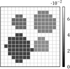
(a) Recovered signal.

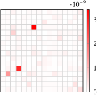
(b) Absolute error.

Figure 1: Masked phase retrieval based on Algorithm 7 with 1 000 iterations and without any modification. The eight masks have been chosen with respect to a Rademacher distribution. Each pixel is covered by at least one mask.

Although the reconstruction is quite accurate, the main drawbacks of a direct application of Proof 7 are the computation time and memory requirements. For 1 000 iterations, we need about 6.38 minutes to recover the true signal. Next, we employ the tensor-free variant of the primal-dual iteration in Proof 11, where we apply the augmented Lanczos bidiagonalization to determine the singular value thresholding (Proof 9). Using this modification, we merely need about 58 seconds to perform the reconstruction. Since we can control the accuracy of the partial singular value decomposition, the performed iteration essentially coincides with the original iteration.

The influence of the augmented Lanczos bidiagonalization on the computation time is presented in Table 1. The parameter $k$ here describes the maximal size of the bidiagonal matrix $\bm{B}_{k}$. Further, $\ell$ denotes the number of fixed Ritz pairs in the augmented restarting procedure. Since the approximation property of the incomplete Lanczos method becomes worse for small $k$, we require more restarts in order to observe an accurate partial singular value decomposition. For higher-dimensional input images, the time saving aspect becomes much more important.

						reweighting
Lanczos vectors $k$	$\infty$	100	50	20	10	10
iteration vectors $\ell$	—	50	25	10	5	5
time in seconds	383.23	139.51	67.94	60.03	57.62	35.74
average restarts	—	0.00	0.06	2.89	10.01	4.89

Table 1: Required computation time for the reconstruction of a $16\times 16$ image by Algorithm 11 with augmented Lanczos process and performing 1 000 iterations.

Considering the evolution of the non-zero singular values of $\bm{w}^{(n)}$ during the iteration, see Table 2, we observe that the projective norm heuristic here enforces a very low rank. After 500 iterations, we nearly obtain a rank-one tensor such that the additional reconstruction error caused by the rank-one projection of $\bm{w}^{(n)}$ to extract the recovered image becomes negligible. After 2 000 iterations, the tensor $\bm{w}^{(n)}$ has converged to a rank-one tensor.

$n$	$\sigma_{0}$		$\sigma_{1}$		$\sigma_{2}$
$100$	$9.89$ $\cdot$	$10^{-1}$	$2.00$ $\cdot$	$10^{-3}$	$6.02$ $\cdot$	$10^{-4}$
$500$	$1.00$ $\cdot$	$10^{\pm 0}$	$7.06$ $\cdot$	$10^{-7}$	$4.59$ $\cdot$	$10^{-7}$
$1\,000$	$1.00$ $\cdot$	$10^{\pm 0}$	$1.13$ $\cdot$	$10^{-10}$
$2\,000$	$1.00$ $\cdot$	$10^{\pm 0}$

Table 2: Evolution of the non-zero singular values using Algorithm 11 with augmented Lanczos  process.

In order to promote the rank-one solutions of the masked Fourier phase retrieval problem even further, we next exploit the reweighting approach proposed in Section 5. For our current simulation, this means that we replace the inner product matrices $\bm{H}=\bm{I}$ by the modified matrices $\bm{H}(\bm{\Xi})$ defined in (22), where we build up the basis $\{\bm{\phi}_{k}\}$ from the singular value decomposition of $\bm{w}^{(n)}$. In the Euclidian setting considered in this simulation, the transformed directions $\widetilde{\bm{\phi}}_{k}$ simply coincide with $\bm{\phi}_{k}$. The reweighting is here applied every ten iterations with relative weight $\lambda\coloneqq\nicefrac{{1}}{{2}}$.

(a) Recovered signal

(b) Absolute error

Figure 2: Masked phase retrieval based on Algorithm 15 incorporating the augmented Lanczos process and the reweighting heuristic. The algorithm is terminated after 1 000 iterations, the reweighting is repeated every 10 iterations with $\lambda\coloneqq\nicefrac{{1}}{{2}}$.

The results of the tensor-free masked Fourier phase retrieval with augmented Lanczos process and Hilbert space reweighting (Proof 15) are shown in Figure 2. Although the reconstruction looks comparable, we want to point out that the absolute errors are several magnitudes smaller. If we compare the evolution of the ranks, see Figure 3, we can see that the proposed reweighting heuristic reduces the rank quite efficiently. More precisely, most of the iterations have rank one. Due to this reduction, the reweighting has also a positive effect on the computation time and the average number of restarts of the Lanczos process, see Table 1. Moreover, we may notice that the data fidelity term $||\hskip 1.0pt\breve{\mathcal{Q}_{\mathfrak{F}}}(\bm{w}^{(n)})-\bm{g}^{\dagger}\hskip 1.0pt||$ decreases with a higher rate. Here the convergences stops after about 650 iterations due to numerical reasons.

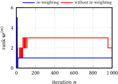
(a) Evolution of the tensor rank.

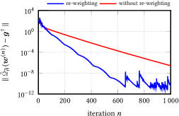
(b) Evolution of the data fidelity term.

Figure 3: Evolution of the rank and data fidelity term during the masked phase retrieval problem based on Algorithm 7 and Algorithm 15.

6.2 Incorporating smoothness properties

One of the central difference between our tensor-free reweighting algorithm and PhaseLift [CSV13, CESV13] consists in the modeling of the domain and image space of the phase retrieval problem. Where PhaseLift is based on the standard Euclidian setting, we rely on arbitrary discrete Hilbert spaces $\mathcal{H}$ and $\mathcal{K}$. Especially, in two-dimensional phase retrieval, we may thus exploit relationships between neighbored pixels like finite differences. More precisely, we here study the influence of the a-priori smoothness property formulated in terms of the two-dimensional discretized Sobolev norm.

In order to discretize the (weighted) Sobolev space $W^{1,2}$, we employ the forward differences

$$\uppartial_{1}\bm{u}[n_{2},n_{1}] \coloneqq\bm{u}[n_{2},n_{1}+1]-\bm{u}[n_{2},n_{1}]\qquad\text{for}\qquad\left\{\begin{aligned} n_{1}&=0,\dots,N_{1}-2\\ n_{2}&=0,\dots,N_{2}-1\end{aligned}\right\}$$

and

$$\uppartial_{2}\bm{u}[n_{2},n_{1}] \coloneqq\bm{u}[n_{2}+1,n_{1}]-\bm{u}[n_{2},n_{1}]\qquad\text{for}\qquad\left\{\begin{aligned} n_{1}&=0,\dots,N_{1}-1\\ n_{2}&=0,\dots,N_{2}-2\end{aligned}\right\}$$

to approximate the first partial derivatives. The associate linear mappings for the vectorized image $\vec{\bm{u}}$ are here denoted by $\bm{D}_{1}$ and $\bm{D}_{2}$. Thus the weighted Sobolev space $\mathcal{H}=W^{1,2}_{\bm{\mu}}$ with weights $\bm{\mu}\coloneqq(\mu_{\bm{I}},\mu_{\bm{D}_{1}},\mu_{\bm{D}_{2}})^{*}$ corresponds to the matrix

$$\bm{H}\coloneqq\mu_{\bm{I}}\,\bm{I}+\mu_{\bm{D}_{1}}\,\bm{D}_{1}^{*}\bm{D}_{1}+\mu_{\bm{D}_{2}}\bm{D}_{2}^{*}\bm{D}_{2}.$$

In comparison, the discretized $L^{2}$-norm corresponds to the standard Euclidian setting associated with the identity matrix.

(a) True signal.

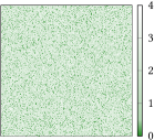
(b) Number of covering Rademacher  masks.

Figure 4: The Fourier data for the second experiment ($256\times 256$ pixels) have been created on the basis of the TEM micrograph of gold nanoparticles [LSP⁺16a, Figure 6C]. The employed masks have again been chosen with respect to the Rademacher distribution. In this instance, about a sixteenth of all pixels are blocked in each of the four masks.

The masked Fourier intensities of the second example has been created on the basis of a transmission electron microscopy (TEM) reconstruction in [LSP⁺16a]. The image has a dimension of $265\times 265$ pixels such that the related tensor possesses $2^{32}$ complex-valued entries and requires 64 GiB memory (double precision complex numbers). Further, we apply four random masks of Rademacher-type (29). Since the masks are generated entirely random, about a one-sixteenth of the pixel are blocked by all masks. The test image together with the number of masks covering a certain pixel are shown in Figure 4.

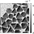
(a) Recovered signal.

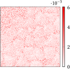
(b) Absolute error.

Figure 5: Masked phase retrieval based on Algorithm 15. The pre-image space $\mathbb{C}^{N_{2}N_{1}}$ is equipped with the discrete $L^{2}$ inner product. The reconstruction is terminated after 100 iterations. In order to compare the retrieval with the true signal, the pixels are presented in the same range as the true image, resulting in the truncation of higher intensities.

(a) Recovered signal.

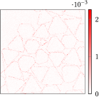
(b) Absolute error.

Figure 6: Masked phase retrieval based on Algorithm 15. The pre-image space $\mathbb{C}^{N_{2}N_{1}}$ is equipped with the discrete Sobolev inner product based on the weight $\bm{\mu}=(0.25,1.00,1.00)^{*}$. The reconstruction is terminated after 100 iterations.

To solve the corresponding masked phase retrieval problem, we apply Proof 15, where we reweight the Hilbert spaces every 10 steps with the relative weight $\lambda\coloneqq\nicefrac{{1}}{{2}}$. Since the algorithm tends to higher-rank tensors in the starting phase, we only compute a partial singular value decomposition with at most five leading singular values using ten Lanczos vectors $\bm{e}_{n}$ and $\bm{f}_{n}$. Hence, we perform Proof 11 in an inexact manner. After a few iterations the rank of $\bm{w}^{(n)}$ decreases such that the method becomes again exact, and that the convergence is ensured.

The reconstructions for the Euclidian and Sobolev setting are presented in Figure 5 and 6, respectively. Due to the small number of four masks, the convergence of the algorithm using the discretized $L^{2}$-norm is very problematic. Although the method converges for the chosen parameters, the convergence rate is very low. Moreover, pixels that are not covered by any masks cannot be recovered and cause reconstruction defects characterized by black holes. Using instead the discretized Sobolev norm with weight $\bm{\mu}\coloneqq(\nicefrac{{1}}{{4}},1,1)$ and the same parameters, we obtain a much faster convergence and rank reduction, see Figure 7. Further, the required number of dual updates in order to produce a non-zero primal update is reduced. A small drawback is that the Sobolev norm tends to smooth out the edges of the particles in the reconstruction. One the other side, the a-priori smoothness condition allows us to recover pixels not covered by the given data.

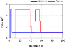
(a) Evolution of the tensor rank.

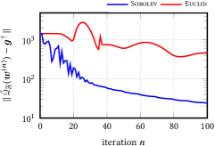
(b) Evolution of the data fidelity term.

Figure 7: Evolution of the rank and data fidelity term during the masked phase retrieval based on Algorithm 15. Both terms are compared for the discrete $L^{2}$ norm (Euclid) and the discrete Sobolev norm with weight $\bm{\mu}=(0.25,1.00,1.00)^{*}$.

6.3 Phase retrieval for large-scale images

Using the proposed reweighting heuristic to reduce the rank of the iteration $\bm{w}^{(n)}$, we are able to perform Proof 15 for much larger test images. In this numerical experiment, we consider an $1\,024\times 1\,024$ pixel image, whose Fourier data are again based on a TEM micrograph of gold nanoparticles [LSP⁺16a]. The lifted image here already requires 16 TiB memory in order to hold the $2^{40}$ complex-valued entries with double precision. Differently from the previous examples, we here apply eight Gaußian masks following the standard normal distribution

$$\bm{d}_{\ell}[n_{2},n_{1}]\sim\mathcal{N}(0,1).\vspace*{5pt}$$

The recovered signal for the Euclidian inner product is shown in Figure 8 together with the evolution of the rank and data fidelity in Figure 9. Analogously to the above experiments, the Hilbert space $\mathcal{H}$ is reweighted every ten iterations with a relative weight $\lambda\coloneqq\nicefrac{{1}}{{2}}$.

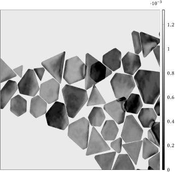
(a) Recovered signal.

(b) Absolute error.

Figure 8: The Fourier data for the third experiment ($1\,024\times 1\,024$ pixels) have been created on the basis of the TEM micrograph [LSP⁺16a, Figure 6B]. The eight masks have been generated regarding a Gaußian distribution. Algorithm 15 has been terminated after 1 000 iterations.

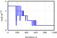
(a) Evolution of the tensor rank.

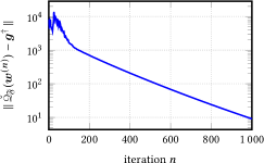
(b) Evolution of the data fidelity term.

Figure 9: Evolution of the rank and data fidelity term during the masked phase retrieval problem based on Algorithm 15 using eight Gaußian masks and terminating after 1 000 iterations.

6.4 Corruption by noise

In the last numerical example, we study the influence of noise to the proposed tensor-free primal-dual algorithm. For simplicity, we only study the behavior of the proposed method with respect to white or Gaußian noise of the form $\bm{g}^{\epsilon}\coloneqq\bm{g}^{\dagger}+\bm{\zeta}$ where $\bm{\zeta}$ is a normal distributed random vector. For the noise level $\epsilon\coloneqq||\hskip 1.0pt\bm{g}^{\dagger}-\bm{g}^{\epsilon}\hskip 1.0pt||$, we consider different percentages of the norm $||\hskip 1.0pt\bm{g}^{\dagger}\hskip 1.0pt||$. Similarly to the first numerical examples, we again apply four Rademacher-type masks of the form (29). The synthetic data $\bm{g}^{\dagger}$ for the $256\times 256$ test image are again based on a TEM reconstruction of gold nanoparticles [LSP⁺16b, Figure S1B] and the $512\times 512$-point Fourier transform. The domain $\mathcal{H}$ is again equipped with the discretized Sobolev norm with weight $\bm{\mu}\coloneqq(\nicefrac{{1}}{{4}},1,1)^{*}$. Due to the noise, we have adapted Proof 15 to the Tikhonov regularization in Proof 7, which simply means that we have to multiply $\bm{y}^{(n+1)}$ in step (ii.a) with $\nicefrac{{1}}{{\sigma+1}}$ additionally and to scale the threshold in step (ii.b) to $\mathcal{S}_{\tau\alpha}$. Since $\alpha$ affects the influence of the projective norm heuristic, this parameter has to be chosen relatively large. In this brief test run with noisy measurements, we chose $\alpha\coloneqq 10^{3}$ independent of the noise level. Surely, the results can be improved by more sophisticated parameter choice rules.

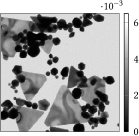
(a) Reconstruction (5%).

(b) Reconstruction (10%).

(c) Reconstruction (25%).

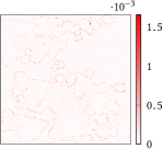
(d) Absolute error (5%).

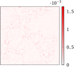
(e) Absolute error (10%).

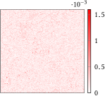
(f) Absolute error (25%).

Figure 10: The influence of noise to masked phase retrieval for a $256\times 256$ test image based on the TEM reconstruction of gold nanoparticles [LSP⁺16b, Figure S1B]. The adaption of Algorithm 15 with respect to the Tikhonov regularization in Algorithm 7 is terminated after 100 iterations.

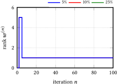
(a) Evolution of the tensor rank.

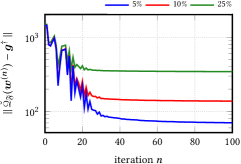
(b) Evolution of the data fidelity term.

Figure 11: Evolution of the rank and data fidelity term during masked phase retrieval for noisy measurements. The noise level is given with respect to the norm $||\hskip 1.0pt\bm{g}^{\dagger}\hskip 1.0pt||$ of the noise-free measurements.

The recovered signals and the evolution of the rank and data fidelity are shown in Figure 10 and 11, respectively. Due to the noise, we cannot ensure that the recovered tensor has rank one and corresponds to a meaningful approximation of the true signal. If we endow the domain $\mathcal{H}$ with the Euclidian inner product in analogy to classical PhaseLift, then we observed that the rank of the iteration $\bm{w}^{(n)}$ increases uncontrollable, and the proposed algorithm diverges because of the limited data provided by only four masks. Using instead the weighted Sobolev norm and the Hilbert space reweighting, the rank becomes one after a short starting phase, where the maximal rank is restricted by five. Because of the same starting value and the same regularization parameter, the primal-dual iteration initially performs nearly identical for the three considered noise levels such that the rank evolutions coincide. Further, for all three cases, we here obtain reasonable reconstructions. Moreover, the pixels not covered by any mask are filled up, and the influence of the noise to the reconstruction is smoothed out. Further numerical experiments suggest that Proof 15 in combination with a-priori smoothness properties recovers the unknown signal in a stable manner.

7 Conclusion

In this paper, we developed a novel proximal algorithm to solve bilinear and quadratic inverse problems. The basic idea was to exploit the universal property to lift the considered problem to linear inverse problems on the tensor product. In order to deal with the rank-one constraint, we applied a nuclear or projective norm heuristic, which is known to produce low-rank solutions. The relaxation of the lifted problem yields a constrained minimization problem, which has been solved by applying the first-order primal-dual algorithm proposed by Chambolle and Pock. Since the choice of the underlying algorithm is somehow arbitrary, there are several further options to develop minimization methods for the lifted and relaxed problem. For instance, one may apply the alternating direction method of multipliers (ADMM) [BPC⁺11], forward-backward splitting [LM79, CW05], or FISTA [BT09].

The flexibility to adapt the domain of the bilinear or quadratic operator allows us to incorporate smoothness assumptions or neighborhood relations. As demonstrated for the masked Fourier phase retrieval problem, this freedom enables us to recover pixels that are blocked by the applied masks such that they do not contribute to the given measurements. Further, the smoothing properties of the discretized Sobolev norm greatly improve the numerical observed convergence rates. Moreover, one can exploit this flexibility to reweight the pre-image spaces in order to promote low-rank solutions. In the moment, we rely on a projective norm based on the corresponding Hilbert norms. Here, the question arises if one can employ nuclear “norms” based on semi-norms like the total variation or total generalized variation.

For the masked Fourier phase retrieval problem, we have shown that the developed algorithms seem to be stable under noise. More precisely, we have studied the influence of white noise, which can be treated by choosing the squared Euclidian or discretized $L^{2}$-norm as data fidelity term of the Tikhonov functional in ($\mathfrak{B}_{\alpha}$) and ($\mathfrak{Q}_{\alpha}$). In order to incorporate more realistic noise models like Poisson noise into phase retrieval, one can, for instance, replace the data fidelity by the Kullback–Leibler divergence. In so doing, one only has to update the proximal mapping to compute the dual variable.

Acknowledgments.  We gratefully acknowledges the funding of this work by the Austrian Science Fund (FWF) within the project P28858. The Institute of Mathematics and Scientific Computing off the University of Graz, with which the authors are affiliated, is a member of NAWI Graz (https://www.nawigraz.at/).

References

[1]
[ABHS16]Anzengruber, Stephan W. ; Bürger, Steven ;
Hofmann, Bernd ; Steinmeyer, Günter:
Variational regularization of complex deautoconvolution and phase
retrieval in ultrashort laser pulse characterization.
In: Inverse Probl 32 (2016), No. 3, pp. 035002(27)
[BB98]Bertero, Mario ; Boccacci, Patrizia:
Introduction to Inverse Problems in Imaging.
Bristol : Institute of Physics Publishing, 1998
[BB18]Beinert, Robert ; Bredies, Kristian:
Non-convex regularization of bilinear and quadratic inverse problems
by tensorial lifting.
In: Inverse Probl 35 (2018), No. 1, pp. 015002
[BBE17]Bendory, Tamir ; Beinert, Robert ; Eldar,
Yonina C.:
Fourier phase retrieval: uniqueness and algorithms.
In: Boche, H. (Ed.) ; Caire, G. (Ed.) ;
Calderbank, R. (Ed.) ; März, M. (Ed.) ;
Kutyniok, G. (Ed.) ; Mathar, R. (Ed.): Compressed
Sensing and its Applications.
Cham : Birkhäser, 2017 (Applied and Numerical Harmonic Analysis),
Chapter 2, pp. 55–91
[BBM+04]Blaimer, M. ; Breuer, F. ; Mueller, M. ;
Heidemann, R. M. ; Griswold, M. A. ; Jakob,
P. M.:
SMASH, SENSE, PILS, GRAPPA: how to choose the optimal method.
In: Top Magn Reson Imaging 15 (2004), No. 4, pp. 233–236
[BP15]Beinert, Robert ; Plonka, Gerlind:
Ambiguities in one-dimensional discrete phase retrieval from Fourier
magnitudes.
In: J Math Anal Appl 21 (2015), No. 6, pp. 1169–1198
[BPC+11]Boyd, Stephen ; Parikh, Neal ; Chu, Eric ;
Peleato, Borja ; Eckstein, Jonathan:
Distributed Optimization and Statistical Learning via the Alternating
Direction Method of Multipliers.
In: Found Trends Mach Learn 3 (2011), No. 1, pp. 1–122
[BS79]Bruck, Yu. M. ; Sodin, L. G.:
On the ambiguity of the image reconstruction problem.
In: Opt Commun 30 (1979), September, No. 3, pp. 304–308
[BS01]Burger, Martin ; Scherzer, Otmar:
Regularization methods for blind deconvolution and blind source
separation problems.
In: Math Control Signals Systems 14 (2001), No. 4, pp.
358–383
[BT09]Beck, Amir ; Teboulle, Marc:
A fast iterative shrinkage-thresholding algorithm for linear inverse
problems.
In: SIAM J Imaging Sci 2 (2009), No. 1, pp. 183–202
[CCS10]Cai, Jian-Feng ; Candès, Emmanuel J. ; Shen,
Zuowei:
A singular value thresholding algorithm for matrix completion.
In: SIAM J Optim 20 (2010), No. 4, pp. 1956–1982
[CESV13]Candès, Emmanuel J. ; Eldar, Yonina C. ;
Strohmer, Thomas ; Voroninski, Vladislav:
Phase retrieval via matrix completion.
In: SIAM J Imaging Sci 6 (2013), No. 1, pp. 199–225
[CLS15]Candès, Emmanuel J. ; Li, Xiaodong ;
Soltanolkotabi, Mahdi:
Phase retrieval from coded diffation patterns.
In: Appl Comput Harmon Anal 39 (2015), No. 2, pp. 277–299
[CP11]Chambolle, Antonin ; Pock, Thomas:
A first-order primal-dual algorithm for convex problems with
applications to imaging.
In: J Math Imaging Vis 40 (2011), No. 1, pp. 120–145
[CP16]Chambolle, Antonin ; Pock, Thomas:
An introduction to continuous optimization for imaging.
In: Acta Numerica 25 (2016), pp. 161–319
[CR09]Candès, Emmanuel J. ; Recht, Benjamin:
Exact matrix completion via convex optimization.
In: Found Comput Math 9 (2009), No. 6, pp. 717–772
[CSV13]Candès, Emmanuel J. ; Strohmer, Thomas ;
Voroninski, Vladislav:
PhaseLift: exact and stable signal recovery from magnitude
measurements via convex programming.
In: Comm Pure Appl Math 66 (2013), No. 8, pp. 1241–1274
[CW05]Combettes, Patrick L. ; Wajs, Valérie R.:
Signal recovery by proximal forward-backward splitting.
In: Multiscale Model. Simul. 4 (2005), No. 4, pp. 1168–1200
[DF87]Dainty, J. C. ; Fienup, J. R.:
Phase retrieval and image reconstruction for astronomy.
In: Stark, Henry (Ed.): Image Recovery :
Theory and Application.
Orlando (Florida) : Academic Press, 1987, Chapter 7, pp. 231–275
[GH94]Gorenflo, Rudolf ; Hofmann, Bernd:
On autoconvolution and regularization.
In: Inverse Probl 10 (1994), No. 2, pp. 353–373
[GHB+14]Gerth, Daniel ; Hofmann, Bernd ; Birkholz, Simon ;
Koke, Sebastian ; Steinmeyer, Günter:
Regularization of an autoconvolution problem in ultrashort laser
pulse characterization.
In: Inverse Probl Sci Eng 22 (2014), No. 2, pp. 245–266
[GK65]Golub, G. ; Kahan, W.:
Calculating the singular values and pseudo-inverse of a matrix.
In: J Soc Indust Appl Math Ser B Numer Anal 2 (1965), No. 2,
pp. 205–224
[GKK17]Gross, David ; Krahmer, Felix ; Kueng, Richard:
Improved recovery guarantees for phase retrieval form coded
diffraction patterns.
In: Appl Comput Harmon Anal 42 (2017), No. 1, pp. 37–64
[GV13]Golub, Gene H. ; Van Loan, Charles F.:
Matrix Computations.
4th edition.
Baltimore : The John Hopkins University Press, 2013 (Johns Hopkins
Studies in the Mathematical Sciences)
[Hau91]Hauptman, Herbert A.:
The phase problem of x-ray crystallography.
In: Rep Prog Phys 54 (1991), November, No. 11, pp.
1427–1454
[Hay82]Hayes, Monson H.:
The reconstruction of a multidimensional sequence from the phase or
magnitude of its Fourier transform.
In: IEEE Trans Acoust Speech Signal Process ASSP-30 (1982),
No. 2, pp. 140–154
[HM82]Hayes, Monson H. ; McClellan, James H.:
Reducible polynomials in more than one variable.
In: Proc IEEE 70 (1982), February, No. 2, pp. 197–198
[JR06]Justen, L. ; Ramlau, R.:
A non-iterative regularization approach to blind deconvolution.
In: Inverse Probl 22 (2006), No. 3, pp. 771–800
[KR83]Kadison, Richard V. ; Ringrose, John R.:
Fundamentals of the Theory of Operator Algebras. Vol. I:
Elementary Theory.
New York : Academic Press, 1983
[LCL+08]Liu, Y. J. ; Chen, B. ; Li, E. R. ; Wang,
J. Y. ; Marcelli, A. ; Wilkins, S. W. ; Ming, H. ;
Tian, Y. C. ; Nugent, K. A. ; Zhu, P. P. ;
Wu, Z. Y.:
Phase retrieval in x-ray imaging based on using structured
illumination.
In: Phys Rev A 78 (2008), August, No. 2, pp. 023817(5)
[Lew95]Lewis, A. S.:
The convex analysis of unitarily invariant matrix functions.
In: J Convex Anal 2 (1995), No. 1/2, pp. 173–183
[Lew96]Lewis, A. S.:
Convex analysis on the Hermitian matrices.
In: SIAM J Optim 6 (1996), No. 1, pp. 164–177
[Lew99]Lewis, A. S.:
Nonsmooth analysis of eigenvalues.
In: Math Program 84 (1999), No. 1, pp. 1–14
[LM79]Lions, P.-L. ; Mercier, B.:
Splitting algorithms for the sum of two nonlinear operators.
In: SIAM J Numer Anal 16 (1979), No. 6, pp. 964–979
[LSP+16a]Liebig, Ferenc ; Sarhan, Radwan M. ; Prietzel,
Claudia ; Reinecke, Antje ; Koetz, Joachim:
‘Green’ gold nanotriangles: synthesis, purification by
polyelectrolyte/micelle depletion flocculation and performance in
surface-enhanced Raman scattering.
In: RSC Adv 6 (2016), pp. 33561–33568. –
Open Access Article licensed under a Creative Commons Attribution 3.0
Unported Licence
[LSP+16b]Liebig, Ferenc ; Sarhan, Radwan M. ; Prietzel,
Claudia ; Reinecke, Antje ; Koetz, Joachim:
‘Green’ gold nanotriangles: synthesis, purification by
polyelectrolyte/micelle depletion flocculation and performance in
surface-enhanced Raman scattering – Supplementary part.
In: RSC Adv 6 (2016), pp. 33561–33568. –
Open Access Article licensed under a Creative Commons Attribution 3.0
Unported Licence
[MGC11]Ma, Shiqian ; Goldfarb, Donald ; Chen, Lifeng:
Fixed point and Bregman iterative methods for matrix rank
minimization.
In: Math Program 128 (2011), No. 1–2, pp. 321–353
[Mil90]Millane, R. P.:
Phase retrieval in crystallography and optics.
In: J Opt Soc Am A 7 (1990), March, No. 3, pp. 394–411
[MS12]Mueller, Jennifer L. ; Siltanen, Samuli:
Linear and Nonlinear Inverse Problems with Practical
Applications.
Philadelphia : SIAM, 2012 (Computational Science & Engineering)
[Ram05]Ramm, Alexander G.:
Inverse problems.
Springer : Springer, 2005 (Mathematical and Analytical Techniques
with Applications to Engineering)
[RFP10]Recht, Benjamin ; Fazel, Maryam ; Parrilo,
Pablo A.:
Guaranteed minimum-rank solutions of linear matrix equations via
nuclear norm minimization.
In: SIAM Rev 52 (2010), No. 3, pp. 471–501
[Roc70]Rockafellar, R. Tyrrell:
Convex Analysis.
Princeton (New Jersey) : Princeton University Press, 1970 (Princeton
Mathematical Series 28)
[RW09]Rockafellar, R. Tyrrell ; Wets, Roger J.-B.:
Variational Analysis.
Dortrecht : Springer, 2009 (Grundlehren der mathematischen
Wissenschaften. A Series of Comprehensive Studies in Mathematics 317)
[Rya02]Ryan, Raymond A.:
Introduction to Tensor Products of Banach Spaces.
London : Springer, 2002 (Springer Monographs in Mathematics)
[SGG+09]Scherzer, Otmar ; Grasmair, Markus ; Grossauer,
Harald ; Haltmeier, Markus ; Lenzen, Frank:
Variational Methods in Imaging.
New York : Springer, 2009
[SSD+06]Seifert, Birger ; Stolz, Heinrich ; Donatelli, Marco
; Langemann, Dirk ; Tasche, Manfred:
Multilevel Gauss-Newton methods for phase retrieval problems.
In: J Phys A: Math Gen 39 (2006), No. 16, pp. 4191–4206
[SST04]Seifert, Birger ; Stolz, Heinrich ; Tasche,
Manfred:
Nontrivial ambiguities for blind frequency-resolved optical gating
and the problem of uniqueness.
In: J Opt Soc Am B 21 (2004), May, No. 5, pp. 1089–1097
[Ste69]Stewart, G. W.:
Accelerating the orthogonal iteration for the eigenvectors of a
Hermitian matrix.
In: Numer Math 13 (1969), No. 4, pp. 362–376
[SW13]Seo, Jin K. ; Woo, Eung J.:
Nonlinear Inverse Problems in Imaging.
Chichester : John Wiley & Sons, 2013
[Uhl03]Uhlmann, Gunther (Ed.):
Mathematical Sciences Research Institute Publications.
Vol. 47: Inside Out: Inverse Problems and Applications.
Cambridge : Cambridge University Press, 2003
[Uhl13]Uhlmann, Gunther (Ed.):
Mathematical Sciences Research Institute Publications.
Vol. 60: Inverse Problems and applications: Inside Out II.
Cambridge : Cambridge University Press, 2013