Spiral-wave wind for the blue kilonova

Abstract

The AT2017gfo kilonova counterpart of the binary neutron star merger event GW170817 was characterized by an early-time bright peak in optical and UV bands. Such blue kilonova is commonly interpreted as a signature of weak $r$-process nucleosynthesis in a fast expanding wind whose origin is currently debated. Numerical-relativity simulations with microphysical equations of state, approximate neutrino transport, and turbulent viscosity reveal a new hydrodynamics-driven mechanism that can power the blue kilonova. Spiral density waves in the remnant generate a characteristic wind of mass ${\sim}10^{-2}~{}{\rm M_{\odot}}$ and velocity ${\sim}0.2$c. The ejected material has electron fraction mostly distributed above $0.25$ being partially reprocessed by hydrodynamic shocks in the expanding arms. The combination of dynamical ejecta and spiral-wave wind can account for solar system abundances of $r$-process elements and early-time observed light curves.

1. Introduction

The observation of the kilonova (kN) AT2017gfo (Coulter et al., 2017; Chornock et al., 2017; Nicholl et al., 2017; Cowperthwaite et al., 2017; Tanvir et al., 2017; Tanaka et al., 2017) associated to the binary neutron star (BNS) merger GW170817 (Abbott et al., 2017) provided evidence that the ejection of neutron-rich matter from compact binary mergers is a primary site for $r$-process nucleosynthesis (Lattimer and Schramm, 1974; Li and Paczynski, 1998; Kulkarni, 2005; Rosswog, 2005; Metzger et al., 2010; Roberts et al., 2011; Kasen et al., 2013). In this scenario, the electromagnetic UV/optical/NIR transient is powered by the radioactive decay of the freshly synthesized elements. The NIR luminosity of AT2017gfo peaked at several days after the merger (Chornock et al., 2017), and it is consistent with expectations that the opacities of expanding $r$-process material are dominated by the opacities of lanthanides and possibly actinides (Kasen et al., 2013). The UV/optical luminosity peaked instead in less than one day after the merger (Nicholl et al., 2017), and it originates from ejected material that experienced only a partial $r$-process nucleosynthesis (Martin et al., 2015). A fit of AT2017gfo light curves to a semianalytical two-components spherical model indicates a lanthanide poor (rich) blue (red) component of mass $2.5\times 10^{-2}M_{\odot}$ ($5.0\times 10^{-2}M_{\odot}$) and velocity $0.27$c ($0.15$c) (Cowperthwaite et al., 2017; Villar et al., 2017) (See however (Waxman et al., 2018) for an alternative interpretation.) Similar results are obtained using more sophisticated 1D simulations of radiation transport along spherical shells of mass ejecta (Tanvir et al., 2017; Tanaka et al., 2017).

Numerical relativity (NR) simulations produce dynamical ejecta of a few times $10^{-3}{\rm M_{\odot}}$ with velocities distributed around ${\sim}0.1{-}0.3$c  (Hotokezaka et al., 2013; Bauswein et al., 2013; Radice et al., 2018a). Dynamical ejecta are characterized by a range of electron fractions $0.05\lesssim Y_{e}\lesssim 0.4$; with larger values distributed towards polar regions above the remnant (as part of the shocked component) and lower values across the equatorial plane. These properties are largely independent of the NS equation of state (EOS) (Sekiguchi et al., 2015; Radice et al., 2018a). Additional ejecta from the disk are expected on longer timescales (Perego et al., 2014; Just et al., 2015; Kasen et al., 2015; Metzger and Fernández, 2014; Wu et al., 2016; Siegel and Metzger, 2017; Fujibayashi et al., 2018; Miller et al., 2019); disk mass and composition depend on the binary mass and EOS (Radice et al., 2018b; Perego et al., 2019). Neutrino irradiation can unbind ${\sim}5$% of the disk mass with $Y_{e}>0.25$ and velocities ${\lesssim}0.08$c from the polar region (Perego et al., 2014; Martin et al., 2015). A significant fraction of the disk mass, up to 40%, can be ejected on time scales ${\gtrsim}100$ ms due to magnetic-field induced viscosity and/or nuclear recombination, (Dessart et al., 2009; Fernández et al., 2015; Wu et al., 2016; Lippuner et al., 2017; Siegel and Metzger, 2017; Fujibayashi et al., 2018; Radice et al., 2018c; Fernández et al., 2019; Miller et al., 2019). These secular ejecta are expected to have velocities ${\lesssim}0.05{-}0.1$c and electron fraction in the broad range $0.1\lesssim Y_{e}\lesssim 0.5$, where lower (higher) values are found for black-hole (long-lived NS) remnant. If present, the secular ejecta might give the dominant contribution to the kN on timescales of days to months (Fahlman and Fernández, 2018).

KN light curve models need to account for multiple ejecta (dynamical, wind, viscous, etc.), for the anisotropy of the ejecta composition, and for the irradiation among the ejecta components to fully explain AT2017gfo. Indeed, outflow properties inferred for AT2017gfo using multi-components and 2D kN models including these effects are broadly compatible with the results from simulations, e.g. (Perego et al., 2017; Kawaguchi et al., 2018). The early blue kN however, remains a challenging aspect to model. Both semi-analytical and radiation transport models require ejecta properties different from those found in simulations. In particular, simulations cannot produce ejecta with the large velocities and electron fraction inferred from the electromagnetic data (Fahlman and Fernández, 2018).

There exist alternative explanations of the blue kN based on the interaction between a relativistic jet and the ejecta (Lazzati et al., 2017; Bromberg et al., 2018; Piro and Kollmeier, 2017) but simulations show that successful jets do not deposit a sufficient amount of thermal energy in the ejecta for this mechanism to work (Duffell et al., 2018). Other possibilities include the presence of highly magnetized winds (Metzger et al., 2018; Fernández et al., 2019), or the presence of the so-called viscous-dynamical ejecta (Radice et al., 2018d). However, both models rely on the development of large-scale strong magnetic fields. Here, we identify a new generic hydrodynamics-driven mechanism that works in self-consistent ab-initio simulations and does not require the presence of a strong ordered magnetic field.

2. Method

Figure 1.— 3D distribution of angular momentum density flux $J_{r}$ from the DD2 simulation with turbulent viscosity at ${\sim}43.5$ ms after merger. $J_{r}$ is shown on a central region of $(89\times 89\times 60)$ km³ covering the remnant NS and disk, and it is given in units where $c=G={\rm M_{\odot}}=1$.

We perform 3+1 NR simulations of two binaries with mass $M=(1.364+1.364){\rm M_{\odot}}$ and NS described by the microphysical EOS HS(DD2) (Typel et al., 2010; Hempel and Schaffner-Bielich, 2010) and LS220 (Lattimer and Swesty, 1991). The simulations include the merger and the remnant evolution for a timescale of at least 30 ms and up to 100 ms depending on the binary. The results presented here are representative cases producing a long-lived NS remnant (DD2) and a short-lived NS (LS220) from a larger set of simulations that will be presented elsewhere.

We use the WhiskyTHC code (Radice and Rezzolla, 2012; Radice et al., 2014a, b, 2018c) with the approximate neutrino transport scheme developed in (Radice et al., 2016a, 2018a). The simulations treat turbulent viscosity using the general-relativistic large eddy simulations method (GRLES) (Radice, 2017). The interactions between the fluid and neutrinos are treated with a leakage scheme in the optically thick regions (Ruffert et al., 1996; Neilsen et al., 2014) while free-streaming neutrinos are evolved according to the M0 scheme discussed in Ref. (Radice et al., 2018a). The turbulent viscosity in the GRLES is parametrized as $\sigma_{T}=\ell_{\rm mix}c_{s}$, where $c_{s}$ is the sound speed and $\ell_{\rm mix}$ is a free parameter that depends on the intensity of the turbulence. We perform two groups of simulations in this work with $\sigma_{T}$ either set to zero, or prescribed as a function of the rest-mass density as in (Perego et al., 2019) using the results of (Kiuchi et al., 2018). We perform simulations with the same grid setup as in Ref. (Radice et al., 2018a). In particular, the adaptive mesh refinement grids have seven 2:1 refinement levels with finest linear resolutions of $h=246,185,123$m, which are labelled LR, SR and HR. Each model was evolved at least at two different resolutions (LR and SR).

The ejecta are calculated on coordinate spheres at $r=294$ km employing the geodesic criterion for the dynamical ejecta (Radice et al., 2018a). For the wind we use the Bernoulli criterion, which is appropriate for steady-state flow, assuming $(\partial_{t})^{a}$ is an approximate Killing vector (see e.g. (Kastaun and Galeazzi, 2015)). The Bernoulli calculation is started after the ejecta mass computed with the geodesic criterion has saturated to its final value. From the fluid’s stress energy tensor, we compute the angular momentum density flux $J_{r}=T_{ra}(\partial_{\phi})^{a}$, where $\phi$ is the cylindrical angular coordinate; angular momentum is conserved if $(\partial_{\phi})^{a}$ is a Killing vector. $r$-process nucleosynthesis yields are computed using the method detailed in (Radice et al., 2018a).

3. Results

The key dynamical feature of relevance here is the development of spiral arms in the remnant (Shibata and Uryu, 2000; Shibata and Taniguchi, 2006; Bernuzzi et al., 2014; Kastaun and Galeazzi, 2015; Bernuzzi et al., 2016; East et al., 2016; Paschalidis et al., 2015; Radice et al., 2016b; Lehner et al., 2016). The hydrodynamic instability is monitored by a decomposition in Fourier modes $e^{-{\rm i}m\phi}$ of the Eulerian rest-mass density on the equatorial plane [see Eq. (1) of (Radice et al., 2016b)] and characterized by the development of a $m=2$ followed by a $m=1$ mode (East et al., 2016; Paschalidis et al., 2015; Radice et al., 2016b; Lehner et al., 2016; Bernuzzi et al., 2014; Kastaun and Galeazzi, 2015). In the short-lived remnant (LS220) the $m=1$ mode is subdominant with respect to the $m=2$, and it reaches a maximum close to the collapse (Bernuzzi et al., 2014). Instead, in the long-lived remnant (DD2) the $m=1$ becomes the dominant mode at $\sim$20 ms and persists throughout the remnant’s lifetime, while the $m=2$ efficiently dissipates via gravitational-wave emission (Bernuzzi et al., 2016; Radice et al., 2016b). Considering the turbulent viscosity effect, we find that the $m=2$ mode is suppressed more rapidly in presence of viscosity than without viscosity. By contrast, the $m=1$ modes are not significantly affected by viscosity. The spiral arms propagate from the remnant NS into the disk and transport angular momentum outwards as shown in Fig. 1. Such global density waves are a generic and efficient mechanism to redistribute energy and eventually deplete accretion disks (Goodman and Rafikov, 2001; Rafikov, 2016; Arzamasskiy and Rafikov, 2018). Crucially, we find that both the $m=1$ and $m=2$ modes generate a spiral-wave wind from the disk’s outer layers that is distinct from the dynamical ejecta, see Fig. 2.

The long lived NS remnant (DD2) develops a spiral-wave wind more massive than the dynamical ejecta, as shown also in Fig. 2. The spiral-wave wind mass is larger the longer the remnant survives and the more massive the disks are. It continues as long as as the remnant does not collapse and the spiral modes persist. Thus, binary mass asymetry can enhance the spiral-wave wind as we find in simulations discussed elsewhere [In Prep.]. The inclusion of turbulent viscosity alters all the ejecta masses with an additional component and, for the viscosity parametrization we have considered, it enhances the DD2 spiral-wave wind mass by ${\sim}25$%. The viscosity effect is larger than resolution effects. Comparing data at different grid resolutions we find that the largest variation is in the wind mass. The relative variation of mass from data pairs at increasing resolutions is ${\sim}+15\%$ (LR-SR) and ${\sim}+8\%$ (SR-HR). Hence, finite grid effects tend to increase mass. A similar analysis on the average electronfraction and velocity indicate variations below $4\%$.

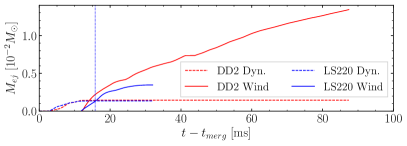
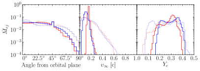
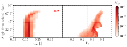
Figure 2.— Properties of the spiral-wave wind and dynamical ejecta computed form the simulations with turbulent viscosity. Top: evolution of unbound mass for dynamical ejecta (dashed lines) and spiral-wave wind (solid lines). $t=0$ marks the moment of merger, the vertical line marks the collapse time of the LS220 BNS. Middle: mass histograms for the angular (left), velocity (center) and electron fraction (right) distributions. Bottom: angular distribution and composition of the spiral-wave wind for DD2. Note the $\bar{M}_{ej}$ in the middle and bottom panels is normalized to one.

The spiral-wave wind has an angular distribution of mass similar to the dynamical ejecta with material mostly confined to the orbital plane, as shown by the histograms in Fig. 2. On the contrary, the velocity profiles show a drastic difference between the two ejecta components. While the dynamical ejecta has a broad velocity distribution (Hotokezaka et al., 2013; Bauswein et al., 2013; Radice et al., 2018a), the spiral-wave wind velocity is narrowly distributed around $0.2$c in the case of a long-lived remnant (DD2). The spiral-wave wind from the short-lived remnant (LS220) has a broader velocity distribution extending down to $0.1$c. This is due to the spiral-wave shutting down and the disk transition to a more steady accretion. As a consequence, the spiral-wave wind ceases but ejecta continue as a slower disc wind driven by nuclear recombination solely. The electron fraction of the spiral-wave wind has a narrower distribution than the dynamical ejecta in both cases. But because disks around NS remnants are less compact, colder, and optically thicker than those around black holes (Perego et al., 2019), the outer layers of the DD2 disk have a lower $Y_{e}$ than the LS220 disk and so does the spiral-wave wind coming from those layers. While the spiral-wave wind is generic in its hydrodynamics origin, the quantification of its properties relies on the accurate microphysics and neutrino treatment in our simulations.

Matter in the spiral-wave wind undergoes $r$-process nucleosynthesis, and produces predominantly elements up to the second peak (mass number $A<130$), see Fig. 3. The combined nucleosynthesis in the dynamical ejecta and the spiral-wave wind reproduces the solar abundances to within the uncertainties due to nuclear physics. The radioactive decay in the spiral-wave wind contributes to a blue day-long kN emission similar to the neutrino wind and viscous ejecta (Perego et al., 2014; Martin et al., 2015; Metzger and Fernández, 2014; Miller et al., 2019). But in comparison to the latter, the spiral-wave wind is distributed closer to the equatorial plane, it is faster and more massive.

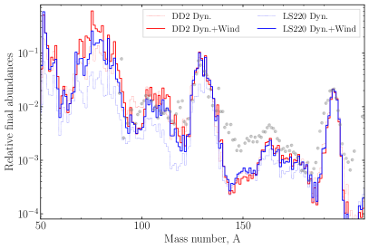
Figure 3.— Nucleosynthetic yields in the ejecta. Dashed lines correspond to the dynamical ejecta, while solid lines are the summed yields including the spiral-wave wind. Model abundances are normalized to $A=195$ element. Gray dots show the solar abundances from Arlandini et al. (1999).

We calculate light curves in different photometric bands by postprocessing the simulation data with the anisotropic multi-component model of (Perego et al., 2017). In order to emulate the spiral-wave wind from different BNS, the DD2 spiral-wave wind data are extracted every $10$ ms until the end of the simulation (${\sim}90$ ms) and then linearly extrapolated to $250$ ms. The LS220 simulation has instead a complete ejecta, since both the dynamical and the spiral-wave wind have terminated at the end of our simulation. We stress that we do not include additional ejecta components to the ones extracted from the simulations, although we expect additional material to be unbound due to viscous processes and nuclear recombination on even longer timescales (Radice et al., 2018c).

Figure 4.— Bolometric kN light curves in three representative bands from blue to infrared for the two simulations with turbulence viscosity compared to AT2017gfo data from (Villar et al., 2017). The color gradient is the effect related to different spiral-wave wind masses, that suggests possible variations of the light curves for different BNS. The band is computed by extracting the spiral-wave wind mass from DD2 every $10$ ms until the end of the simulation, and then by linearly extrapolating the data to $250$ ms.

When comparing our results to the early emission of AT2017gfo in Fig. 4, we find good agreement between the observed luminosities in the high frequency bands and our kN model informed by the DD2 simulation with spiral-wave wind masses ${\sim}0.75{-}1.25\times 10^{-2}M_{\odot}$. By contrast, the LS220 simulation does not produce enough ejecta to explain the observations with this light-curve model. Explaining the low frequency bands with the DD2 data would require a more massive spiral-wave wind with mass ${\gtrsim}2\times 10^{-2}M_{\odot}$, implying a remnant lifetime of ${\gtrsim}200$ ms. However, a more massive spiral-wave wind is incompatible with the early emission for the considered simulations. Late-time luminosities (peaking at $t\approx 3{-}10$ days), could be explained by a combination of spiral-wave wind and viscous ejecta from the disintegration of the disk. These results have uncertainties related to our simplified calculation of the kilonova light curves which is expected to be less accurate at late times when absorption features and deviations from local thermodynamics equilibrium become more relevant, e.g. (Smartt et al., 2017). Indeed, time- and energy-dependent modeling of the photon radiation transport will be needed to model more robustly the kN emission, and quantitatively reproduce the observed spectra (Kasen et al., 2017; Tanaka et al., 2017; Miller et al., 2019; Bulla, 2019). Furthermore, all current kilonova models suffer systematic uncertainties in nuclear (e.g. mass models, fission fragments and $\beta$-decay rates) and atomic (e.g. detailed wavelength dependent opacities for $r$-process element) physics (Eichler et al., 2015; Rosswog et al., 2017; Gaigalas et al., 2019).

4. Conclusion

Standard kN models applied to the early AT2017gfo light curve are in tension with ab-initio simulations conducted so far. While alternative interpretations have been proposed, they are either disfavored by current simulations and observations (e.g. jets) (Bromberg et al., 2018; Duffell et al., 2018), or require the presence of large-scale strong magnetic fields which might not be formed in the postmerger (Metzger et al., 2018; Fernández et al., 2019; Radice et al., 2018d; Ciolfi et al., 2019). We identified a robust dynamical mechanism for mass ejection that explains early-time observations without requiring any fine-tuning. The resulting nucleosynthesis is complete and produces all $r$-process elements in proportions similar to solar system abundances. Methodologically, our work underlines the importance of employing NR-informed ejecta for the fitting of light-curves. Further work in this direction should include better neutrino-radiation transport and magnetohydrodynamic effects (Siegel and Metzger, 2017; Fujibayashi et al., 2018; Radice et al., 2018c, a; Miller et al., 2019).

References

- Coulter et al. (2017) D. A. Coulter et al., Science (2017), 10.1126/science.aap9811, [Science358,1556(2017)], arXiv:1710.05452 [astro-ph.HE] .
- Chornock et al. (2017) R. Chornock et al., Astrophys. J. 848, L19 (2017), arXiv:1710.05454 [astro-ph.HE] .
- Nicholl et al. (2017) M. Nicholl et al., Astrophys. J. 848, L18 (2017), arXiv:1710.05456 [astro-ph.HE] .
- Cowperthwaite et al. (2017) P. S. Cowperthwaite et al., Astrophys. J. 848, L17 (2017), arXiv:1710.05840 [astro-ph.HE] .
- Tanvir et al. (2017) N. R. Tanvir et al., Astrophys. J. 848, L27 (2017), arXiv:1710.05455 [astro-ph.HE] .
- Tanaka et al. (2017) M. Tanaka et al., Publ. Astron. Soc. Jap. (2017), 10.1093/pasj/psx121, arXiv:1710.05850 [astro-ph.HE] .
- Abbott et al. (2017) B. P. Abbott et al. (Virgo, LIGO Scientific), Phys. Rev. Lett. 119, 161101 (2017), arXiv:1710.05832 [gr-qc] .
- Lattimer and Schramm (1974) J. M. Lattimer and D. N. Schramm, apjl 192, L145 (1974).
- Li and Paczynski (1998) L.-X. Li and B. Paczynski, Astrophys.J. 507, L59 (1998), arXiv:astro-ph/9807272 [astro-ph] .
- Kulkarni (2005) S. R. Kulkarni, (2005), arXiv:astro-ph/0510256 [astro-ph] .
- Rosswog (2005) S. Rosswog, Astrophys. J. 634, 1202 (2005), arXiv:astro-ph/0508138 [astro-ph] .
- Metzger et al. (2010) B. Metzger, G. Martinez-Pinedo, S. Darbha, E. Quataert, A. Arcones, et al., Mon.Not.Roy.Astron.Soc. 406, 2650 (2010), arXiv:1001.5029 [astro-ph.HE] .
- Roberts et al. (2011) L. F. Roberts, D. Kasen, W. H. Lee, and E. Ramirez-Ruiz, Astrophys.J. 736, L21 (2011), arXiv:1104.5504 [astro-ph.HE] .
- Kasen et al. (2013) D. Kasen, N. R. Badnell, and J. Barnes, Astrophys. J. 774, 25 (2013), arXiv:1303.5788 [astro-ph.HE] .
- Martin et al. (2015) D. Martin, A. Perego, A. Arcones, F.-K. Thielemann, O. Korobkin, and S. Rosswog, Astrophys. J. 813, 2 (2015), arXiv:1506.05048 [astro-ph.SR] .
- Villar et al. (2017) V. A. Villar et al., Astrophys. J. 851, L21 (2017), arXiv:1710.11576 [astro-ph.HE] .
- Waxman et al. (2018) E. Waxman, E. O. Ofek, D. Kushnir, and A. Gal-Yam, Mon. Not. Roy. Astron. Soc. 481, 3423 (2018), arXiv:1711.09638 [astro-ph.HE] .
- Hotokezaka et al. (2013) K. Hotokezaka, K. Kiuchi, K. Kyutoku, H. Okawa, Y.-i. Sekiguchi, et al., Phys.Rev. D87, 024001 (2013), arXiv:1212.0905 [astro-ph.HE] .
- Bauswein et al. (2013) A. Bauswein, S. Goriely, and H.-T. Janka, Astrophys.J. 773, 78 (2013), arXiv:1302.6530 [astro-ph.SR] .
- Radice et al. (2018a) D. Radice, A. Perego, K. Hotokezaka, S. A. Fromm, S. Bernuzzi, and L. F. Roberts, Astrophys. J. 869, 130 (2018a), arXiv:1809.11161 [astro-ph.HE] .
- Sekiguchi et al. (2015) Y. Sekiguchi, K. Kiuchi, K. Kyutoku, and M. Shibata, Phys.Rev. D91, 064059 (2015), arXiv:1502.06660 [astro-ph.HE] .
- Perego et al. (2014) A. Perego, S. Rosswog, R. Cabezon, O. Korobkin, R. Kaeppeli, et al., Mon.Not.Roy.Astron.Soc. 443, 3134 (2014), arXiv:1405.6730 [astro-ph.HE] .
- Just et al. (2015) O. Just, A. Bauswein, R. A. Pulpillo, S. Goriely, and H. T. Janka, Mon. Not. Roy. Astron. Soc. 448, 541 (2015), arXiv:1406.2687 [astro-ph.SR] .
- Kasen et al. (2015) D. Kasen, R. Fernández, and B. Metzger, Mon. Not. Roy. Astron. Soc. 450, 1777 (2015), arXiv:1411.3726 [astro-ph.HE] .
- Metzger and Fernández (2014) B. D. Metzger and R. Fernández, Mon.Not.Roy.Astron.Soc. 441, 3444 (2014), arXiv:1402.4803 [astro-ph.HE] .
- Wu et al. (2016) M.-R. Wu, R. Fernández, G. Martínez-Pinedo, and B. D. Metzger, Mon. Not. Roy. Astron. Soc. 463, 2323 (2016), arXiv:1607.05290 [astro-ph.HE] .
- Siegel and Metzger (2017) D. M. Siegel and B. D. Metzger, Phys. Rev. Lett. 119, 231102 (2017), arXiv:1705.05473 [astro-ph.HE] .
- Fujibayashi et al. (2018) S. Fujibayashi, K. Kiuchi, N. Nishimura, Y. Sekiguchi, and M. Shibata, Astrophys. J. 860, 64 (2018), arXiv:1711.02093 [astro-ph.HE] .
- Miller et al. (2019) J. M. Miller, B. R. Ryan, J. C. Dolence, A. Burrows, C. J. Fontes, C. L. Fryer, O. Korobkin, J. Lippuner, M. R. Mumpower, and R. T. Wollaeger, Phys. Rev. D100, 023008 (2019), arXiv:1905.07477 [astro-ph.HE] .
- Radice et al. (2018b) D. Radice, A. Perego, F. Zappa, and S. Bernuzzi, Astrophys. J. 852, L29 (2018b), arXiv:1711.03647 [astro-ph.HE] .
- Perego et al. (2019) A. Perego, S. Bernuzzi, and D. Radice, Eur. Phys. J. A55, 124 (2019), arXiv:1903.07898 [gr-qc] .
- Dessart et al. (2009) L. Dessart, C. Ott, A. Burrows, S. Rosswog, and E. Livne, Astrophys.J. 690, 1681 (2009), arXiv:0806.4380 [astro-ph] .
- Fernández et al. (2015) R. Fernández, E. Quataert, J. Schwab, D. Kasen, and S. Rosswog, Mon. Not. Roy. Astron. Soc. 449, 390 (2015), arXiv:1412.5588 [astro-ph.HE] .
- Lippuner et al. (2017) J. Lippuner, R. Fernández, L. F. Roberts, F. Foucart, D. Kasen, B. D. Metzger, and C. D. Ott, Mon. Not. Roy. Astron. Soc. 472, 904 (2017), arXiv:1703.06216 [astro-ph.HE] .
- Radice et al. (2018c) D. Radice, A. Perego, S. Bernuzzi, and B. Zhang, Mon. Not. Roy. Astron. Soc. 481, 3670 (2018c), arXiv:1803.10865 [astro-ph.HE] .
- Fernández et al. (2019) R. Fernández, A. Tchekhovskoy, E. Quataert, F. Foucart, and D. Kasen, Mon. Not. Roy. Astron. Soc. 482, 3373 (2019), arXiv:1808.00461 [astro-ph.HE] .
- Fahlman and Fernández (2018) S. Fahlman and R. Fernández, Astrophys. J. 869, L3 (2018), arXiv:1811.08906 [astro-ph.HE] .
- Perego et al. (2017) A. Perego, D. Radice, and S. Bernuzzi, Astrophys. J. 850, L37 (2017), arXiv:1711.03982 [astro-ph.HE] .
- Kawaguchi et al. (2018) K. Kawaguchi, M. Shibata, and M. Tanaka, Astrophys. J. 865, L21 (2018), arXiv:1806.04088 [astro-ph.HE] .
- Lazzati et al. (2017) D. Lazzati, A. Deich, B. J. Morsony, and J. C. Workman, Mon. Not. Roy. Astron. Soc. 471, 1652 (2017), arXiv:1610.01157 [astro-ph.HE] .
- Bromberg et al. (2018) O. Bromberg, A. Tchekhovskoy, O. Gottlieb, E. Nakar, and T. Piran, Mon. Not. Roy. Astron. Soc. 475, 2971 (2018), arXiv:1710.05897 [astro-ph.HE] .
- Piro and Kollmeier (2017) A. L. Piro and J. A. Kollmeier, (2017), arXiv:1710.05822 [astro-ph.HE] .
- Duffell et al. (2018) P. C. Duffell, E. Quataert, D. Kasen, and H. Klion, Astrophys. J. 866, 3 (2018), arXiv:1806.10616 [astro-ph.HE] .
- Metzger et al. (2018) B. D. Metzger, T. A. Thompson, and E. Quataert, Astrophys. J. 856, 101 (2018), arXiv:1801.04286 [astro-ph.HE] .
- Radice et al. (2018d) D. Radice, A. Perego, K. Hotokezaka, S. Bernuzzi, S. A. Fromm, and L. F. Roberts, Astrophys. J. Lett. 869, L35 (2018d), arXiv:1809.11163 [astro-ph.HE] .
- Typel et al. (2010) S. Typel, G. Ropke, T. Klahn, D. Blaschke, and H. H. Wolter, Phys. Rev. C81, 015803 (2010), arXiv:0908.2344 [nucl-th] .
- Hempel and Schaffner-Bielich (2010) M. Hempel and J. Schaffner-Bielich, Nucl. Phys. A837, 210 (2010), arXiv:0911.4073 [nucl-th] .
- Lattimer and Swesty (1991) J. M. Lattimer and F. D. Swesty, Nucl. Phys. A535, 331 (1991).
- Radice and Rezzolla (2012) D. Radice and L. Rezzolla, Astron. Astrophys. 547, A26 (2012), arXiv:1206.6502 [astro-ph.IM] .
- Radice et al. (2014a) D. Radice, L. Rezzolla, and F. Galeazzi, Mon.Not.Roy.Astron.Soc. 437, L46 (2014a), arXiv:1306.6052 [gr-qc] .
- Radice et al. (2014b) D. Radice, L. Rezzolla, and F. Galeazzi, Class.Quant.Grav. 31, 075012 (2014b), arXiv:1312.5004 [gr-qc] .
- Radice et al. (2016a) D. Radice, F. Galeazzi, J. Lippuner, L. F. Roberts, C. D. Ott, and L. Rezzolla, Mon. Not. Roy. Astron. Soc. 460, 3255 (2016a), arXiv:1601.02426 [astro-ph.HE] .
- Radice (2017) D. Radice, Astrophys. J. 838, L2 (2017), arXiv:1703.02046 [astro-ph.HE] .
- Ruffert et al. (1996) M. H. Ruffert, H. T. Janka, and G. Schäfer, Astron. Astrophys. 311, 532 (1996), arXiv:astro-ph/9509006 .
- Neilsen et al. (2014) D. Neilsen, S. L. Liebling, M. Anderson, L. Lehner, E. O’Connor, et al., Phys.Rev. D89, 104029 (2014), arXiv:1403.3680 [gr-qc] .
- Kiuchi et al. (2018) K. Kiuchi, K. Kyutoku, Y. Sekiguchi, and M. Shibata, Phys. Rev. D97, 124039 (2018), arXiv:1710.01311 [astro-ph.HE] .
- Kastaun and Galeazzi (2015) W. Kastaun and F. Galeazzi, Phys.Rev. D91, 064027 (2015), arXiv:1411.7975 [gr-qc] .
- Shibata and Uryu (2000) M. Shibata and K. Uryu, Phys. Rev. D61, 064001 (2000), arXiv:gr-qc/9911058 .
- Shibata and Taniguchi (2006) M. Shibata and K. Taniguchi, Phys.Rev. D73, 064027 (2006), arXiv:astro-ph/0603145 [astro-ph] .
- Bernuzzi et al. (2014) S. Bernuzzi, T. Dietrich, W. Tichy, and B. Brügmann, Phys.Rev. D89, 104021 (2014), arXiv:1311.4443 [gr-qc] .
- Bernuzzi et al. (2016) S. Bernuzzi, D. Radice, C. D. Ott, L. F. Roberts, P. Moesta, and F. Galeazzi, Phys. Rev. D94, 024023 (2016), arXiv:1512.06397 [gr-qc] .
- East et al. (2016) W. E. East, V. Paschalidis, F. Pretorius, and S. L. Shapiro, Phys. Rev. D93, 024011 (2016), arXiv:1511.01093 [astro-ph.HE] .
- Paschalidis et al. (2015) V. Paschalidis, W. E. East, F. Pretorius, and S. L. Shapiro, Phys. Rev. D92, 121502 (2015), arXiv:1510.03432 [astro-ph.HE] .
- Radice et al. (2016b) D. Radice, S. Bernuzzi, and C. D. Ott, Phys. Rev. D94, 064011 (2016b), arXiv:1603.05726 [gr-qc] .
- Lehner et al. (2016) L. Lehner, S. L. Liebling, C. Palenzuela, and P. M. Motl, Phys. Rev. D94, 043003 (2016), arXiv:1605.02369 [gr-qc] .
- Goodman and Rafikov (2001) J. Goodman and R. R. Rafikov, Astrophys. J. 552, 793 (2001), astro-ph/0010576 .
- Rafikov (2016) R. R. Rafikov, Astrophys. J. 831, 122 (2016), arXiv:1601.03009 [astro-ph.EP] .
- Arzamasskiy and Rafikov (2018) L. Arzamasskiy and R. R. Rafikov, Astrophys. J. 854, 84 (2018), arXiv:1710.01304 [astro-ph.EP] .
- Arlandini et al. (1999) C. Arlandini, F. Kaeppeler, K. Wisshak, R. Gallino, M. Lugaro, M. Busso, and O. Straniero, Astrophys. J. 525, 886 (1999), arXiv:astro-ph/9906266 [astro-ph] .
- Smartt et al. (2017) S. J. Smartt et al., Nature (2017), 10.1038/nature24303, arXiv:1710.05841 [astro-ph.HE] .
- Kasen et al. (2017) D. Kasen, B. Metzger, J. Barnes, E. Quataert, and E. Ramirez-Ruiz, Nature (2017), 10.1038/nature24453, [Nature551,80(2017)], arXiv:1710.05463 [astro-ph.HE] .
- Bulla (2019) M. Bulla, Mon. Not. Roy. Astron. Soc. 489, 5037 (2019), arXiv:1906.04205 [astro-ph.HE] .
- Eichler et al. (2015) M. Eichler et al., Astrophys. J. 808, 30 (2015), arXiv:1411.0974 [astro-ph.HE] .
- Rosswog et al. (2017) S. Rosswog, U. Feindt, O. Korobkin, M. R. Wu, J. Sollerman, A. Goobar, and G. Martinez-Pinedo, Class. Quant. Grav. 34, 104001 (2017), arXiv:1611.09822 [astro-ph.HE] .
- Gaigalas et al. (2019) G. Gaigalas, D. Kato, P. Rynkun, L. Radziute, and M. Tanaka, Astrophys. J. Suppl. 240, 29 (2019), arXiv:1901.10671 [astro-ph.SR] .
- Ciolfi et al. (2019) R. Ciolfi, W. Kastaun, J. V. Kalinani, and B. Giacomazzo, Phys. Rev. D100, 023005 (2019), arXiv:1904.10222 [astro-ph.HE] .