Deciphering the $z_{g}$ distribution in ultrarelativistic heavy ion collisions

Abstract

Within perturbative QCD, we develop a new picture for the parton shower generated by a jet propagating through a dense quark-gluon plasma. This picture combines in a simple, factorised, way multiple medium-induced parton branchings and standard vacuum-like emissions, with the phase-space for the latter constrained by the presence of the medium. We implement this picture as a Monte Carlo generator that we use to study two phenomenologically important observables: the jet nuclear modification factor $R_{AA}$ and the $z_{g}$ distribution reflecting the jet substructure. In both cases, the outcome of our Monte Carlo simulations is in good agreement with the LHC measurements. We provide basic analytic calculations that help explaining the main features observed in the data. We find that the energy loss by the jet is increasing with the jet transverse momentum, due to a rise in the number of partonic sources via vacuum-like emissions. This is a key element in our description of both $R_{AA}$ and the $z_{g}$ distribution. For the latter, we identify two main nuclear effects: incoherent jet energy loss and hard medium-induced emissions. As the jet transverse momentum increases, we predict a qualitative change in the ratio between the $z_{g}$ distributions in PbPb and pp collisions: from increasing at small $z_{g}$, this ratio becomes essentially flat, or even slightly decreasing.

We want to dedicate this paper to the 80${}^{\text{th}}$ birthday of Al Mueller, who pioneered the studies of jet quenching in perturbative QCD and was also our collaborator on a previous paper which introduced the general physical picture that we further develop in this work.

1 Introduction

“Jet quenching” is a rather generic denomination for the ensemble of nuclear modifications affecting a highly-energetic jet or hadron propagating through the dense partonic medium created in ultrarelativistic heavy ion collisions. Its study at RHIC and at the LHC is one of the main sources of information about the deconfined, quark-gluon plasma, phase of QCD. It is associated with a rich and complex phenomenology which includes a broad range of observables, from very inclusive one like the “nuclear modification factor” $R_{AA}$ (for hadrons or jets), to more detailed ones like the jet shape, the jet fragmentation function and jet substructure. These observables are both delicate to measure (e.g. due to the complexity of the background) and delicate to interpret theoretically (due to the high density of partons and their interplay with various collective, non-perturbative, phenomena). In this context, it is difficult to build a full theoretical picture of jet quenching from first principles, although a few specific phenomena have been described using (or at least taking inspiration from) perturbative QCD (pQCD). We refer for example to the recent reviews Mehtar-Tani:2013pia ; Blaizot:2015lma ; Qin:2015srf .

Jet substructure observables have attracted a lot of attention recently, due to their potential to capture detailed aspects of the dynamics of jet quenching (see e.g. Andrews:2018jcm for a recent review and more references). This paper focuses on the “$z_{g}$ distribution” Larkoski:2015lea , where $z_{g}$ is the splitting fraction of the first hard splitting selected by the Soft Drop (SD) procedure Larkoski:2014wba . This observable may reveal the nuclear modification effects on the parton splitting functions. In nucleus-nucleus ($AA$) collisions experimental studies at the LHC, by CF’S Sirunyan:2017bsd and ALICE Acharya:2019djg , reported significant nuclear effects in the $z_{g}$ distribution. Expectations on the theoretical side are less obvious and the main goal of this paper is to highlight the jet quenching mechanisms controlling the $z_{g}$ distribution (see also Refs. Chien:2016led ; Mehtar-Tani:2016aco ; Chang:2017gkt ; Milhano:2017nzm ).

Since the SD procedure clusters the constituents of the jet with the Cambridge/Aachen algorithm Dokshitzer:1997in ; Wobisch:1998wt (see Sect. 22 below for details), it is intrinsically built with the expectation of angular ordering (AO) between successive parton branchings. This property follows from the colour coherence of parton splittings Dokshitzer:1991wu and is at the heart of partonic cascades in $pp$ collisions. One reason why the $z_{g}$ distribution is difficult to describe theoretically in $AA$ collisions is that angular ordering is expected to be violated. This is certainly the case for the medium-induced emissions (MIEs), the parton branchings triggered by collisions with the medium constituents Baier:1996kr ; Baier:1996sk ; Zakharov:1996fv ; Zakharov:1997uu ; Baier:1998kq . As shown in Refs. MehtarTani:2010ma ; MehtarTani:2011tz ; CasalderreySolana:2011rz ; Blaizot:2012fh ; Blaizot:2013vha ; Apolinario:2014csa , these collisions wash out the quantum coherence between the daughter partons produced by a MIE, thus suppressing the interference effects responsible for angular ordering. A priori, the collisions can also affect the partons produced via vacuum-like emissions (VLEs) — the standard bremsstrahlung triggered by the parton virtualities — occurring inside the medium.

The situation of VLEs has been clarified recently in Ref. Caucal:2018dla , which demonstrated that the VLEs occurring inside the medium do still obey AO, essentially because they occur too fast to be influenced by the collisions. The only effect of the medium is to restrict the phase-space available for VLEs.

The same argument implies that the vacuum-like emissions can be factorised in time from the medium-induced radiations, at least within the limits of a leading double-logarithmic approximation (DLA) in which the successive branchings are strongly ordered in both energies and angles. This picture, derived from first principles, allows for a Monte Carlo implementation of the parton showers produced in $AA$ collisions. In this picture, VLEs (satisfying angular ordering) and MIEs (for which quantum coherence can be neglected) are factorised and are both described by a Markovian process.

The phenomenological discussions in Ref. Caucal:2018dla only included VLEs at DLA. To have a chance to be realistic, several extensions are necessary. First, it must include medium-induced radiation and transverse momentum broadening. These higher twist effects carry particles to large angles and are responsible for the energy loss by the jet. Second, it must include the complete (leading-order) DGLAP splitting functions for the VLEs, to have a more realistic description for the energy flow in the cascade and to ensure energy conservation. This also means that one must go beyond the DLA, by giving up the strong ordering in energies at the emission vertices.

We will show in this paper that the factorised picture still holds in a single logarithmic approximation in which successive VLEs are strongly ordered in angles. We will then provide a corresponding Monte Carlo implementation. In this implementation, the medium-induced radiation will be treated in the spirit of the effective theory developed in Refs. Blaizot:2012fh ; Blaizot:2013hx ; Blaizot:2013vha ; Fister:2014zxa , i.e. as a sequence of independent emissions occurring at a rate given by the BDMPS-Z spectrum Baier:1996kr ; Baier:1996sk ; Zakharov:1996fv ; Zakharov:1997uu ; Baier:1998kq . This is the right approximation for the relatively soft MIEs that we are primarily interested in this work.

In this first study, our description of the medium will be oversimplified: we assume a fixed “brick” of size $L$, the distance travelled by the jet inside the medium, and characterised by a uniform value for the jet quenching parameter $\hat{q}$, the rate for transverse momentum broadening via elastic collisions. This description can certainly be improved in the future, e.g. by including the longitudinal expansion of the medium as a time-dependence in $\hat{q}$. Given these simplifying assumptions, we concentrate on observables which, in our opinion, are mainly controlled by the parton showers and which are mostly sensitive to global properties of the medium, like the typical energy loss by a jet (which scales like $\hat{q}L^{2}$) or the typical transverse momentum acquired via elastic collisions (the “saturation momentum” $Q_{s}^{2}\equiv\hat{q}L$). At least in our theoretical approach, this is the case for observables like the jet nuclear modification factor $R_{AA}$ and the $z_{g}$ distribution. This is further supported by the good agreement that we shall find between our results and the corresponding LHC data.

As a baseline for discussion, we will study the jet nuclear modification factor $R_{AA}$. Comparing our predictions to the ATLAS measurements Aaboud:2018twu will allow us to calibrate our medium parameters $\hat{q}$ and $L$ (and a coupling $\alpha_{s,\text{med}}$). We will find that the dependence of $R_{AA}$ on the jet transverse momentum $p_{T}$ is controlled by the evolution of the parton multiplicity via VLEs inside the medium. Each of these partons then acts as a source for medium-induced radiation, enhancing the jet energy loss as $p_{T}$ increases. We shall notably check that $R_{AA}$ is primarily controlled by the energy scale $\omega_{\text{br}}\equiv\alpha_{s,\text{med}}^{2}\hat{q}L^{2}/2$ (the characteristic scale for multiple medium-induced branchings).

The $z_{g}$-distribution is an observable particularly suited for our purposes. On one hand, it is associated with relatively hard branchings, for which perturbative QCD is expected to be applicable. On the other hand, it is sensitive to the dynamics of the MIEs, that are probed both directly (especially at relatively small values of $z_{g}$, where the SD procedure can select a MIE) and indirectly (via the energy loss of the subjets produced by a hard vacuum-like branching).

Our purpose is to provide a transparent physical interpretation and a qualitative description of the relevant LHC data Sirunyan:2017bsd ; Acharya:2019djg . To that aim, we also construct piecewise analytic approximations, whose results are eventually compared to our numerical simulations. In this process, two natural kinematic regimes will emerge, “low energy” and “high energy”, with the transition between them occurring around $p_{T}=\hat{q}L^{2}/(2z_{\text{cut}})$. Here, $z_{\text{cut}}$ is the lower limit on $z_{g}$ which is used by the SD algorithm, that we shall chose as $z_{\text{cut}}=0.1$ in our explicit calculations, in compliance with the experimental measurements in Sirunyan:2017bsd ; Acharya:2019djg . For a “high energy jet”, the SD procedure can only select a vacuum-like splitting, so the only nuclear effect is the (incoherent) energy loss of the two subjets created by this splitting. For “low energy jets”, both VLEs and MIEs can be captured by SD and the contribution from the MIEs leads a significant rise in the $z_{g}$ distribution at small $z_{g}$.

From this perspective, the current measurements of the $z_{g}$-distribution at RHIC Kauder:2017cvz and the LHC Sirunyan:2017bsd ; Acharya:2019djg belong to the low energy regime. Our predictions reproduce the trends seen in the LHC data, both qualitatively and semi-quantitatively (see the discussion in Sect. 6, notably Figures 18 to 22). We argue that the onset of the transition between the low- and high-energy regimes is already visible in the current LHC data (in the highest energy bin, with 300 GeV$\ <p_{T}<500$ GeV) and that the change in behaviour should become even more visible when further increasing $p_{T}$

Given the importance of the jet energy loss for both the $z_{g}$-distribution and the nuclear modification factor $R_{AA}$, we propose a new measurement to study the correlation between these two observables. The idea is to measure the jet $R_{AA}$ as a function of the jet $p_{T}$ in bins of $z_{g}$ or, even better, in bins of $\theta_{g}$ (the angular separation between the two subjets identified by SD). We find (see Sect. 6.3 and, in particular Fig. 23), a larger suppression of $R_{AA}$, meaning a larger energy loss, for 2-prong jets which have passed the SD criteria than for the 1-prong jets which did not.

This paper is structured as follows: Sect. 2 describes the general physical picture and the underlying approximations. We start with a brief summary of the argument for the factorisation of the in-medium parton shower as originally formulated in Ref. Caucal:2018dla and then explain the extension of this argument beyond DLA. Sect. 3 presents the Monte Carlo implementation of this factorised picture. We begin the discussion of our new results in Sect. 4, where we study the jet energy loss and present our predictions for the jet $R_{AA}$. The next two sections present an extensive study of the nuclear effects on the $z_{g}$-distribution. In Sect. 5, we consider “monochromatic” jets generated by a leading parton (gluon or quark) with a fixed energy $p_{T}$. To uncover the physics underlying the $z_{g}$ distribution, we construct analytic calculations that we compare to our Monte Carlo results. In Sect. 6, we move to our phenomenological predictions using a full matrix element for the production of the leading partons. We compare our numerical results with the experimental analyses of the LHC data Sirunyan:2017bsd ; Acharya:2019djg , whenever applicable. Finally, Sect. 7 presents our conclusions together with open problems and perspectives.

2 Parton shower in the medium: physical picture

In this section, we describe our factorised pQCD picture for the parton shower generated by an energetic parton propagating through a homogeneous dense QCD medium of size $L$. We discuss the validity of this picture beyond the double-logarithmic approximation originally used in Ref. Caucal:2018dla .

2.1 Basic considerations

We aim at describing jets created in ultrarelativistic heavy ion collisions and which propagate at nearly central rapidities (the most interesting situation for the physics of jet quenching). For such jets, one can identify the energy and the transverse momentum (w.r.t. the collision axis), so in what follows we use these notations interchangeably. In particular, the energy of the leading parton (quark or gluon) initiating the jet will be interchangeably denoted by $E$ or $p_{T0}$.

The leading parton is created with a time-like virtuality $Q^{2}\ll E^{2}$ via a hard $2\to 2$ partonic process. In the “vacuum” (i.e. in a proton-proton collision), such a parton typically decays after a time of the order of the formation time $t_{\rm f}\equiv 1/\Delta E$. Using $\Delta E=\sqrt{E^{2}+Q^{2}}-E\simeq Q^{2}/2E$, we have

$$t_{\rm f}\,\simeq\,\frac{2E}{Q^{2}}\,\simeq\,\frac{2}{z(1-z)E\theta^{2}}\,\simeq\,\frac{2z(1-z)E}{k_{\perp}^{2}}\,,$$ (1)

where $z$ and $\theta$ (assuming $\theta\ll 1$) are the energy fraction and opening angle of the partonic decay and $k_{\perp}\simeq z(1-z)\theta E$ is the (relative) transverse momentum of any of the two daughter partons w.r.t. the direction of the leading parton.

The differential probability for vacuum-like branching is then given by the bremsstrahlung law,

$${\rm d}^{2}\mathcal{P}_{\text{vac}}\,=\,\frac{\alpha_{s}(k_{\perp}^{2})}{2\pi}\,\frac{{\rm d}^{2}\bm{k}_{\perp}}{\bm{k}_{\perp}^{2}}\,P_{a\to bc}(z)\,{\rm d}z\,=\,\frac{\alpha_{s}(k_{\perp}^{2})}{2\pi}\,\frac{{\rm d}\theta^{2}}{\theta^{2}}\,P_{a\to bc}(z)\,{\rm d}z\,,$$ (2)

where $P_{a\to bc}$ is the Altarelli-Parisi splitting function for the branching of a parton of type $a$ into two partons of type $b$ and $c$ with energy fractions $z$ and respectively $1-z$. The second equality above holds after averaging over the azimuthal angle $\phi$ (the orientation of the 2-dimensional vector $\bm{k}_{\perp}$). For physics discussions, it is often helpful to consider the limit $z\ll 1$ where the emitted gluon is soft. In this case, $P(z)\simeq 2C_{R}/z$ — with $C_{R}=C_{F}=(N_{c}^{2}-1)/(2N_{c})$ for quarks and $C_{R}=C_{A}=N_{c}$ for gluons — and we can write $t_{\rm f}\simeq 2/(\omega\theta^{2})$ and $k_{\perp}\simeq\omega\theta$, with $\omega\equiv zE\ll E$.

In the presence of a medium, additional effects have to be taken into account as high-energy partons traversing the medium suffer elastic collisions and thus receive transverse kicks. This has three main consequences: (i) they affect the available phase-space for vacuum-like emissions, (ii) they trigger additional, medium–induced emissions, and (iii) they yield a broadening of the transverse momentum of high-energy partons. These three effects are discussed separately in the following subsections.

In what follows, we assume that the medium is sufficiently dense to be weakly coupled so that the successive collisions are quasi-independent from each other. In the multiple soft scattering approximation and after travelling through the medium along a time/distance $\Delta t$, the random kicks yield a Gaussian broadening of the transverse momentum distribution with a width $\langle\Delta k_{\perp}^{2}\rangle=\hat{q}\Delta t$. The jet quenching parameter $\hat{q}$ in this relation is the average transverse momentum squared transferred from the medium to a parton per unit time. This quantity is proportional to the Casimir $C_{R}$ for the colour representation of the parton and in what follows we shall keep the simple notation $\hat{q}$ for the case where the parton is a gluon. The corresponding quantity for a quark reads $\hat{q}_{F}=(C_{F}/C_{A})\hat{q}$.

2.2 Factorisation of vacuum-like emissions in the presence of the medium

We now discuss how interactions with the medium affect the way a vacuum partonic cascade develops in the medium. This mostly follows the picture emerging from our previous study, Ref. Caucal:2018dla , valid in the double-logarithmic approximation. We summarise below the main physics ingredients behind this picture and then turn to a few new ingredients, going beyond the strict double-logarithmic approximation, that were added for the purpose of this paper.

First note that the expression $t_{\rm f}\simeq 2\omega/k_{\perp}^{2}$ for the formation time is a direct consequence of the uncertainty principle — it is the time after which the parent parton and the emitted gluon lose their mutual quantum coherence — and hence also holds for medium-induced emissions. While an emission occurring in the vacuum can have an arbitrary $k_{\perp}$, in the medium $k_{\perp}$ cannot be smaller than $k_{\rm f}^{2}\equiv\hat{q}t_{\rm f}$, the momentum broadening accumulated via collisions over the formation time. This defines a clear boundary between vacuum-like emissions (VLEs) for which $k_{\perp}\gg k_{\rm f}$, and medium-induced emissions (MIEs) for which $k_{\perp}\simeq k_{\rm f}$. Converting this in formation times, a VLE satisfies

$$t_{\rm f}(\omega,\theta)=\frac{2}{\omega\theta^{2}}\ll\sqrt{\frac{2\omega}{\hat{q}}}\equiv t_{\rm med}(\omega),\qquad\text{i.e.}\quad\omega^{3}\theta^{4}\gg 2\hat{q},$$ (3)

where the strong ordering is valid in the sense of the double-logarithmic approximation and $t_{\text{med}}(\omega)$ is the typical formation time of MIEs.

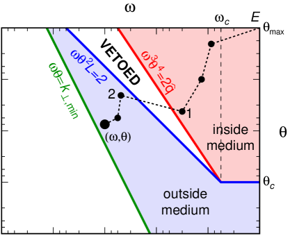
Figure 1: The phase-space for vacuum-like gluon emissions by a jet propagating through a dense QCD medium, in logarithmic units. In the left plot, the variables are the gluon energy $\omega$ and its emission angle $\theta$. In the right plot, we rather use the relative transverse momentum $k_{\perp}\simeq\omega\theta$ and the inverse of the angle $1/\theta$.

Eq. (3) is the cornerstone on which the partonic cascade in the medium is built. From this fundamental relation, the full physical picture can be obtained based on a few additional observations:

• The formation time $t_{\rm med}(\omega)$ corresponding to a MIE must be shorter than $L$, implying an upper limit on the energy of the MIEs: $\omega\leq\omega_{c}\equiv\hat{q}L^{2}/2$. This argument also shows that the constraint in Eq. (3) exists only for $\omega\leq\omega_{c}$; more energetic emissions with $\omega>\omega_{c}$ are always vacuum-like, irrespective of their formation time (smaller or larger than $L$).

• VLEs can either occur inside the medium, in which case they satisfy (3), or outside the medium, in which case $t_{\rm f}(\omega,\theta)>L$. This implies that emissions with intermediate formation times, with $t_{\text{med}}\ll t_{\text{f}}(\omega,\theta)\ll L$, are forbidden. This gives the “vetoed” region in Fig. 1.

• The above one-emission picture can be generalised to the multiple emission of $N$ gluons with $\omega_{n}\ll\omega_{n-1}$ and $\theta_{n}\ll\theta_{n-1}$, $n=1,\dots,N$. The corresponding formation times are strongly increasing from one emission to the next one, $t_{{\rm f},n}\gg t_{{\rm f},n-1}$ (with $t_{{\rm f},n}\equiv t_{\rm f}(\omega_{n},\theta_{n})$). As a consequence if Eq. (3) is satisfied by the last emitted gluon i.e. if $t_{{\rm f},N}\ll t_{\rm med}(\omega_{N})$, then it is automatically satisfied by all earlier emissions, $t_{{\rm f},n}\ll t_{\rm med}(\omega_{n})$.

• To obtain the strong ordering above we have assumed that emissions were both soft and collinear. This is known as the double-logarithmic approximation where the emission probability (2) is enhanced by logarithms of both the energy and the emission angle. This approximation is at the heart of a large range of calculations in perturbative QCD. We briefly discuss below some new elements (and limitations) going beyond this approximation in the next section.

• A key ingredient of the above generalisation to multiple gluon emissions is the fact that the in-medium partonic cascade preserves angular ordering, meaning that $\theta_{n}\ll\theta_{n-1}$. This is highly non-trivial as this is a subtle consequence of colour coherence for vacuum emissions and collisions in the medium which eventually wash out this coherence Caucal:2018dla .

• The characteristic time for colour decoherence is MehtarTani:2010ma ; MehtarTani:2011tz ; CasalderreySolana:2011rz ; MehtarTani:2011gf

  $$t_{\rm coh}(\theta)\,=\,\Big{(}\frac{4}{\hat{q}\theta^{2}}\Big{)}^{1/3}.$$ (4)

  Hence, VLEs with emission angles $\theta\gg\theta_{c}\equiv 2/\sqrt{\hat{q}L^{3}}$ rapidly lose their colour coherence ($t_{\rm coh}(\theta)\ll L$) and act as independent sources for MIEs over a time $\Delta t\simeq L$. Conversely, VLEs with $\theta<\theta_{c}$ remain coherent with their parent parton and are not discriminated by the medium: the associated pattern of MIEs is as if created by their parent. This explains why the emissions with $\theta<\theta_{c}$ are included in the “outside” region in Fig. 1.

• Over the development of a vacuum-like cascade, the partons can also lose energy by emitting MIEs. Since the (relative) energy loss is suppressed as $(t_{\rm f}(\omega,\theta)/t_{\rm med}(\omega))^{2}\ll 1$ this effect can be neglected. In other words, even though the partons created via VLEs will ultimately lose energy via MIEs, this effect is negligible during the development of the vacuum-like cascade. Note that Eq. (3) also means that broadening effects are negligible.

• After being emitted at a time $t$, a parton propagates through the medium over a distance $L-t$. During this propagation it interacts with the medium. From the point of view of these interactions with the medium, we can safely set the formation time of the VLEs to 0, as a consequence of the strong ordering in formation time. Therefore, MIEs and transverse momentum broadening can occur at any time $0<t<L$. We describe these phenomena in the following sections.

• Once the partons have travelled through the medium, undergoing MIEs and broadening, they are again allowed to fragment as a standard vacuum-like cascade outside the medium. Since the partons have lost their colour coherence during their traversal of the medium, the first emission in the outside-medium VLE cascade can violate angular ordering i.e. happen at any angle Caucal:2018dla .

A very simple picture for the development of a partonic cascade in the medium emerges from the above observations. The full cascade can be factorised in three major steps, represented in Fig. 1:

1. in-medium vacuum-like cascade: an angular-ordered vacuum-like cascade governed by the standard DGLAP splitting functions occurs inside the medium up to $t_{\rm f}(\omega,\theta)=t_{\rm med}(\omega)$. During this process, the only effect of the medium is to set the constraint (3) on the formation time;

2. medium-induced emissions and broadening: every parton resulting from the in-medium cascade travels through the medium, possible emitting (a cascade of) MIEs and acquiring momentum broadening (see discussions below for details);

3. outside-medium vacuum-like cascade: each parton exiting the medium at the end of the previous step initiates a new vacuum-like cascade outside the medium, down to a non-perturbative cut-off scale. The first emission in this cascade can happen at an arbitrary angle.

Before moving to new considerations specific to this paper, let us provide a few additional comments of use for our later discussions. First of all, the condition (3) can be reformulated as a lower limit on the emission angle $\theta$ for a given energy, $\theta\gg\theta_{0}(\omega)\equiv\left({2\hat{q}}/{\omega^{3}}\right)^{\!\frac{1}{4}}$, or as a condition on the energy of the emission at fixed angle $\theta$: $\omega>\omega_{0}(\theta)\equiv\left({2\hat{q}}/{\theta^{4}}\right)^{\!\frac{1}{3}}$. Physically, $\theta_{0}(\omega)$ is the formation angle of a MIE, i.e. the value of the emission angle at the time of formation.

Furthermore, one can easily compute the in-medium parton multiplicity at a given energy and angle in the above double-logarithmic approximation. Each emission is enhanced by a double logarithm and the corresponding contribution to the double differential gluon distribution at a given point $(\omega,\theta)$ in phase-space is, using a fixed-coupling approximation

$$\frac{{\rm d}^{2}N_{\rm DLA}^{\text{(in-medium)}}}{{\rm d}\omega{\rm d}\theta^{2}}=\,\frac{\bar{\alpha}_{s}}{\omega\,\theta^{2}}\sum_{n\geq 0}\,\bar{\alpha}_{s}^{n}\left[\frac{1}{n!}\ln^{n}\frac{E}{\omega}\right]\left[\frac{1}{n!}\ln^{n}\frac{\theta_{\rm max}^{2}}{\theta^{2}}\right]=\frac{\bar{\alpha}_{s}}{\omega\,\theta^{2}}\,{\rm I}_{0}\left(2\sqrt{\bar{\alpha}_{s}\ln\frac{E}{\omega}\,\ln\frac{\theta_{\rm max}^{2}}{\theta^{2}}}\right),$$ (5)

where $\bar{\alpha}_{s}=\tfrac{\alpha_{s}N_{c}}{\pi}$ and $\theta_{\text{max}}$ is the maximal angle allowed for the emissions. The term with $n=0$ in this series represents the direct emission of the gluon $(\omega,\theta)$ by the leading parton, while a term with $n\geq 1$ describes a sequence of $n$ intermediate emissions acting as additional sources for the final gluon.

Finally, note that whereas it provides a reasonable (first) estimate for the gluon multiplicity at small $\omega\ll E$, the above double-logarithmic approximation (DLA) proposed in Ref. Caucal:2018dla is not appropriate for observables which are sensitive to the energy loss, or for quantitative studies of the multiplicity. This is due to two main reasons: the DLA for the VLEs uses only the singular part of the splitting functions, i.e. $P(z)\simeq 2C_{R}/z$, and the energy of the parent parton is unmodified after the emission so the energy is not conserved at the splitting vertices. In the next section we show that this can easily be fixed by accounting for the full splitting function. Second, MIEs, which represent the main mechanism for jet energy loss in the medium, were neglected at DLA. However, the factorisation between VLEs and MIEs (described above) which was rigorously proven at DLA Caucal:2018dla is still valid beyond, typically in the single logarithmic approximation in which one only enforces a strong ordering of the successive emissions angles. One can therefore include MIEs and broadening effects in the above picture, as described in the text below. This is the picture that we adopt throughout this paper.

2.3 A single-logarithmic approximation with angular ordering

Now that we have recalled the basic picture for the development of parton showers in the presence of a medium, we show that several subleading corrections, beyond DLA, can easily be taken into account.

The validity of our factorisation between VLEs and MIEs relies on strong inequalities between the formation times. Clearly, these inequalities do still hold if the strong ordering refers only to the emission angles ($\theta_{n}\ll\theta_{n-1}$), but not also to the parton energies (as is the case beyond the soft limit $z\ll 1$). There is nevertheless some loss of accuracy w.r.t. a strict single logarithmic approximation associated with the uncertainties in the boundaries of the vetoed region in phase-space. Notably the condition $t_{\rm f}(\omega,\theta)=t_{\rm med}(\omega)$ defining the upper boundary is unambiguous only at DLA. For a generic splitting fraction $z$, the formation times also depend upon the energy $xE$ of the parent parton and not just upon the energy $\omega=xzE$ of the soft daughter gluon. For a generic $1\to 2$ splitting where the “vacuum-like” formation time $t_{\rm f}\equiv t_{\rm f}(x,z,\theta)$ is given by Eq. (1) with $E\to xE$. The corresponding “medium” formation time $t_{\rm med}(x,z)$ is different for different partonic channels. For example, for a $g\to gg$ splitting, it reads (see e.g. Blaizot:2012fh ; Blaizot:2013vha ; Apolinario:2014csa )

$$t_{\rm med}(x,z)\big{|}_{g\to gg}\,=\,\sqrt{\frac{2z(1-z)xE}{\hat{q}_{\text{eff}}(z)}}\ \overset{z\ll 1}{\approx}\ \sqrt{\frac{2\omega}{\hat{q}}}\,,\qquad\hat{q}_{\text{eff}}(z)\equiv\hat{q}\big{[}1-z(1-z)\big{]},$$ (6)

with $\omega=zxE$. One could in principle use these more accurate estimates for $t_{\rm f}$ and $t_{\rm med}$ in Eq. (3). One would then need to deal with the difficulty that the evolution phase-space depends explicitly on $xE$, $z$ and $\theta$ and not just on $\omega$ and $\theta$. The corresponding generalisation of Eq. (3) would also be different for different partonic channels. Last but not least, the distinction between VLEs and MIEs according to their formation times only holds so long as the strong inequality $t_{\rm f}\ll t_{\rm med}$ is satisfied, meaning that the precise form of the boundary could also be sensitive to subleading corrections. In practice, our strategy to deal with this ambiguity (notably, in the Monte-Carlo simulations) is to stick to the simpler form of the boundary in Eq. (3), but study the sensitivity of our results to variations in $\hat{q}$, effectively mimicking the $z$-dependence of $t_{\rm med}(x,z)$ in Eq. (6) when $z\sim\mathcal{O}{(1)}$. Similarly, the ambiguity in the definition of the other boundary of the “vetoed” region, which corresponds to $t_{\rm f}=L$, can be numerically studied by considering variations in $L$.

2.4 Medium-induced radiation

We now turn to a discussion of the medium-induced radiation and the associated energy loss. We start by observing that all the partons created via VLEs with emission angles $\theta\gg\theta_{c}$ act as quasi-independent sources for MIEs. Such partons have very short formation times, $t_{\rm f}(\omega,\theta)\ll L$, so after formation they propagate through the medium over a distance of the order of the medium size $L$. Since their coherence time $t_{\rm coh}(\theta)$ (cf. Eq. (4)) is much smaller that $L$, they rapidly lose colour coherence during this propagation. Each parton therefore acts as independent sources for medium-induced radiation with energies up to $\omega_{c}=\hat{q}L^{2}/2$ (such that $t_{\rm med}(\omega_{c})=L$).

In practice, the emissions which control the energy loss by the jet , i.e. emissions at large angles, are dominated by much softer gluons, with energies $\omega\ll\omega_{c}$ and short formation times $t_{\rm med}(\omega)\ll L$ Blaizot:2013hx ; Fister:2014zxa . Since these soft emissions occur with a probability of order one, one must include multiple branching to all orders. With this kinematics, this multiple-branching problem can be treated as a classical Markovian process CasalderreySolana:2011rz ; Blaizot:2012fh ; Blaizot:2013hx ; Blaizot:2013vha ; Apolinario:2014csa ; Arnold:2015qya ; Arnold:2016kek . This stems from the following two observations: (i) the time interval between two MIEs of comparable energies is much larger than their respective formation time, meaning hat successive MIEs do not overlap with each other, and (ii) interference effects can be neglected since, in a medium-induced branching, the colour coherence between the daughter partons is lost during formation. This last point also implies that successive MIEs do not obey angular ordering. The evolution “time” of the Markovian process is the physical time $t$ at which the MIEs occur in the medium (with $0<t<L$).

The differential probability for one emission is given by the BDMPS-Z spectrum for energies $\omega\ll\omega_{c}$ Baier:1996kr ; Baier:1996sk ; Zakharov:1996fv ; Zakharov:1997uu ; Baier:1998kq (see also Wiedemann:2000za ; Wiedemann:2000tf ; Arnold:2001ba ; Arnold:2001ms ; Arnold:2002ja for related developments). For definiteness, consider the $g\to gg$ splitting of a gluon of energy $xE$ (see e.g. Mehtar-Tani:2018zba for the other partonic channels). The differential splitting rate integrated over the emission angles (or, equivalently, over the transverse momentum $\bm{k}_{\perp}$) reads

$$\frac{{\rm d}^{2}\Gamma_{\rm med}}{{\rm d}z{\rm d}t}=\frac{\alpha_{s}P_{g\to gg}(z)}{2\pi}\sqrt{\frac{\hat{q}_{\text{eff}}(z)}{z(1-z)xE}}=\frac{\alpha_{s}P_{g\to gg}(z)}{\sqrt{2}\pi}\frac{1}{t_{\rm med}(x,z)}$$ (7)

where it is understood that $z(1-z)xE\ll\omega_{c}$. The second rewriting above uses Eq. (6) and makes it clear that the splitting rate is proportional to the inverse formation time.

It is interesting to consider the emission probability (integrated over a time/distance $L$), i.e. the BDMPS-Z spectrum for a single soft emission, in the limit of a soft splitting, $z\ll 1$. We find

$$\omega\frac{{\rm d}\mathcal{P}_{\rm med}}{{\rm d}\omega}=\bar{\alpha}_{s}\sqrt{\frac{2\omega_{c}}{\omega}}\,\Theta(\omega_{c}-\omega),$$ (8)

where we have used $P_{g\to gg}(z)\simeq 2N_{c}/z$, $\bar{\alpha}_{s}=\alpha_{s}N_{c}/\pi$, $\omega=zxE$, and $\omega_{c}=\hat{q}L^{2}/2$.

So long as its r.h.s. is strictly smaller than one, Eq. (8) expresses the probability to emit a gluon with energy $\omega$ by an energetic gluon propagating through the medium along a distance $L$. For $\omega\sim\omega_{c}$, this probability is of $\mathcal{O}{(\bar{\alpha}_{s})}$, showing that hard MIEs are rare. On the contrary, the emission probability becomes of $\mathcal{O}{(1)}$ when $\omega\sim\omega_{\rm br}\equiv\bar{\alpha}_{s}^{2}\omega_{\rm c}$ at which point multiple branchings become important and the single-emission spectrum (8) is no longer appropriate.

For gluons with $\omega\lesssim\omega_{\text{br}}$, we can use (7) to estimate the typical time interval between successive branchings. It is given by the condition

$$\omega\frac{{\rm d}^{2}\Gamma_{\rm med}}{{\rm d}\omega{\rm d}t}\,t_{\rm br}(\omega)\,\sim\,1\qquad\Longrightarrow\qquad t_{\rm br}(\omega)\,\simeq\,\frac{1}{\bar{\alpha}_{s}}\,t_{\rm med}(\omega)\,.$$ (9)

The fact that this is parametrically larger than the formation time $t_{\rm med}(\omega)$ justifies the picture of independent emissions. Note that $t_{\rm br}(\omega)<L$ when $\omega<\omega_{\rm br}$.

The hard but rare emissions with $\omega\sim\omega_{c}$ control the average energy lost by the leading parton, as can be seen by integrating Eq. (8) over $\omega$: the integral is dominated by its upper limit $\omega_{c}$ and yields, parametrically, $\varepsilon_{\rm LP}\sim\bar{\alpha}_{s}\omega_{c}$. However, a hard emission with $\omega\sim\omega_{c}$ makes a small angle $\theta\sim\theta_{c}\ll R$ w.r.t. the jet axis and hence remains inside the jet. To estimate the energy lost by the jet, one must instead consider the emissions which are soft enough to be deviated outside the jet via elastic collisions. For this, we need a more quantitative understanding of the transverse momentum broadening.

2.5 Transverse momentum broadening

We first consider a MIE with $\omega_{\rm br}\ll\omega\ll\omega_{\rm c}$, i.e. soft but not too soft, emitted at a time $t$. In this case, multiple emissions can be neglected and after being emitted, the gluon propagates through the medium over a distance $L-t$. Via elastic collisions, this gluon accumulates a transverse momentum $k_{\rm f}^{2}\simeq\hat{q}t_{\rm f}$ during its formation and an additional $\Delta k_{\perp}^{2}=\hat{q}(L-t)$ after formation. Given that $t_{\rm f}\ll L$ and $L-t\sim L$, we have $k_{\rm f}^{2}\ll\Delta k_{\perp}^{2}$. We can therefore neglect the momentum broadening during formation and assume that the MIE is produced collinearly with its source. Accordingly, the final transverse momentum distribution of this gluon can be approximated by

$$\frac{{\rm d}\mathcal{P}_{\rm broad}}{{\rm d}^{2}\bm{k}_{\perp}}=\,\frac{1}{\pi\hat{q}(L-t)}\exp\left\{-\frac{k_{\perp}^{2}}{\hat{q}(L-t)}\right\}\,.$$ (10)

The maximal average transverse momentum that can be acquired in this way is $Q_{s}^{2}\equiv\hat{q}L$ (realised for $t=0$). Using $k_{\perp}\simeq\omega\theta$ and averaging over the azimuthal angle one can rewrite (10) as

$$\frac{{\rm d}\mathcal{P}_{\rm broad}}{{\rm d}\theta}\simeq\frac{2\omega^{2}\theta}{\hat{q}(L-t)}\exp\left\{-\frac{\omega^{2}\theta^{2}}{\hat{q}(L-t)}\right\}.$$ (11)

This strictly applies to soft emitted gluons ($\omega\ll\omega_{\rm c}$) and small angles ($\theta\ll 1$), but it is formally normalised by integrating over all values $0<\theta<\infty$. The above equations describe the Gaussian broadening via multiple soft scattering, but neglect the possibility to acquire large transverse momentum $k_{\perp}^{2}\gg\hat{q}(L-t)$ via a single hard scattering.

We now move to even softer MIEs with energies $\omega\lesssim\omega_{\rm br}$ which have a finite lifetime $t_{\rm br}(\omega)<L$ (and much shorter formation times $t_{\rm f}\ll t_{\rm br}$, cf. Eq. (9)). The momentum/angular broadening is therefore obtained by replacing $L-t\to t_{\rm br}(\omega)$ in Eqs. (10)–(11) yielding a typical deviation angle

$$\theta(\omega)\simeq\frac{\sqrt{\hat{q}t_{\rm br}(\omega)}}{\omega}=\frac{1}{\sqrt{\bar{\alpha}_{s}}}\left(\frac{2\hat{q}}{\omega^{3}}\right)^{1/4}\gtrsim\theta(\omega_{\rm br})\simeq\frac{\theta_{c}}{\bar{\alpha}_{s}^{2}}\,,$$ (12)

This angle is large and typically larger than the jet opening angle $R$. Furthermore, gluons with energies $\omega\lesssim\omega_{\rm br}$ have a probability of $\mathcal{O}{(1)}$ to undergo a democratic branching. They therefore split over and over again in many soft quanta at large angles until they thermalise in the plasma via elastic collisions Iancu:2015uja . This implies in particular that the whole energy carried by primary emissions with $\omega\lesssim\omega_{\rm br}$ is eventually lost by the jet. (See also the next subsection.)

2.6 Energy loss by the jet: medium-induced emissions only

So far, we have argued that the energy lost by the jet via medium-induced radiation at large angles ($\theta>R$) is controlled by multiple branchings (resummed to all orders) and the associated characteristic scale is $\omega_{\rm br}=\bar{\alpha}_{s}^{2}\hat{q}L^{2}/2$. To facilitate the physical interpretation of our subsequent Mote-Carlo results it is useful to first recall a few more specific analytic results related to energy loss Blaizot:2013hx ; Fister:2014zxa ; Blaizot:2014ula ; Blaizot:2014rla ; Escobedo:2016jbm ; Escobedo:2016vba .

These previous studies only addressed the case of jets generated via medium-induced emissions alone, and with a simplified version of the BDMPS-Z kernel where only the poles at $z=0$ and $z=1$ in the splitting rate from Eq. (7) were kept. This is indeed sufficient to capture the most salient features of the full dynamics while allowing for a good degree of physical insight.

First, it has been shown Blaizot:2013hx that for a leading parton of energy $E<\omega_{c}$, the energy lost by a jet via multiple soft branchings at large angles is given by (with $\upsilon_{0}=2\pi$)

$$\varepsilon_{\rm flow}(E)\,=\,E\big{(}1-{\rm e}^{-\upsilon_{0}\frac{\omega_{\rm br}}{E}}\big{)}.$$ (13)

This contribution is independent of the jet radius $R$.

To this “turbulent” component of the jet energy loss, one must add the (average) energy taken away by semi-hard gluons whose energies are larger than $\omega_{\text{br}}$, yet small enough for the associated propagation angles $\theta\sim Q_{s}/\omega$ to be larger than $R$. The (average) semi-hard contribution to the energy loss is therefore obtained by integrating the emission spectrum over $\omega$ up to $\bar{\omega}\equiv c_{*}Q_{s}/R$, with $c_{*}$ a number smaller than one:

$$\varepsilon_{\rm spec}(E,R)\,\simeq\int_{0}^{\bar{\omega}}{\rm d}\omega\,\bar{\alpha}_{s}\sqrt{\frac{2\omega_{c}}{\omega}}\,{\rm e}^{-\upsilon_{0}\frac{\omega_{\rm br}}{E}}\,=\,2\bar{\alpha}_{s}\omega_{\rm c}\sqrt{\frac{2c_{*}\theta_{c}}{R}}\,{\rm e}^{-\upsilon_{0}\frac{\omega_{\rm br}}{E}}\,,$$ (14)

where we have also used $Q_{s}=\theta_{c}\omega_{\rm c}$. Note that the above expression uses the BDMPS-Z spectrum dressed by multiple branchings computed under the same assumptions as Eq. (13) yielding an extra exponential factor Blaizot:2013hx . The $R$-dependence here is easy to understand: with increasing $R$, more and more semi-hard emissions are captured inside the jet so the energy loss is decreasing. Not that when $R$ becomes as small as $\theta_{c}$, all the MIEs are leaving the jet and the average energy loss by the jet coincides with that of the leading parton. In practice, one usually has $R\gg\theta_{c}$ and therefore $\varepsilon_{\rm spec}\ll\varepsilon_{\rm LP}$.

The total energy lost by the jet under the present assumptions is $\varepsilon_{\text{MIE}}=\varepsilon_{\rm flow}+\varepsilon_{\rm spec}$, where the subscript “MIE” indicates that for the time being only MIEs are included. Eqs. (13)–(14) exhibit some general features which go beyond the approximations required for their derivation (see Blaizot:2013hx ; Fister:2014zxa ):

• For jets with energies $E\gg\upsilon\omega_{\rm br}$, the jet energy loss via MIEs becomes independent of $E$:

  $$\varepsilon_{\text{MIE}}(R)\,\simeq\,\upsilon\omega_{\rm br}+2\bar{\alpha}_{s}\omega_{\rm c}\sqrt{\frac{2c_{*}\theta_{c}}{R}}\qquad\mbox{when}\quad E\gg\upsilon\omega_{\rm br}\,.$$ (15)

  The parameter $\upsilon$, equal to $\upsilon_{0}=2\pi$ for the simplified branching kernel considered in Blaizot:2013hx , is smaller for the full splitting rate: for jets with $E<\omega_{\rm c}$, one finds $\upsilon\simeq 4.96$ Baier:2000sb ; Blaizot:2013hx , whereas in the high-energy limit $E\gg\omega_{\rm c}$, Ref. Fister:2014zxa reported $\upsilon\simeq 3.8$ for $\bar{\alpha}_{s}=0.25$.

• Jets with $E\lesssim\upsilon\omega_{\rm br}$ lose their whole energy via democratic branchings: $\varepsilon_{\text{MIE}}\simeq\varepsilon_{\rm flow}\simeq E$.

• For a large jet radius $R\gtrsim\theta_{c}/\bar{\alpha}_{s}^{2}$, the flow component dominates over the spectrum component, $\varepsilon_{\rm flow}\gg\varepsilon_{\rm spec}$, for any energy $E$, and the energy loss $\varepsilon_{\text{MIE}}\simeq\varepsilon_{\rm flow}$ becomes independent of $R$.

2.7 Energy loss by the jet: full parton shower

We can now consider the generalisation of the above results to the full parton showers, including both VLEs and MIEs. In our sequential picture, in which the two kind of emissions are factorised in time, each of the VLE inside the medium act as an independent source of MIEs and hence the energy loss by the full jet can be computed by convoluting the distribution of partonic sources created by the VLEs in the medium with the energy loss via MIEs by any of these sources. Assuming that all the in-medium VLEs are collinear with the jet axis (which is the case in the collinear picture described in Sect. 2.2), the energy lost by the full jet is computed as

$$\mathcal{E}_{\rm{jet}}(E,R) \simeq\int_{\omega_{0}(R)}^{E}{\rm d}\omega\,\frac{{\rm d}N_{\text{VLE}}}{{\rm d}\omega}\,\varepsilon_{\text{MIE}}(\omega,R)\,,$$

$$\simeq\varepsilon_{\text{MIE}}(E,R)+2\bar{\alpha}_{s}\int_{\theta_{c}}^{R}\frac{{\rm d}\theta}{\theta}\int_{\omega_{0}(\theta)}^{E}\frac{{\rm d}\omega}{\omega}\,{\rm I}_{0}\left(2\sqrt{\bar{\alpha}_{s}\ln\frac{E}{\omega}\,\ln\frac{R^{2}}{\theta^{2}}}\right)\varepsilon_{\text{MIE}}(\omega,R)\,,$$ (16)

where ${{\rm d}N_{\text{VLE}}}/{{\rm d}\omega}$ is the energy distribution of the partons created via VLEs inside the medium (cf. Fig. 1). The second line follows after using the DLA result for the gluon multiplicity, Eq. (5). This is of course a rough approximation which overestimates the number of sources, but it remains useful to get a physical insight. Similarly, for qualitative purposes, one can use the simple estimate for $\varepsilon_{\text{MIE}}(\omega,R)$ given by the sum of Eqs. (13)–(14).

3 Parton shower in the medium: Monte-Carlo implementation

The factorised picture for parton showers in the medium developed in the last section (see in particular Sect. 2.2), is well-suited for an implementation as a Monte Carlo generator. In this section we describe the main lines of this implementation and its limitations. We also provide the details for the simulations done throughout this paper.

Generic kinematic.

We will represent the massless 4-vectors corresponding to emissions using their transverse momentum $p_{Ti}$, their rapidity $y_{i}$ and their azimuth $\phi_{i}$. Since our physical picture is valid in the collinear limit, we will often neglect differences between physical emission angles $\theta$ and distances $\Delta R=\sqrt{\Delta y^{2}+\Delta\phi^{2}}$ in the rapidity-azimuth plane. All showers are considered to be initiated by a single parton of given transverse momentum $p_{T0}$, rapidity $y_{0}$ and azimuth $\phi_{0}$, and of a given flavour (quark or gluon).

Vacuum shower.

Still working in the collinear limit we will generate our partonic cascades using an angular-ordered approach, starting from an initial opening angle $\theta_{\text{max}}$. The initial parton can thus be seen as having $\theta=\theta_{\text{max}}$ and a relative transverse momentum $k_{\perp}=p_{T0}\theta_{\text{max}}$. To regulate the soft divergence of the splitting functions, we introduce a minimal (relative) transverse momentum cut-off $k_{\perp,\text{min}}$. This corresponds to the transition towards the non-perturbative physics of hadronisation (see Fig. 1). Note that for a particle of transverse momentum $p_{T}$, the condition $k_{\perp}>k_{\perp,\text{min}}$ imposes a minimal angle for the next emission: $\theta>\theta_{\text{min}}=k_{\perp,\text{min}}/p_{T}$.

The shower is generated using the Sudakov veto algorithm. More precisely, if the previous emission happened at an angle $\theta_{0}$ and with relative transverse momentum $k_{\perp 0}$ (i.e. with transverse momentum $p_{T0}=k_{\perp 0}/\theta_{0}$), the next emission is generated with coordinates $\theta$, $k_{\perp}$ (and hence with $p_{T}=k_{\perp}/\theta$), using the following procedure. We first generate the angle $\theta$ according to the Sudakov factor

$$\Delta_{i}(\theta|\theta_{0},k_{\perp 0}) =\exp\bigg{[}-\int_{\theta}^{\theta_{0}}\frac{{\rm d}\theta^{\prime}}{\theta^{\prime}}\int_{k_{\perp,\text{min}}}^{k_{\perp 0}}\frac{{\rm d}k_{\perp}^{\prime}}{k_{\perp}^{\prime}}\frac{2\alpha_{s}(k_{\perp}^{\prime})C_{i}}{\pi}\bigg{]}$$ (17)

$$=\exp\bigg{[}-\frac{C_{i}}{\pi\beta_{0}}\log\Big{(}\frac{1-2\alpha_{s}\beta_{0}\log(k_{\perp 0}/M_{Z})}{1-2\alpha_{s}\beta_{0}\log(k_{\perp,\text{min}}/M_{Z})}\Big{)}\log\Big{(}\frac{\theta_{0}}{\theta}\Big{)}\bigg{]},$$ (18)

where $i=(\text{g,\,q})$ is a flavour index, $C_{\text{g}}\equiv C_{A}$, $C_{\text{q}}\equiv C_{F}$, and we use 5 flavours of massless quarks. To obtain the second line, we used a 1-loop running coupling $\alpha_{s}(k_{\perp})=\tfrac{\alpha_{s}}{1-2\alpha_{s}\beta_{0}\log(k_{\perp}/M_{Z})}$ with $\alpha_{s}\equiv\alpha_{s}(M_{Z})$ the running coupling at the $Z$ mass, fixed to 0.1265, and $\beta_{0}=(11C_{A}-2n_{f})/(12\pi)$ the 1-loop QCD $\beta$ function (with $n_{f}=5$). The $k_{\perp}$ of the emission is then generated between $k_{\perp,\text{min}}$ and $k_{\perp 0}$ following the distribution $\tfrac{{\rm d}k_{\perp}}{k_{\perp}}\alpha_{s}(k_{\perp})$. This procedure neglects finite effects in the splitting function and momentum conservation as the splitting fraction $z^{\prime}\equiv\tfrac{p_{T}^{\prime}}{p_{T0}}=\tfrac{k_{\perp}^{\prime}}{k_{\perp 0}}\tfrac{\theta_{0}}{\theta^{\prime}}$ associated with the emission of the gluon $\theta^{\prime}$ and $k_{\perp}^{\prime}$ in (17) can take values larger than one. This is simply taken into account by vetoing emissions with $z>1$ and accepting those with $z\leq 1$ with a probability $\tfrac{z}{2C_{i}}P_{i}(z)$ with $P_{i}(z)$ the targeted splitting function. If any of these vetoes fails, we set $\theta\to\theta_{0}$ and $k_{\perp}\to k_{\perp 0}$ and reiterate the procedure. After a successful parton branching, both daughter partons are further showered. The procedure stops when the generated angle $\theta$ is smaller than the minimal angle $\theta_{\text{min}}$.

To fully specify the procedure we still need to specify how to reconstruct the daughter partons from the parent. For this, we use $z\equiv\tfrac{p_{T}}{p_{T0}}=\tfrac{k_{\perp}}{k_{\perp 0}}\tfrac{\theta_{0}}{\theta}$ and also generate an azimuthal angle $\varphi$ around the parent parton, randomly chosen between 0 and $2\pi$. We then write

$$\text{parent: }(p_{T0},y_{0},\phi_{0})\longrightarrow\begin{cases}\text{daughter 1: }\big{(}z\,p_{T0},y_{0}+(1-z)\theta\cos(\varphi),\phi_{0}+(1-z)\theta\sin(\varphi)\big{)}\\ \text{daughter 2: }\big{(}(1-z)p_{T0},y_{0}-z\,\theta\cos(\varphi),\phi_{0}-z\,\theta\sin(\varphi)\big{)}\end{cases}.$$ (19)

Medium shower: MIEs.

The cascade of MIEs is better described using an ordering in emission time. For simplicity, we assume a uniform medium of fixed length $L$ and adopt a fixed-coupling approximation for the interactions between the hard partons and the medium, with no feedback.

The rate for the emission of a MIE per unit time is given by the kernel (see e.g. Blaizot:2013vha )

$$\mathcal{K}(z|p_{T})\equiv\frac{\alpha_{s}}{2\pi}\sqrt{\frac{\hat{q}[1-z(1-z)]}{z(1-z)p_{T}}}P_{gg}(z)\overset{z\ll 1}{\approx}\frac{\alpha_{s}C_{A}}{\pi}\sqrt{\frac{\hat{q}}{p_{T}}}\frac{1}{[z(1-z)]^{3/2}},$$ (20)

where $p_{T}$ is the transverse momentum of the parton that splits and $z$ the splitting fraction. Throughout this paper, the QCD coupling occurring in Eq. (20) will be assumed to be fixed and treated as a free parameter, to be often denoted as ${\alpha}_{s,\text{med}}$ for more clarity. This Markovian process can be simulated from $t=0$ to $t=L$ using a Sudakov veto algorithm as for the vacuum-like shower. From a time $t_{0}$, we first generate the next splitting time $t$ according to a Sudakov factor which integrates (20) over time between $t_{0}$ and $t$ and over $z$ between some cut-off $z_{\text{min}}$ and $1-z_{\text{min}}$. We then generate $z$ according to (20). Both steps are done using the simplified kernel in the limit $z\ll 1$ and a veto with probability $\tfrac{z}{2C_{A}}P_{gg}(z)$ is applied to get the full splitting rate. In practice, we have set $z_{\text{min}}=10^{-5}$ and checked that this choice has no influence on our final results.

In the cascade described above, all the splittings are considered to be exactly collinear. The angular pattern is generated afterwards via transverse momentum broadening, cf. Sect. 2.5. For this, we go over the whole cascade and, for each parton, we generate an opening angle $\theta$ and azimuthal angle $\varphi$ according to the two-dimensional Gaussian distribution Eq. (11) where $L-t$ is replaced by the lifetime $\Delta t$ of the parton in the cascade. Once we have the transverse momenta and angles of each parton in the cascade, we use (19) to reconstruct the kinematics. Partons which acquire an angle larger than $\theta_{\text{max}}$ via broadening are discarded together with their descendants.

Medium shower: global picture.

The in-medium shower is generated in three stages, according to the factorisation discussed in Sect. 2.2. The first step is to generate in-medium VLEs. This is done exactly as for the full vacuum shower except that each emission is further tested for the in-medium conditions $k_{\perp}^{3}\theta>2\hat{q}$ and $\theta>\theta_{c}$. If any of these two conditions fails, the emission is vetoed. The second step is to generate MIEs for each of the partons obtained at the end of the first step, following the procedure described above. The third step is to generate the VLEs outside the medium. For this, each parton at the end of the MIE cascade is taken and showered outside the medium. This uses again the vacuum shower, starting from an angle $\theta_{\text{max}}$ since decoherence washes out angular ordering for the first emission outside the medium. Each emission which satisfies either $k_{\perp}\theta<2/L$ or $\theta<\theta_{c}$ is kept, the others are vetoed.

Final-state reconstruction.

The full parton shower can be converted to 4-vectors suited for any analysis. Final-state (undecayed) partons are taken massless with a kinematics taken straightforwardly from Eq. (19). If needed, the 4-vectors of the other partons in the shower are obtained by adding the 4-momenta of their daughter partons. This requires traversing the full shower backwards.

Whenever an observable requires to cluster the particles into jets and manipulate them, we use the FastJet program (v3.3.2) Cacciari:2011ma and the tools in fjcontrib. In particular, the initial jet clustering is always done using the anti-$k_{\perp}$ algorithm Cacciari:2008gp with $R=0.4$ unless explicitly mentioned otherwise.

Limitations.

The Monte Carlo generator that is described above is of course very simplistic and has a series of limitations. We list them here for the sake of completeness. First of all, we only generate a partonic cascade, neglecting non-perturbative effects like hadronisation. Even if one can hope that these effects are limited — especially at large $p_{T}$ —, our description remains incomplete and, for example, track-based observables are not easily described in our current framework. Additionally, our partonic cascade only includes final-state radiation. Including initial-state radiation goes beyond our collinear picture and is left for future work. This would be needed, for example, to describe the transverse momentum pattern of jets recoiling against a high-energy photon.

Our description of the medium is also simplified: several effects like medium expansion, density non-uniformities and fluctuations, and the medium geometry are neglected. For the observables discussed in this paper, this can to a large extend be hidden into an adjustment of the few parameters we have left, but we would have to include all these effects to claim a full in-medium generator.

	parameters			physics constants
Description	$\hat{q}$ [GeV2/fm]	$L$ [fm]	${\alpha}_{s,\text{med}}$	$\theta_{c}$	$\omega_{c}$ [GeV]	$\omega_{\text{br}}$ [GeV]
default	1.5	4	0.24	0.0408	60	3.456
	1.5	3	0.35	0.0629	33.75	4.134
similar $R_{AA}$	2	3	0.29	0.0544	45	3.784
	2	4	0.2	0.0354	80	3.200
vary $\theta_{c}$	0.667	6	0.24	0.0333	60	3.456
	3.375	2.667	0.24	0.05	60	3.456
vary $\omega_{c}$	0.444	6	0.294	0.0408	40	3.456
	5.063	2.667	0.196	0.0408	90	3.456
vary $\omega_{\text{br}}$	1.5	4	0.196	0.0408	60	2.304
	1.5	4	0.294	0.0408	60	5.184

Table 1: Table of medium parameters used in this paper. The default set of parameters is given in the first line. The next 3 lines are parameters which give a similar prediction for $R_{\text{AA}}$. The last 6 lines are up and down variations of $\theta_{c}^{2}$, $\omega_{c}$ and $\omega_{\text{br}}$ by 50%, keeping the other two physics constants fixed.

Choices of parameters.

The implementation of in-medium partonic cascades described above has 5 free parameters: two unphysical ones, $\theta_{\text{max}}$ and $k_{\perp,\text{min}}$, essentially regulating the soft and collinear divergences, and three physical parameters, $\hat{q}$, $L$ and ${\alpha}_{s,\text{med}}$, describing the medium. In our phenomenological studies, we will make sure that our results are not affected by variations of the unphysical parameters and we will study their sensitivity to variations of the medium parameters.

The different sets of parameters we have used are listed in Table 1. The first line is our default setup. It has been chosen to give a reasonable description of the $R_{AA}$ ratio measured by the ATLAS collaboration (see Sect. 4.2 below). The next 3 sets are variants which give a similarly good description of $R_{AA}$ and can thus be used to test if other observables bring an additional sensitivity to the medium parameters compared to $R_{AA}$. The last 6 lines are variations that will be used to probe which physical scales, amongst $\theta_{c}$, $\omega_{c}$ and $\omega_{\text{br}}$, influence a given observable.

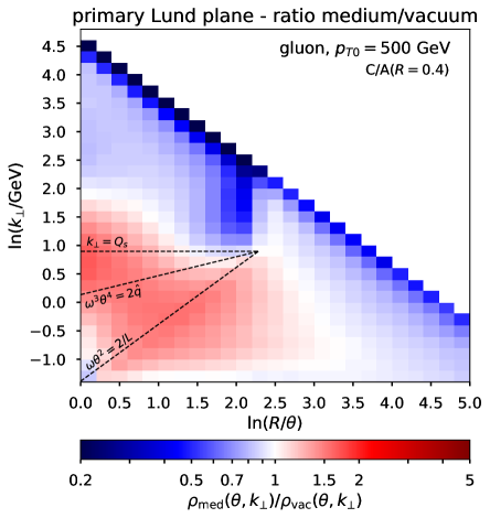
Figure 2: plot of the primary Lund plane density $\rho$ for the two main showers in our Monte Carlo: the vacuum shower (left) and the medium-induced shower (right). In both cases, the shower is initiated by a 500 GeV gluon.

Figure 3: Effect of the medium on the primary Lund plane density $\rho$. The left plot show the ratio of the density obtained with VLEs, taking into account the kinematic constraints from the medium, to the vacuum reference. The right plot is the ratio of the full shower over the vacuum density.

Illustration of the behaviour.

To illustrate the properties of our in-medium parton shower, we consider the primary Lund plane density $\rho(\theta,k_{\perp})$. In a nutshell, this uses an iterative declustering procedure, following the hardest branch at each step, to measure the density of emissions at an angle $\theta$ and with relative transverse momentum $k_{\perp}$ from the hard subjet (see Ref. Dreyer:2018nbf ). It can be viewed as a representation of the emissions from the leading parton in a jet.

Fig. 2 shows the primary Lund plane for the two main showers introduced above: the (genuine) vacuum-shower (left) — our reference for the calibration of the nuclear effects — and the medium-induced shower (right). The vacuum shower shows the expected pattern of a density which is mostly constant at a fixed $k_{\perp}$, increases due to the running of the strong coupling with decreasing $k_{\perp}$, and vanishes when approaching the kinematic limit $z\to 1$. The right plot of Fig. 2 highlights that MIEs have a typical transverse momentum $k_{\perp}\lesssim Q_{s}$ (cf. (10)) and a density which increases at small $z$.

Fig. 3 then shows the effect of our factorised picture for the parton shower in a dense plasma. In the left plot, we have neglected MIEs and only included the VLEs both inside and outside the medium. The plot shows the ratio of the resulting density to the vacuum density. The vetoed region is clearly visible on the plot. The small density reduction in the in-medium region and the small increase in the outside region, especially at large angles, can both be attributed to the fact that the first emission outside the medium can violate angular ordering and be emitted at any angle.

Finally, the right plot of Fig. 3 shows the ratio of the density $\rho_{\text{med}}$ for the full shower to the corresponding vacuum density. In this case, one clearly see a region of enhanced emissions corresponding to MIEs, as well as a decrease at large $p_{T}$ due to energy loss.

4 Energy loss by the jet and the nuclear modification factor

Here we present our Monte Carlo results for the jet nuclear modification factor $R_{AA}$. We first discuss the case of a monochromatic leading parton, for which we compute the jet energy loss, and then turn to $R_{AA}$ itself, using a Born-level jet spectrum for the hard process producing the leading parton.

4.1 The average energy loss by the jet

To study the jet energy loss we start with a single hard parton of transverse momentum $p_{T0}$ and shower it with the Monte Carlo including either MIEs only, or both VLEs and MIEs. The jet energy loss is defined as the difference between the energy of the initial parton and the energy of the reconstructed jet. To avoid artificial effects related to emissions with an angle $\theta$ between the jet radius $R$ and the maximal opening angle $\theta_{\text{max}}$ of the Monte Carlo, we have set $\theta_{\text{max}}=R$. Furthermore, for the case where both VLEs and MIEs are included, we have subtracted the pure-vacuum contribution (which comes from clustering and other edge effects and is anyway small for $\theta_{\text{max}}=R$).

Our results for the energy loss are shown in Fig 4 as a function of $E\equiv p_{T0}$ and in Fig. 5 as a function of $R$, for both gluon- and quark-initiated jets. For these plots we have used the default values for the medium parameters (see the first line of Table 1). Overall, we see a good qualitative agreement with the features expected from the theoretical discussion in sections 2.6 and 2.7.

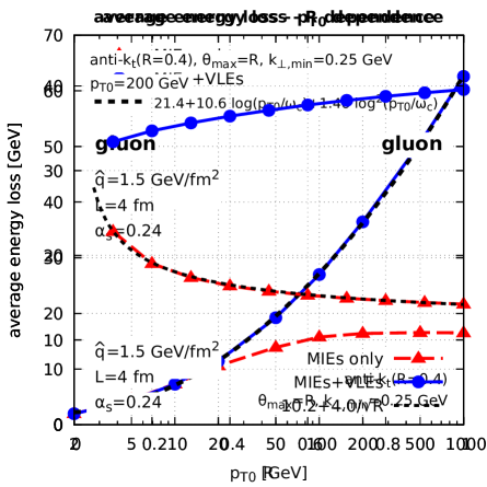
Figure 4: The MC results for the average energy loss by a gluon-initiate jet (left), respectively, a quark-initiated one (right), is displayed as a function of the initial energy $p_{T0}$ of the leading parton, for two scenarios for the jet evolution: jets with MIEs only (triangles) and full showers with both MIEs and VLEs (circles). The dashed line shows the quadratic fit to the energy loss by the full parton shower.

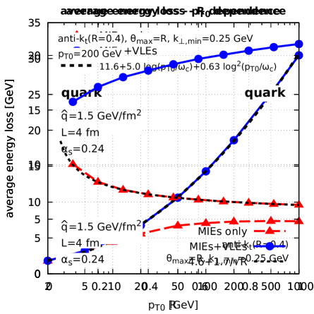
Figure 5: The MC results for the average energy loss by the jet are displayed as a function of the jet angular opening $R$, for the same choices as in Fig. 4. We also show in dashed line a fit (inspired by the theoretical estimate in Eq. (14)) for the jet built with MIEs alone.

For the jets involving MIEs only, we see that the energy loss first increases with $p_{T0}$ and then saturates, as predicted by Eqs. (13)–(14). Also, as a function of $R$ for fixed $p_{T0}=200$ GeV, it decreases according to the expected $1/\sqrt{R}$ behaviour, cf. Eq. (14). The agreement is even quantitatively decent. Indeed, with the physical parameters given in Table 1, the fitted $R$-dependence for gluon-initiated jets, $\varepsilon_{\text{MIE}}(R)\simeq\epsilon_{0}+\epsilon_{1}/\sqrt{R}$, with $\epsilon_{0}=10.2$ GeV and $\epsilon_{1}=4.0$ GeV, corresponds to the prediction in Eq. (15) provided one chooses $\upsilon\simeq 2.95$ and $c_{*}\simeq 0.38$, which are both reasonable.

Consider now the full parton showers, with both VLEs and MIEs. Although we do not have accurate-enough analytic results to compare with (only the DLA estimate Eq. (2.7)), the curves “MI+VLEs” in Figs. 4 and 5 show the expected trend: the energy loss increases with both $p_{T0}$ and $R$, due to the rise in the phase-space for VLEs. For later use, we have fitted the dependence on $p_{T0}$ with a quadratic polynomial in $\ln(p_{T0}/\omega_{c})$ and the resulting coefficients are shown on Fig. 4.

It is also striking from Figs. 4 and 5, that the average energy loss obeys a surprisingly good scaling with the Casimir colour factor of the leading parton: the energy loss by the quark jet is to a good approximation equal to $C_{F}/C_{A}=4/9$ times the energy loss by the gluon jet. Such a scaling, natural in the case of a single-gluon emission, is very non-trivial in the presence of multiple branchings. Let us first give an argument explaining this scaling for the case of MIEs alone. The main observation (see Blaizot:2013hx ; Fister:2014zxa ; Mehtar-Tani:2018zba for more details and for numerical results) is that the small-$x$ gluon distribution within a jet initiated by a parton of colour representation $R$ develops a scaling behaviour with $1/x$, known as a Kolmogorov-Zakharov (or “turbulent”) fixed point. For large-enough initial jet energy $E\equiv p_{T0}$ this scaling spectrum is identical to the BDMPS-Z spectrum created by a single emission and reads

$$x\frac{{\rm d}G_{R}}{{\rm d}x}\,\simeq\,\frac{\alpha_{s}C_{R}}{\pi}\sqrt{\frac{\hat{q}L^{2}}{xE}}\qquad\mbox{for \ $x\ll 1$ \ and}\ \ E\gg\omega_{\rm br}^{(R)}\equiv\frac{\alpha_{s}^{2}}{\pi^{2}}\,C_{A}C_{R}\,\frac{\hat{q}L^{2}}{2}\,,$$ (21)

where $\hat{q}$ is the gluonic jet quenching parameter, proportional to $C_{A}$, since Eq. (21) refers to the emission of soft gluons. This spectrum is directly proportional to the Casimir $C_{R}$ of the leading parton as expected. Note that the scale $\omega_{\rm br}^{(R)}$ which appears in the validity condition of Eq. (21) involves the product $C_{A}C_{R}$ of two Casimir factors, one for each power of $\alpha_{s}$. One actually gets a factor $\alpha_{s}C_{R}/\pi$ associated with the emission from the leading parton, whereas the other coupling $\alpha_{s}C_{A}/\pi$ refers to the turbulent energy flux of the emitted gluons and carried away at large angles.

From (21) it is easy to show the energy loss Eq. (15) of a jet initiated by a parton in an arbitrary colour representation $R$ scales linearly with $C_{R}$: the first term in Eq. (15) is proportional to $C_{R}$ as it is proportional to $\omega_{\rm br}^{(R)}$ and the second term is also proportional to $C_{R}$ in the general case, as shown in Eq. (21). All the other factors only refer to gluons and are independent of $R$. This justifies the Casimir scaling visible in Figs. 4 and 5 for the cascades with MIEs only.

For the full cascades including VLEs, the linear dependence on $C_{R}$ can be argued based on Eq. (2.7), assuming $p_{T0}\gg\omega_{\rm br}$. The first term in the r.h.s. of Eq. (2.7) is the energy lost by the leading parton and is by itself proportional to $C_{R}$, as just argued. The second term in Eq. (2.7), which refers to the additional “sources” created via VLEs, one can assume that most of these “sources” are gluons, so they all lose energy (via MIEs) in the same way; the only reference to the colour Casimir of the leading parton is thus in the overall number of sources, which is indeed proportional to $\alpha_{s}C_{R}/\pi$ (for a gluon-initiated jet, this is the factor $\bar{\alpha}_{s}$ in front of the integral in Eq. (2.7)).

4.2 The nuclear modification factor $R_{AA}$

We now consider the physically more interesting jet nuclear modification factor $R_{AA}$, which is directly measured in the experiments. In order to compute this quantity, we have considered a sample of Born-level $2\to 2$ partonic hard scatterings. For each event, both final partons are showered using our Monte Carlo. Jets are reconstructed using the anti-$k_{\perp}$ algorithm Cacciari:2008gp as implemented in FastJet v3.3.2 Cacciari:2011ma . All the cuts are applied following the ATLAS measurement from Ref. Aaboud:2018twu .

Figs. 6–7 show our predictions together with the LHC (ATLAS) data Aaboud:2018twu as a function of the transverse momentum $p_{T,{\rm jet}}$ of the jet (that we shall simply denote as $p_{T}$ in this section). As discussed in Sect. 3, our calculation involves 5 free parameters: the 3 “physical” parameters $\hat{q}$, $L$ and ${\alpha}_{s,\text{med}}$ which characterise the medium properties and 2 “unphysical” parameters $\theta_{\rm max}$ and $k_{\perp,\text{min}}$ which specify the boundaries of the phase-space for the perturbative parton shower. Our aim is to study the dependence of our results under changes of these parameters.

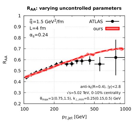
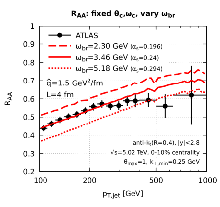
Figure 6: Our MC predictions for $R_{\text{AA}}$ are compared with the results of an experimental analysis by ATLAS Aaboud:2018twu (shown as dots with error bars). Left: the sensitivity of our results to changes in the kinematic cuts $\theta_{\rm max}$ and $k_{\perp,\text{min}}$. Right: the effect of varying $\omega_{\rm br}$ (by $\pm 50\%$) at fixed values for $\omega_{\rm c}$ and $\theta_{c}$.

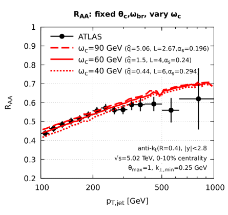
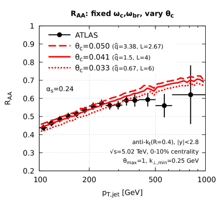
Figure 7: The effects of varying the medium parameters $\hat{q}$, $L$ and ${\alpha}_{s,\text{med}}$ in such a way to keep a constant value for $\omega_{\rm br}$ (the same as the central value in the right plot in Fig. 6, i.e. $\omega_{\rm br}=3.46$ GeV). Left: we vary $\omega_{\rm c}$ by $\pm 50\%$ at fixed $\theta_{c}$. Right: we vary $\theta_{c}^{2}$ by $\pm 50\%$ at fixed $\omega_{\rm c}$.

The first observation, visible in Fig. 6 (left) is that the $R_{AA}$ ratio appears to be very little sensitive to variations of the “unphysical” parameters $\theta_{\rm max}$ and $k_{\perp,\text{min}}$. Although our results for the inclusive jet spectrum do depend on these parameters, the impact on $R_{\text{AA}}$ remains well within the experimental error bars when changing $\theta_{\rm max}$ by a factor 2 and $k_{\perp,\text{min}}$ by a factor larger than 3.

In Fig. 6 right and in the two plots of Fig. 7 we fix the “unphysical” parameters and vary the medium ones. The variations are done, following Table 1, so as to keep two of the three physical scales $\omega_{\rm br}$, $\omega_{\rm c}$ and $\theta_{c}$ fixed while varying the third. It is obvious from the figures that $R_{\text{AA}}$ is most sensitive to variations of $\omega_{\rm br}$ (Fig. 6, right) and shows only a small dependence on $\omega_{\rm c}$ and $\theta_{c}$. This is in perfect agreement with the expectations from section 2.6 that the jet energy loss is mostly driven by the scale $\omega_{\rm br}$. Furthermore, the small variations of $R_{\text{AA}}$ with changes in $\omega_{\rm c}$ and $\theta_{c}$ can be attributed to the slight change in the phase-space for VLEs leading to a corresponding change in the number of sources for energy loss (see section 2.7 and, in particular, Eq. (2.7)).

One remarkable fact about the LHC measurements is the fact that $R_{\text{AA}}$ increases very slowly with the jet $p_{T}$. This implies that the jet energy loss $\mathcal{E}_{\rm{jet}}$ must itself increase with $p_{T}$ to avoid a fast approach of $R_{\text{AA}}$ towards unity. In our picture, such an increase is indeed present, as manifest in Fig. 4, and is associated with the steady rise of the phase-space for VLEs leading to an increase in the number of sources for MIEs (cf. Eq. (2.7)).

5 $z_{g}$ distribution for monochromatic jets

We now turn to a discussion of the $z_{g}$-distribution in the medium. Our purpose is not only to present Monte Carlo simulations, but also to identify the main mechanisms responsible for the various features seen in the simulations. We follow the same strategy as in the previous section, namely we start with “monochromatic” jets initiated by a parton of fixed flavour and $p_{T0}$, a case which is easier to discuss analytically, before we turn (in Sect. 6) to the full $z_{g}$ distribution including the hard process, for which it makes sense to compare our results with the LHC data.

5.1 General definitions and $z_{g}$ in the vacuum

For completeness, we first recall the definition of the soft drop (SD) procedure Larkoski:2014wba . For a given jet of radius $R$, SD first reclusters the constituents of the jet using the Cambridge/Aachen (C/A) algorithm Dokshitzer:1997in ; Wobisch:1998wt . The ensuing jet is then iteratively declustered, i.e. the last step of the pairwise clustering is undone, yielding two subjets of transverse momenta $p_{T1}$ and $p_{T2}$ separated by a distance $\Delta R_{12}=\sqrt{\Delta y_{12}^{2}+\Delta\phi_{12}^{2}}$ in rapidity-azimuth. This procedure stops when the SD condition is met, that is when

$$z_{12}\equiv\frac{\mathrm{min}(p_{T1},p_{T2})}{p_{T1}+p_{T2}}>z_{\text{cut}}\left(\frac{\Delta R_{12}}{R}\right)^{\beta},$$ (22)

where $z_{\text{cut}}$ and $\beta$ are the SD parameters. If the condition is not satisfied, the subjet with the smaller $p_{T}$ is discarded and the declustering procedure continues with the harder. For $\beta=0$, which is what we adopt from now on, the SD procedure coincides with the modified MassDrop Tagger Dasgupta:2013ihk .

With the above procedure, $\theta_{g}$ and $z_{g}$ are defined respectively as $\Delta R_{12}$ and $z_{12}$ for the declustering which satisfied the SD condition. When the declustering procedure reaches a single parton, we set $\theta_{g}$ and $z_{g}$ to zero. Furthermore, one can impose a lower cutoff $\theta_{g}>\theta_{\text{cut}}$. This is commonly used for PbPb collisions at the LHC and is thus our default as well. We then study the differential $z_{g}$ distribution for a jet initiated by a parton of flavour $i$ (quark or gluon). We can consider two possible normalisation for the $z_{g}$ distribution: the “self-normalised” distribution, $p_{i}(z_{g})$, and the “$N_{\text{jets}}$-normalised” distribution, $f_{i}(z_{g})$. The former defined such that

$$\int_{z_{\text{cut}}}^{1/2}{\rm d}z_{g}\,p_{i}(z_{g})=1.$$ (23)

which is equivalent to normalising the $z_{g}$ distribution to the number of jets which pass the SD condition and the optional cut on $\theta_{g}$. The latter is instead normalised to the total number of jets, i.e. the normalisation includes jets which fail either the SD condition or cut on the $\theta_{g}$.

We first recall the basic result for the $z_{g}$-distribution in the vacuum Larkoski:2015lea . The double differential probability for bremsstrahlung starting with a parton of type $i\in\{\text{q,\,g}\}$ reads

$${\rm d}^{2}\mathcal{P}_{i,\text{vac}}(z,\theta)=\frac{2C_{i}\alpha_{s}(zp_{T}\theta_{g})}{\pi}\,\bar{P}_{i}(z)\,{\rm d}z\,\frac{{\rm d}\theta}{\theta}\,\equiv\,\mathcal{P}_{i,\text{vac}}(z,\theta)\,{\rm d}\theta{\rm d}z,$$ (24)

where $\bar{P}_{i}(z)$ is the symmetrised splitting function of a parton of type $i$. The argument of the coupling is the relative transverse momentum of the emission w.r.t. the parent parton. We can also introduce the “Sudakov factor” $\Delta_{i}(R,\theta_{g})$, which is the probability to have no emission at any angle between $\theta_{g}$ and $R$ and with any splitting fraction $z\geq z_{\text{cut}}$:

$$\Delta_{i}(R,\theta_{g})=\exp\left(-\int_{\theta_{g}}^{R}{{\rm d}\theta}\int_{z_{\text{cut}}}^{1/2}{\rm d}z\,\,\mathcal{P}_{i,\,\text{vac}}(z,\theta)\right)\,.$$ (25)

The $z_{g}$-distribution is obtained by considering the probability for both $z_{g}$ and $\theta_{g}$, marginalised over $\theta_{g}$. The former is simply expressed as the probability to have no branching between $\theta_{g}$ and $R$ times the probability of a branching with $\theta=\theta_{g}$ and $z=z_{g}$, so that

$$p_{i,\text{vac}}(z_{g})=\frac{\Theta(z_{g}-z_{\text{cut}})}{1-\Delta_{i}(R,\theta_{\text{cut}})}\int_{\theta_{\text{cut}}}^{R}{\rm d}\theta_{g}\,\mathcal{P}_{i,\text{vac}}(z_{g},\theta_{g})\Delta_{i}(R,\theta_{g}),$$ (26)

where we have included an optional cut $\theta_{g}>\theta_{\text{cut}}$. The overall factor $(1-\Delta_{i})^{-1}$ enforces the normalisation condition (23). It would be equal to one in the absence of the minimal angle $\theta_{\text{cut}}$. This also means that $f_{i}(z_{g})$ coincides with $p_{i}(z_{g})$ in the limit $\theta_{\text{cut}}\to 0$.

In this context, it is worth pointing out that, in the limit $\theta_{\text{cut}}\to 0$, $z_{g}$ is a peculiar observable from the point of view of perturbative QCD. Indeed, while Eq. (26) is overall finite, its expansion at any finite order of perturbation theory is collinearly divergent, due to the fact that $\mathcal{P}_{i,\text{vac}}(z_{g},\theta_{g})$ diverges when $\theta_{g}\to 0$. It is only after an all-order resummation that the exponential form of the Sudakov regulates the divergence. In other words, although $z_{g}$ is collinear unsafe, it is Sudakov safe Larkoski:2015lea .

To discuss the physics underlying the $z_{g}$ distribution, it is sometimes helpful to consider the fixed-coupling approximation. One can then easily perform the angular integration in Eq. (26) and get

$$p_{i,{\text{vac}}}(z_{g})=\frac{\bar{P}_{i}(z_{g})}{\int_{z_{\text{cut}}}^{1/2}\bar{P}_{i}(z)dz}\Theta(z_{g}-z_{\text{cut}}).$$ (27)

This makes it clear that the $z_{g}$-distribution provides a direct measurement of the splitting function.

5.2 In-medium $z_{g}$ distribution: Monte Carlo results

We now present our Monte Carlo results for the $z_{g}$-distribution created by “monochromatic” jets which propagates through the quark-gluon plasma. We focus on the $N_{\text{jets}}$-normalised distribution $f_{i,\text{med}}(z_{g})$, which carries more information. We define the corresponding nuclear modification factor, $\mathcal{R}_{i}(z_{g})\equiv f_{i,\text{med}}(z_{g})/f_{i,\text{vac}}(z_{g})$. Similarly we define $\mathcal{R}_{i}^{\text{(norm)}}(z_{g})\equiv p_{i,\text{med}}(z_{g})/p_{i,\text{vac}}(z_{g})$ as the nuclear modification factor of the self-normalised $z_{g}$ distributions. We study four different values for the initial $p_{T0}$ spanning a wide range in $p_{T0}$, from $100$ GeV to $1$ TeV. We use the same SD parameters as in the CMS analysis Sirunyan:2017bsd , namely $\beta=0$ and $z_{\text{cut}}=0.1$, together with a cut $\theta_{g}>\theta_{\text{cut}}=0.1$. In this section we mostly highlight the main features of our Monte Carlo simulations and provide a brief physical interpretation. More detailed analytic calculations are postponed to sections 5.3 for high-energy jets and 5.4 for lower-energy jets.

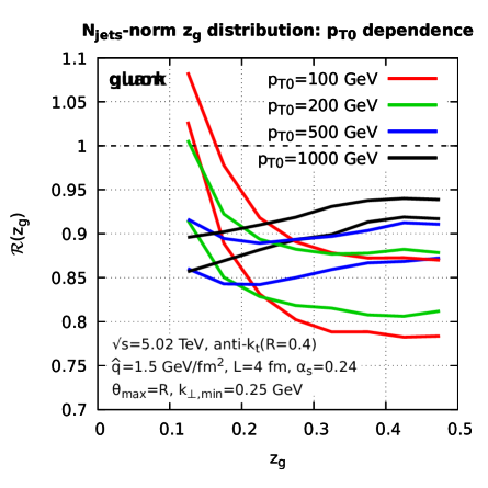
Figure 8: A summary of our MC results for the medium/vacuum ratio $\mathcal{R}_{i}(z_{g})$ of the $N_{\text{jets}}$-normalised distributions, for monochromatic jets initiated either by a gluon (left figure), or by a quark (right figure), and for 4 different values for the initial transverse momentum $p_{T0}$.

Our results are shown in Fig. 8, separately for jets initiated by a gluon (left plot) and by a quark (right plot), using our default MC parameters (cf. Table 1). As for our study of energy loss for monochromatic jets in section 4, we set the angular cutoff scale of our Monte Carlo to $\theta_{\text{max}}=R$ with $R=0.4$ the jet radius. Each of the plots in Fig. 8 show qualitatively different behaviours between our lowest $p_{T0}$ (100 GeV) value and the largest one (1 TeV). More precisely, for the highest energy jets, $p_{T0}=1$ TeV, the ratio $\mathcal{R}(z_{g})$ is always smaller than one, indicating a nuclear suppression, and it increases monotonously with $z_{g}$, meaning that the nuclear suppression is larger at small $z_{g}$. Conversely, for lower $p_{T0}$, while the nuclear suppression becomes stronger at large $z_{g}$, a peak develops at small $z_{g}$ where $\mathcal{R}(z_{g})$ can even become larger than one, indicating a nuclear enhancement.

Let us first discuss the behaviour at large $p_{T0}$, focusing on $p_{T0}=1$ TeV. In this case, the softest radiation that can be captured by Soft Drop has an energy $z_{\text{cut}}p_{T0}=100$ GeV which is still larger than the hardest medium-induced emissions which have energies $\omega\sim\omega_{\rm c}=60$ GeV. Hence, for jets with high-enough $p_{T0}$, SD can only select vacuum-like emissions. To illustrate this, we show in the left plot of Fig. 9 the phase-space selected by SD. Under these circumstances, the only nuclear effect on the $z_{g}$-distribution is the energy lost by the two (hard, $z_{g}>z_{\text{cut}}$) subjets passing the SD condition. Due to this energy loss, the effective splitting fraction $z_{g}$ measured by SD turns out to be slightly smaller than the physical splitting fraction $z$ at the branching vertex (see Sect. 5.3 for details). If we call for now this shift $\Delta z=z-z_{g}>0$, we have (cf. (27))

$$\mathcal{R}(z_{g})\approx\frac{\bar{P}_{g}(z=z_{g}+\Delta z)}{\bar{P}_{g}(z_{g})}\,\simeq\,\frac{z_{g}}{z_{g}+\Delta z}\,\simeq\,1-\frac{\Delta z}{z_{g}}\quad\mbox{for \ $\Delta z\ll z_{g}\ll 1$}\,,$$ (28)

which explains the pattern (smaller than one and increasing with $z_{g}$) observed at large $p_{T0}$ in Fig. 8.

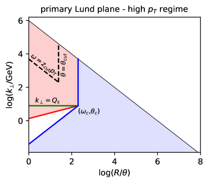
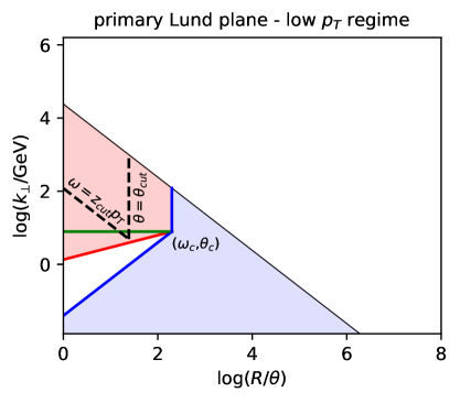
Figure 9: The kinematic regions in the Lund plane that are covered by the SD algorithm in the case of a high-energy jet ($z_{\text{cut}}p_{T}>\omega_{\rm c}$) in the left figure and of a low-energy jet ($z_{\text{cut}}p_{T}<\omega_{\rm c}$) in the right figure. As suggested by the pictorial representation in the right figure, the most interesting situation for “low-energy jets” is such that there is only little overlap between the kinematic region for SD and the phase-space for MIEs.

The above discussion also suggests what changes when moving to the opposite regime of (relatively) low energy jets, say $p_{T0}=100$ GeV. In this case, the energy interval covered by SD, that is $\omega$ between $z_{\text{cut}}p_{T0}=10\,{\rm GeV}$ and $p_{T0}/2=50$ GeV, fully overlaps with the BDMPS-Z spectrum for medium-induced radiation which has $\omega\lesssim\omega_{\rm c}=60$ GeV (cf. the right plot of Fig. 9). Consequently, the SD condition can now be triggered either by a vacuum-like splitting, or by a medium-induced one. Since the BDMPS-Z spectrum increases rapidly at small $z$ (faster than the vacuum splitting function), this naturally explains the peak in the ratio $\mathcal{R}(z_{g})$ at small $z_{g}$, visible in Fig. 8. The nuclear suppression observe at large $z_{g}$ suggests that in this region, the energy loss effects dominate over the BDMPS-Z emissions.

The above arguments show that the $z_{g}$ distribution is best discussed separately for high-energy and low-energy jets, where the separation between the two regimes is set by the ratio $z_{\text{cut}}p_{T0}/\omega_{\rm c}$. The high-energy jets, for which $p_{T0}>\omega_{\rm c}/z_{\text{cut}}$, are conceptually simper as the in-medium $z_{g}$ distribution is only affected by the energy loss via MIEs. For low-energy jets, i.e. jets with $p_{T0}<\omega_{\rm c}/z_{\text{cut}}$, the $z_{g}$ distribution is affected by the medium both directly when the SD condition is triggered by a MIE, and indirectly via the energy loss of the two subjets emerging from the hard splitting. This second case is more complex for a series of reasons and notably because MIEs do not obey angular ordering.

Since $z_{g}$ is intrinsically tied to energy loss effects, it is interesting to study how the average jet energy loss correlates with $z_{g}$. Our numerical results are presented in Fig. 10. The dashed curve shows the MC results for the inclusive jets (all values of $z_{g}$), the one denoted “no $z_{g}$” refers to jets which did not pass the SD criterion or failed the cut $\theta_{g}>\theta_{\text{cut}}$, and the other curves correspond to different bins of $z_{g}$. One clearly sees a distinction between the “no $z_{g}$” jets, which lose much less energy than the average jet, and those which passed SD, whose energy loss is larger than the average and quasi-independent of $z_{g}$. The main reason for this behaviour is that jets passing the SD condition are effectively built of two relatively hard subjets. Since the angular separation between these two hard subjets is larger than $\theta_{\text{cut}}=0.1>\theta_{c}\simeq 0.04$, they lose energy (via MIEs) as two independent jets, giving a larger-than-average energy loss. This is mostly controlled by the geometry of the system, with only a limited sensitivity to the precise sharing of the energy between the subjets. On the other hand, the jets which did not pass SD are typically narrow one-prong jets with either no hard substructure or with some substructure at an angle smaller that $\theta_{\text{cut}}=0.1$ (i.e. at an angle $\simeq\theta_{c}$). These jet therefore lose less energy that an average jet. The fact that the angular cutoff $\theta_{\text{cut}}=0.1$ is close to the critical value $\theta_{c}\simeq 0.04$ is clearly essential for the above arguments.

A last comment concerns the difference between the $z_{g}$-distributions for gluon- and quark-initiated jets, as shown in the left and right plots of Fig. 8, respectively. The deviation of the medium/vacuum ratio from unity appears to be larger for quark jets than for gluon jets. This might look surprising at first sight given that the average energy loss is known to be larger for the gluon jet than for the quark one (cf. Figs. 4 and 5). However we will show in section 5.3 that the $z_{g}$ distribution is mostly controlled by the energy loss of the softest subjet, which is typically a gluon jet even when the leading parton is a quark. The difference between quark and gluon jets in Fig. 8 is in fact controlled by “non-medium” effects, like the difference in their respective splitting functions.

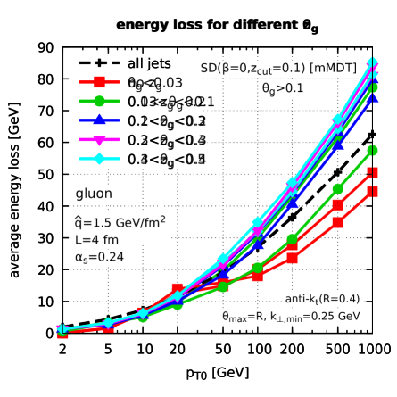
Figure 10: Our MC results for the average energy loss by a gluon-initiated jet are displayed as a function of the initial gluon energy $p_{T0}$ in bins of $z_{g}$. The inclusive (all jets) result is also shown, by the dashed line.

5.3 Analytic insight for high-energy jets: VLEs and energy loss

We begin our analytic calculations of the nuclear effects on the $z_{g}$ distribution with the case of a high-energy jet, $p_{T0}>\omega_{\rm c}/z_{\text{cut}}$ In this case, the SD condition is triggered by an in-medium VLE that we call the “hard splitting” in what follows. This splitting occurs early (since $t_{\rm f}\ll L$, cf. Eq. (3)) and the daughter partons propagate through the medium over a distance of order $L$. During their propagation, they evolve into two subjets, both via VLEs (which obey angular ordering, except possibly for the first emission outside the medium) and via MIEs (which can be emitted at any angle).

Since the C/A algorithm is used by the SD procedure, both subjets have an opening angle of order $\theta_{g}$, with $\theta_{g}$ the angle of the hard splitting. Consequently, the emissions from the two subjets with angles larger than $\theta_{g}$ — either MIEs, or VLEs produced outside the medium — are not clustered within the two subjets. Accordingly, their reconstructed transverse momenta $p_{T1}$ and $p_{T2}$ are generally lower than the initial momenta, $\omega_{1}$ and $\omega_{2}$, of the daughter partons produced by the hard splitting. This implies a difference between the reconstructed splitting fraction $z_{g}=p_{T,1}/(p_{T,1}+p_{T,2})$ and the physical one, $z\equiv\omega_{1}/(\omega_{1}+\omega_{2})$. This difference is controlled by the energy lost by the two subjets.

Let us first mention that the energy loss via VLEs outside the medium at angles $\theta>\theta_{g}$ can be neglected. Indeed, since these emissions have $t_{\rm f}\sim 1/(\omega\theta^{2})>L$, they are soft and only give very small contributions to the energy loss. We have checked this explicitly with MC studies of the VLEs alone: we find that the effect on the $z_{g}$ distribution of the vetoed region and of the violation of angular ordering for the first emission outside the medium are much smaller than those associated with the energy loss via MIEs.

We then discuss the role of colour coherence for the energy loss via MIEs. If the splitting angle $\theta_{g}$ is smaller than $\theta_{c}$ the daughter partons are not discriminated by the medium. This is a case of coherent energy loss where the MIEs at angles $\theta>\theta_{g}$ are effectively sourced by their parent parton MehtarTani:2010ma ; MehtarTani:2011tz ; CasalderreySolana:2011rz ; CasalderreySolana:2012ef , so that $z=z_{g}$. On the other hand, for larger splitting angles $\theta_{g}\gg\theta_{c}$, the colour coherence is rapidly washed out, so the two daughter partons act as independent sources of MIEs. In this case, one can write $\omega_{i}=p_{Ti}+\mathcal{E}_{i}(\omega_{i},\theta_{g})$, where $i=1,2$ and $\mathcal{E}_{i}(\omega_{i},\theta_{g})$ is the average energy loss for a jet of flavour $i$, initial energy $\omega_{i}$ and opening angle $\theta_{g}$ (cf. e.g. Eq. (2.7)). It would be relatively straightforward to deal with generic values of $\theta_{g}$, both coherent and incoherent. In practice, all existing measurements at the LHC imposes a minimal angle $\theta_{g}\geq\theta_{\text{cut}}$, with $\theta_{\text{cut}}=0.1$. Since $\theta_{\text{cut}}$ is larger than $\theta_{c}$ for all our choices of parameters, we only consider the incoherent case $\theta_{g}>\theta_{\text{cut}}$ in what follows.

That said, the relation between the measured $z_{g}$ and the physical splitting fraction $z$ can be written as (assuming $p_{T1}<p_{T2}$)

$$z_{g}=\frac{p_{T1}}{p_{T1}+p_{T2}}=\frac{zp_{T}-\mathcal{E}_{1}(zp_{T},\theta_{g})}{p_{T}-\mathcal{E}_{1}(zp_{T},\theta_{g})-\mathcal{E}_{2}((1-z)p_{T},\theta_{g})}\,\equiv\,\mathcal{Z}_{g}(z,\theta_{g})\,,$$ (29)

where $p_{T}\equiv\omega_{1}+\omega_{2}$ is the energy (or transverse momentum) of the parent parton at the time of the “hard” branching. In what follows we approximate $p_{T}\simeq p_{T,0}$. This is valid as long as one can neglect two effects: (i) the transverse momentum of the partons which have been groomed away during previous iterations of the SD procedure, and (ii) MIEs prior to the hard branching. The former is indeed negligible as long as we work in the standard limit $z_{\text{cut}}\ll 1$, and the latter is also negligible based on our short formation time arguments in section 2.2.

For a given average energy loss $\mathcal{E}(p_{T},\theta_{g})$ one can, at least numerically, invert Eq. (29) to obtain the physical splitting fraction $z=\mathcal{Z}(z_{g},\theta_{g})$ corresponding to the measured $z_{g}$. The kinematic constraint $z_{g}>z_{\text{cut}}$ thus implies a constraint on $z$, $z\geq\mathcal{Z}(z_{\text{cut}},\theta_{g})$, and the in-medium $z_{g}$ distribution in this high-energy regime becomes a straightforward generalisation of Eq. (26)

$$p_{i,\text{med}}(z_{g})=\mathcal{N}\int_{\theta_{\text{cut}}}^{R}{\rm d}\theta_{g}\,\Delta_{i}^{\text{VLE}}(R,\theta_{g})\int_{0}^{1/2}{\rm d}z\,\mathcal{P}_{i,\text{vac}}(z,\theta_{g})\,\delta\big{(}z_{g}\!-\!\mathcal{Z}_{g}(z,\theta_{g})\big{)}\Theta(z_{g}\!-\!z_{\text{cut}}),$$ (30)

where the Sudakov factor is formally the same as in the vacuum, Eq. (25), but with the new, medium-dependent, lower limit $\mathcal{Z}(z_{\text{cut}},\theta)$ on $z$:

$$\Delta_{i}^{\text{VLE}}(R,\theta_{g})=\exp\left(-\int_{\theta_{g}}^{R}{{\rm d}\theta}\int_{0}^{1/2}{\rm d}z\,\,\mathcal{P}_{i,\text{vac}}(z,\theta)\,\Theta\big{(}z-\mathcal{Z}(z_{\text{cut}},\theta)\big{)}\right)\,.$$ (31)

The normalisation factor $\mathcal{N}$ in (30) is given by $(1-\Delta_{i}^{\text{VLE}})^{-1}$. The $N_{\text{jets}}$-normalised distribution $f_{i,\text{med}}(z_{g})$ is obtained by simply removing this factor $\mathcal{N}$.

In practice we will replace $\theta_{g}$ by $R$ in the argument of the energy loss. This is motivated by two facts. Firstly, due to the SD procedure, we know that the jet is free of emissions with $\omega>z_{\text{cut}}p_{T0}$ at angles between $\theta_{g}$ and $R$, simply because such an emission would have triggered the SD condition. The remaining emissions between $\theta_{g}$ and $R$ are therefore soft and we neglect them. Secondly, the angular phase-space $\theta_{\text{cut}}<\theta<R$ is relatively small and $\mathcal{E}$ is slowly varying over this domain. With this approximation, both $\mathcal{Z}_{g}$ and $\mathcal{Z}$ becomes independent of $\theta_{g}$ and the Sudakov factor (31) simplifies to the vacuum one, Eq. (25), evaluated at $z_{\text{cut}}\to\mathcal{Z}(z_{\text{cut}})$.

The above picture can be further simplified by noticing that the energy losses are typically much smaller than $zp_{T}$ and $(1-z)p_{T}$. This means that the difference between $z$ and $z_{g}$ is parametrically small and we can replace $z$ by $z_{g}$ in the arguments of the energy loss in (29) so that

$$z\equiv\mathcal{Z}(z_{g},\theta_{g})\simeq\,z_{g}+\,\frac{\mathcal{E}_{1}-z_{g}(\mathcal{E}_{1}+\mathcal{E}_{2})}{p_{T}}\,,$$ (32)

with $\mathcal{E}_{1}\equiv\mathcal{E}_{1}(z_{g}p_{T})$ and $\mathcal{E}_{2}\equiv\mathcal{E}_{2}((1-z_{g})p_{T})$. Since $z_{g}<1/2$, this shows that the physical $z$ is typically larger than $z_{g}$.

As before, it is useful to consider the fixed-coupling scenario where the $z_{g}$-dependence of Eq. (30) factorises from the integral over $\theta_{g}$. After dividing out by the vacuum distribution $\propto\bar{P}_{i}(z_{g})$, we find

$$\mathcal{R}(z_{g})\equiv\frac{f_{\text{med}}(z_{g})}{f_{\text{vac}}(z_{g})}\simeq\mathcal{J}(z_{g})\,\frac{\bar{P}_{g}(\mathcal{Z}(z_{g}))}{\bar{P}_{g}(z_{g})}\,,\qquad\mbox{with}\quad\mathcal{J}(z_{g})\equiv\bigg{|}\frac{{\rm d}\mathcal{Z}(z_{g})}{{\rm d}z_{g}}\bigg{|}\simeq 1-\frac{\mathcal{E}_{1}+\mathcal{E}_{2}}{p_{T}}\,,$$ (33)

where $\mathcal{J}$ is a Jacobian and the last equality in (33) is obtained using the simplified expression (32).

At this level, it becomes necessary to specify the energy lost by a subjet. At high energy, both $zp_{T}$ and $(1-z)p_{T}$ are large and the energy lost by the subjets is sensitive to the increase in the number of partonic sources for MIEs (cf. section 2.7 and Fig. 4). To test this picture, we consider two energy loss scenarios. First, the case of an energy loss which captures the increase in the number of sources for MIEs and increases with the jet $p_{T}$, as in Eq. (2.7). Since Eq. (2.7) is not very accurate we will instead use $\mathcal{E}_{j}=\mathcal{E}_{j,\text{fit}}$ corresponding to the fit of the Monte Carlo result shown in Fig. 4. The second scenario corresponds to what would happen in the absence of VLEs, i.e. when only MIEs from the leading parton in each subjet are included. This gives an energy loss which saturates to a constant $\mathcal{E}_{j}=\varepsilon_{j}$ at large $p_{T}$ (see again Fig. 4). Clearly, the first scenario is the most physically realistic.

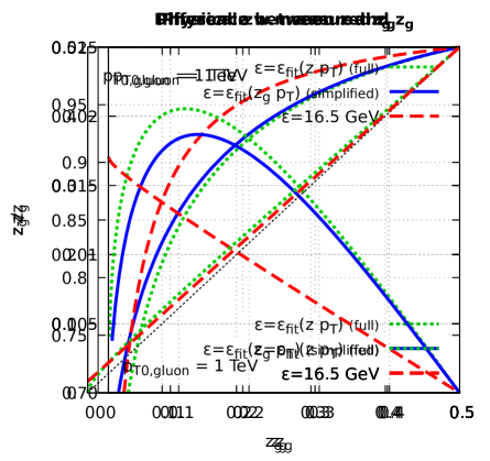
Figure 11: The ratio $z_{g}/z$ (left figure) and the difference $z-z_{g}$ (right figure) between the splitting fraction $z_{g}$ measured by SD and the physical splitting fraction $z$ for the hard splitting. This difference is given by Eq. (29) that we evaluate with two scenarios for the energy loss by the subjets: a constant energy loss and a $p_{T}$-dependent one; for the second scenario, we also show the predictions of the simplified relation (32).

For definiteness, let us first consider the case of a 1-TeV gluon-initiated jet. Fig. 11 shows the relation between the physical splitting fraction $z$ and the measured $z_{g}$, with the ratio $z_{g}/z$ plotted on the left panel and the difference $z-z_{g}$ on the right panel. We see that $z$ is larger than $z_{g}$ in both energy-loss scenarios. The difference $z-z_{g}$ decreases when increasing $z$ (at least for $z>z_{\text{cut}}$), while the ratio $z_{g}/z$ gets close to 1. The effects are roughly twice as large for the full energy-loss scenario than for a constant energy loss. The dotted (green) curve shows the result obtained using the “full” relation (29) while the solid (blue) line uses the simplified version, Eq (32). As expected, they both lead to very similar results and we therefore make the simplified version our default from now on.

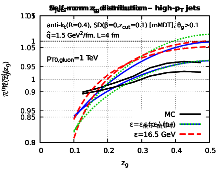
Figure 12: Our MC results for the medium/vacuum ratio of the $z_{g}$ distributions associated with gluon-initiated jets with initial energy $p_{T0}=1$ GeV are compared to our analytic predictions for the two scenarios of energy loss described in the text. The left plot refers to the self-normalised distributions, cf. Eq. (30), and the right plot to the $N_{\text{jets}}$-normalised ones.

The nuclear modification factor for the $z_{g}$ distribution obtained from our analytic calculation (30), including running-coupling corrections, is shown in Fig. 12 for both the self-normalised distribution $p_{\text{med}}(z_{g})$ (left) and the $N_{\text{jets}}$-normalised one $f_{\text{med}}(z_{g})$ (right). We see that $\mathcal{R}(z_{g})$ increases with $z_{g}$. This is expected since, at small $z_{g}$, $\bar{P}_{g}(z)/\bar{P}_{g}(z_{g})\simeq z_{g}/z$ which increases with $z_{g}$ (see e.g. Fig. 11, left). Furthermore, the medium/vacuum ratio of the $N_{\text{jets}}$-normalised distributions (Fig. 12, right) is always smaller than one. With reference to the fixed-coupling estimate in Eq. (33), this is a combined effect of $z$ being larger than $z_{g}$, hence $\bar{P}_{g}(z)<\bar{P}_{g}(z_{g})$, and of the extra Jacobian in front of Eq. (33).

Regarding the comparison between the two scenarios for the energy loss, we see that although they produce similar results for the self-normalised $z_{g}$ distribution, the (physical) “full jet” scenario predicts a larger suppression than the “constant” one for the medium/vacuum ratio of the $N_{\text{jets}}$-normalised distributions. In particular, the former predicts a value for $\mathcal{R}(z_{g})$ which remains significantly smaller than one even at $z_{g}$ close to 1/2. This behaviour is in also in better agreement with our Monte Carlo simulations. Generally speaking, it is worth keeping in mind that the $N_{\text{jets}}$-normalised ratio is better suited to disentangle between different energy-loss models than the self-normalised ratio which is bound to cross one by construction.

Since the nuclear modification of the $z_{g}$ distribution appears to be so sensitive to the energy loss, it is interesting to check whether this observable follows the Casimir scaling of the jet energy loss. We show that this is not the case and that the nuclear modification is even slightly larger for quark than for gluon jets. In practice, the $z_{g}$ distribution is controlled by the energy loss of the softest among the two subjets created by the hard splitting, which is typically a gluon independently of the flavour of the initial parton. Let us then consider Eq. (32) in which we take $\mathcal{E}_{1}=\mathcal{E}_{\text{g}}$ and $\mathcal{E}_{2}=\mathcal{E}_{R}$, with $R={\text{q}}$ or g depending on the colour representation of the leading parton. Simple algebra yields

$$z^{(\text{g-jet})}(z_{g})\,\simeq\,z^{(\text{q-jet})}(z_{g})+z_{g}\,\frac{\mathcal{E}_{\text{g}}-\mathcal{E}_{\text{q}}}{p_{T}}$$ (34)

where $z^{(R\text{-jet})}(z_{g})$ is the physical splitting fraction $z$ corresponding to a measured fraction $z_{g}$ for the case of a leading parton of flavour $R$, and the energy loss functions $\mathcal{E}_{R}$ are evaluated at $(1-z_{g})p_{T}$. Since $\mathcal{E}_{\text{g}}\simeq 2\mathcal{E}_{\text{q}}$ the second term in (34) is positive and thus $z^{(\text{g-jet})}(z_{g})>z^{(\text{q-jet})}(z_{g})$ as expected on physical grounds. Yet, the difference between $z^{(\text{g-jet})}(z_{g})$ and $z^{(\text{q-jet})}(z_{g})$ is weighted by $z_{g}$, hence it suppressed at small $z_{g}$, where the energy loss effects should be more important. Furthermore, the effects of the difference $z^{(\text{g-jet})}(z_{g})-z^{(\text{q-jet})}(z_{g})$ are difficult to distinguish in practice since there are other sources of differences between the $z_{g}$ distributions of quark and gluon jets like the non-singular terms in the splitting functions and the different Sudakov factors. In practice these effects appear to dominate over difference between $z^{(\text{g-jet})}(z_{g})$ and $z^{(\text{q-jet})}(z_{g})$

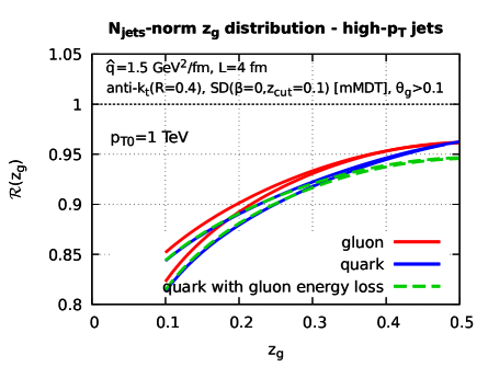
Figure 13: The results of the analytic calculations for the medium/vacuum ratio $\mathcal{R}(z_{g})$ for both gluon- and quark-initiated jets, together with the fictitious case where a quark-initiated subjet loses the same amount of energy as a gluon-initiated one.

This is confirmed by our analytic calculations in Fig. 13. Together with our previous results for a gluon jet, we show two scenarios for quark jets: (a) a realistic scenario which takes into account the different quark and gluon energy losses (cf. Fig. 4), and (b) a fictitious case, which assumes that a quark subjet loses the same energy as a gluon one, i.e. $\mathcal{E}_{\text{q}}=\mathcal{E}_{\text{g}}$. In both cases, the nuclear suppression of the $z_{g}$ distribution appears larger for quark-initiated jets than for gluon-initiated jets, in qualitative agreement with our Monte Carlo findings (recall Fig. 8). This is clearly driven by effects beyond the energy loss difference between quarks and gluons (cf our case (b)), even though this difference has indeed the effect of slightly increasing $\mathcal{R}(z_{g})$, especially close to $z_{g}=1/2$, as visible by comparing the curves corresponding to the cases (a) and (b).

In summary, the main lessons one draws from our study of high-energy jets are as follows: (i) the incoherent energy loss by the two subjets created by the hard splitting leads to a suppression in the nuclear $z_{g}$ distribution which is larger at small $z_{g}$; (ii) the MC results are sensitive to the evolution of the subjets multiplicity via VLEs which leads to an energy loss increasing with the subjet $p_{T}$; (iii) this last effect may be hidden when studying the self-normalised $z_{g}$ distribution; in that respect, the $N_{\text{jets}}$-normalised distribution is better suited to disentangle between different energy-loss models.

5.4 Analytic insight for low-energy jets: MIEs and energy loss

We now turn to more phenomenologically-relevant case of “low energy” jets, $p_{T0}<\omega_{c}/z_{\text{cut}}$ (with $\omega_{c}/z_{\text{cut}}=600$ GeV for our default choice of medium parameters), for which the “hard” emission that triggers the SD condition can be either vacuum-like or medium-induced. In both cases, the two ensuing subjets lose energy via MIEs, which, as explained in the previous section, implies that the measured value $z_{g}$ is different (typically slightly smaller) than the physical value $z$.

Our main goal in this section is to develop analytic approximations which qualitatively and even semi-quantitatively capture this complex dynamics. For definiteness, we focus on gluon-initiated jets with $p_{T0}=200$ GeV. This value is at the same time low enough to be representative for the low-energy regime and large enough to justify some convenient approximations, like the single emission approximation for the MIEs captured by SD. For pedagogical reasons it is convenient to first consider two simplified situations — a jet built with MIEs alone and a jet in which the SD condition can only be triggered by a VLE (as in the “high-energy” case) —, before addressing the full picture in Sect. 5.4.3.

5.4.1 Low-energy jets: medium-induced emissions only

To study the case where the SD condition is triggered by a MIE, we consider jets generated via MIEs only, disabling VLEs. Since the emission angles of MIEs are controlled by their transverse momentum broadening (cf. Sect. 2.5), they are not ordered in angle. Hence, the reclustering of the jet constituents with the C/A algorithm does not necessarily respects the physical ordering of the MIEs in time. In particular, the branching selected by the SD procedure may not be a primary emission, i.e. a direct emission by the leading parton. However, as long as $z_{\text{cut}}p_{T0}$ is sufficiently large compared to the characteristic scale $\omega_{\rm br}=3.46$ GeV for multiple branching — which is definitely the case for our 200 GeV jets, — the probability to select a non-primary branching is suppressed by ${\alpha}_{s,\text{med}}$. From now on we can therefore assume that SD selects a primary MIE.

Next, we can argue that the MIEs captured by the SD algorithm are soft and located in a small corner near $z=z_{\text{cut}}$ and $\theta=\theta_{\text{cut}}$. Indeed, the bulk of the MIEs lies below the line $k_{\perp}=Q_{s}=2.4$ GeV and the smallest value of $k_{\perp}$ that can be selected by SD, namely $z_{\text{cut}}p_{T0}\theta_{\text{cut}}=2$ GeV, is only slightly smaller than $Q_{s}$. This is visible in the phase-space diagram of Fig. 9 (right). Together with the fact that the BDMPS-Z rate (7) grows quickly as $z\to 0$, this means that MIEs contribute to the $z_{g}$ distribution only at small $z_{g}$. After SD, one therefore has a soft subjet of transverse momentum $p_{T1}$ corresponding to the MIE and a harder subjet of momentum $p_{T2}$ corresponding to the leading parton.

The differential probability for the emission of a primary MIE with $\omega_{1}\equiv\omega\ll p_{T0}$ is given by the BDMPS-Z spectrum (8) multiplied by the angular distribution produced via transverse momentum broadening after emission, Eq. (11). The latter depends on the distance $\Delta t=L-t$, with $t$ the emission time, travelled by the two subjets through the medium. In principle one should therefore work differentially in $t$. Since this would be a serious complication, we rather use a picture in which we average over all the emission times $t$, distributed with uniform probability over the interval $0<t<L$. The differential probability for the “hard” splitting then takes the form

$${\rm d}^{2}\mathcal{P}_{i,\text{med}}(\omega,\theta)=\frac{C_{i}{\alpha}_{s,\text{med}}}{\pi}\Theta\left({\omega_{\rm c}}-\omega\right)\sqrt{\frac{2\omega_{\rm c}}{\omega^{3/2}}}\,\mathcal{P}_{\text{broad}}(\omega,\theta)\,{{\rm d}\omega}{\rm d}\theta\,\equiv\,\mathcal{P}_{i,\text{med}}(\omega,\theta){\rm d}\omega{\rm d}\theta,$$ (35)

where Mehtar-Tani:2016aco

$$\mathcal{P}_{\text{broad}}(\omega,\theta)\equiv\frac{1}{L}\int_{0}^{L}{\rm d}t\,\frac{2\omega^{2}\theta}{\hat{q}(L-t)}\exp\left\{-\frac{\omega^{2}\theta^{2}}{\hat{q}(L-t)}\right\}=2\theta\,\frac{\omega^{2}}{Q_{s}^{2}}\,\Gamma\left(0,\frac{\omega^{2}\theta^{2}}{Q_{s}^{2}}\right),$$ (36)

with $\Gamma(0,x)$ the incomplete Gamma function. This distribution predicts an average value $\bar{k}_{\perp}=\tfrac{\sqrt{\pi}}{3}Q_{s}$ for $k_{\perp}\equiv\omega\theta$. It shows a peak near $\bar{k}_{\perp}$, and a rather wide tail at larger values $k_{\perp}>\bar{k}_{\perp}$ (see Fig. 14, left). Since we have just argued that SD selects emissions in a narrow range in $k_{\perp}$, close to $Q_{s}$, the tail of this distribution plays an important role in our discussion. This is amplified by the fact that $\bar{k}_{\perp}$ is slightly smaller than $Q_{s}$. Note that in terms of the emission angle, this argument means that the emissions selected by SD will need to acquire a $\theta$ larger than the peak value $\bar{\theta}(\omega)=\bar{k}_{\perp}/\omega$ from broadening in order to pass the $\theta_{\text{cut}}$ condition. In future work, it will be interesting to study how a description of broadening beyond the Gaussian approximation affects quantitatively our results.

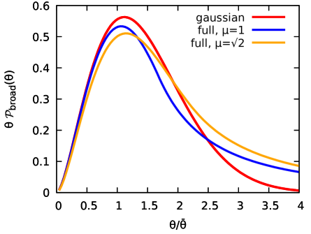
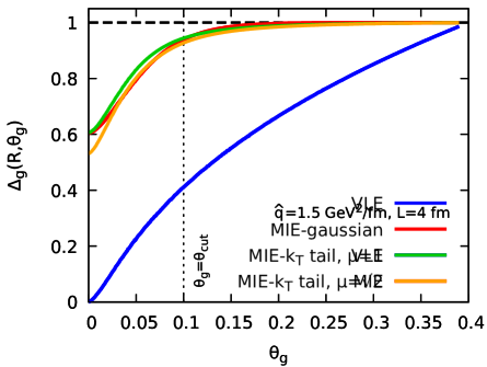
Figure 14: Left: after multiplication by $\theta$, the angular distribution $\mathcal{P}_{\text{broad}}$ in Eq. (36) scales as a function of the ratio $\theta/\bar{\theta}$, with $\bar{\theta}=(\sqrt{\pi}/3)Q_{s}/\omega$. Right: the Sudakov factors $\Delta_{\text{g}}^{\text{MIE}}(R,\theta_{g})$ for MIEs, cf. Eq. (39), and $\Delta_{\text{g}}^{\text{VLE}}(R,\theta_{g})$ for VLEs, cf. Eq. (31), for a gluon-initiated jet with $p_{T0}=200$ GeV and $R=0.4$.

Additionally, we need to account for the fact that both the MIE that triggers the SD condition and the leading parton lose energy. The situation is mostly the same as for our earlier high-energy case except that now the medium-induced gluon emission can occur anywhere inside the medium, i.e. at any time $t$ with $0<t<L$. For an emitted gluon of energy $\omega$, one can write $p_{T1}=\omega-\varepsilon_{\text{g}}(\omega,\theta_{g},\Delta t)$, where the energy loss depends explicitly on the distance $\Delta t=L-t$ travelled by the subjet through the medium. In our kinematic range, this energy loss is relatively small, $\varepsilon_{\rm g}\ll\omega$, and therefore varies slowly with $\omega$ (cf. Eq. (15) so we can neglect the $\omega$ dependence. It depends however quadratically on $\Delta t$. For simplicity, we use a time-averaged picture in which $\langle t\rangle\simeq\langle\Delta t\rangle\simeq L/2$ and therefore $\varepsilon_{\text{g}}(\Delta t)\approx\varepsilon_{\text{g}}(L/2)\simeq\tfrac{1}{4}\varepsilon_{\text{g}}(L)\equiv\bar{\varepsilon}_{\text{g}}$, with $\varepsilon_{\text{g}}(L)\propto L^{2}$ the energy loss corresponding to a distance $L$.

The situation for the harder subjet matching with the leading parton, is more complex, owing to differences between the time ordering of MIEs and the (angular-ordered) C/A clustering used by SD. Indeed, MIEs from the leading parton at times smaller than $t$ and angles smaller than $\theta_{g}$ will be clustered by the C/A algorithm in the harder subjet. These emissions can carry a substantial amount of energy so that, without a full picture of the time evolution of the jet, it is delicate to even define a physical transverse momentum, $\omega_{2}$, for the harder subjet at the vertex where the MIE triggering the SD condition is emitted. We can however take a different approach and realise that, by definition, the difference $p_{T0}-(p_{T1}+p_{T2})$ corresponds to the energy $\varepsilon_{i}(p_{T0},\theta_{g})$ lost by the initial parton at angles larger than $\theta_{g}$. As for the high-energy case, we can neglect the energy lost between $\theta_{g}$ and $R$ and hence write $p_{T1}+p_{T2}\simeq p_{T0}-\varepsilon_{i}(p_{T0},R)$.

In fine, the measured value of $z_{g}$ is related to the initial energy $\omega$ of the gluonic MIE subjet via

$$z_{g}\,\simeq\,\frac{\omega-\bar{\varepsilon}_{\text{g}}(\omega,\theta_{g})}{p_{T0}-\varepsilon_{i}(p_{T0},R)}\,\qquad\text{ with }\,\bar{\varepsilon}_{\text{g}}(\omega,\theta_{g})=\frac{1}{4}\varepsilon_{\text{g}}(\omega,\theta_{g}).$$ (37)

Since both energy losses in (37) are small, one can ignore their $p_{T}$ dependence and use the fits to the MC results shown in Figs. 5. The $z_{g}$ distribution created via MIEs can then be computed using a formula similar to that used for VLEs in the previous subsections, cf. Eq. (30), namely

$$f_{i,\text{med}}(z_{g})=\int_{\theta_{\text{cut}}}^{R}{\rm d}\theta_{g}\,\Delta_{i}^{\text{MIE}}(R,\theta_{g})\int{\rm d}\omega\,\mathcal{P}_{i,\text{med}}(\omega,\theta_{g})\delta\left(z_{g}-\frac{\omega-\bar{\varepsilon}_{\rm g}(\theta_{g})}{p_{T0}-\varepsilon_{i}(R)}\right)\Theta(z_{g}-z_{\text{cut}}),$$ (38)

with the Sudakov factor $\Delta_{i}^{\text{MIE}}(R,\theta_{g})$ accounting for the probability to have no primary MIEs with $\omega>\omega_{\text{cut}}\equiv\bar{\varepsilon}_{\rm g}+z_{\text{cut}}(p_{T0}-\varepsilon_{i}(R))$ and $\theta>\theta_{g}$ at any point inside the medium:

$$\Delta_{i}^{\text{MIE}}(R,\theta_{g})=\exp\left(-\int_{\theta_{g}}^{R}{{\rm d}\theta}\int{\rm d}\omega\,\,\mathcal{P}_{i,\text{med}}(\omega,\theta)\,\Theta\left(\omega-\omega_{\text{cut}}\right)\right)\,.$$ (39)

The self-normalised distribution can be computed as $p_{i,\text{med}}(z_{g})=\mathcal{N}f_{i,\text{med}}(z_{g})$ with $\mathcal{N}=\tfrac{1}{1-\Delta_{i}^{\text{MIE}}(R,\theta_{\text{cut}})}$. The Sudakov factor is plotted for both MIEs, Eq. (39), and VLEs, Eq. (31), as a function of $\theta_{g}$ in the right plot of Fig. 14. In both plots, we use $p_{T0}=200$ GeV and a gluon-initiated jet. While this factor is clearly important for VLEs at all $\theta_{g}$, it remains very close to one for MIEs. It is mostly irrelevant for the shape of the $z_{g}$ distribution and only has a small impact on its overall normalisation.

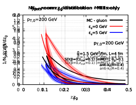
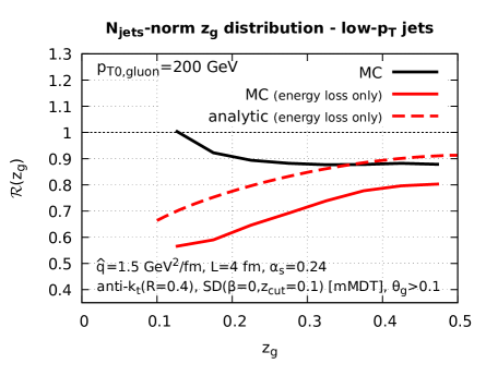
Figure 15: Separation of the nuclear effects on the $z_{g}$ distribution of low-energy jets into a contribution due to the MIEs (left) and a contribution due to the VLEs with energy loss (right). Left: MIEs only (MC vs. analytic calculations). Right: Monte Carlo results for the full parton shower (black) vs. the case where only VLEs with energy loss are included (red). We also show an analytic result for the second case (dashed line).

In Fig. 15(left) we compare our analytic approximation for the ratio $f_{\text{med}}(z_{g})/f_{\text{vac}}(z_{g})$ of the $N_{\text{jets}}$-normalised $z_{g}$ distributions corresponding the a gluon-initiated jet to the MC results obtained by “switching off” the VLEs from the general numerical code. The energy losses are estimated from the fit to the MC results shown in the left plot of Fig. 5, which yields $\varepsilon_{\rm g}\simeq 16.5$ GeV for the whole jet with $R=0.4$ and $\bar{\varepsilon}_{\rm g}\simeq 5$ GeV for the subjet with $\theta_{g}\simeq\theta_{\text{cut}}=0.1$. Given the large uncertainty in the calculation of $\bar{\varepsilon}_{\rm g}$, we present two sets of results, one corresponding to $\varepsilon_{\rm g}=0$ GeV and the other one to $\varepsilon_{\rm g}=5$ GeV. For each of these 2 choices we indicate by a band the uncertainty associated with $\pm 10\%$ variations in the saturation scale $Q_{s}$ around its central value $Q_{s}=\sqrt{\hat{q}L}=2.4$ GeV. This variation corresponds to the fact that the relation (37) between $z_{g}$ and $\omega$ is only approximate and the associated uncertainty in the value of $\omega$ has consequences, via Eq. (36), on the angular distribution; this uncertainty was mimicked by varying $Q_{s}$.

Fig. 15(left) shows a qualitative agreement between the MC and the analytic calculations: all the curves have a visible rise at small $z_{g}$, reflecting the fact that the BDMPS-Z spectrum behaves like $z^{-3/2}$ which is more singular than the vacuum spectrum $\propto z^{-1}$. This being said, our analytic study is still too poor to quantitatively reproduce the MC results, or to discriminate between various scenarios for the energy loss. In particular, the “zero energy loss” scenario is not in clear disagreement with the MC results. This may be related to the fact that the angular distribution in Eq. (36) favours small values $z\sim z_{\text{cut}}$ which biases the distribution towards events with a smaller-than-average energy loss.

5.4.2 Low-energy jets: energy loss only

In this section, we consider the situation (opposite to the previous section) where the SD condition is triggered by a VLE. In this case, we turn off the direct contribution of the MIEs to SD, but only keep their (indirect) effect associated with incoherent energy loss of the subjets found by the SD procedure. The physical situation is similar to the high-energy case studied in Sect. 5.3 where the “direct” contribution of the MIEs to SD was negligible by definition.

To artificially remove the direct contribution of the MIEs from the MC simulations, we have enforced that all the partons generated via MIEs propagate at angles $\theta\gg R$. This obviously overestimates the jet energy loss, simply because some of the partons which would have remained within the jet are artificially moved outside. This is fine as long as we only focus on illustrating the qualitative effects of the energy loss on the $z_{g}$ distribution.

In Fig. 15(right), we compare Monte Carlo results obtained with this artificial removal of the direct contribution of MIEs (“energy loss only”, red, curve) to the full simulation (“full”, black, curve), where both VLEs and MIEs contribute directly. Fig. 15(right) also shows the prediction of an analytic calculation which ignores the direct contribution of the MIEs to SD. This calculation is the same as the one presented in Sect. 5.3 for the case of a high-energy jet, i.e. it is based on Eqs. (29), (24) and (31), now applied to $p_{T}\simeq p_{T,0}=200$ GeV. The respective Sudakov factor is plotted in the right plot of Fig. 14. By inspection of these curves, we first notice that the effect of energy loss alone is the same for low-energy jets as it was for high-energy jets: it leads to a strong nuclear suppression of the $z_{g}$ distribution with larger effects at small $z_{g}$. Second, adding the direct contribution of the MIEs changes the picture significantly: the medium/vacuum ratio is now decreasing with $z_{g}$ and the ratio even becomes larger than one at small $z_{g}$. The difference between the two curves is, at least qualitatively, consistent with an additional peak at small $z_{g}$ from MIEs (see e.g. Fig. 15, left).

5.4.3 Low-energy jets: full parton showers

Now that we have studied both effects separately, we can provide an analytic calculation for the complete $z_{g}$ distribution for a low-energy jet, including both VLEs and MIEs.

Due to angular ordering, VLEs selected by the SD procedure are necessarily primary gluon emissions from the leading parton. However, whenever SD selects a MIE with energy fraction $z$ and emission angle $\theta_{g}$, this emission can be emitted by any of the partonic sources created via VLEs with energy $\omega>zp_{T0}$. Since, by definition, SD selects the largest-angle emission with $z_{g}$ above $z_{\text{cut}}$, these sources of MIE can have any angle in the range $\theta_{c}<\theta<\theta_{g}$. Such emissions are formally clustered by the C/A algorithm together with the subjet corresponding to the leading parton.

The $z_{g}$ distribution for a full parton shower generated by a parton of type $i=(\text{q,\,g})$ is obtained by incoherently summing up the probabilities for SD to select either a VLE or a MIE:

$$f_{i}(z_{g}) =\int_{\theta_{\text{cut}}}^{R}{\rm d}\theta_{g}\,\Delta_{i}^{\text{VLE}}(R,\theta_{g})\,\Delta_{i}^{\text{MIE}}(R,\theta_{g})$$ (40)

$$\times\int_{0}^{1/2}{\rm d}z\Big{[}\mathcal{P}_{i,\text{vac}}(z,\theta_{g})\delta\big{(}\mathcal{Z}_{g,\text{vac}}(z,\theta_{g})-z_{g}\big{)}+\mathcal{P}_{i,\text{med}}(z,\theta_{g})\delta\big{(}\mathcal{Z}_{g,\text{med}}(z,\theta_{g})-z_{g}\big{)}\Big{]}\Theta(z_{g}-z_{\text{cut}}).$$

Here, we have used different functions, $\mathcal{Z}_{g,\text{vac}}(z,\theta_{g})$ and $\mathcal{Z}_{g,\text{med}}(z,\theta_{g})$, for the relation between the measured splitting fraction $z_{g}$ and the physical one $z$, to take into account the fact that the energy loss is generally different for the subjets produced by a VLE or a MIE. The function $\mathcal{Z}_{g,\text{vac}}(z,\theta_{g})$ is given by Eq. (29), with the $p_{T}$ of the parent gluon identified with the $p_{T0}$ of the leading parton. As before, we replace $\theta_{g}$ by $R$ in the energy loss and take $\mathcal{E}_{1}(zp_{T},R)$ and $\mathcal{E}_{2}((1-z)p_{T},R)$ from the fits in Fig. 4. In the case of a medium-induced splitting, we use a generalisation of Eq. (37), that is

$$z_{g}\,\simeq\,\frac{zp_{T0}-\bar{\varepsilon}_{\rm g}(\theta_{g})}{p_{T0}-\mathcal{E}_{i}(p_{T0},R,z_{g})}\,\equiv\mathcal{Z}_{g,\text{med}}(z,\theta_{g})\,.$$ (41)

The main difference w.r.t. Eq. (37) refers to the energy loss by the whole jet, i.e. the function $\mathcal{E}_{i}(p_{T0},R,z_{g})$ in the denominator: not only this has now a strong dependence upon $p_{T0}$, due to the rise in the number of partonic sources via VLEs, but this must be evaluated for the special jets which include a hard splitting with a given value $z_{g}>0.1$ and with any $\theta_{g}>\theta_{\text{cut}}=0.1$. From our MC calculation illustrated in Fig. 10, we know that it is larger than the average energy loss and largely independent of $z_{g}$. We use $\mathcal{E}_{\text{g}}=43$ GeV for $p_{T0}=200$ GeV and $R=0.4$. As for $\bar{\varepsilon}_{\text{g}}(\theta_{g})$, we use 5 GeV as in Sect. 5.4.1 and study the sensitivity of our results to variations around this value.

The vacuum splitting probability density $\mathcal{P}_{i,\text{vac}}$ and the associated Sudakov factor $\Delta_{i}^{\text{VLE}}$ take the same form as in Sect. 5.3, Eqs. (24) and (31). The corresponding medium-induced probability density $\mathcal{P}_{i,\text{med}}$ takes a form similar to Eq. (35) modified to account for the fact that each VLE produced in the medium can act as a source of MIE. We therefore write

$$\mathcal{P}_{i,\text{med}}(z,\theta_{g}) =\nu(z,\theta_{g})\,\frac{\alpha_{s,\text{med}}C_{i}}{\pi}\sqrt{\frac{2\omega_{\rm c}}{p_{T0}}}\,z^{-3/2}\,\mathcal{P}_{\text{broad}}(z,\theta_{g}).$$ (42)

The number of MIE sources $\nu(z,\theta_{g})$ is obtained from the density $\tfrac{{\rm d}^{2}N_{\text{VLE}}^{\text{(in)}}}{{\rm d}\omega{\rm d}\theta}$ of VLEs produced inside the medium:

$$\nu(z,\theta_{g})\equiv 1+\int_{zp_{T0}}^{p_{T0}}{\rm d}\omega\int_{\theta_{c}}^{\theta_{g}}{\rm d}\theta\frac{{\rm d}^{2}N_{\text{VLE}}^{\text{(in)}}}{{\rm d}\omega{\rm d}\theta}\,.$$ (43)

In this last expression, the first term corresponds to the leading parton and the integration boundaries in the second term impose that an MIE which triggers the SD condition has to come from a source of larger energy at an angle between $\theta_{c}$ and $\theta_{g}$. The associated Sudakov factor $\Delta_{i}^{\text{MIE}}$ is then constructed in terms of $\mathcal{P}_{i,\text{med}}$ as in Eq. (39). We note however that, although for the case with only MIEs, the exponentiation of the emission probability in the Sudakov factor $\Delta_{i}^{\text{MIE}}$ is relatively straightforward, this does not obviously hold in the presence of multiple sources of MIEs. However, since the Sudakov factor $\Delta_{i}^{\text{MIE}}$ only introduces a small correction (see Fig. 14, right), we have kept the exponential form, Eq. (39), for simplicity and as an easy way to maintain the conservation of probability for MIEs.

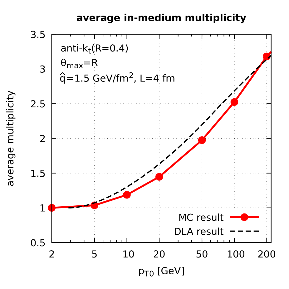
Figure 16: The average multiplicity of partons created inside the medium via VLEs by a leading gluon with $p_{T0}=200$ GeV: the full Monte Carlo results shown by (red) points are compared with a running-coupling extension of the DLA estimate in Eq. (5), integrated over the “inside” region of the phase-space of Fig. 1.

In practice, we test three different approximations for $\nu$: (i) $\nu\equiv\nu_{\rm min}=1$ includes only the leading parton, (ii) $\nu\equiv\nu_{\rm max}=3.2$ is our MC estimate for the average multiplicity of partons created inside the medium via VLEs by a leading gluon with $p_{T0}=200$ GeV, cf. Fig 16. This has to be seen as a maximal value since it ignores the kinematic limits in Eq. (43)). (iii) $\nu\equiv\nu_{\rm DLA}$ obtained by evaluating Eq. (43) with a DLA estimate for the gluon multiplicity, corresponding to Eq. (5) with $\theta_{\text{max}}\to\theta_{g}$ and taking the coupling $\bar{\alpha}_{s}$ at the scale $k_{\perp}=E\theta_{g}$. We see in Fig. 16 that this DLA approximation gives a reasonable description of the VLE multiplicity in a jet (setting $\theta_{g}=R$). For the case $\nu=\nu_{\rm DLA}$ we show no variation band in Fig. 17 to avoid overlapping bands in an already complicated plot, but it is quite clear what should be the effects of varying $\bar{\varepsilon}_{\rm g}$ and $Q_{s}^{2}$.

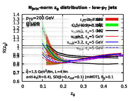
Figure 17: $\mathcal{R}(z_{g})$ for a leading parton (left: gluon, right: quark) with initial transverse momentum $p_{T0}=200$ GeV. The Monte Carlo results are compared to analytic calculations corresponding to 3 different approximations for the number $\nu$ of sources emitting MIEs (see the text for details).

In Fig. 17, we show our MC results for a full shower generated by a leading parton, gluon (left) or quark (right), with $p_{T0}=200$ GeV, together with our analytic approximation based on Eq. (40) using the three different approximations for $\nu$. In each case, the central curve corresponds to the average values $\bar{\varepsilon}_{\text{g}}=5$ GeV for the subjet energy loss in Eq. (41) and $Q_{s}^{2}=\hat{q}L=6$ GeV² for the saturation momentum squared in (36). The bands around these central curves correspond to variations by 20% of $\varepsilon_{\rm g}$. Note that varying $Q_{s}^{2}$ by 20% has a smaller effect. The unphysical case $\nu_{\rm min}=1$ is disfavoured by the comparison with the MC results as it underestimates the peak associated with the direct MIE contribution. The other two cases are at least qualitatively consistent with the MC results.

It is also interesting to notice the dependence of the results upon the flavour of the leading parton. The rise of the nuclear distribution at small $z_{g}$ appears to be stronger for the gluon-initiated jet than for the quark-initiated one and this difference is rather well captured by our analytic approximations, where it is due to a change in the number $\nu$ of partonic sources for a “hard” MIE: one has indeed $\nu-1\propto C_{R}$ (recall e.g. the discussion in footnote 10). At large $z_{g}$ on the other hand, the analytic approximation appears to be less satisfactory for the quark-initiated jet — most likely, because it underestimates the energy loss by the subjets resulting from a hard VLE. As a matter of facts, a similar difficulty occurs in the high-energy case, as can be seen by comparing the quark-jet results for $p_{T0}=1$ TeV in Figs. 8 and 13 respectively.

The main conclusions that we can draw from in Fig. 17 and from the overall discussion in this section is that $z_{g}$ distribution for “low energy jets” is a superposition of two main effects: (i) incoherent energy loss for the subjets created by a vacuum-like splitting; this controls the $z_{g}$ distribution at moderate and large values of $z_{g}$, where it yields a nuclear modification factor which slowly increase with $z_{g}$, and (ii) sufficiently hard medium-induced emissions, with $z\gtrsim z_{\text{cut}}$, which leads to a significant growth of the $z_{g}$ distribution at small values $z_{g}\sim z_{\text{cut}}$. This behaviour is qualitatively reproduced by our simple analytic calculations which shows, for example, that including multiple (VLE) sources of MIEs is important. It is however more delicate to draw more quantitative conclusions as several effects entering the calculation would require a more involve treatment.

6 $z_{g}$ distribution with realistic initial jet spectra

Even if studying monochromatic jets is helpful to understand the dominant physical effects at play, any realistic measurement would instead impose cuts on the $p_{T,{\rm jet}}\equiv p_{T}$ of the final jet. For this we need the full $p_{T0}$ spectrum of the hard scattering. Here, we follow our prescription from Section 4.2 and use a LO dijet spectrum where both final partons are showered using our Monte Carlo. One can then cluster and analyse the resulting event.

In the case of the $z_{g}$ distribution, it is interesting to note that we expect a competition between two effects. On one side, due to the steeply-falling underlying $p_{T0}$ spectrum, cutting on the jet $p_{T}$ tends to select jets which lose less energy than average. On the other side, we have seen from Fig. 10 that jets with $z_{g}>z_{\text{cut}}$ and $\theta_{g}>\theta_{\text{cut}}$ lose more energy than average.

Below, we first study the case of the $N_{\text{jets}}$-normalised $z_{g}$ distribution which is best suited to discuss the underlying physical details highlighted in section 5. Our distributions are also qualitatively compared to a recent experimental analysis by ALICE Acharya:2019djg . We then consider the self-normalised $z_{g}$ distribution which is more easily compared to the CMS measurements Sirunyan:2017bsd .

6.1 Phenomenology with the $N_{\text{jets}}$-normalised $z_{g}$

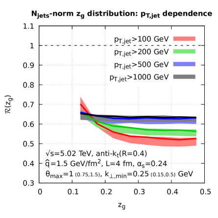
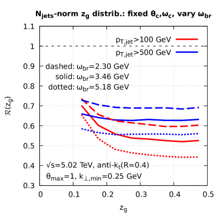
Figure 18: Our full MC predictions for the medium/vacuum ratio $\mathcal{R}(z_{g})$ of the $N_{\text{jets}}$-normalised $z_{g}$ distributions, including the convolution with the initial jet spectrum. Left: the sensitivity of our results to changes in the kinematic cuts $\theta_{\rm max}$ and $k_{\perp,\text{min}}$. Right: the effect of varying $\omega_{\rm br}$ (by $\pm 50\%$) at fixed values for $\omega_{\rm c}$ and $\theta_{c}$.

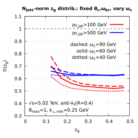
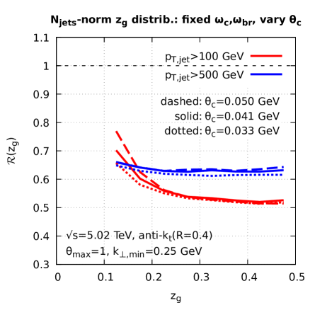
Figure 19: The effects of varying $\hat{q}$, $L$ and ${\alpha}_{s,\text{med}}$ keeping $\omega_{\rm br}=3.46$ GeV fixed at its central value (cf. the right plot of Fig. 6). Left: we vary $\omega_{\rm c}$ by $\pm 50\%$ at fixed $\theta_{c}$. Right: we vary $\theta_{c}^{2}$ by $\pm 50\%$ at fixed $\omega_{\rm c}$.

Our main results for the $N_{\text{jets}}$-normalised $z_{g}$ distribution are plotted in Figs. 18–19. They are the analog of the results for $R_{AA}$ shown in Figs. 6–7: they highlight the $p_{T}$-dependence of our predictions together as well as their sensitivity to changes in the physical ($\hat{q}$, $L$ and ${\alpha}_{s,\text{med}}$) and unphysical ($\theta_{\rm max}$ and $k_{\perp,\text{min}}$) parameters. The various curves shown in these figures have been obtained by integrating the $z_{g}$ distribution over all the values of $p_{T}$ above a lower cutoff $p_{T,{\rm min}}$ (explicitly shown for each curve). In practice, our choices for this cutoff are the same as the values taken for $p_{T0}$ in Fig. 8. Since the jet $p_{T}$ spectrum falls rapidly with $p_{T}$ and the jet energy loss is relatively small compared to the jet $p_{T}$, it makes sense to compare the respective results.

First of all, we see from Fig. 18, left, that our predictions are robust w.r.t. variations of the unphysical parameters in our Monte Carlo. Then, based on the analyses from section 5, we expect the $z_{g}$ distribution to be mostly sensitive to changes in the multiple-branching energy scale $\omega_{\rm br}$ which controls both the energy loss and the rate for SD to be triggered by a MIE. When varying $\omega_{\rm br}$ by 50% around its central value, keeping $\omega_{\rm c}$ and $\theta_{c}$ fixed, the $z_{g}$ distribution is indeed strongly affected, see Fig. 18, right. The effects of changing either $\omega_{\rm c}$ or $\theta_{c}$, at fixed $\omega_{\rm br}$, are much less pronounced as seen in Fig. 19. The residual variations observed when varying $\omega_{\rm c}$ or $\theta_{c}$ can be mainly attributed to variations in the phase-space for VLEs, which affect the multiplicity of sources for MIEs and the energy loss (cf. Eq. (42)). Besides, for the low-$p_{T}$ jets, a change in $\omega_{\rm c}$ can have a sizeable effect on the phase-space for MIEs that are accessible to SD (cf. Fig. 9). This is indeed seen in Fig. 19 which shows a stronger dependence on $\omega_{\rm c}$ than on $\theta_{c}$, especially for the peak at low $p_{T}$ and small $z_{g}$.

Comparing now to the results for monochromatic jets shown in Fig. 8, we observe important differences that can be understood as follows. When studying the $N_{\text{jets}}$-normalised ratio, the deviation of $\mathcal{R}(z_{g})=f_{\text{med}}(z_{g})/f_{\text{vac}}(z_{g})$ from unity is proportional to the ratio, $N_{\rm SDjets}/N_{\rm jets}$, between the number of jets which passed the SD condition and the total number of jets. This ratio is considerably smaller when using a realistic jet spectrum, Fig. 18 (left), than for monochromatic jets, Fig. 8. This is explained by the fact that jets passing the SD condition lose more energy than average jets and therefore have a more suppressed production rate. Moreover, among the jets which have passed SD with a given $z_{g}>z_{\text{cut}}$, the initial cross-section favours those where the subjets have lost less energy, leading to a flattening in the shape of the ratio $\mathcal{R}(z_{g})$ at large $z_{g}$, in agreement with Fig. 18 left. Finally, imposing a lower $p_{T}$ cut on jets introduces a bias towards quark jets, which lose less energy than gluon jets. Since the former have a smaller $\mathcal{R}(z_{g})$ than the latter (cf. Fig. 8), this further reduces $\mathcal{R}(z_{g})$ for jets.

Another interesting feature of Fig. 18 left is the fact that the ratio $\mathcal{R}(z_{g})$ is almost identical for $p_{T}=500$ GeV and $p_{T}=1$ TeV. We believe that this purely fortuitous. First, the normalisation factor $N_{\rm SDjets}/N_{\rm jets}$ penalises the jets with $p_{T}=1$ TeV more than those with $p_{T}=500$ GeV, thus reducing an initially-small difference between the respective results in Fig. 8. Second, as $p_{T}$ increases so does the fraction of quark-initiated jets, thus contributing to a reduction of $\mathcal{R}(z_{g})$.

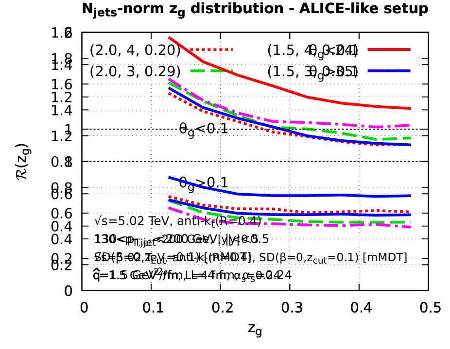
Figure 20: Predictions of our Monte Carlo generator for the $z_{g}$ distribution obtained with a setup similar to the one used in the ALICE measurement of Ref.Acharya:2019djg . We included the distribution obtained with either $\theta_{g}<0.1$ (bottom set of curves), or $\theta_{g}>0.1$ (top set of curves). In each case we show the result for different sets of medium parameters, $\hat{q}$, $L$ and $\alpha_{s}$ as indicated in the legend.

At this point, it is interesting to compare our predictions with the measurements by the ALICE collaboration Acharya:2019djg at the LHC. This is not immediately straightforward as the ALICE measurement is at a different collider energy than what we have considered so far, uses only charged tracks which are not accessible in our parton-level shower, and is not unfolded for the detector effects and residual background fluctuations. For simplicity, we keep the collider energy at 5.02 TeV. Since the charged and full transverse momenta of jets are roughly proportional to one another, we scale the acceptance region for the jet $p_{T}$ from $[80,120]$ GeV to $[130,200]$ GeV and work with all the particles. The discussion below should therefore, at best, be considered as qualitative.

Our findings are presented in Fig. 20 where, following Ref. Acharya:2019djg (see the first and third plots in Fig. 3), we have considered both the case $\theta_{g}>0.1$ and the case $\theta_{g}<0.1$. Our predictions are shown for a range of medium parameters (see also Table 1 of Fig. 21). In all cases, our results are qualitatively similar to those of the experimental analysis: the ratio $\mathcal{R}(z_{g})$ is decreasing with $z_{g}$, it shows nuclear suppression ($\mathcal{R}(z_{g})<1$) for the large-angle case $\theta_{g}>0.1$ and nuclear enhancement ($\mathcal{R}(z_{g})>1$) for the small-angle case $\theta_{g}<0.1$. Within our framework, the enhancement observed for $\theta_{g}<0.1$ and the rise at small $z_{g}$ are both associated with medium-induced emissions being captured by SD. The suppression visible for $\theta_{g}>0.1$ is a consequence of incoherent energy loss as seen in Sect. 5.

6.2 Self-normalised $z_{g}$ distribution and CMS data

We want to compare the predictions of our Monte Carlo generator to the measurement of the self-normalised $z_{g}$ distribution by the CMS collaboration in Ref. Sirunyan:2017bsd . This comparison should however be taken with care since the CMS results are not unfolded for detector (and residual Underlying Event) effects and are instead presented under the form of “PbPb/smeared pp” ratios. Without a proper dedicated study, it is delicate to assess the precise effects of this smearing on $\mathcal{R}^{\text{(norm)}}(z_{g})$.

$\hat{q}$	$L$	$\alpha_{s}$	$\theta_{c}$	$\omega_{c}$	$\omega_{\text{br}}$
1.5	3	0.35	0.0629	33.75	4.134
1.5	4	0.24	0.0408	60	3.456
2	3	0.29	0.0544	45	3.784
2	4	0.2	0.0354	80	3.200

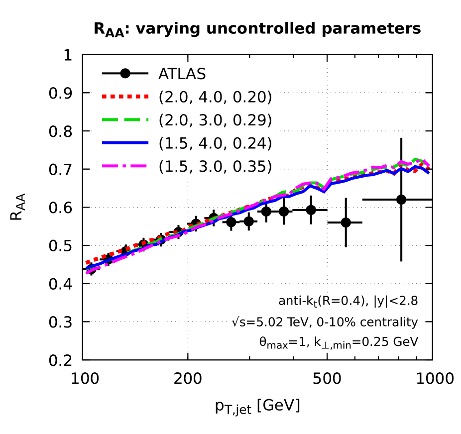
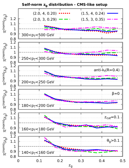
Figure 21: Left: our MC results for jet $R_{AA}$ and for 4 sets of medium parameters which give quasi-identical predictions are compared to the ATLAS data Aaboud:2018twu (black dots with error bars). Right: the MC predictions for the medium/vacuum ratio $\mathcal{R}^{\text{(norm)}}(z_{g})$ of the self-normalised $z_{g}$ distributions are presented in bins of $p_{T}$ for the same 4 sets of medium parameters as in the left figure.

Our findings are shown in Fig. 21(right). In the left plot, we show a selection of 4 sets of medium parameters, $\hat{q}$, $L$ and ${\alpha}_{s,\text{med}}$ (reported from Table 1 for readability) which provide a good description of the LHC data Aaboud:2018twu for the jet $R_{AA}$ ratio. In the right plot, we show the corresponding predictions for the $z_{g}$ nuclear modification factor, $\mathcal{R}^{\text{(norm)}}(z_{g})$, using the same bins and cuts as in the CMS analysis.

We see that our 4 choices of medium parameters correspond to somewhat different values for the physical medium scales $\omega_{\rm br}$, $\omega_{\rm c}$ and $\theta_{c}$. They therefore lead to different predictions both for the average energy lost by a single parton at large angles, dominated by $\omega_{\rm br}$, and for the number and distribution of sources, which is controlled via the phase-space boundaries for VLEs by $\omega_{\rm c}$ and $\theta_{c}$. While the $R_{AA}$ ratio is most sensitive to variations in $\omega_{\rm br}$, small variations in $\omega_{\rm br}$ ($\sim 30$% between our extreme values) can be compensated by larger variations of $\omega_{\rm c}$ and $\theta_{c}$ (a factor $\sim 2$ between our extreme values). Since the interplay between the 3 scales $\omega_{\rm br}$, $\omega_{\rm c}$ and $\theta_{c}$ is different for $R_{AA}$ and $\mathcal{R}^{\text{(norm)}}(z_{g})$, our 4 sets of parameters predict different behaviours for the latter. However, both observables are predominantly controlled by the energy loss of the jet, so the spread in $\mathcal{R}^{\text{(norm)}}(z_{g})$ remains limited. Some differences are nonetheless observable, in particular for the two bins with the largest $p_{T}$. The predictions obtained with a larger $\omega_{\rm br}$ — i.e. larger single-parton energy loss but smaller phase-space for VLEs — show a pattern dominated by energy loss, similar to what was seen in Sect. 5 for high-$p_{T}$ jets. Conversely, the predictions obtained with a smaller $\omega_{\rm br}$ — i.e. smaller single-parton energy loss but larger phase-space for VLEs — show an enhancement of the small-$z_{g}$ peak associated to MIEs.

If we compare these results with the CMS measurements (see e.g. Fig. 4 of Ref. Sirunyan:2017bsd ), we see that the two agree within the error bars for both the pattern and the magnitude of the deviation from one. In particular, the CMS data too indicate that $\mathcal{R}^{\text{(norm)}}$ decreases quasi-monotonously with $z_{g}$ at low $p_{T}$ and become flatter and flatter, approaching unity, when increasing $p_{T}$. This supports our main picture where the nuclear effects on the $z_{g}$ distribution are a combination of incoherent energy loss affecting a vacuum-like splitting and a small-$z_{g}$ peak associated with the SD condition being triggered by a MIE. With increasing $p_{T}$ the first mechanism dominates over the over, yielding a flatter distribution, in agreement with the CMS data. That being said, the current experimental uncertainty does not allow one to distinguish between different sets of medium parameters.

6.3 Substructure observables beyond the $z_{g}$ distribution

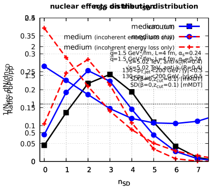
Figure 22: $n_{\text{SD}}$ distributions emerging from our Monte Carlo simulations. Left: the distributions themselves, for the vacuum shower, for the full in-medium parton shower, and also for the case where the MIEs contribute only to the energy loss (but not directly to SD). Right: the medium/vacuum ratios.

Our final section discusses two substructure observables related to the $z_{g}$ distribution.

Iterated SD multiplicity.

The first observable we consider is the Iterated SD multiplicity Frye:2017yrw , $n_{\text{SD}}$, which has also been measured on track-jets by the ALICE collaboration Acharya:2019djg . Iterated SD proceeds by iterating the Soft-Drop procedure, still following the hardest branch in the jet, until all declusterings have been exhausted. $n_{\text{SD}}$ is then defined as the number of declusterings passing the SD condition.

Our results for the $n_{\text{SD}}$ distribution are presented in Fig. 22 and show the same trend as the ALICE measurements (Fig. 4 of Ref. Acharya:2019djg ). In particular, the $n_{\rm SD}$ distribution is shifted to smaller values for jets created in PbPb collisions compared to pp collisions. This might seem puzzling at first sight since in the low-$p_{T,\text{jet}}$ range probed by the measurement, one could naively expect an enhancement of $n_{\rm SD}$ due to the additional MIEs passing the SD condition. However, we believe that the dominant mechanism at play is the incoherent energy loss which, as discussed in Sect. 5.3, results in an effective $z_{g}$ fraction smaller than the actual momentum fraction $z$ at the splitting. This effect lowers the number of measured hard splittings. To support this argument, we have run a variant of our MC simulations where all the partons created via MIEs are moved outside the jet and hence only they only contribute to the energy loss. The corresponding results, shown as crosses in Fig. 22 demonstrate as expected an even stronger reduction in the average value of $n_{\rm SD}$, which is only partially compensated by MIEs captured by the Iterated SD procedure.

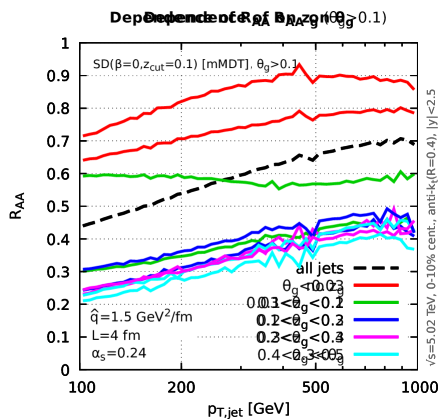
Figure 23: Our MC results for the jet $R_{AA}$ as a function of $p_{T,{\rm jet}}$ are shown in bins of $z_{g}$ (left figure) and in bins of $\theta_{g}$ (right figure). The inclusive (all-$z_{g}$, respectively all-$\theta_{g}$) results are shown with dashed lines.

Correlation between $R_{AA}$ and $z_{g}$.

Given that both $R_{AA}$ and the $z_{g}$ distribution are primarily controlled by the jet energy loss, it is interesting to study the correlation between these 2 variables (similarly to Fig. 10 for the energy loss of monochromatic jets). To that aim, we show in Fig. 23 the ratio $R_{AA}$ as a function of $p_{T}\equiv p_{T,{\rm jet}}$ for different bins in $z_{g}$ (imposing $\theta_{g}>0.1$) (left plot) and for different bins in $\theta_{g}$ (right plot). For reference, the inclusive $R_{AA}$ ratio is shown by the “all jets” curve. The curve labelled as “no $z_{g}$” in the left plot includes both the events which did not pass the SD criteria and the events which failed the $\theta_{g}>0.1$ constraint. Correspondingly, the curve labelled “$\theta_{g}<0.03$” in the right plot includes both the events with a genuine splitting passing the SD condition with $\theta_{g}<0.03$ and the events which did not pass the SD condition.

The remarkable feature in both plots is the striking difference between the events which passed SD and those which did not. As explained when we discussed Fig. 10, this difference reflects the fact that, on average, two-prong jets lose more energy than single-prong ones. These results also reveal the role played by colour (de)coherence and the emergence of a critical angle $\theta_{c}$. With our choice of parameters, $\theta_{c}\simeq 0.04$ corresponds to the region in $\theta_{g}$ where $R_{AA}$ changes significantly. For example, the curve corresponding to $\theta_{g}<0.03<\theta_{c}$ receives almost exclusively contributions from single-prong jets — even more so than the “no $z_{g}$ curve in the left plot — and thus shows a nuclear factor $R_{AA}$ close to unity. This suggests that measuring $R_{AA}$ in bins of $\theta_{g}$ can be interesting to better characterise the propagation of jets in the quark-gluon plasma.

7 Conclusions and perspectives

In this paper, we have presented a new picture, emerging from perturbative QCD, for the parton shower created by an energetic parton propagating through a dense quark-gluon plasma. This picture is factorised in time with vacuum-like emissions occurring first and creating sources for subsequent medium-induced radiation. Both types of emission are Markovian processes, yielding a modular Monte Carlo implementation of our picture. This allows us to study separately various aspects of the dynamics of jet quenching and assert their relative importance. In practice, we have focused on two observables for which we believe our approximations to be robust: the jet nuclear modification factor for $R_{AA}$ and the nuclear effects on the $z_{g}$ distribution given by the Soft Drop procedure.

For both observables, we obtained good qualitative and semi-quantitative descriptions of the respective LHC data and we discussed the physical interpretation of the various trends seen in the data. To make our physical discussions more convincing, we supplemented the numerical calculations of the $z_{g}$ distribution with suitable analytic calculations, which were helpful to pinpoint the different mechanisms at play and compare their effects. Our formalism involves a few free parameters, notably $\hat{q}$ and $L$, but we have checked that the quality of our description of the data depends on these parameters only via microscopic scales built with these parameters. In particular, the energy scale $\omega_{\rm br}\sim\alpha_{s}^{2}\hat{q}L^{2}$ controls the energy loss via soft medium-induced emissions at large angles.

We found that these two observables are to a large extent controlled by the jet energy loss. They are therefore very sensitive both to vacuum-like emissions (which drive the number of sources for medium-induced radiation) and to medium-induced emissions. In particular, the increase of the number of vacuum-like emissions with the jet $p_{T}$ causes an increase in the jet energy loss.

We showed that the nuclear $z_{g}$ distribution is affected by both a direct contribution of the MIEs and their indirect contribution, via the incoherent energy loss of the two subjets selected by the SD procedure. The former leads to a pronounced rise of the $z_{g}$ distribution at small $z_{g}$, as seen in the data. The latter causes a nuclear suppression ($\mathcal{R}(z_{g})<1$ and slowly increasing with $z_{g}$), which is best seen when normalising the $z_{g}$ distribution to the total number of jets (the $N_{\text{jets}}$-normalised distributions in our nomenclature). The interplay between the two effects depends on the jet $p_{T}$. At low $p_{T}$, $p_{T}\lesssim 300$ GeV, corresponding to the current range covered by the LHC analyses, both effects contribute. As the jet $p_{T}$ increases, MIEs become too soft to trigger the SD condition and only the indirect effect of (incoherent) energy loss survives. As a consequence, we predict that for $p_{T}\gtrsim 500$ GeV, the ($N_{\text{jets}}$-normalised) nuclear modification factor $\mathcal{R}(z_{g})$ should be systematically smaller than one and slowly increasing with $z_{g}$. The onset of such a transition is consistent with the largest $p_{T}$ bin of the CMS measurement.

Some of our results have been anticipated by previous studies in the literature, with somewhat different conclusions. When studying the consequences of the incoherent energy loss on the $z_{g}$ distribution, Refs. Mehtar-Tani:2016aco ; Chang:2017gkt obtained results which are qualitatively similar to the curve denoted as “energy loss only” in our Fig. 15, right, i.e. $\mathcal{R}(z_{g})<1$ with an increase with $z_{g}$. This trend is opposite to the one seen in the LHC data at $p_{T}\lesssim 250$ GeV Sirunyan:2017bsd , which led Refs. Mehtar-Tani:2016aco ; Chang:2017gkt to argue that the LHC data favours a scenario of coherent energy loss by the two subjets. Such a conclusion seems difficult to reconcile with the fact that, in the CMS analysis Sirunyan:2017bsd , the angular separation $\theta_{g}$ between the two subjets is constrained to values $\theta_{g}\geq\theta_{\text{cut}}=0.1$ which, with our current estimates, are considerably larger than the critical angle $\theta_{c}$ for the onset of colour decoherence. In our picture, we instead conclude that the rise of the $z_{g}$ distribution at small $z_{g}$ is due to the relatively hard MIEs that can be captured by SD and which more than compensate the suppression due to the incoherent energy loss. This is indeed visible for our full Monte Carlo results in Fig. 15, right. This shows the importance of having a complete physical picture and the usefulness of the corresponding numerical implementation.

In the remaining part of these conclusions, we emphasise the limitations of our current approach and thus outline some of our projects for the future. Even though we describe the parton showers from first principles, our current treatment of the medium — a homogeneous “brick” of quark-gluon plasma — is insufficient for more detailed phenomenological studies. Besides our implementation of an angular-ordered final-state parton shower can be significantly refined.

A first step towards a more realistic description of the medium is to include its longitudinal expansion, e.g. by giving a suitable time-dependence to the jet quenching parameter $\hat{q}$ Baier:1998yf ; Zakharov:1998wq ; Arnold:2008iy ; Iancu:2018trm . One would also need a more realistic geometry (say, an expanding cylinder for central collisions) together with a probability distribution for the location of the hard process inside the medium. Further refinements would also include the radial expansion and a fully dynamical description of the plasma, including its response to the jet. The current belief is that the inclusion of the medium backreaction is important for observables like the jet shapes Chatrchyan:2013kwa and the geometrical distribution of the energy lost by the jet, e.g. as measured by the dijet asymmetry Aad:2010bu ; Chatrchyan:2011sx ; Khachatryan:2016erx .

Several other improvements of the medium-induced cascade can be implemented. First, we should relax the fixed coupling approximation in the treatment of the medium-induced radiation. Second, one should use a dynamic treatment of the transverse momentum broadening, which explicitly includes the elastic collisions and thus goes beyond our current Gaussian approximation. In practice, hard collisions would generate a power-law tail $\propto k_{\perp}^{-4}$ at large $k_{\perp}$. This can have a sizeable impact on the $z_{g}$ distribution which, as discussed in Sect. 5.4.1, is sensitive to the large-$k_{\perp}$ tail of the $k_{\perp}$ distribution. A Monte Carlo implementation of the elastic collisions (in the diffusion approximation) has recently been presented Kutak:2018dim for a jet evolving via (BDMPS-Z) medium-induced radiation alone. In the future, we plan to extend the method in Kutak:2018dim to the full parton shower, including VLEs. More generally, one could also add the effects of elastic collisions in terms of energy loss (the “drag force”) and longitudinal momentum broadening. This would be important for the in-medium dynamics of the softest quanta from the jet, in particular for the possibility of their thermalisation Baier:2000sb ; Kurkela:2015qoa ; Iancu:2015uja .

Finally, our vacuum parton shower should be extended to include the single-logarithmic effects of soft gluon emissions beyond the collinear limit, and to include both final-state and initial-state radiation. This can e.g. be done using a dipole shower which would also have the advantage of facilitating the interface of our parton shower with hadronisation models.

Instead of going through the complex task of completing our Monte Carlo with a detailed description of the medium and of its interactions with the jet, one can alternatively think about using our parton showers as an input for the recently developed JETSCAPE Cao:2017zih ; Putschke:2019yrg framework, which offers various approaches for treating the interactions between the parton shower and the medium. Last but not least, it would be both important and instructive to understand in detail the relation between our approach and the related approaches in the literature, notably those used by the Monte Carlo event generators MARTINI Schenke:2009gb and JEWEL Zapp:2011ya ; Zapp:2012ak , which share with us the fact that both the parton showers and the in-medium interactions are treated in perturbative QCD.

References

- (1) Y. Mehtar-Tani, J. G. Milhano, and K. Tywoniuk, “Jet physics in heavy-ion collisions,” Int.J.Mod.Phys. A28 (2013) 1340013, arXiv:1302.2579 [hep-ph].
- (2) J.-P. Blaizot and Y. Mehtar-Tani, “Jet Structure in Heavy Ion Collisions,” Int. J. Mod. Phys. E24 no. 11, (2015) 1530012, arXiv:1503.05958 [hep-ph].
- (3) G.-Y. Qin and X.-N. Wang, “Jet quenching in high-energy heavy-ion collisions,” Int. J. Mod. Phys. E24 no. 11, (2015) 1530014, arXiv:1511.00790 [hep-ph]. [,309(2016)].
- (4) H. A. Andrews et al., “Novel tools and observables for jet physics in heavy-ion collisions,” arXiv:1808.03689 [hep-ph].
- (5) A. J. Larkoski, S. Marzani, and J. Thaler, “Sudakov Safety in Perturbative QCD,” Phys. Rev. D91 no. 11, (2015) 111501, arXiv:1502.01719 [hep-ph].
- (6) A. J. Larkoski, S. Marzani, G. Soyez, and J. Thaler, “Soft Drop,” JHEP 05 (2014) 146, arXiv:1402.2657 [hep-ph].
- (7) CMS Collaboration, A. M. Sirunyan et al., “Measurement of the Splitting Function in and Pb-Pb Collisions at 5.02 TeV,” Phys. Rev. Lett. 120 no. 14, (2018) 142302, arXiv:1708.09429 [nucl-ex].
- (8) ALICE Collaboration, S. Acharya et al., “Exploration of jet substructure using iterative declustering in pp and Pb-Pb collisions at LHC energies,” arXiv:1905.02512 [nucl-ex].
- (9) Y.-T. Chien and I. Vitev, “Probing the Hardest Branching within Jets in Heavy-Ion Collisions,” Phys. Rev. Lett. 119 no. 11, (2017) 112301, arXiv:1608.07283 [hep-ph].
- (10) Y. Mehtar-Tani and K. Tywoniuk, “Groomed jets in heavy-ion collisions: sensitivity to medium-induced bremsstrahlung,” JHEP 04 (2017) 125, arXiv:1610.08930 [hep-ph].
- (11) N.-B. Chang, S. Cao, and G.-Y. Qin, “Probing medium-induced jet splitting and energy loss in heavy-ion collisions,” Phys. Lett. B781 (2018) 423–432, arXiv:1707.03767 [hep-ph].
- (12) G. Milhano, U. A. Wiedemann, and K. C. Zapp, “Sensitivity of jet substructure to jet-induced medium response,” Phys. Lett. B779 (2018) 409–413, arXiv:1707.04142 [hep-ph].
- (13) Y. L. Dokshitzer, G. D. Leder, S. Moretti, and B. R. Webber, “Better jet clustering algorithms,” JHEP 08 (1997) 001, arXiv:hep-ph/9707323 [hep-ph].
- (14) M. Wobisch and T. Wengler, “Hadronization corrections to jet cross-sections in deep inelastic scattering,” in Monte Carlo generators for HERA physics. Proceedings, Workshop, Hamburg, Germany, 1998-1999, pp. 270–279. 1998. arXiv:hep-ph/9907280 [hep-ph].
- (15) Y. L. Dokshitzer, V. A. Khoze, A. H. Mueller, and S. I. Troian, “Basics of perturbative QCD,”. Gif-sur-Yvette, France. Ed. Frontieres (1991) 274 p.
- (16) R. Baier, Y. L. Dokshitzer, A. H. Mueller, S. Peigne, and D. Schiff, “Radiative Energy Loss of High Energy Quarks and Gluons in a Finite-Volume Quark-Gluon Plasma,” Nucl. Phys. B483 (1997) 291–320, arXiv:hep-ph/9607355.
- (17) R. Baier, Y. L. Dokshitzer, A. H. Mueller, S. Peigne, and D. Schiff, “Radiative Energy Loss and P(T)-Broadening of High Energy Partons in Nuclei,” Nucl. Phys. B484 (1997) 265–282, arXiv:hep-ph/9608322.
- (18) B. G. Zakharov, “Fully Quantum Treatment of the Landau-Pomeranchuk-Migdal Effect in QED and QCD,” JETP Lett. 63 (1996) 952–957, arXiv:hep-ph/9607440.
- (19) B. G. Zakharov, “Radiative Energy Loss of High Energy Quarks in Finite-Size Nuclear Matter and Quark-Gluon Plasma,” JETP Lett. 65 (1997) 615–620, arXiv:hep-ph/9704255.
- (20) R. Baier, Y. L. Dokshitzer, A. H. Mueller, and D. Schiff, “Medium-Induced Radiative Energy Loss: Equivalence Between the Bdmps and Zakharov Formalisms,” Nucl. Phys. B531 (1998) 403–425, arXiv:hep-ph/9804212.
- (21) Y. Mehtar-Tani, C. A. Salgado, and K. Tywoniuk, “Antiangular Ordering of Gluon Radiation in QCD Media,” Phys. Rev. Lett. 106 (2011) 122002, arXiv:1009.2965 [hep-ph].
- (22) Y. Mehtar-Tani, C. A. Salgado, and K. Tywoniuk, “Jets in QCD Media: from Color Coherence to Decoherence,” Phys. Lett. B707 (2012) 156–159, arXiv:1102.4317 [hep-ph].
- (23) J. Casalderrey-Solana and E. Iancu, “Interference Effects in Medium-Induced Gluon Radiation,” JHEP 08 (2011) 015, arXiv:1105.1760 [hep-ph].
- (24) J.-P. Blaizot, F. Dominguez, E. Iancu, and Y. Mehtar-Tani, “Medium-induced gluon branching,” JHEP 1301 (2013) 143, arXiv:1209.4585 [hep-ph].
- (25) J.-P. Blaizot, F. Dominguez, E. Iancu, and Y. Mehtar-Tani, “Probabilistic picture for medium-induced jet evolution,” JHEP 1406 (2014) 075, arXiv:1311.5823 [hep-ph].
- (26) L. Apolinário, N. Armesto, J. G. Milhano, and C. A. Salgado, “Medium-induced gluon radiation and colour decoherence beyond the soft approximation,” JHEP 1502 (2015) 119, arXiv:1407.0599 [hep-ph].
- (27) P. Caucal, E. Iancu, A. H. Mueller, and G. Soyez, “Vacuum-like jet fragmentation in a dense QCD medium,” Phys. Rev. Lett. 120 (2018) 232001, arXiv:1801.09703 [hep-ph].
- (28) J.-P. Blaizot, E. Iancu, and Y. Mehtar-Tani, “Medium-induced QCD cascade: democratic branching and wave turbulence,” Phys.Rev.Lett. 111 (2013) 052001, arXiv:1301.6102 [hep-ph].
- (29) L. Fister and E. Iancu, “Medium-induced jet evolution: wave turbulence and energy loss,” JHEP 03 (2015) 082, arXiv:1409.2010 [hep-ph].
- (30) ATLAS Collaboration, M. Aaboud et al., “Measurement of the nuclear modification factor for inclusive jets in Pb+Pb collisions at TeV with the ATLAS detector,” Phys. Lett. B790 (2019) 108–128, arXiv:1805.05635 [nucl-ex].
- (31) STAR Collaboration, K. Kauder, “Measurement of the Shared Momentum Fraction using Jet Reconstruction in p+p and Au+Au Collisions with STAR,” Nucl. Part. Phys. Proc. 289-290 (2017) 137–140, arXiv:1703.10933 [nucl-ex].
- (32) T. Liou, A. Mueller, and B. Wu, “Radiative -broadening of high-energy quarks and gluons in QCD matter,” Nucl.Phys. A916 (2013) 102–125, arXiv:1304.7677 [hep-ph].
- (33) J.-P. Blaizot and Y. Mehtar-Tani, “Renormalization of the jet-quenching parameter,” Nucl.Phys. A929 (2014) 202–229, arXiv:1403.2323 [hep-ph].
- (34) E. Iancu, “The non-linear evolution of jet quenching,” JHEP 1410 (2014) 95, arXiv:1403.1996 [hep-ph].
- (35) Y. Mehtar-Tani, C. A. Salgado, and K. Tywoniuk, “The Radiation Pattern of a QCD Antenna in a Dilute Medium,” JHEP 04 (2012) 064, arXiv:1112.5031 [hep-ph].
- (36) P. Arnold and S. Iqbal, “The LPM effect in sequential bremsstrahlung,” JHEP 04 (2015) 070, arXiv:1501.04964 [hep-ph]. [Erratum: JHEP09,072(2016)].
- (37) P. Arnold, H.-C. Chang, and S. Iqbal, “The LPM effect in sequential bremsstrahlung 2: factorization,” JHEP 09 (2016) 078, arXiv:1605.07624 [hep-ph].
- (38) U. A. Wiedemann, “Gluon Radiation Off Hard Quarks in a Nuclear Environment: Opacity Expansion,” Nucl. Phys. B588 (2000) 303–344, arXiv:hep-ph/0005129.
- (39) U. A. Wiedemann, “Jet Quenching Versus Jet Enhancement: a Quantitative Study of the Bdmps-Z Gluon Radiation Spectrum,” Nucl. Phys. A690 (2001) 731–751, arXiv:hep-ph/0008241.
- (40) P. B. Arnold, G. D. Moore, and L. G. Yaffe, “Photon Emission from Ultrarelativistic Plasmas,” JHEP 11 (2001) 057, arXiv:hep-ph/0109064.
- (41) P. B. Arnold, G. D. Moore, and L. G. Yaffe, “Photon Emission from Quark Gluon Plasma: Complete Leading Order Results,” JHEP 12 (2001) 009, arXiv:hep-ph/0111107.
- (42) P. B. Arnold, G. D. Moore, and L. G. Yaffe, “Photon and Gluon Emission in Relativistic Plasmas,” JHEP 06 (2002) 030, arXiv:hep-ph/0204343.
- (43) Y. Mehtar-Tani and S. Schlichting, “Universal quark to gluon ratio in medium-induced parton cascade,” JHEP 09 (2018) 144, arXiv:1807.06181 [hep-ph].
- (44) E. Iancu and B. Wu, “Thermalization of mini-jets in a quark-gluon plasma,” JHEP 10 (2015) 155, arXiv:1506.07871 [hep-ph].
- (45) J.-P. Blaizot, Y. Mehtar-Tani, and M. A. C. Torres, “Angular structure of the in-medium QCD cascade,” Phys.Rev.Lett. 114 no. 22, (2015) 222002, arXiv:1407.0326 [hep-ph].
- (46) J.-P. Blaizot, L. Fister, and Y. Mehtar-Tani, “Angular distribution of medium-induced QCD cascades,” Nucl.Phys. A940 (2015) 67–88, arXiv:1409.6202 [hep-ph].
- (47) M. A. Escobedo and E. Iancu, “Event-by-event fluctuations in the medium-induced jet evolution,” JHEP 05 (2016) 008, arXiv:1601.03629 [hep-ph].
- (48) M. A. Escobedo and E. Iancu, “Multi-particle correlations and KNO scaling in the medium-induced jet evolution,” JHEP 12 (2016) 104, arXiv:1609.06104 [hep-ph].
- (49) R. Baier, A. H. Mueller, D. Schiff, and D. Son, “’Bottom up’ thermalization in heavy ion collisions,” Phys.Lett. B502 (2001) 51–58, arXiv:hep-ph/0009237 [hep-ph].
- (50) M. Cacciari, G. P. Salam, and G. Soyez, “FastJet User Manual,” Eur. Phys. J. C72 (2012) 1896, arXiv:1111.6097 [hep-ph].
- (51) M. Cacciari, G. P. Salam, and G. Soyez, “The anti- jet clustering algorithm,” JHEP 04 (2008) 063, arXiv:0802.1189 [hep-ph].
- (52) F. A. Dreyer, G. P. Salam, and G. Soyez, “The Lund Jet Plane,” JHEP 12 (2018) 064, arXiv:1807.04758 [hep-ph].
- (53) M. Dasgupta, A. Fregoso, S. Marzani, and G. P. Salam, “Towards an understanding of jet substructure,” JHEP 09 (2013) 029, arXiv:1307.0007 [hep-ph].
- (54) M. Cacciari, G. P. Salam, and G. Soyez, “The Catchment Area of Jets,” JHEP 04 (2008) 005, arXiv:0802.1188 [hep-ph].
- (55) J. Casalderrey-Solana, Y. Mehtar-Tani, C. A. Salgado, and K. Tywoniuk, “New picture of jet quenching dictated by color coherence,” Phys.Lett. B725 (2013) 357–360, arXiv:1210.7765 [hep-ph].
- (56) C. Frye, A. J. Larkoski, J. Thaler, and K. Zhou, “Casimir Meets Poisson: Improved Quark/Gluon Discrimination with Counting Observables,” JHEP 09 (2017) 083, arXiv:1704.06266 [hep-ph].
- (57) R. Baier, Y. L. Dokshitzer, A. H. Mueller, and D. Schiff, “Radiative Energy Loss of High Energy Partons Traversing an Expanding QCD Plasma,” Phys. Rev. C58 (1998) 1706–1713, arXiv:hep-ph/9803473.
- (58) B. G. Zakharov, “Quark energy loss in an expanding quark gluon plasma,” in QCD and high energy hadronic interactions. Proceedings, 33rd Rencontres de Moriond, Les Arcs, France, March 21-28, 1998, pp. 533–538. 1998. arXiv:hep-ph/9807396 [hep-ph].
- (59) P. B. Arnold, “Simple Formula for High-Energy Gluon Bremsstrahlung in a Finite, Expanding Medium,” Phys. Rev. D79 (2009) 065025, arXiv:0808.2767 [hep-ph].
- (60) E. Iancu, P. Taels, and B. Wu, “Jet quenching parameter in an expanding QCD plasma,” Phys. Lett. B786 (2018) 288–295, arXiv:1806.07177 [hep-ph].
- (61) CMS Collaboration Collaboration, S. Chatrchyan et al., “Modification of jet shapes in PbPb collisions at TeV,” Phys.Lett. B730 (2014) 243–263, arXiv:1310.0878 [nucl-ex].
- (62) Atlas Collaboration, G. Aad et al., “Observation of a Centrality-Dependent Dijet Asymmetry in Lead-Lead Collisions at = 2.76 TeV with the Atlas Detector at the LHC,” Phys. Rev. Lett. 105 (2010) 252303, arXiv:1011.6182 [hep-ex].
- (63) CMS Collaboration, S. Chatrchyan et al., “Observation and Studies of Jet Quenching in Pbpb Collisions at Nucleon-Nucleon Center-Of-Mass Energy = 2.76 TeV,” Phys. Rev. C84 (2011) 024906, arXiv:1102.1957 [nucl-ex].
- (64) CMS Collaboration, V. Khachatryan et al., “Correlations between jets and charged particles in PbPb and pp collisions at sqrt(s[NN])= 2.76 TeV,” arXiv:1601.00079 [nucl-ex].
- (65) K. Kutak, W. Płaczek, and R. Straka, “Solutions of evolution equations for medium-induced QCD cascades,” Eur. Phys. J. C79 no. 4, (2019) 317, arXiv:1811.06390 [hep-ph].
- (66) A. Kurkela and Y. Zhu, “Isotropization and hydrodynamization in weakly coupled heavy-ion collisions,” arXiv:1506.06647 [hep-ph].
- (67) JETSCAPE Collaboration, S. Cao et al., “Multistage Monte-Carlo simulation of jet modification in a static medium,” Phys. Rev. C96 no. 2, (2017) 024909, arXiv:1705.00050 [nucl-th].
- (68) J. H. Putschke et al., “The JETSCAPE framework,” arXiv:1903.07706 [nucl-th].
- (69) B. Schenke, C. Gale, and S. Jeon, “Martini: an Event Generator for Relativistic Heavy-Ion Collisions,” Phys. Rev. C80 (2009) 054913, arXiv:0909.2037 [hep-ph].
- (70) K. C. Zapp, J. Stachel, and U. A. Wiedemann, “A local Monte Carlo framework for coherent QCD parton energy loss,” JHEP 1107 (2011) 118, arXiv:arXiv:1103.6252 [hep-ph].
- (71) K. C. Zapp, F. Krauss, and U. A. Wiedemann, “A perturbative framework for jet quenching,” JHEP 03 (2013) 080, arXiv:1212.1599 [hep-ph].