Hydrodynamically interrupted droplet growth in scalar active matter

Abstract

Suspensions of spherical active particles often show microphase separation. At a continuum level, coupling their scalar density to fluid flow, there are two distinct explanations. Each involves an effective interfacial tension: the first mechanical (causing flow) and the second diffusive (causing Ostwald ripening). Here we show how the negative mechanical tension of contractile swimmers creates, via a self-shearing instability, a steady-state life cycle of droplet growth interrupted by division whose scaling behavior we predict. When the diffusive tension is also negative, this is replaced by an arrested regime (mechanistically distinct, but with similar scaling) where division of small droplets is prevented by reverse Ostwald ripening.

Active matter continuously dissipates energy locally to perform mechanical work. In consequence, the dynamical equations of coarse-grained variables, such as particle density, break time-reversal symmetry. Examples include suspensions of spherical autophoretic colloids, which self-propel due to self-generated chemical gradients at their surfaces Ebbens and Howse (2010). Experiments on several such suspensions have observed activity-induced phase separation that arrests at a mesoscopic scale Palacci et al. (2013); Theurkauff et al. (2012); Buttinoni et al. (2013); Ginot et al. (2018). A generic understanding of such nonequilibrium microphase separations can be sought at the level of continuum equations for a diffusive scalar concentration field, coupled to incompressible fluid flow. Such an approach is complementary to more detailed mechanistic modelling, in which particle motion and/or chemical fields are modelled explicitly Liebchen et al. (2015, 2017); Alarcón et al. (2017); Saha et al. (2014); Agudo-Canalejo and Golestanian (2019). By sacrificing detail, the resulting ‘active field theory’ allows maximal transfer of ideas and methods from equilibrium statistical mechanics. Each distinct mode of activity can be modelled in a minimal fashion, allowing the competition between them to be studied. This knowledge base can inform the design of novel functional materials and devices with tunable properties Stenhammar et al. (2016).

Bulk active phase separation can arise through attractive interactions, as in the passive case Hohenberg and Halperin (1977), or, even for repulsive interactions, be motility-induced Tailleur and Cates (2008); Cates and Tailleur (2015). At continuum level, when there is no orientational order in bulk, the only order parameter required for the particles is their scalar concentration $\phi({\bm{r}},t)$. For ‘wet’ systems, with a momentum-conserving solvent rather than a frictional substrate, this is coupled to a fluid velocity field ${\bm{v}}({\bm{r}},t)$ Marchetti et al. (2013). Operationally, the field theory of active scalar phase separation starts from the long-studied passive case, whose stochastic equations of motion are constructed phenomenologically, respecting symmetries and conservation laws, truncated at some consistent order in the fields and their gradients Hohenberg and Halperin (1977). If $\phi$ is measured relative to the critical point for phase separation, this gives to leading order a symmetric free energy functional ${\cal F}[\phi]={\cal F}[-\phi]$. The outcome is Model B (dry) or Model H (wet) Hohenberg and Halperin (1977); Cates and Tjhung (2018).

To make these theories active, we add a small number of leading-order terms, each of which breaks time-reversal symmetry via a distinct channel. The first adds to the chemical potential $\delta{\cal F}/\delta\phi$ a piece that is not the derivative of any free energy functional ${\cal F}$ (this is the $\lambda$ term in (2) below). The deterministic diffusive current then breaks detailed balance but remains curl-free. This channel is known to alter phase boundaries, but cannot arrest phase separation Wittkowski et al. (2014). A second channel (the $\zeta$ term in (2) below) enters at the same order, but in the diffusive current directly. This can arrest phase separation, by creating an effectively negative interfacial tension in the diffusive sector Tjhung et al. (2018), throwing the process of Ostwald ripening, whereby large droplets grow at the expense of small ones, into reverse. These two channels are, for dry systems, captured in Active Model B+ Tjhung et al. (2018).

The third active channel, present for wet systems only, is the mechanical stress arising from self-propulsion. This is a bulk stress in systems with orientational order (where it leads to bacterial turbulence Marchetti et al. (2013)), but for a scalar it is quadratic in $\boldsymbol{\nabla}\phi$ (the $\tilde{\kappa}-\kappa$ term in (3) below), just like the passive thermodynamic stress for Model H Bray (1994). It likewise drives fluid motion via interfacial curvature.

So far, the resulting ‘Active Model H’ has been explored only in the absence of the other two active channels, without noise, and for systems at the critical density, $\phi_{0}\equiv\langle\phi\rangle=0$ Tiribocchi et al. (2015). Under these conditions, activity can arrest separation, giving a dynamically fluctuating bicontinuous state. The effect of active stresses on droplet states, as might describe the cluster phases seen experimentally Ebbens and Howse (2010); Palacci et al. (2013); Theurkauff et al. (2012); Buttinoni et al. (2013), remains unclear. Notably though, in passive systems, the interfacial stress rapidly becomes unimportant on moving away from bicontinuity, since well separated droplets recover spherical symmetry which precludes incompressible fluid flow. Wet and dry dilute passive droplets then behave similarly Cates and Tjhung (2018).

In this Letter we first extend the study of Active Model H, with noise, to off-critical quenches ($\phi_{0}\neq 0$), where droplets or bubbles arise, and there address the competition between mechanical ($\tilde{\kappa}$) and diffusive ($\lambda,\zeta$) activity channels. We find that, contrary to the passive case, the mechanical stress plays a crucial role in droplet (or bubble) evolution; when sufficiently contractile, it can halt phase separation, causing large droplets to split in smaller ones. This balances the diffusive droplet growth due to Ostwald ripening, giving a steady state with a distinctive droplet life cycle. This represents ‘interrupted’ rather than ‘arrested’ phase separation, because the steady state is highly dynamic, and continues unchanged after all noise is switched off. This contrasts with the microphase separation that results from reverse Ostwald ripening, where switching off noise leads to a fully arrested, static assembly of monodisperse droplets Tjhung et al. (2018).

Crucially, the droplet life-cycle just described for the case of hydrodynamic interruption requires splitting to be balanced by forward Ostwald ripening, which sustains a stationary droplet number. In contrast, we find that when the mechanical and diffusive activity both favor microphase separation, the final steady state is arrested, not interrupted. Despite this, the final droplet size depends on the active stress parameter $\tilde{\kappa}$, instead of being fixed by either the noise level or the initial condition, as happens for the dry case of Active Model B+ Tjhung et al. (2018). Our work thus exposes a subtle interplay between different channels in the physics of active microphase separation.

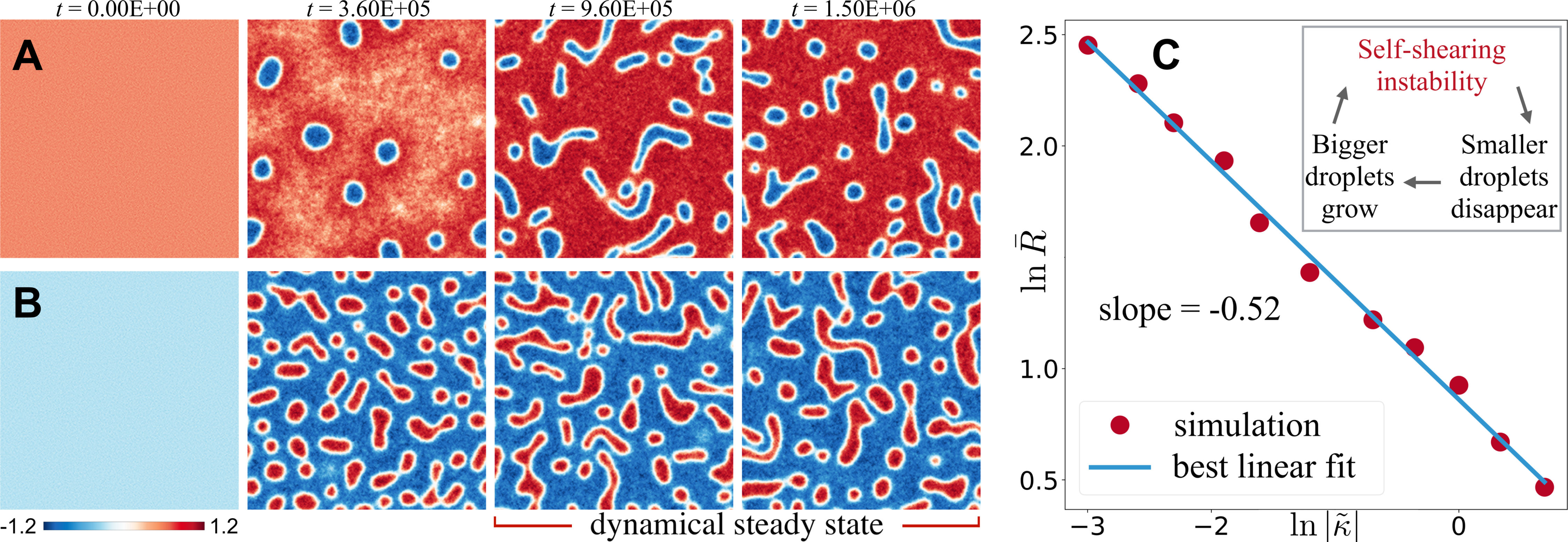
Figure 1: The self-shearing instability interrupts phase ordering in two dimensions with contractile active stress. Time sequence A has global density $\phi_{0}=-0.6$ (giving bubbles), while sequence B has $\phi_{0}=0.4$ giving droplets. (Sequences for $\phi_{0}=+0.6,-0.4$ can be generated by inverting the color scale.) Both sequences have $\tilde{\kappa}=-0.1$. Panel C shows the mean steady state droplet size $\bar{R}$ (defined as $(A_{d}/4\pi)^{1/2}$ with $A_{d}$ the droplet area) on variation of $\tilde{\kappa}$. The best linear fit on log-log gives exponent $-0.52$, in good agreement with the scaling argument of (5). System size $256^{2}$; for movies and simulation details see siF .

Active scalar field theory: Our starting point is the diffusive dynamics of a conserved scalar field $\phi(\boldsymbol{r},t)$ in a momentum-conserving fluid of velocity $\boldsymbol{v}(\boldsymbol{r},t)$:

$$\dot{\phi} +\boldsymbol{\nabla}\cdot\boldsymbol{J}+\boldsymbol{v}\cdot\boldsymbol{\nabla}\phi=0.$$ (1)

Here $\boldsymbol{J}$ is the current density of $\phi$, which contains equilibrium, active and stochastic contributions. Keeping active terms to order $\mathcal{O}(\phi^{2},\nabla^{3})$ in (1), $\boldsymbol{J}$ obeys Wittkowski et al. (2014); Tiribocchi et al. (2015); Tjhung et al. (2018)

$$\boldsymbol{J} =M\left(-\boldsymbol{\nabla}\mu+\zeta(\nabla^{2}\phi)\boldsymbol{\nabla}\phi\right)+\sqrt{2DM}\boldsymbol{\Lambda},$$ (2a)

$$\mu =\mu^{E}+\mu^{\lambda},\quad\mu^{E}=\frac{\delta\mathcal{F}}{\delta\phi},\quad\mu^{\lambda}=\lambda|\boldsymbol{\nabla}\phi|^{2}.$$ (2b)

Here $M$ is a mobility, assumed constant (we set $M=1$ in what follows); $\boldsymbol{\Lambda}$ is a zero-mean, unit-variance Gaussian white noise, and $D$ is a noise temperature phi . The equilibrium and non-equilibrium parts of the chemical potential for $\phi$ are denoted by $\mu^{E}$ and $\mu^{\lambda}$, while $\mathcal{F}$ is the Landau-Ginzburg free energy functional: $\mathcal{F}[\phi]=\int\left(\frac{a}{2}\phi^{2}+\frac{b}{4}\phi^{4}+\frac{\kappa}{2}(\boldsymbol{\nabla}\phi)^{2}\right)d\boldsymbol{r}$, which gives bulk phase separation for $a<0$, with $b,\kappa>0$ for stability Bray (1994); Chaikin and Lubensky (2000).

The terms in $\zeta$ and $\lambda$ in (2) break time-reversal symmetry at $\mathcal{O}(\phi^{2},\nabla^{4})$ in (1). These terms also break the $\phi\rightarrow-\phi$ symmetry of the passive limit; however the full system of equations remains invariant under $(\phi,\lambda,\zeta)\rightarrow-(\phi,\lambda,\zeta)$. This means that all statements made below about droplets also apply to the phase-inverted case of bubbles, so long as $\lambda$ and $\zeta$ are also changed in sign. Notably, the reverse Ostwald process stabilizes only droplets for $\zeta<0$ and only bubbles for $\zeta>0$ Tjhung et al. (2018).

The fluid flow, in the limit of low Reynolds number (as applicable to microswimmers), is obtained from the solution of the Stokes equation: $\boldsymbol{\nabla}\cdot\boldsymbol{\sigma}=-\boldsymbol{f},$ where $\boldsymbol{f}=\boldsymbol{\nabla}\cdot(\boldsymbol{\Sigma}^{A}+\boldsymbol{\Sigma}^{E})$ is the force density on the fluid, $\bm{\sigma}=-p\boldsymbol{I}+\eta(\bm{\nabla}\boldsymbol{v}+(\bm{\nabla}\boldsymbol{v})^{T})$ is the Cauchy fluid stress, $\eta$ is viscosity, $\boldsymbol{I}$ is the identity tensor, and $p$ is the pressure field which contains all isotropic terms and ensures incompressibility ($\nabla\cdot\boldsymbol{v}=0$) Landau and Lifshitz (1959). We neglect noise in these flow equations since this would involve the thermal temperature $T$ which is vastly smaller than $D$ for active swimmers.

There exists a standard procedure Kendon et al. (2001) to derive the deviatoric stress $\boldsymbol{\Sigma}^{E}$ in equilibrium systems using the free energy $\mathcal{F}$. This stress, retaining all isotropic terms, satisfies $\boldsymbol{\nabla}\cdot\boldsymbol{\Sigma}^{E}=-\phi\nabla\mu^{E}$, which is the thermodynamic force density on the fluid due to gradients of the concentration field $\phi$ Bray (1994). The deviatoric stresses $\boldsymbol{\Sigma}^{E}$ and $\boldsymbol{\Sigma}^{A}$ are then, in $d$-dimensions, given to the required order as

$$\boldsymbol{\Sigma}^{E}=-\kappa\boldsymbol{S},\qquad\boldsymbol{\Sigma}^{A}=-(\tilde{\kappa}-\kappa)\boldsymbol{S},$$ (3)

where $\boldsymbol{S}\equiv(\boldsymbol{\nabla}\phi)(\boldsymbol{\nabla}\phi)-\tfrac{1}{d}|\boldsymbol{\nabla}\phi|^{2}\boldsymbol{I}$. The mechanical stress $\boldsymbol{\Sigma}^{A}+\boldsymbol{\Sigma}^{E}=-\tilde{\kappa}\boldsymbol{S}$ is not derived from a free energy and breaks detailed balance in general. Its overall coefficient $\tilde{\kappa}$ can be either positive (for extensile microswimmers) or negative (for sufficiently contractile ones) Tiribocchi et al. (2015), unlike equilibrium systems where $\boldsymbol{\Sigma}^{A}=0$.

Equations (1-3) define our Active Model H for the diffusive dynamics of a conserved order parameter with momentum conservation.The numerical method we use to integrate these equations is described in siF . Having neglected inertia, they reduce to an effective dynamics for $\phi$ alone, which reads (with $M=1$)

$$\dot{\phi}=\nabla^{2}\mu^{\text{eff}}-\boldsymbol{\nabla}\phi(\boldsymbol{r})\cdot\int\mathbf{G}(\boldsymbol{r}-\boldsymbol{r}^{\prime})\cdot\boldsymbol{f}(\boldsymbol{r}^{\prime})\,d\boldsymbol{r}^{\prime}-\boldsymbol{\nabla}\cdot\boldsymbol{J}^{\Lambda}.$$ (4)

Here $\mathbf{G}(\boldsymbol{r})$ is the Oseen tensor, $\boldsymbol{J}^{\Lambda}=\sqrt{2D}\boldsymbol{\Lambda}$, and $\mu^{\text{eff}}=\mu^{E}+\mu^{\lambda}+\mu^{\zeta}$ an effective chemical potential. This has a part $\mu^{\zeta}$, constructed via Helmholtz decomposition of the active current term in (2), as $\zeta(\nabla^{2}\phi)\boldsymbol{\nabla}\phi=-\boldsymbol{\nabla}\mu^{\zeta}+\boldsymbol{\nabla}\times\boldsymbol{A}$. The $\boldsymbol{\nabla}\times\boldsymbol{A}$ term is divergenceless, and so cannot contribute to $\dot{\phi}$ in (4), allowing it to be ignored Tjhung et al. (2018).

Three tensions: At large scales, the dynamics of an interface between phases is controlled by its curvature and its interfacial tension. Without activity, there is only one such tension, $\gamma_{{0}}$$=\sqrt{-8\kappa a^{3}/9b^{2}}$, governing both diffusive and mechanical sectors; curvature then drives diffusive currents and/or fluid flow via Laplace pressure Bray (1994); Cates and Tjhung (2018).

With activity, two further tensions enter Tjhung et al. (2018); Tiribocchi et al. (2015). First, the chemical potential term $\mu^{\zeta}$ is in general nonlocal, and acquires a step-discontinuity across a curved interface that is cancelled by a counter-step in $\mu^{E}$. The result is a discontinuity in $\phi$ different from the equilibrium one. This is captured by a ‘pseudotension’ $\gamma_{\phi}$ that replaces $\gamma_{{0}}$ when calculating diffusive fluxes between droplets, and becomes negative for sufficiently negative $\zeta,\lambda$. Crucially, negative $\gamma_{\phi}$ does not make interfaces locally unstable; spherical droplets stay spherical. Rather, its effect is to drive the system towards states of globally uniform curvature (monodisperse drops) whereas positive tension promotes curvature differences by shrinking small droplets and growing large ones (the Ostwald process) Tjhung et al. (2018).

The third tension arises from the active stress at interfaces, where swimmers align parallel or antiparallel to the surface normal. In either case, contractile swimmers pull fluid inward along the normal direction and expel it in the interfacial plane, causing stretching, whereas extensile swimmers do the opposite. The resulting mechanical tension is $\gamma_{v}=\tilde{\kappa}\gamma_{{0}}/{\kappa}$, which is negative for sufficient contractility; this is known to interrupt phase separation for bicontinuous regimes Tiribocchi et al. (2015). We find next that it also does so for droplets, by destabilizing interfaces locally (in contrast with negative $\gamma_{\phi}$; see above).

Self-shearing instability: For simplicity we first consider active mechanical stress alone, setting $\lambda=\zeta=0$ so that $\gamma_{\phi}=\gamma_{{0}}>0$ while $\tilde{\kappa}=-0.1$, giving negative $\gamma_{v}$. In Fig.(1), we show the dynamic interruption of phase separation in two dimensions and the resulting steady state droplet size $\bar{R}$. The negative mechanical tension, arising from contractile stress, results in a self-shearing of the droplets, causing large ones to split. This is balanced by Ostwald ripening: small droplets evaporate while large ones grow until they in turn become unstable. The result is a dynamical steady state of droplet splitting followed, on average, by diffusive growth of one offspring and disappearance of the other(s). Supplemental movies show this dynamics clearly siF . In Fig.(2), and supplemental movie siF , we show the dynamics of an individual droplet for negative $\gamma_{v}$, which exhibits the flow-induced droplet breakup mechanism. Our numerics do not of course directly introduce a negative interfacial tension, but solve the full equations (1-3) or equivalently (4).

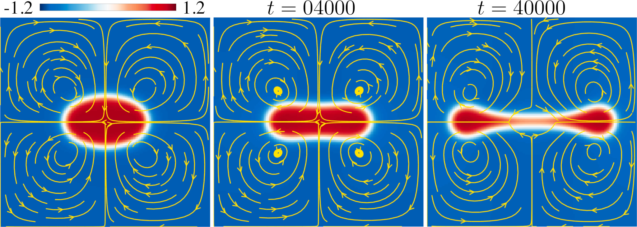
Figure 2: Snapshots mapping the order parameter and flow streamlines, starting from a deformed droplet for a sufficiently contractile active stress (self-shearing instability).

Scaling of droplet size: In Fig.1C, we show that the droplet size obeys $\bar{R}\sim|\gamma_{v}/\gamma_{{\phi}}|^{-0.52}$ (best fit exponent), where, in these simulations, $\gamma_{\phi}=\gamma_{{0}}>0$. We now argue on simple grounds for a negative one half exponent whenever $\gamma_{v}<0$ and $\gamma_{\phi}>0$. From the mechanical tension $\gamma_{v}$ and fluid parameters we can construct just one quantity with the dimensions of velocity: ${\cal V}_{v}=\gamma_{v}/\eta$. This is the familiar coarsening rate $\dot{L}$ for systems with bicontinuous domains of size $L$, in the so-called ‘viscous hydrodynamic’ regime where curvature drives fluid motion and diffusive fluxes are negligible Kendon et al. (2001). For a droplet of size $\bar{R}$ with negative $\gamma_{v}$, one thus expects the time between scission events to scale as $\tau=-\bar{R}/{\cal V}_{v}$. The Ostwald process gives another speed, which is the rate of change of the mean droplet size ${\cal V}_{\phi}(\bar{R})=\dot{\bar{R}}\propto{M\gamma_{\phi}}/{\phi_{B}^{2}\bar{R}^{2}}$ where $\phi_{B}$ is the binodal density Bray (1994); Tjhung et al. (2018). Balancing a positive Ostwald speed ${\cal V}_{\phi}(\bar{R})$ with a negative hydrodynamic speed ${\cal V}_{v}$ gives the promised scaling law

$$\bar{R}\propto\left(\frac{-\gamma_{v}\phi_{B}^{2}}{\eta M\gamma_{\phi}}\right)^{-1/2}\sim\left|\frac{\gamma_{v}}{\gamma_{\phi}}\right|^{-1/2}\,.$$ (5)

The predicted one-half exponent is in excellent agreement with Fig.1C. Unlike the simulations, our scaling argument does not include noise, which appears inessential to the steady state, at least in the parameter range investigated here. We checked this by explicitly switching off noise once the steady state is achieved and found that it continues to exist, with essentially the same droplet life-cycle and mean size. While noise is needed initially to start the phase separation, once enough droplets are present the contractile active stress can maintain the dynamics of scission and coarsening indefinitely. In addition to splitting and ripening, we observe splitting-induced coalescence mediated by fluid flow. This resembles the coalescence-induced coalescence mechanism seen for semidilute passive droplets in two dimensions Wagner and Cates (2001). However, this cannot change the scaling because its physics is also governed by ${\cal V}_{\phi}$.

Competing activity channels: We next consider the full dynamics of (4), where both the active tensions can change sign, and enumerate the possible steady-states. The resulting phase diagram, in the $(\gamma_{\phi},\gamma_{v})$ plane, is shown in Fig.(3A-B). In panel A, we show time evolution of two bubbles of unequal sizes and their final steady state. The two bubbles disproportionate if both tensions are positive; the corresponding outcome in the many-droplet system (panel B) is forward Ostwald dynamics. The three activity parameters $\tilde{\kappa},\lambda,\zeta$ in this region serve merely to renormalize the passive behavior. In contrast, when $\gamma_{v}>0$ and $\gamma_{\phi}<0$, we recover the result of Tjhung et al. (2018), with reverse Ostwald ripening arresting phase separation of droplets (see panel C(ii)). As in the forward case, the reverse Ostwald regime entails little or no fluid motion, so the results given in Tjhung et al. (2018) apply even for the wet systems studied here, with physics controlled by $\gamma_{\phi}$ and no role for $\gamma_{v}$. Thirdly, the case $\gamma_{v}<0$ and $\gamma_{\phi}>0$ is governed by our interrupted steady state with the splitting/coarsening life-cycle described above; here $\lambda$ and $\zeta$ enter only via $\gamma_{\phi}$. Because the steady state balances mechanical and diffusive processes, both tensions enter the mean droplet size via (5).

In the final regime, both tensions are negative. Here, because negative $\gamma_{\phi}$ reverses Ostwald ripening, the balance of splitting and ripening embodied in (5) cannot be maintained. Were splitting to continue, the number of droplets would increase forever, with the reverse Ostwald process driving these towards uniformity in size but not allowing the number to reduce by evaporation. Accordingly, for negative $\gamma_{\phi}$, no matter how small its magnitude, the steady state must consist of almost static droplets with no splitting, and this is indeed what we observe.

Despite this complete change of mechanism, we now argue that the steady-state droplet size is still governed by $\bar{R}\sim|\gamma_{v}|^{-1/2}$ as in (5). This is because the reverse Ostwald process drives the system towards uniformity of curvature which, for a single droplet, directly opposes the self-shearing instability. Indeed, for an amplitude ${\cal A}\sim\epsilon R$ of the lowest deformation mode in a droplet of radius $R$, one expects on dimensional grounds that, up to prefactors, $\dot{{\cal A}}\sim\epsilon({\cal V}_{v}+{\cal V}_{\phi}(R))$. Here the first term is the self-shearing instability and the second is stabilizing for negative $\gamma_{\phi}$. Stability is restored for droplets smaller than $\bar{R}$ given by (5), which thus again gives the scaling of steady-state droplet size, albeit by a completely different mechanism of arrest rather than interruption. This scaling is consistent with simulations, see Fig.(3D).

All the above arguments apply equally to bubbles as to droplets via invariance under $(\phi,\lambda,\zeta)\to-(\phi,\lambda,\zeta)$.

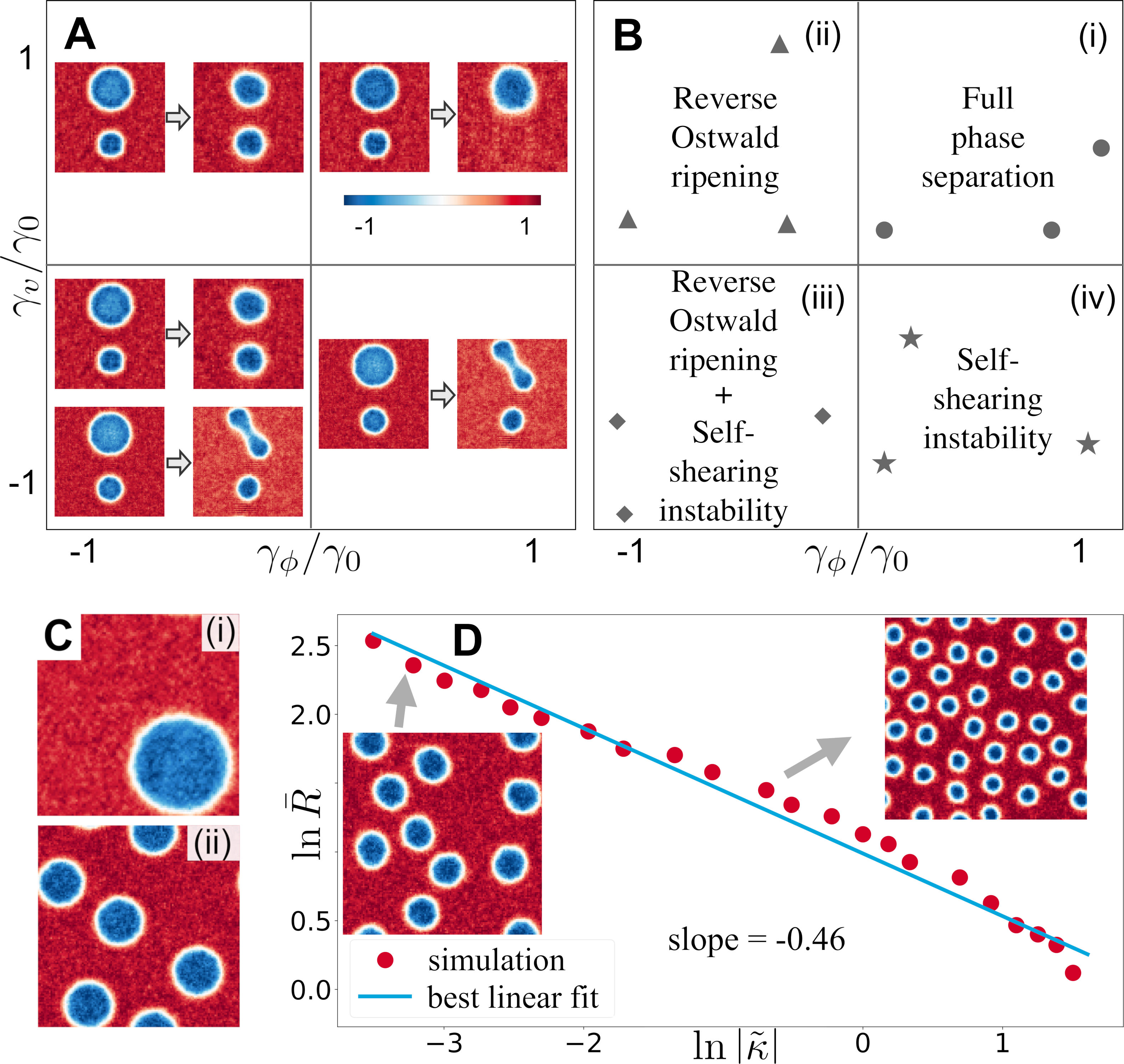
Figure 3: Phases of Active Model H in the plane $(\gamma_{\phi},\gamma_{v})$. Panel A shows the dynamics of two unequal size bubbles in four regions distinguished by the signs of $\gamma_{\phi}$ and $\gamma_{v}$, as labelled in B. The markers denote simulation points. Snapshots of steady states are shown in panel C(i-ii) for the regions in panel B(i-ii). Panel D shows that $\bar{R}\sim|\gamma_{v}|^{-1/2}$ (5) continues to hold (best fit exponent is $-0.46$) in the region B(iii). See Fig(1) for steady states of B(iv). System size is $128^{2}$.

Conclusion: In wet active systems containing droplets or bubbles, microphase separation can replace bulk phase separation by three distinct mechanisms. These are reverse Ostwald ripening (also present in the dry limit, and caused by negative pseudotension $\gamma_{\phi}$); hydrodynamic interruption by self-shearing (caused by negative mechanical tension $\gamma_{v}$); and a peculiar combination of the two when both of tensions are negative. In contrast to reverse Ostwald ripening, where the size of droplets or bubbles in the arrested steady state is selected by noise (or, in its absence, initial conditions) Tjhung et al. (2018), our self-shearing mechanism continues to operate even if the noise is switched off after the steady-state is reached. The droplet size is then selected by a balance between droplet splitting and forward Ostwald ripening. This balance is unsustainable when $\gamma_{\phi}$ is also negative, and so is replaced by a new one whereby the reverse Ostwald process suppresses the self-shearing instability for small droplets, leading to static arrest rather than dynamic interruption.

These results point to a subtle interplay of causes behind the phenomena of active microphase separation. We contend that they cannot be understood without first clearly enumerating the relevant activity channels, and then studying their interaction; this is best done within the minimalist framework of an active field theory as done here. A possible generalization of (4) would allow for boundary conditions imposed on the fluid flow via a nearby wall; these are known to play a crucial role in active phase separation Singh and Adhikari (2016); Thutupalli et al. (2018); Singh et al. (2019) but with no clear understanding, so far, of the microphase-separated case.

Our findings should complement more detailed work that could connect our activity channels to microscopic interactions Liebchen et al. (2015, 2017); Alarcón et al. (2017); Saha et al. (2014); Agudo-Canalejo and Golestanian (2019). They may also be be relevant to continuum models of multiple species (some non-conserved Zwicker et al. (2017)) that were used recently to study microphase separations used by cells to create cytoplasmic and nucleoplasmic organization Shin and Brangwynne (2017); Weber et al. (2019). Fluid motion is often neglected in such studies but we have shown that it brings new features (a similar case of elasticity in polymer networks has been shown to arrest phase separation Style et al. (2018)), suggesting exciting directions for future work.

Acknowledgements: We thank Ronojoy Adhikari and Elsen Tjhung for useful discussions. RS is funded by a Royal Society-SERB Newton International Fellowship. MEC is funded by the Royal Society. Numerical work was performed on the Fawcett HPC system at the Centre for Mathematical Sciences. Work funded in part by the European Research Council under the Horizon 2020 Programme, ERC grant agreement number 740269.

Supplemental information (SI)

Appendix A Methodology

In this section, we explain the numerical methods used to study the field theory of an active scalar field with mass and momentum conservation. We first explain the solution of the flow equations and then given details of the simulation and provide the system of parameters.

Figure	Global density $\phi_{0}$	System size	$\tilde{\kappa}$	$\lambda$	$\zeta$
1 A	0.6	$256\times 256$	-0.1	0	0
1 B	-0.4	$256\times 256$	-0.1	0	0
1 C	0.6	$128\times 128$	varied	0	0
2	-0.1	$128\times 128$	-0.1	0	0
3 A	0.6	$128\times 128$	varied	varied	varied
3 B	0.6	$128\times 128$	varied	varied	varied
3 C(i)	0.6	$128\times 128$	1.1	0	0
3 C(ii)	0.6	$128\times 128$	1.1	1.2	2
3 D	0.6	$128\times 128$	varied	1.2	2

Table 1: Simulation parameters used to study the field theory of an active scalar with mass and momentum conservation. Throughout the paper, the following parameters have been kept fixed $a=-0.25$, $b=0.25$, $\kappa=1$, $M=1$, and $D=0.02$. The value of $\tilde{\kappa}$ has been varied in Fig.(1C) and Fig.(3D) to show the scaling of the length scale with contractile activity. We start with an elliptic droplet in 2A and 2B. The parameters for activity in mass conservation ($\lambda$, $\zeta$) and momentum conservation ($\tilde{\kappa}$) equations has been varied in Fig.(3A-B) to enumerate distinct steady states. All the simulations reported are in two space dimensions, while the predictions of the manuscript would be maintained in higher dimensions.

A.1 Stokes solver

At low Reynolds number, the fluid flow satisfies the Stokes equation

$$-\boldsymbol{\nabla}p+\eta\nabla^{2}\boldsymbol{v} =-\boldsymbol{f},$$ (6)

$$\boldsymbol{\nabla}\cdot\boldsymbol{v} =0.$$ (7)

Here,

$$\boldsymbol{f}=\boldsymbol{\nabla}\cdot(\boldsymbol{\Sigma}^{A}+\boldsymbol{\Sigma}^{E}),$$

is the force density on the fluid. We now show how to determine flow given the force density and detail the implementation of incompressibility in the flow. We use Fourier transforms to obtain a solution of the above equations. We define the Fourier transform of a function $\varphi(\boldsymbol{r})$ as

$$\hat{\varphi}(\boldsymbol{k})=\mathbb{\mathbb{F}}\left[\varphi(\boldsymbol{r})\right]=\int\varphi(\boldsymbol{r})\,e^{-i\boldsymbol{k}\cdot\boldsymbol{r}}\,d\boldsymbol{r},$$ (8a)

$$\varphi(\boldsymbol{r})=\mathbb{\mathbb{F}}^{-1}\left[\hat{\varphi}(\boldsymbol{k})\right]=\frac{1}{(2\pi)^{3}}\int\hat{\varphi}(\boldsymbol{k})\,e^{i\boldsymbol{k}\cdot\boldsymbol{r}}\,d\boldsymbol{k}.$$ (8b)

We now Fourier transform (6) to obtain

$$-i\boldsymbol{k}\hat{p}-\eta k^{2}\boldsymbol{\hat{v}} =-\boldsymbol{\hat{f}},$$ (9a)

$$i\boldsymbol{k}\cdot\boldsymbol{\hat{v}} =0.$$ (9b)

The above equations can then be used to obtain the Fourier transform of the pressure field

$$\hat{p}=-i\boldsymbol{k}\cdot\boldsymbol{\hat{f}}/k^{2}.$$ (10)

The above expression of the pressure is then used in (9a) to obtain the solution of the fluid flow, with built-in incompressibility, given as

$$\boldsymbol{\hat{v}} =\mathbf{\hat{G}}(\boldsymbol{k})\cdot\boldsymbol{\hat{f}},\quad\quad\mathbf{\hat{G}}(\boldsymbol{k})=\frac{1}{\eta}\left(\frac{\boldsymbol{I}}{k^{2}}-\frac{\boldsymbol{k}\boldsymbol{k}}{k^{4}}\right).$$ (11)

Here $\mathbf{\hat{G}}(\boldsymbol{k})$ is the Fourier transform of the Oseen tensor $\mathbf{G}(\boldsymbol{r})$ Pozrikidis (1992). The explicit forms of the Oseen tensor, in three dimensions, is

$$\mathbf{G}(\boldsymbol{r}) =\frac{1}{8\pi\eta}\left(\frac{\boldsymbol{I}}{r}+\frac{\boldsymbol{r}\boldsymbol{r}}{r^{3}}\right).$$ (12)

The above is the Green’s function of Stokes equation in an unbounded domain and captures the long range interactions at low Reynolds number Happel and Brenner (1965). It should be noted that we are confining ourselves to low Reynolds number by not solving the full Navier-Stokes equation. Thus, our theory is mainly applicable to active matter systems of microorganisms Lauga and Powers (2009) and synthetic microwswimmers Ebbens and Howse (2010), where the Reynolds number is known to be very small.

A.2 Simulation details

The simulations reported in this manuscript are performed by the numerical integration of Eq.(1-3) of the main text. Eq.(11) is the solution for the fluid flow, which we use for numerical computations. The solution, by construction, satisfies incompressibility exactly. The Fourier solution of the fluid flow is then used in Eq.(1) to numerical update the order parameter field. The terms in the mass conservations equations are computed using a pseudospectral method (involving Fourier transforms and 2/3 dealiasing procedure) Orszag (1971); Boyd (2000). The spectral solver for the fluid flow and order parameter is numerically implemented using standard fast Fourier transforms (FFTs) and by virtue of these Fourier transforms, periodic boundary conditions are automatically ensured in the system. We evolve the system in time using the explicit Euler–Maruyama method Kloeden and Platen (1992). We provide the parameters used in generating all the figures of the manuscript in Table 1.

Appendix B Higher-order terms of active stress

In the main text, we have provided a form of the active stress tensor $\boldsymbol{\Sigma}^{A}$ in Eq.(3). This term preserves the $\phi\rightarrow-\phi$ symmetry of the passive model H. It is possible to add higher-order terms of the form $\sim-\left(\alpha\phi\right)\,\boldsymbol{S}$ and $\sim-\left(\beta\nabla^{2}\phi\right)\,\boldsymbol{S}$ to the active stress tensor. These terms break the $\phi\rightarrow-\phi$ and can be derived by taking into account the fact that self-propulsion speed of active particles is dependent on their local density Tailleur and Cates (2008); Cates and Tailleur (2015); Tiribocchi et al. (2015). In what follows, we show that such terms can never reverse the sign of the active stress. In other words, it is not possible to make a contractile swimmer by slowing down an extensile swimmer.

To obtain terms of the form $\sim-\left(\alpha\phi\right)\,\boldsymbol{S}$ and $\sim-\left(\beta\nabla^{2}\phi\right)\,\boldsymbol{S}$, we note that the density-dependent speed $w([\phi])$ of active particles can be written as $w([\phi])=w_{0}+w_{1}\phi+w_{2}\nabla^{2}\phi+\text{higher order terms}$ Tailleur and Cates (2008). The active stress can be written as $\boldsymbol{\Sigma}^{A}\sim\xi_{P}p_{i}p_{j}$, where $p_{i}=-\tau\nabla_{i}(w\phi)$ and $\tau$ is the orientational relaxation time Tiribocchi et al. (2015). Thus, it follows that the active stress is $\Sigma_{ij}^{A}=\Upsilon S_{ij}$, with $\Upsilon\sim\xi_{P}\tau^{2}(w_{0}+2w_{1}\phi+w_{2}\nabla^{2}\phi+\text{h.o.t})^{2}$. It is then clear that the sign of the coefficients in the active stress is determined by the parameter $\xi_{P}$, which is positive for extensile swimmer and negative for contractile swimmers. For simplicity, we have treated $\xi_{P}$ as constant but making it a function of $w$ has no effect on our conclusions in the paper. Moreover, by construction, the terms proportional to $\alpha$ and $\beta$ can only reduce the magnitude but never reverse the sign of the active stress. Thus, in this paper, we consider a constant $\Upsilon$ which captures all the qualitative effects.

Appendix C Supplemental movies

In this Appendix, we describe the supplemental movies which are complementary with the main text. These movies are available online at at this URL.

Movie I: The movie shows the dynamics of Fig.1A in the main text, which is the self-shearing instability in the bubble phase for contractile active stress ($\tilde{\kappa}<0$) with no activity in the diffusive sector. Starting from a uniform phase, droplets nucleate due to the noise and they grow in size until interrupted by the contractile active stress. The parameters are $a=-0.25$, $b=0.25$, $\kappa=1$, $\tilde{\kappa}=-0.1$, $\lambda=0$, and $\zeta=0$. The initial global density $\phi_{0}=0.6$ and the system size is $256\times 256$.

Movie II: Same as in movie I but with $\phi_{0}=-0.4$. It corresponds to Fig.(1B) of the main text.

Movie III: The movie shows the fluid flow and dynamics of deformed droplet in the presence of a sufficiently contractile active stress (self-shearing instability). It corresponds to Fig(2) of the main text. The parameters are $a=-0.25$, $b=0.25$, $\kappa=1$, $\lambda=0$, $\zeta=0$, and $\tilde{\kappa}=-0.1$. The system size used for this simulation is $256\times 256$.

Movie IV: Nucleation and growth of bubbles when activity is present in both the mechanical and diffusive sectors. A snapshot from the steady state is in Fig(3C-(ii)) of the main text. The parameters are $a=-0.25$, $b=0.25$, $\kappa=1$, $\tilde{\kappa}=1.1$, $\lambda=1$, $\zeta=2$. The initial global density $\phi_{0}=0.6$ and the system size is $128\times 128$.

Movie V: Same as in movie IV, but with $\tilde{\kappa}=-0.1$. It corresponds to Fig.(3D) in the main text. The fluid due to contractile stress has the effect of stretching the interface, which is the precursor to the self-shearing instability as the system approaches the steady state. It should be noted that there is no self-shearing in the steady state - this is because the reverse Ostwald process drives the system towards uniformity of curvature which directly opposes the self-shearing instability.

References

- Ebbens and Howse (2010) S. J. Ebbens and J. R. Howse, “In pursuit of propulsion at the nanoscale,” Soft Matter 6, 726–738 (2010).
- Palacci et al. (2013) J. Palacci, S. Sacanna, A. P. Steinberg, D. J. Pine, and P. M. Chaikin, “Living crystals of light-activated colloidal surfers,” Science 339, 936–940 (2013).
- Theurkauff et al. (2012) I. Theurkauff, C. Cottin-Bizonne, J. Palacci, C. Ybert, and L. Bocquet, “Dynamic clustering in active colloidal suspensions with chemical signaling,” Phys. Rev. Lett. 108, 268303 (2012).
- Buttinoni et al. (2013) I. Buttinoni, J. Bialké, F. Kümmel, H. Löwen, C. Bechinger, and T. Speck, “Dynamical clustering and phase separation in suspensions of self-propelled colloidal particles,” Phys. Rev. Lett. 110, 238301 (2013).
- Ginot et al. (2018) F. Ginot, I. Theurkauff, F. Detcheverry, C. Ybert, and C. Cottin-Bizonne, “Aggregation-fragmentation and individual dynamics of active clusters,” Nat. Comm. 9, 696 (2018).
- Liebchen et al. (2015) B. Liebchen, D. Marenduzzo, I. Pagonabarraga, and M. E. Cates, “Clustering and pattern formation in chemorepulsive active colloids,” Phys. Rev. Lett. 115, 258301 (2015).
- Liebchen et al. (2017) B. Liebchen, D. Marenduzzo, and M. E. Cates, “Phoretic interactions generically induce dynamic clusters and wave patterns in active colloids,” Phys. Rev. Lett. 118, 268001 (2017).
- Alarcón et al. (2017) F. Alarcón, C. Valeriani, and I. Pagonabarraga, “Morphology of clusters of attractive dry and wet self-propelled spherical particle suspensions,” Soft matter 13, 814–826 (2017).
- Saha et al. (2014) S. Saha, R. Golestanian, and S. Ramaswamy, “Clusters, asters, and collective oscillations in chemotactic colloids,” Phys. Rev. E 89, 062316 (2014).
- Agudo-Canalejo and Golestanian (2019) J. Agudo-Canalejo and R. Golestanian, “Active phase separation in mixtures of chemically interacting particles,” Phys. Rev. Lett. 123, 018101 (2019).
- Stenhammar et al. (2016) J. Stenhammar, R. Wittkowski, D. Marenduzzo, and M. E. Cates, “Light-induced self-assembly of active rectification devices,” Sci. Adv. 2, e1501850 (2016).
- Hohenberg and Halperin (1977) P. C. Hohenberg and B. I. Halperin, “Theory of dynamic critical phenomena,” Rev. Mod. Phys. 49, 435 (1977).
- Tailleur and Cates (2008) J. Tailleur and M. E. Cates, “Statistical mechanics of interacting run-and-tumble bacteria,” Phys. Rev. Lett. 100, 218103 (2008).
- Cates and Tailleur (2015) M. E. Cates and J. Tailleur, “Motility-induced phase separation,” Annu. Rev. Condens. Mat. Phys. 6, 219–244 (2015).
- Marchetti et al. (2013) M. C. Marchetti, J. F. Joanny, S. Ramaswamy, T. B. Liverpool, J. Prost, Madan Rao, and R. A. Simha, “Hydrodynamics of soft active matter,” Rev. Mod. Phys. 85, 1143–1189 (2013).
- Cates and Tjhung (2018) M. E. Cates and E. Tjhung, “Theories of binary fluid mixtures: from phase-separation kinetics to active emulsions,” J. Fluid Mech. 836, P1 (2018).
- Wittkowski et al. (2014) R. Wittkowski, A. Tiribocchi, J. Stenhammar, R. J. Allen, D. Marenduzzo, and M. E. Cates, “Scalar field theory for active-particle phase separation,” Nat. Comm. 5, 4351 (2014).
- Tjhung et al. (2018) E. Tjhung, C. Nardini, and M. E. Cates, “Cluster phases and bubbly phase separation in active fluids: Reversal of the ostwald process,” Phys. Rev. X 8, 031080 (2018).
- Bray (1994) A. J. Bray, “Theory of phase-ordering kinetics,” Adv. Phys. 43, 357 (1994).
- Tiribocchi et al. (2015) A. Tiribocchi, R. Wittkowski, D. Marenduzzo, and M. E. Cates, “Active model H: scalar active matter in a momentum-conserving fluid,” Phys. Rev. Lett. 115, 188302 (2015).
- (21) “See supplemental material in the appendix, which includes the detailed calculations, numerical method, and descriptions of the supplemental movies.” .
- (22) “Giving different dependences to and would introduce a further channel for time-reversal symmetry breaking, but this is not motivated by microscopic models of active particles Stenhammar et al. (2013),” .
- Chaikin and Lubensky (2000) P. M. Chaikin and T. C. Lubensky, Principles of condensed matter physics (Cambridge University Press, 2000).
- Landau and Lifshitz (1959) L. D. Landau and E. M. Lifshitz, Fluid mechanics (Pergamon Press, New York, 1959).
- Kendon et al. (2001) V. M. Kendon, M. E. Cates, I. Pagonabarraga, J-C Desplat, and P. Bladon, “Inertial effects in three-dimensional spinodal decomposition of a symmetric binary fluid mixture: a lattice Boltzmann study,” J. Fluid Mech. 440, 147–203 (2001).
- Wagner and Cates (2001) A. J. Wagner and M. E. Cates, “Phase ordering of two-dimensional symmetric binary fluids: A droplet scaling state,” Europhys. Lett. 56, 556 (2001).
- Singh and Adhikari (2016) R. Singh and R. Adhikari, “Universal hydrodynamic mechanisms for crystallization in active colloidal suspensions,” Phys. Rev. Lett. 117, 228002 (2016).
- Thutupalli et al. (2018) S. Thutupalli, D. Geyer, R. Singh, R. Adhikari, and H. A. Stone, “Flow-induced phase separation of active particles is controlled by boundary conditions,” Proc. Natl. Acad. Sci. 115, 5403–5408 (2018).
- Singh et al. (2019) R. Singh, R. Adhikari, and M. E. Cates, “Competing chemical and hydrodynamic interactions in autophoretic colloidal suspensions,” J. Chem. Phys. 151, 044901 (2019).
- Zwicker et al. (2017) D. Zwicker, R. Seyboldt, C. A Weber, A. A. Hyman, and F. Jülicher, “Growth and division of active droplets provides a model for protocells,” Nat. Phys. 13, 408 (2017).
- Shin and Brangwynne (2017) Y. Shin and C. P. Brangwynne, “Liquid phase condensation in cell physiology and disease,” Science 357, eaaf4382 (2017).
- Weber et al. (2019) C. A. Weber, D. Zwicker, F. Jülicher, and C. F. Lee, “Physics of active emulsions,” Rep. Prog. Phys. 82, 064601 (2019).
- Style et al. (2018) R. W. Style, T. Sai, N. Fanelli, M. Ijavi, K. Smith-Mannschott, Q. Xu, L. A. Wilen, and E. R. Dufresne, “Liquid-liquid phase separation in an elastic network,” Phys. Rev. X 8, 011028 (2018).
- Stenhammar et al. (2013) J. Stenhammar, A. Tiribocchi, R. J. Allen, D. Marenduzzo, and M. E. Cates, “Continuum theory of phase separation kinetics for active brownian particles,” Phys. Rev. Lett. 111, 145702 (2013).
- Pozrikidis (1992) C. Pozrikidis, Boundary Integral and Singularity Methods for Linearized Viscous Flow (Cambridge University Press, 1992).
- Happel and Brenner (1965) J. Happel and H. Brenner, Low Reynolds number hydrodynamics: with special applications to particulate media, Vol. 1 (Prentice-Hall, 1965).
- Lauga and Powers (2009) E. Lauga and T. R. Powers, “The hydrodynamics of swimming microorganisms,” Rep. Prog. Phys. 72, 096601 (2009).
- Orszag (1971) S. A. Orszag, “On the elimination of aliasing in finite-difference schemes by filtering high-wavenumber components,” J. Atmos. Sci. 28, 1074–1074 (1971).
- Boyd (2000) J. P. Boyd, Chebyshev and Fourier spectral methods (Dover, 2000).
- Kloeden and Platen (1992) P. E. Kloeden and E. Platen, Numerical solution of stochastic differential equations (Springer, 1992).