Lattice Boltzmann Electrokinetics simulation of nanocapacitors

Abstract

We propose a method to model metallic surfaces in Lattice Boltzmann Electrokinetics simulations (LBE), a lattice-based algorithm rooted in kinetic theory which captures the coupled solvent and ion dynamics in electrolyte solutions. This is achieved by a simple rule to impose electrostatic boundary conditions, in a consistent way with the location of the hydrodynamic interface for stick boundary conditions. The proposed method also provides the local charge induced on the electrode by the instantaneous distribution of ions under voltage. We validate it in the low voltage regime by comparison with analytical results in two model nanocapacitors: parallel plate and coaxial electrodes. We examine the steady-state ionic concentrations and electric potential profiles (and corresponding capacitance), the time-dependent response of the charge on the electrodes, as well as the steady-state electro-osmotic profiles in the presence of an additional, tangential electric field. The LBE method further provides the time-dependence of these quantities, as illustrated on the electro-osmotic response. While we do not consider this case in the present work, which focuses on the validation of the method, the latter readily applies to large voltages between the electrodes, as well as to time-dependent voltages. This work opens the way to the LBE simulation of more complex systems involving electrodes and metallic surfaces, such as sensing devices based on nanofluidic channels and nanotubes, or porous electrodes.

I Introduction

Interfaces between metals and electrolyte solutions play the central role in electrochemistry as well as in many analytical chemistry techniques. Electrodes are also necessary to apply electric field to manipulate charged objects in solutions, such as colloidal particles or electrolytes. As a result, electrode-electrolyte interfaces have been extensively studied both experimentally and theoretically for well over a century. Recent technological advances have made it possible to design experimental setups in which electrolyte solutions are confined between electrodes separated by very small distances, down to a few tens or hundreds of nm, or within carbon nanotubes which may also exhibit partially metallic behaviorBlase et al. (1994). The ability to build such nanocapacitors opens the way to new analytical strategies based on electrochemistry with a very limited number of redox-active species, using nanofluidic devicesRassaei et al. (2012); Mathwig and Lemay (2013); Lemay et al. (2013) or thin layer cellsSun and Mirkin (2008), and questions our basic understanding of coupled fluid and charge flows, or electrokinetic phenomena, through single nanotubesBocquet and Charlaix (2010); Siria et al. (2013); Secchi et al. (2016); Jubin et al. (2018).

Significant progress has been made in the understanding of the electric double layer (EDL) at charged or metallic interfaces since the pioneering Gouy-Chapman-Stern theoryGouy (1910); Chapman (1913); Stern (1924). In recent years, simulations has become a powerful tool to predict their structure and dynamics without the need to rely on strong simplifying assumptions, which are generally required to obtain analytical theoretical results. For example, Brownian dynamics simulations allowed to investigate the relaxation of the EDL after a charge transfer eventGrün et al. (2004), treating the metallic electrodes as homogeneously charged surfaces and the solvent as a dielectric continuum. At the atomistic level, the introduction of models allowing to perform molecular simulation of electrodes maintained at a constant potential (as in a perfect metal), rather than constant chargeSiepmann and Sprik (1995); Reed, Lanning, and Madden (2007), opened the way to detailed investigations of electrochemical interfaces. These studies showed the importance of taking the polarization of the metal by the electrolyte into accountMerlet et al. (2013a, b); Limmer et al. (2013); Merlet et al. (2014). However, the computational cost of such atomistic simulations restricts their use to small systems (below 10 nm) and relatively concentrated electrolytes (due to the small number of ions in such small volumes).

The dynamics of ions in the bulk and in EDLs, and in turn the charging dynamics of nanocapacitors, results from their thermal motion (diffusion) and their migration due to the local electric field they experience. Taking these factors into account allows to provide a detailed description of the charging dynamics in capacitors in planarBazant, Thornton, and Ajdari (2004); Janssen and Bier (2018) or more complex (e.g. porous) geometriesBiesheuvel and Bazant (2010). Another process by which ions move is their advection by the local fluid flow, which may vanish by symmetry in some simple cases, but cannot be neglected a priori. Together with the fluid flow induced by the net local charge within the EDL, this is at the origin of the above-mentioned electrokinetic phenomena, which have been long studied theoretically or numerically with simulations, from molecularJoly et al. (2004, 2006); Yoshida et al. (2014) to models with various levels of coarse-graining (see e.g. Refs. 26 and 27 for reviews on multiscale simulation approaches).

Among these mesoscopic simulation approaches for electrokinetics (such as Dissipative Particle Dynamics Smiatek et al. (2009) or Multiparticle Collision DynamicsCeratti et al. (2015); Dahirel et al. (2018)), Lattice-BoltzmannSucci (2001) (LB) has emerged as an efficient compromise between the simplicity of the solvent description, based on kinetic theory and allowing to recover proper hydrodynamic behavior, and on the flexibility with which it can be coupled to explicit particles or free energy models to describe complex fluids. In the former case, Molecular Dynamics (MD) coupled to LB was successfully used to investigate the electrokinetic effects with charged colloidsLobaskin, Dünweg, and Holm (2004); Lobaskin et al. (2007), polyelectrolytes in the bulkHickey et al. (2010) or grafted on surfacesHickey and Holm (2013) or their translocation through nanoporesDatar et al. (2017), and more recently (and closer to the subject of the present work) to the response of EDLs to changes in the charge of surfacesLobaskin and Netz (2016).

The other approach, where no explicit particles are present, exists in different flavors, which can broadly be seen as efficient numerical solvers of the continuous electrokinetic equations, even though their roots on kinetic theory also provide additional information on the dynamics of species. In that respect, treating solvent and ions on the same footing in a multi-component LB modelMarini Bettolo Marconi and Melchionna (2012) is a promising approach to capture correlations due in particular to the discrete nature of solvent molecules and ions at this coarse-grained level, especially under extreme confinement (comparable to molecular sizes). For larger systems, the LB method is rather coupled to numerical schemes to describe the evolution of ions. Assuming their instantaneous relaxation (on the time scale over which the fluid evolves) toward the Poisson-Boltzmann equilibrium, for chargedWang, Wang, and Li (2006) or constant-potentialThakore and Hickman (2015) walls, does not allow investigating the relaxation of the ionic concentration and potential profiles in the EDLs. This requires an explicit integration of the ionic dynamics, typically solving the Nernst-Planck equation (described below), via finite differences/elements methods. This has for example been used to simulate electrokinetic effects in porous mediaHlushkou, Kandhai, and Tallarek (2004); Hlushkou et al. (2007) or electrochemical desalinationHlushkou et al. (2016).

An alternative hybrid approach for the dynamics of ions coupled to the LB method for that of the fluid makes a consistent use of the LB lattice. Inspired by previous work based on the moment propagation methodWarren (1997), and extending a previous attempt with ionic fluxes computed on the lattice nodeHorbach and Frenkel (2001), Capuani et al. proposed a method focussing instead on the ionic fluxes through each link connecting nodes of the lattice (via the discrete lattice velocities)Capuani, Pagonabarraga, and Frenkel (2004). This point of view has a number of advantages, such as strictly enforcing charge conservation in particular at solid-liquid boundaries, and offering a statistical interpretation which can be exploited to compute other properties such as velocity auto-correlation functions via moment propagationRotenberg, Pagonabarraga, and Frenkel (2008). This hybrid LB/link-flux method, called Lattice Boltzmann Electrokinetics (LBE), has been successfully used to investigate the dynamics of charged colloidsPagonabarraga, Capuani, and Frenkel (2005); Capuani, Pagonabarraga, and Frenkel (2006); Giupponi and Pagonabarraga (2011); Rempfer et al. (2016); Kuron et al. (2016), charged porous media and ions in oil-water mixturesRotenberg, Frenkel, and Pagonabarraga (2010) or binary colloidal suspensionsRivas et al. (2018). In these systems, electrostatic boundary conditions at solid-liquid interfaces correspond to constant charge (Neumann, i.e. constant normal electric field), rather than constant potential (Dirichlet).

In the present work, we show that a simple rule to impose Dirichlet electrostatic boundary conditions allows the simulation of systems involving metallic surfaces using LBE simulations. Specifically, the method leads to imposing the target potential at the location of the hydrodynamic interface, i.e. between the solid and liquid nodes rather than solely on the solid nodes. In addition, it is possible to determine the instantaneous local charge on the electrode at virtually no additional cost. This opens the way to the simulation of the dynamic response of electric double layers in capacitors by following the evolution of the ionic concentrations and potential profiles as well as the charge of the electrodes. The LBE method naturally also captures the electrokinetic couplings with the solvent. The proposed implementation of electrostatic boundary conditions is readily applicable to arbitrary electrode geometries, just as the bounce-back rule to impose no-slip boundary conditions.

The electrokinetic equations and the LBE algorithm are presented in Section II, together with the proposed method to impose constant-potential boundary conditions and to compute the charge induced on the (blocking) electrode by the instantaneous distribution of ions under voltage. We then demonstrate the validity of the method in Section III by considering capacitors in two geometries, parallel plate and coaxial electrodes, in the regime of small applied voltage, for which analytical results are available (Debye-Hückel theory for the ionic concentration and electric potential profiles, together with Stokes for the steady-state electro-osmotic profiles). We also show numerical results for the transient regime for electro-osmosis in the presence of an additional, tangential electric field, for which no analytical results are available. While we do not consider this case in the present work, which focuses on the validation of the method, the latter readily applies to large voltages between the electrodes.

II Method

II.1 Electrokinetic equations

The canonical description of electrokinetic couplings in a dilute electrolyte consisting of $k$ ionic species with valencies $z_{k}$ and diffusion coefficients $D_{k}$ in a solvent characterized by its mass density $\rho$, dynamic viscosity $\eta$ and dielectric permittivity $\epsilon_{0}\epsilon_{r}$, couples the Poisson-Nernst-Planck equations for the dynamics of ions and the Navier-Stokes equation for that of the solvent. The Nernst-Planck equation is a conservation equation for the ionic concentrations $\rho_{k}$:

$$\frac{\partial\rho_{k}}{\partial t} +\nabla\cdot\left[\rho_{k}{\bf u}+{\bf j}_{k}\right]=$$

$$\frac{\partial\rho_{k}}{\partial t}+\nabla\cdot\left[\rho_{k}{\bf u}-D_{k}\nabla\rho_{k}-\beta D_{k}z_{k}e\rho_{k}\nabla\psi\right]=0$$ (1)

where $\beta=1/k_{B}T$ with $k_{B}$ the Boltzmann constant and $T$ the temperature, $e$ is the elementary charge, ${\bf u}$ is the local velocity of the fluid and where the electrostatic potential $\psi$ satisfies the Poisson equation:

$$\nabla^{2}\psi=-\frac{1}{\epsilon_{0}\epsilon_{r}}\rho_{el}=-\frac{e}{\epsilon_{0}\epsilon_{r}}\sum_{k}\rho_{k}z_{k}\;.$$ (2)

The three terms in the flux defined by Eq. II.1 correspond to advection, diffusion and migration under the effect of the local electric field $-\nabla\psi$, respectively. The advective part depends on the local velocity ${\bf u}$ which is assumed to satisfy the Navier-Stokes equation for an incompressible fluid ($\nabla\cdot{\bf u}=0$):

$$\rho\left(\frac{\partial{\bf u}}{\partial t}+({\bf u}\cdot\nabla){\bf u}\right) =\eta\Delta{\bf u}-\sum_{k}\rho_{k}\nabla\mu_{k}+{\bf f}_{V}^{ext}$$ (3)

with ${\bf f}_{V}^{ext}$ the external force density and the chemical potentials $\mu_{k}=\mu_{k}^{id}+\mu_{k}^{ex}=k_{B}T\ln(\rho_{k}/\rho_{k}^{0})+z_{k}e\psi$ include an ideal part (with $\rho_{k}^{0}$ a reference concentration) and an excess part assumed to arise only from mean-field electrostatic interactions. The excess part results, together with the applied electric field ${\bf E}_{app}$ when present, in a local electric force acting on the fluid $e(\sum_{k}z_{k}\rho_{k})(-\nabla\psi+{\bf E}_{app})$ in Eq. 3.

These coupled equations should be solved for prescribed boundary conditions at solid-liquid interfaces, usually stick (no-slip) for hydrodynamics (${\bf u}=0$) and Neumann (constant field, corresponding to fixed surface charge density) or Dirichlet (constant potential) for electrostatics.

At equilibrium, the ionic fluxes and fluid velocities vanish. From Eq. II.1, the concentration profiles then follow Boltzmann distributions $\rho_{k}=\rho_{k}^{0}e^{-z_{k}\beta e\psi}$. From Eq. 2, the potential satisfies the Poisson-Boltzmann equation:

$$\nabla^{2}\psi =-\frac{e}{\epsilon_{0}\epsilon_{r}}\sum_{k}\rho_{k}^{0}z_{k}e^{-z_{k}\beta e\psi}\;,$$ (4)

which can be linearized for small potentials (Debye-Hückel limit) as:

$$\nabla^{2}\psi =\kappa^{2}\psi=\frac{1}{\lambda_{D}^{2}}\psi\;,$$ (5)

with the Debye screening length:

$$\lambda_{D} =\kappa^{-1}=\left(4\pi l_{B}\sum_{k}\rho_{k}^{0}z_{k}^{2}\right)^{-1/2}\;,$$ (6)

where the Bjerrum length $l_{B}=\frac{\beta e^{2}}{4\pi\epsilon_{0}\epsilon_{r}}$ is the distance at which the Coulomb interaction between two unit charges is equal to the thermal energy ($l_{B}=0.7$ nm in water at room temperature, which corresponds to all the simulation results shown in the rest of this work).

II.2 Lattice Boltzmann Electrokinetics

The Lattice-Boltzmann Electrokinetics (LBE) algorithm is a hybrid lattice scheme coupling the standard Lattice Boltzmann (LB) method for the dynamics of the fluid, which captures in particular overall mass and momentum conservation, with the link-flux method for the evolution of its composition, in particular the diffusion, advection and migration of the ions. Since its introduction by Capuani et al. Capuani, Pagonabarraga, and Frenkel (2004) it has been used and described many times and we only recall the basics to focus on the novelty of the present work, which is the introduction of new electrostatic boundary conditions described in the next section.

The LB method can be derived as a discretized version of a continuous kinetic equation for the evolution of the probability density function $f({\bf r},{\bf v},t)$ to find a fluid particle with a velocity ${\bf v}$ at position ${\bf r}$ at time $t$. The moments of $f$ in velocity space provide the hydrodynamic observables, such as the local density $\rho({\bf r},t)=\int f({\bf r},{\bf v},t){\rm d}{\bf v}$, local mass flux $\rho({\bf r},t){\bf u}({\bf r},t)=\int f({\bf r},{\bf v},t){\bf v}{\rm d}{\bf v}$ and local stress tensor. The Boltzmann equation with the Bhatnagar-Gross-Krook (BGK) collision operator is discretized consistently in space (cubic grid with lattice spacing $\Delta x$), time (with time step $\Delta t$) and velocity space with a finite set of velocities $\{{\bf c}_{i}\}$ with associated populations $f_{i}({\bf r},t)\equiv f({\bf r},{\bf c}_{i},t)$ and weights $w_{i}$. Here we use the three-dimensional D3Q19 lattice Succi (2001), with 19 velocities corresponding to 0, nearest and next-nearest neighbors (with respective norms $0$, $\frac{\Delta x}{\Delta t}$ and $\sqrt{2}\frac{\Delta x}{\Delta t}$ and weights $\frac{1}{3}$, $\frac{1}{18}$ and $\frac{1}{36}$) and a lattice speed unit related to the thermal velocity $c_{s}^{2}=\frac{k_{B}T}{m}=\frac{1}{3}\left(\frac{\Delta x}{\Delta t}\right)^{2}$, with $m$ the mass of the fluid particles.

The local hydrodynamic variables are computed exactly from the populations as:

$$\rho({\bf r},t) =\sum_{i}w_{i}f_{i}({\bf r},t)\;\;;\;\;\rho{\bf u}({\bf r},t)=\sum_{i}w_{i}f_{i}({\bf r},t){\bf c}_{i}$$ (7)

and the populations evolved according to:

$$f_{i}({\bf r}+{\bf c}_{i}\Delta t,t+\Delta t) =f_{i}({\bf r},t)$$

$$\quad-\frac{\Delta t}{\tau}\left[f_{i}({\bf r},t)-f_{i}^{eq}({\bf r},t)\right]+F_{i}({\bf r},t)$$ (8)

where $\tau$ is the characteristic time for the relaxation toward the local Maxwell-Boltzmann distribution $f_{i}^{eq}$ and controls the viscosity of the fluid, while $F_{i}({\bf r},t)$ accounts for the effect of local force density. The latter includes external forces as well as the internal contribution of local chemical potential gradients (see Eq. 3).

The ionic concentrations are discretized on the same spatial grid and time steps and evolved using the link-flux method, separating the contribution of advection from the ones arising from the ideal and excess chemical potential gradients, as described in Ref. 46 to which we refer the reader for the advection part. The contributions of chemical potential gradients are expressed in a symmetrized form by writing the fluxes ${\bf j}_{k}=-D_{k}e^{-\beta\mu_{k}^{ex}}\nabla\left[\rho_{k}e^{+\beta\mu_{k}^{ex}}\right]$. This leads to the update of amount of solutes on each node, $n_{k}({\bf r},t)=\rho_{k}({\bf r},t)\Delta x^{3}$, according to:

$$n_{k}({\bf r},t+\Delta t)-n_{k}({\bf r},t) =-A_{0}\sum_{i}j_{k}^{i}({\bf r},t)$$ (9)

where the sum runs over discrete velocities, $j_{k}^{i}$ is the contribution of each link between ${\bf r}$ and ${\bf r}+{\bf c}_{i}\Delta t$ to the flux of species $k$ through the cell boundary around node ${\bf r}$ and $A_{0}$ is a lattice-dependent geometric factor (equal to $1+2\sqrt{2}$ for D3Q19). The link-fluxes are given by:

$$j_{k}^{i}({\bf r},t) =-d_{k}\frac{e^{-\beta\mu_{k}^{ex}({\bf r})}+e^{-\beta\mu_{k}^{ex}({\bf r}+{\bf c}_{i}\Delta t)}}{2}$$

$$\quad\times\left[\frac{n_{k}({\bf r}+{\bf c}_{i}\Delta t)e^{+\beta\mu_{k}^{ex}({\bf r}+{\bf c}_{i}\Delta t)}-n_{k}({\bf r})e^{+\beta\mu_{k}^{ex}({\bf r})}}{\Delta_{i}}\right]$$ (10)

with $d_{k}=(D_{k}/A_{0})/(\Delta x^{2}/\Delta t)$ and $\Delta_{i}=||{\bf c}_{i}||/(\Delta x/\Delta t)$. While this choice of discretization leads to spurious fluxes when the lattice spacing is too large (large potential differences between neighboring nodes)Rempfer et al. (2016), this form enforces that the ionic concentrations follow the Boltzmann distribution at equilibrium.

At each time step, the excess chemical potentials are computed from the local electrostatic potential determined from the ionic concentrations by solving numerically the Poisson equation as described in the next section. The effect of thermodynamic forces, arising from local excess chemical potential gradients, on the dynamics of the fluid (see Eq. 3) is expressed from the link-fluxes, in dimensionless units, via the term:

$$F_{i}({\bf r},t) =-\frac{c_{s}^{2}}{(\Delta x/\Delta t)^{2}}\sum_{k}\left[\frac{j_{k}^{i}({\bf r},t)}{d_{k}}-\frac{n_{k}({\bf r}+{\bf c}_{i}\Delta t)-n_{k}({\bf r})}{\Delta_{i}}\right]$$ (11)

in Eq. 8.

No-slip hydrodynamic boundary conditions are enforced by the bounce-back rule, which places the interface at the mid-plane between liquid and solid nodes Succi (2001), while setting the link-fluxes to zero through the corresponding links ensures the absence of leakage of ions inside the solid. Together with the advection of ions (see Ref. 46 for more details), the link-flux and LB methods give rise to an evolution of the ionic concentrations and fluid velocity satisfying the coupled Poisson-Nernst-Planck and Navier-Stokes equations II.1, 2 and 3.

II.3 Imposing conducting boundary conditions

The Poisson equation 2 must be solved numerically at each time step to determine the electrostatic potential $\psi({\bf r})$ from the charge distribution $\rho_{el}$ on the lattice. Following previous implementations of the LBE algorithm, we use the Successive Over Relaxation (SOR) method Horbach and Frenkel (2001); Capuani, Pagonabarraga, and Frenkel (2004); Rotenberg, Frenkel, and Pagonabarraga (2010), which we modify as described below to impose constant-potential boundary conditions and to determine the charged induced at the surface of the metal. Introducing the reduced potential $\phi({\bf r})=\beta e\psi({\bf r})$, the Poisson equation can be rewritten as $\nabla^{2}\phi+4\pi l_{B}\frac{\rho_{el}}{e}=0$. Then, we discretize the Laplacian using a stencil consistent with the LB lattice, which can be derived from the Taylor expansion: $\phi({\bf r}+{\bf c}_{i}\Delta t)\approx\phi({\bf r})+\Delta t\nabla\phi\cdot{\bf c}_{i}+\frac{\Delta t^{2}}{2}\nabla\nabla\phi\bf{:}{\bf c}_{i}{\bf c}_{i}$. Using the sum rules for the lattice, $\sum_{i}w_{i}=1$, $\sum_{i}w_{i}c_{i\alpha}=0$ and $\sum_{i}w_{i}c_{i\alpha}c_{i\beta}=c_{s}^{2}\delta_{\alpha\beta}$, where $\delta_{\alpha\beta}$ is the Kronecker symbol (1 if $\alpha=\beta$, 0 otherwise) and $\{\alpha,\beta\}\in\{x,y,z\}$ refer to the components of the discrete velocities, it then follows that the Laplacian can be approximated by:

$$\nabla^{2}\phi({\bf r}) =\frac{2}{c_{s}^{2}\Delta t^{2}}\sum_{i}w_{i}\left[\phi({\bf r}+{\bf c}_{i}\Delta t)-\phi({\bf r})\right].$$ (12)

In practice, starting from an initial guess of the potential (e.g. uniform at $t=0$ or from the potential at the previous time step), the potential is found iteratively according to:

$$\phi_{h+1}({\bf r}) =\phi_{h}({\bf r})+\omega\frac{c_{s}^{2}\Delta t^{2}}{2}\left[\nabla^{2}\phi_{h}({\bf r})+4\pi l_{B}\frac{\rho_{el}({\bf r})}{e}\right]$$ (13)

with $\omega$ a constant (here 1.4) chosen to ensure numerical stability and convergence as a function of iteration $h$. It is straightforward to see that if convergent, the procedure yields a solution of the Poisson equation.

Up to now, this procedure has been used successfully with charged colloids or charged porous media, in which the charge density of the solid is known. Note that in general the distribution of the charge within the solid (e.g. localized at the interface or homogeneously) matters if one wants to model solids with a fixed surface charge density Obliger et al. (2013). In the present work, our interest goes instead to model metallic solids with fixed potential. The simplest solution is to update the potential as described above in the liquid while maintaining the potential of the solid nodes at the prescribed values $\psi_{s}$ This is possible, but the results on the liquid side are only accurate to first order in the lattice spacing $\Delta x$. Indeed, as mentioned, the location of the physical interface between the solid and the liquid lies at the mid-plane between the solid and liquid nodes, not on the last layer of solid nodes (the situation is more complex on curved boundaries).

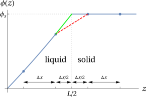
Figure 1: Enforcing the constant potential boundary condition (Dirichlet). The electrostatic potential is displayed as a function of position, in the vicinity of a solid electrode. For consistency with the hydrodynamic treatment, the liquid-solid interface is located halfway between two lattice nodes, as illustrated by the vertical dotted line at $z=L/2$. The resolution is $\Delta x$ and the reduced potential of the electrode is fixed at a constant value $\phi_{s}$. The ratio between the slopes of the thick (green) and dashed (red) lines is two. Unlike the former, the latter provides a poor estimation of the gradient at the interface, as illustrated by the figure. A consistent calculation of the gradient at the interface requires to account for this factor of two, which in turn leads to the modified Laplacian in Eq. II.3 as compared to Eq. 12. While $\phi$ is prescribed in the solid region, Poisson equation is solved in the liquid side.

In order to be consistent with this observation, we therefore propose a slightly modified algorithm: For each boundary link, i.e. such that ${\bf r}$ and ${\bf r}+{\bf c}_{i}\Delta t$ belong to different phases (interfacial nodes), we simply multiply by 2 the difference appearing in Eq. 12 when computing the Laplacian in Eq. 13 (in order to determine the potential on interfacial liquid nodes). The fact that this effectively places the boundary condition at the mid-plane is illustrated on Figure 1 in the case of a one-dimensional geometry. A related discussion can be found in Ref. 41, where the ion dynamics was simulated using finite elements (see their Eq. 15 seq.). The proposed modification applies this idea to the stencils used for differential operators consistent with the LB lattice (for a discussion of stencils in the bulk, see Ref. 56). It proves convenient to reformulate the modification in a compact form by introducing the characteristic function of the solid:

$$\chi_{s}({\bf r}) =\begin{cases}1&\text{if }{\bf r}\text{ is a solid node,}\\ 0&\text{if }{\bf r}\text{ is a fluid node.}\end{cases}$$ (14)

Eq. 12 is then replaced by:

$$\nabla^{2}\phi({\bf r}) =\frac{2}{c_{s}^{2}\Delta t^{2}}\sum_{i}w_{i}\left[\phi({\bf r}+{\bf c}_{i}\Delta t)-\phi({\bf r})\right]\times$$

$$\;\hskip 71.13188pt\left[1+\chi_{s}({\bf r}+{\bf c}_{i}\Delta t)-\chi_{s}({\bf r})\right]$$ (15)

when solving the Poisson equation via Eq. 13. A bona fide feature of this reformulation is that it is parametrization independent, and can be used for arbitrary geometry of the solid electrode. Note that this introduces a correction (with respect to Eq. 12) only at the boundaries, which can be shown using the above-mentioned Taylor expansion and sum rules to correspond to a surface term $2\nabla\phi({\bf r})\cdot\nabla\chi_{s}({\bf r})=-\frac{\sigma}{\epsilon_{0}\epsilon_{r}}{\bf n}$, with $\sigma$ the local surface charge density and ${\bf n}$ the local normal unit vector pointing out of the electrode (the factor of 2 again corresponds to the location of the interface between the solid and liquid nodes, as sketched in Fig. 1).

Once the potential distribution inside the liquid is known, in particular at the interfacial liquid nodes, we can compute the charge $Q$ of the electrodes using again the Poisson equation as:

$$Q =\Delta x^{3}\sum_{{\bf r}\in elec}\rho_{el}({\bf r})=-\frac{e\Delta x^{3}}{4\pi l_{B}}\sum_{{\bf r}\in elec}\nabla^{2}\phi({\bf r})$$ (16)

where the Laplacian is computed via Eq. II.3 and vanishes everywhere inside the electrode except at interfacial nodes, as expected for the charged induced by the polarization of a metal.

We will show in Section III that the method presented in this section allows to recover the correct potential throughout the liquid and in turn the correct ionic density profiles at steady-state, as well as the corresponding capacitance of the electrode with second order accuracy in the lattice spacing. As for the rest of the link-flux method, the discretization of the differential operators is only accurate for sufficiently small variations of the considered quantities (in particular of the potential) between neighboring nodes. We underline however that the voltage between electrodes needs not be small and that non-linear electrostatic regimes can be simulated using the present method provided that the lattice spacing is well chosen.

III Results and discussion

In the following, we validate our approach to impose constant-potential boundary conditions in LBE simulations by considering cases for which it is possible to obtain analytical results, in the linear regime. However the method can also be readily applied without this restriction. We consider two geometries, illustrated in Fig. 2, corresponding to parallel plate and cylindrical (coaxial) capacitors, with a 1:1 electrolyte ($z_{+}=-z_{-}=1$) at concentration $\rho_{s}$ corresponding to a Debye screening length $\lambda_{D}=\left(8\pi l_{B}\rho_{s}\right)^{-1/2}$. We assume for simplicity that both cations and anions have the same diffusion coefficient $D_{+}=D_{-}=D$, but the simulations can be readily performed without this restriction.

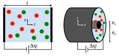
Figure 2: Capacitors consisting of an electrolyte confined between two metallic electrodes maintained at a constant potential difference $\Delta\psi$. Two geometries are considered: parallel plate capacitor (left), electrodes separated by a distance $L$ and coaxial capacitor (right) with electrodes of inner and outer radii $R_{1}$ and $R_{2}$. In the following we also consider the electro-osmotic flow induced in the charged capacitors by an additional electric field in the $y$ (resp. $z$) direction for the parallel plate (resp. coaxial) capacitor.

III.1 Parallel plate capacitor

We first consider parallel plate capacitors with two planar electrodes separated by a distance $L$ (in the $z$ direction, with $z=0$ at the mid-plane). Starting from an uncharged capacitor, we apply at $t=0$ a voltage $\Delta\psi=\psi_{2}-\psi_{1}=2.5$ mV between the two electrodes, or in reduced units (in terms of the thermal voltage $k_{B}T/e\approx 25$ mV): $\beta e\Delta\psi=0.1$. With such a small reduced voltage, it is possible to linearize the Poisson-Nernst-Planck equation to obtain the time-dependent charge on the positive electrode $Q(t)$ as well as the steady-state potential and ionic density profiles in the capacitor, which corresponds to the Debye-Hückel (DH) theory.

LBE simulations in this geometry are performed for a system with periodic boundary conditions in all directions, with $N_{x}=N_{y}=1$ in the directions parallel to the surfaces (this is sufficient to simulate infinite planar walls, as we checked by also performing simulations for $N_{x}=N_{y}=3$ for one of the systems). In the direction perpendicular to the electrodes we use $N_{z}=N_{f}+6$ nodes, where $N_{f}=L/\Delta x$ (with $L$ the distance between the solid/liquid interfaces and $\Delta x$ the lattice spacing) is the number of layers of fluid nodes, and 3 layers of nodes on each side of the liquid for the two electrodes. This choice ensures that there is no effect of the periodic boundary conditions in this direction on the charged induced at the surface of each electrode. We use a BGK relaxation $\tau=\Delta t$, which corresponds to a kinematic viscosity of $\nu=\frac{\eta}{\rho}=\frac{1}{6}\frac{\Delta x^{2}}{\Delta t}$. The diffusion coefficient of the ions is taken as $0.05\frac{\Delta x^{2}}{\Delta t}$, to ensure that the Schmidt number $Sc=\nu/D$ is larger than one, as for small ions in water (even though the order of magnitude is larger in this case). The potentials of the two electrodes are arbitrarily chosen as $\psi_{1}=0.1\leavevmode\nobreak\ k_{B}T/e$ and $\psi_{2}=0.2\leavevmode\nobreak\ k_{B}T/e$ to apply the desired voltage, but the resulting evolution of the ionic densities and electrode charge do not depend on the absolute potentials, as expected.

III.1.1 Potential and concentration profiles

Before examining the charge induced on the electrodes and the corresponding capacitance, we first examine the potential and concentration profiles through the capacitor, which are reported in Figure 3 for simulation parameters indicated in its caption. As explained above, the initial potential profile corresponds to the solution of the Poisson equation for a neutral capacitor, since the charge density vanishes inside the liquid because $\rho_{+}(z)=\rho_{-}(z)=\rho_{s}$ everywhere before the ions start moving. The corresponding initial electric field drives the cations and anions toward opposite electrodes. Once the electric double layers are established, there is no field in the bulk part of the liquid, i.e. at distances much larger than $\lambda_{D}$ (this can be achieved only in the regime $\lambda_{D}\ll L$).

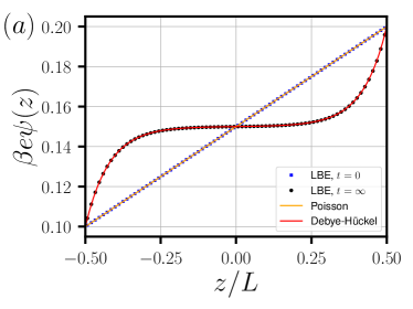
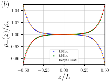
Figure 3: Steady-state electrostatic potential $\psi$ (a) and ionic concentration $\rho_{\pm}$ (b) profiles in a parallel capacitor, obtained from Lattice-Boltzmann Electrokinetics simulations (LBE, symbols) and Debye-Hückel theory (lines). Results are normalized by the thermal potential $k_{B}T/e$ and salt concentration $\rho_{s}$, respectively. In panel (a), we also indicate the initial potential profile: Right after establishing the potential drop and before the ions start to move, the fluid is neutral and the solution of the Poisson equation in this geometry is linear, as for a simple dielectric parallel plate capacitor. Simulations are performed for a separation $L=76\Delta x$, with a lattice spacing $\Delta x=l_{B}/1.44$, with $l_{B}$ the Bjerrum length, a salt concentration corresponding to a Debye length $\lambda_{D}=6\Delta x$, and a reduced voltage $\beta e\Delta\psi=0.1$.

The solution of the DH equation 5 for the parallel plate capacitor with boundary conditions $\psi(+L/2)=\psi_{2}$ and $\psi(-L/2)=\psi_{1}$ is given by:

$$\psi^{DH}(z) =\frac{\psi_{1}+\psi_{2}}{2}+\left(\frac{\psi_{2}-\psi_{1}}{2}\right)\times\frac{\sinh(\kappa z)}{\sinh(\kappa L/2)}\;.$$ (17)

Therefore in steady-state regime and the small voltage limit, both the potential and ionic density profiles decay exponentially from the surface, with a decay length $\lambda_{D}$. The LBE results are in excellent agreement with these analytical predictions in the considered range of physical and simulation parameters (which are the same as for Figure 4a). This is a first validation of the proposed method to impose the fixed potential boundary conditions.

III.1.2 Charge and capacitance

As explained in Section II.3, we can compute the instantaneous charge $Q(t)$ on the electrode surface from the potential distribution (once it has been determined from the ionic concentration via the Poisson equation) using Eq. 16. Figure 4a shows the charge as a function of time for a capacitor with electrodes separated by a distance $L\approx 52.8l_{B}\approx 36.9$ nm and electrolyte concentration (0.011 mol.L^-1) such that $\lambda_{D}\approx 4.2l_{B}\approx 2.9$ nm. The simulation parameters are indicated in the caption of the figure. The charge is reported normalized by the DH prediction for the surfacic capacitance:

$$C_{DH} =\epsilon_{0}\epsilon_{r}/2\lambda_{D}\;,$$ (18)

which can be interpreted physically as the capacitance for two parallel plate capacitors with distance $\lambda_{D}$ in series. Time is normalized by $L\lambda_{D}/2D$. The results nicely converge to the DH prediction, which is expected to be valid for such a small voltage and takes the form of Eq. 18 when $\lambda_{D}\ll L$. The charging dynamics will be analyzed in more detail in section III.1.3, but one can already note the exponential form of the charge as a function of time, illustrated by the solid line. Another point of interest is the initial value of the charge, which does not vanish once voltage is applied, but rather corresponds to the value for a dielectric (neutral) capacitor: $C_{0}=\epsilon_{0}\epsilon_{r}/L$. This is due to the fact that the liquid is neutral before the ions start moving (see the potential distribution inside the liquid in Figure 3a).

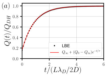
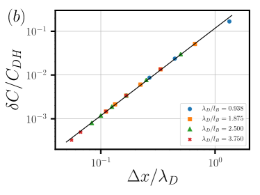
Figure 4: (a) Charging a parallel plate capacitor: The charge obtained from Lattice Boltzmann Electrokinetics (LBE) simulations, normalized by the Debye-Hückel prediction for the surfacic capacitance $C_{DH}=\epsilon_{0}\epsilon_{r}/2\lambda_{D}$, as a function of time normalized by $L\lambda_{D}/2D$. The initial value of the charge coincides with the expected value for a dielectric (neutral) capacitor $C_{0}=\epsilon_{0}\epsilon_{r}/L$. Simulations are performed for a separation $L=76\Delta x$, with a lattice spacing $\Delta x=l_{B}/1.44$, with $l_{B}$ the Bjerrum length, a salt concentration corresponding to a Debye length $\lambda_{D}=6\Delta x$, and a reduced voltage $\beta e\Delta\psi=0.1$. Results are shown only every 400 steps for clarity. The line shows an exponential fit of the LBE results (see Figure 5 for a discussion of the characteristic times), while horizontal and vertical lines are only guides for the eye. (b) Influence of the lattice spacing. The relative deviation of the simulated capacitance (computed from $Q_{\infty}$) with respect to the Debye-Hückel prediction is reported as a function of the ratio $\Delta x/\lambda_{D}$, for several salt concentrations corresponding to different ratios $\lambda_{D}/l_{B}$ and a fixed ratio $L/l_{B}=52.5$. The line has a slope of 2.

Of course, the accuracy of the simulation results depends on the level of discretization, more specifically the grid spacing $\Delta x$ with respect to the physical lengths. The latter are generally in the order $l_{B}<\lambda_{D}<L$, even though the order of the last two can be reversed for small electrolyte concentrations and distances between electrodes. The grid spacing must be sufficiently small to resolve the electric double layers at steady-state ($\Delta x/\lambda_{D}<1$).

Figure 4b shows the relative error on the steady-state capacitance with respect to the DH result as a function of $\Delta x/\lambda_{D}$, for a fixed ratio $L/l_{B}=52.5$ and several values of $\lambda_{D}/l_{B}$. The slope of 2 on this double logarithmic scale indicates that

$$\frac{|C_{LBE}-C_{DH}|}{C_{DH}} \propto\left(\frac{\Delta x}{\lambda_{D}}\right)^{2}\;,$$ (19)

for all considered cases, i.e. that our algorithm to impose constant-potential boundary conditions and to determine the surface charge induced by the ionic distributions in the electrolyte is accurate to second order. Note that we have pushed the numerical results to the rather extreme case of $\lambda_{D}\approx l_{B}$: this is a high concentration regime in which the DH theory itself becomes too crude an approximation, because correlations between ions (in particular due to excluded volume) cannot be neglected.

III.1.3 Charging dynamics

The LBE simulations do not only provide the steady-state electrode charge and potential/concentration profiles, but also their evolution with time. Figure 5a reports simulation results for the electrode charge similar to those of Figure 4a, at fixed salt concentration (0.065 mol.L^-1, corresponding to $\lambda_{D}=1.2$ nm) and resolution ($\Delta x/l_{B}$) but for several distances between electrodes $L$ (see caption for details) and in a scale that emphasizes the exponential relaxation of $Q(t)$ toward the steady-state solution. This scale clearly shows that the corresponding characteristic time (inverse of the slope) depends on the system.

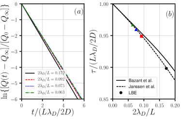
Figure 5: Charging dynamics in parallel plate capacitors. (a) Relaxation of the charge of the electrode $Q(t)$ from its initial value $Q_{0}$ to its final value $Q_{\infty}$, plotted on a logarithmic scale to illustrate the exponential decay, which allows to define a relaxation time $\tau$. (b) Relaxation time, normalized by the characteristic time $L\lambda_{D}/2D$, as a function of the ratio between the Debye screening length and the half-distance between the electrodes. Simulations are performed for several inter-electrode distances $L$, corresponding to the colors indicated in panel (a), with a lattice spacing $\Delta x=l_{B}/4.8$, with $l_{B}$ the Bjerrum length, a salt concentration corresponding to a Debye length $\lambda_{D}=8\Delta x$, and a reduced voltage $\beta e\Delta\psi=0.1$. The relaxation time for each $L$ is reported in panel (b) with the corresponding color. The simulations results are also compared to the analytical predictions in Eq. (36) of Ref. 20 and in Eq. (29) and preceding definitions of Ref. 21.

As pointed out e.g. by Bazant and coworkers Bazant, Thornton, and Ajdari (2004), the decay time is neither the Debye relaxation time $\lambda_{D}^{2}/D$, (which is the relaxation time for bulk electrolytes) corresponding to diffusion over the Debye length, nor the diffusion time over the distance $L$ between the electrodes, but rather $\sim L\lambda_{D}/2D$. More accurate analytical expressions have been derived in Ref. 20 and more recently by Janssen and Bier in Ref. 21, which include a correction of order $\lambda_{D}^{2}/D$. The result can be interpreted as an $RC$ charging time taking into account the capacitance of the electrode-electrolytes interfaces, estimated by $C_{DH}$, and the resistance of the bulk electrolyte, using the conductivity estimated via the Nernst-Einstein expression and considering a slab of width $\approx L-\lambda_{D}$ of electrolyte. The characteristic decay time $\tau$ is reported in Figure 5b, normalized by $L\lambda_{D}/2D$, as a function of the ratio $2\lambda_{D}/L$. The results are in perfect agreement with the results of Ref. 21, which also coincide with that of Ref. 20 for $\lambda_{D}\ll L$.

III.1.4 Electrokinetic effects

Finally, the LBE method is able to capture the electrokinetic coupling between the ions and the solvent. This is illustrated in the present case of constant-potential walls by examining the electro-osmotic response of the charged parallel plate capacitor (obtained as the steady-state of the previous sections) to an additional electric field $E_{y}$ parallel to the electrodes. Note that in a real system of a capacitor with finite lateral dimensions, such an additional field would be applied by other electrodes, located outside of the capacitor, and the field lines would be modified compared to the simplified case considered here for validation purposes. For sufficiently small applied field, the electro-osmotic flow is laminar and the steady-state solution of the Navier-Stokes equation 3 in this geometry, with no-slip boundary conditions and in the Debye-Hückel limit, is given by:

$$u_{y}(z) =\frac{\epsilon_{0}\epsilon_{r}E_{y}(\psi_{2}-\psi_{1})}{\eta}\times\frac{1}{2}\left(\frac{\sinh(\kappa z)}{\sinh(\kappa L/2)}-\frac{2z}{L}\right)$$ (20)

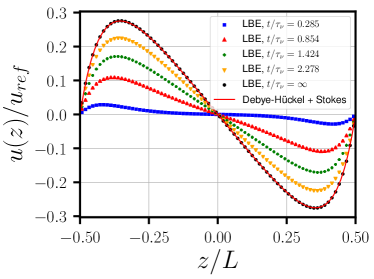
Figure 6: Electro-osmotic flow profile in a charged parallel capacitor, in the presence of an additional electric field $E_{y}$ along the electrodes. The situation at $t=0$ corresponds to the steady state of the charged capacitor. Lattice-Boltzmann Electrokinetics simulations (LBE) are shown with the symbols. The steady-state profile is compared to the theoretical result Eq. (20) combining Debye-Hückel theory for the electrostatic potential and the Stokes equation for the flow (line). Results are scaled with the reference velocity $u_{ref}=\epsilon_{0}\epsilon_{r}E_{y}(\psi_{2}-\psi_{1})/\eta$. Simulations are performed under the same conditions as in Figure 3, with a reduced applied field $\beta eE\Delta x=0.01$ parallel to the electrodes. The LBE simulations provide the time-dependence of the electrokinetic response, which reaches steady-state over a time scale $\tau_{\nu}=L^{2}/\pi^{2}\nu$ with $\nu=\eta/\rho$ the kinematic viscosity of the fluid, as expected from momentum diffusion in the direction perpendicular to the flow.

Figure 6 reports the simulation results corresponding to the system already shown in Figure 3 with an applied electric field in the $y$ direction of magnitude $\beta eE_{y}\Delta x=0.01$. It perfectly reproduces the analytical result expected to be valid for the considered range of physical parameters, which confirms the validity of the LBE scheme. We note that the resulting flow profile corresponds to shearing the fluid by applying opposite forces in the two double layers (since they are oppositely charged). This differs from the common situation of shear induced by moving walls in opposite directions, since the electrodes are not mobile in the present case.

This figure also shows electro-osmotic flow profiles in the transient regime. The flow builds up in the electric double layers near the electrodes and develops by momentum diffusion in the direction perpendicular to the electrodes, over a characteristic time scale $\tau_{\nu}=L^{2}/\pi^{2}\nu$ with $\nu=\eta/\rho$ the kinematic viscosity of the fluid.

As a final remark on the parallel plate capacitor, we emphasize again that the comparison is made here only in the linear regime where DH theory applies for validation purposes, but that the LBE simulations would provide the numerical solution of the non-linear PNP and Navier-Stokes outside of this regime.

III.2 Cylindrical (coaxial) capacitor

The setup to simulate cylindrical capacitors is illustrated in Figure 7. As for the parallel plate geometry, periodic boundary conditions along $z$ allow in principle to use a single lattice node in this direction to simulate an infinite system.

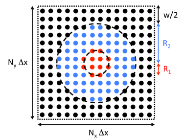
Figure 7: Simulation setup for the coaxial capacitor. The lattice consists of $N_{x}\times N_{y}\times N_{z}$ nodes with periodic boundary conditions in all directions (here a cut in the $xy$ plane is shown) at the boundaries of the box shown in dotted lines. The nodes corresponding to the fluid region, illustrated in blue, are located between two cylinders of radii $R_{1}$ (inner electrode, in red) and $R_{2}$ (outer electrode, in black) with potentials $\psi_{1}$ and $\psi_{2}$, respectively. All the region beyond the outer cylinder is maintained at the same potential (this defines the width $w$ of the electrode region as shown in the figure).

III.2.1 Potential profile

As for the parallel plate capacitor, we first examine the initial and steady-state potential profiles within the electrolyte. LBE simulations were performed in the setup illustrated in Figure 7, with a grid of $N_{x}\times N_{y}\times N_{z}=74\times 74\times 3$ nodes, a lattice spacing $\Delta x=l_{B}/1.2$, inner and outer cylinder radii of $R_{1}=2\Delta x\approx 1.2$ nm and $R_{2}=35\Delta x\approx 20.4$ nm, and a salt concentration ($\approx 0.0034$ mol.L^-1) corresponding to a screening length $\lambda_{D}=9\Delta x=7.5l_{B}\approx 5.25$ nm. With this choice of box size and outer radii, the width of the outer electrode region is $w=4\Delta x$, see Figure 7.

The potential satisfies the Poisson equation 2, with boundary conditions $\psi(R_{1})=\psi_{1}$ and $\psi(R_{2})=\psi_{2}$ as well as the constraint of opposite surface charge of the two cylinders leading to $R_{1}\psi^{\prime}(R_{1})=R_{2}\psi^{\prime}(R_{2})$. Before the ions start moving ($t=0$), the solution reads:

$$\psi_{0}^{cyl}(r) =\psi_{1}+(\psi_{2}-\psi_{1})\frac{\ln(r/R_{1})}{\ln(R_{2}/R_{1})}$$ (21)

with $r$ the radial distance from the axis of both cylindrical electrodes. Figure 8 shows that the initial potential profile obtained numerically with the SOR algorithm is in excellent agreement with this analytical solution, even though the inner cylinder is discretized quite roughly ($R_{1}=2\Delta x$ only). This further demonstrates the accuracy of our numerical scheme to impose constant-potential boundary conditions in a more complex geometry than planar electrodes.

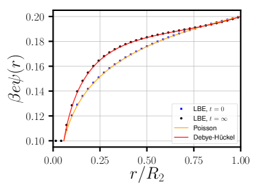
Figure 8: Electrostatic potential profile in a coaxial cylindrical channel, obtained from Lattice Boltzmann Electrokinetics simulations (LBE, symbols) and Debye-Hückel theory (line). We also indicate the initial potential profile: Before the ions start to move, the fluid is neutral and the solution of the Poisson equation in this geometry is the same as the one for a simple dielectric coaxial capacitor (see Eq.(21). Simulations are performed for an inner radius $R_{1}=2\Delta x$ and an outer radius $R_{2}=35\Delta x$, with a lattice spacing $\Delta x=l_{B}/1.2$, with $l_{B}$ the Bjerrum length, a salt concentration corresponding to a Debye length $\lambda_{D}=9\Delta x$, and a reduced voltage $\beta e\Delta\psi=0.1$ between the inner and outer electrodes.

Figure 8 also compares the LBE simulation results for the steady-state potential profile with the analytical solution of the DH equation 5 given by:

$$\psi_{DH}^{cyl}(r) =\psi_{1}+(\psi_{2}-\psi_{1})f(r,R_{1},R_{2},\kappa)$$ (22)

with:

$$f(r,R_{1},R_{2},\kappa) =\frac{\left[R_{2}{K_{1}(\kappa R_{2})}-R_{1}{K_{1}(\kappa R_{1})}\right]\left[{I_{0}(\kappa r)}-{I_{0}(\kappa R_{1})}\right]+\left[R_{2}{I_{1}(\kappa R_{2})}-R_{1}{I_{1}(\kappa R_{1})}\right]\left[{K_{0}(\kappa r)}-{K_{0}(\kappa R_{1})}\right]}{\left[R_{2}{K_{1}(\kappa R_{2})}-R_{1}{K_{1}(\kappa R_{1})}\right]\left[{I_{0}(\kappa R_{2})}-{I_{0}(\kappa R_{1})}\right]+\left[R_{2}{I_{1}(\kappa R_{2})}-R_{1}{I_{1}(\kappa R_{1})}\right]\left[{K_{0}(\kappa R_{2})}-{K_{0}(\kappa R_{1})}\right]}$$ (23)

where $I_{\alpha}$ and $K_{\alpha}$ are modified Bessel functions of the first and second kind. The LBE results are again in excellent agreement with the analytical DH predictions, which are expected to be valid in this low-voltage regime.

III.2.2 Capacitance

We now turn again to the charge induced on the electrode and corresponding capacitance. The electrode charge per unit length is coisnveniently derived using Gauss theorem from the electric field at the surface of the electrodes. Taking derivatives of the potential with respect to voltage $\psi_{2}-\psi_{1}$ and to the radial distance $r$ (evaluated at $r=R_{1}$), it follows from Eqs. 21 and 22-23 that the capacitances per unit length are: $C_{0}^{cyl}=2\pi\epsilon_{0}\epsilon_{r}/\ln(R_{2}/R_{1})$ for a neutral liquid (before the ions start moving) and:

$$C_{DH}^{cyl} =2\pi\epsilon_{0}\epsilon_{r}R_{1}f^{\prime}(R_{1},R_{1},R_{2},\kappa)$$ (24)

at steady-state (within the Debye-Hückel limit).

LBE simulations were performed in the setup illustrated in Figure 7, with a grid of $N_{x}\times N_{y}\times N_{z}=54\times 54\times 3$ node, inner and outer cylinder radii of $R_{1}=2\Delta x$ and $R_{2}=25\Delta x$, with a lattice spacing $\Delta x=l_{B}/1.2$. The reduced potential difference is again fixed to $\beta e\Delta\psi=0.1$ and the concentration is varied over a range corresponding to $\lambda_{D}/\Delta x=3$, 6, 9 and 12.

$\lambda_{D}/\Delta x$	$3$	$6$	$9$	$12$
$|C_{LBE}-C_{DH}^{cyl}|/C_{DH}^{cyl}$	2.3%	1.2%	1.0%	0.94%

Table 1: Relative error on the capacitance, computed at steady-state, with respect to the theoretical result Eq. 24 in the Debye-Hückel limit, for a coaxial capacitor (see text for simulation details).

Table 1 reports the relative errors for the capacitance computed at steady-state in the LBE simulations with respect to the Debye-Hückel analytical result 24 which is expected to be valid in this low-voltage regime. The errors are very small for the chosen range of simulation parameters. Similarly to the slit case, the error decreases as $(\Delta x/\lambda_{D})^{2}$ when the resolution of the double layer increases. However, the extrapolated value for $\Delta x/\lambda_{D}\to 0$ does not vanish in that case: This residual value ($\sim 0.8\%$) reflects other sources of errors, in particular due to the coarse discretization of the inner cylinder with a radius of only $R_{1}=2\Delta x$.

III.2.3 Electrokinetic effects

We finally examine the electrokinetic response of the charged coaxial capacitor to an additional electric field in the axial $z$ direction. The steady-state electro-osmotic flow profile can be derived from the Stokes equation using the steady-state potential profile, in the Debye-Hückel limit. The result for no-slip boundary conditions at the surface of the electrodes reads:

$$u_{z}(r) =\frac{\epsilon_{0}\epsilon_{r}E_{z}(\psi_{2}-\psi_{1})}{\eta}\left[f(r,R_{1},R_{2},\kappa)-\frac{\ln(r/R_{1})}{\ln(R_{2}/R_{1})}\right]$$ (25)

with $f$ given by Eq. 23.

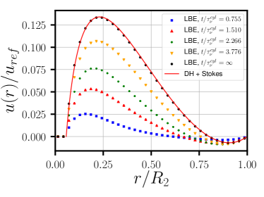
Figure 9: Electro-osmotic flow profile in a coaxial capacitor, in the presence of an additional electric field $E_{z}$ along the electrodes. The situation at $t=0$ corresponds to the steady state of the charged capacitor. Lattice-Boltzmann Electrokinetics simulations (LBE, symbols) for the steady-state are compared to the theoretical result Eq. (25) combining Debye-Hückel theory for the electrostatic potential and the Stokes equation for the flow (line). Results are scaled with the reference velocity $u_{ref}=\epsilon_{0}\epsilon_{r}E_{z}(\psi_{2}-\psi_{1})/\eta$ Simulations are performed under the same conditions as in Figure 8, with a reduced applied field $\beta eE_{z}\Delta x=0.0001$ parallel to the electrodes. The LBE simulations further provide the time-dependence of the electrokinetic response, which reaches steady-state over a time scale $\tau_{\nu}^{cyl}=(R_{2}-R_{1})^{2}/\pi^{2}\nu$. com

We performed LBE simulations with the same parameters as described in section III.2.1 for the potential profile. Starting from the charged capacitor, we apply a reduced electric field $\beta eE_{z}\Delta x=0.0001$ parallel to the electrodes (axial direction $z$) and monitor the velocity of the fluid in this direction, as a function of radial position $r$ and time $t$. The results shown in Figure 9 demonstrate that the steady-state velocity profile is in excellent agreement with the analytical result Eq. (25), as a last illustration of the validity of the proposed method to impose constant-potential boundary conditions. The transient regime (for which no analytical result is available) is consistent with the expected acceleration near the electrode surfaces, where the fluid is not neutral, followed by viscous momentum diffusion away from these regions to the whole fluid with a characteristic time $\propto(R_{2}-R_{1})^{2}/\nu$. com

As for the parallel plate capacitor, we note that the steady state corresponds to shearing the fluid via opposite forces within the two double layers. This results in particular in flows in opposite directions near the two electrodes, but with very different magnitudes in that case (larger velocity near the inner electrode) since the total fluid flux vanishes (there is no net force on the fluid which is overall neutral). Such an original setup may find applications to separate species in a mixture of ions.

IV Conclusion

We have introduced a simple rule to impose Dirichlet electrostatic boundary conditions in LBE simulations, in a consistent way with the location of the hydrodynamic interface (for stick boundary conditions), i.e. between the solid and liquid nodes rather than on the solid nodes. The proposed method also provides the instantaneous local charge induced on the electrode by the instantaneous distribution of ions under voltage. We validated it in the low voltage regime by comparison with analytical results in two model capacitors (parallel plate and coaxial electrodes), examining the steady-state ionic concentrations and electric potential profiles, the time-dependent response of the charge on the electrodes, as well as the steady-state electro-osmotic profiles in the presence of an additional, tangential electric field. The LBE method naturally provides the time-dependence of all these quantities – a possibility that we illustrate on the electro-osmotic response. While we do not consider this case in the present work, which focuses on the validation of the method, the latter readily applies to large voltages between the electrodes, as well as to time-dependent voltages. The only restriction is a sufficiently small lattice spacing, with small potential differences (compared to $k_{B}T/e$) between neighboring nodes. Besides, we have shown that the method is accurate to second order in lattice spacing.

This work opens the way to the LBE simulation of more complex systems involving electrodes and metallic surfaces, such as the nanofluidic channels and nanotubes mentioned in the introduction, or porous electrodes, since the algorithm can readily be applied to arbitrary geometries. It would also be a convenient tool for the simulation of other electrokinetic phenomena, such as induced-charged electrokineticsBazant and Squires (2010). On the methodological side, possible extensions include the coupling of electrokinetics to adsorption/desorption at the solid-liquid interfaceLevesque et al. (2013); Vanson et al. (2015); Asta, Levesque, and Rotenberg (2018), which may play a role in the specific behavior of carbon vs boron nitride nanotubesGrosjean et al. (2016), as well as including additional excess terms in the free energy model underlying the present work (which only leads to the emergence of the Nernst-Planck dynamics for the ions). In particular, capturing the effect of ion correlationsStorey and Bazant (2012) would be necessary to simulate more concentrated electrolytes as well as multivalent ions. Finally, it would be useful to obtain analytical results in the non-linear regime, at least in simple geometries, in order to validate the numerical method outside of the range considered here. Work in this direction is in progress.

References

- Blase et al. (1994) X. Blase, L. X. Benedict, E. L. Shirley, and S. G. Louie, “Hybridization effects and metallicity in small radius carbon nanotubes,” Physical Review Letters 72, 1878–1881 (1994).
- Rassaei et al. (2012) L. Rassaei, K. Mathwig, E. D. Goluch, and S. G. Lemay, “Hydrodynamic Voltammetry with Nanogap Electrodes,” The Journal of Physical Chemistry C 116, 10913–10916 (2012).
- Mathwig and Lemay (2013) K. Mathwig and S. G. Lemay, “Pushing the Limits of Electrical Detection of Ultralow Flows in Nanofluidic Channels,” Micromachines 4, 138–148 (2013).
- Lemay et al. (2013) S. G. Lemay, S. Kang, K. Mathwig, and P. S. Singh, “Single-molecule electrochemistry: present status and outlook,” Accounts of Chemical Research 46, 369–377 (2013).
- Sun and Mirkin (2008) P. Sun and M. V. Mirkin, “Electrochemistry of Individual Molecules in Zeptoliter Volumes,” Journal of the American Chemical Society 130, 8241–8250 (2008).
- Bocquet and Charlaix (2010) L. Bocquet and E. Charlaix, “Nanofluidics, from bulk to interfaces,” Chemical Society Reviews 39, 1073–1095 (2010).
- Siria et al. (2013) A. Siria, P. Poncharal, A.-L. Biance, R. Fulcrand, X. Blase, S. T. Purcell, and L. Bocquet, “Giant osmotic energy conversion measured in a single transmembrane boron nitride nanotube,” Nature 494, 455–458 (2013).
- Secchi et al. (2016) E. Secchi, A. Niguès, L. Jubin, A. Siria, and L. Bocquet, “Scaling Behavior for Ionic Transport and its Fluctuations in Individual Carbon Nanotubes,” Physical Review Letters 116, 154501 (2016).
- Jubin et al. (2018) L. Jubin, A. Poggioli, A. Siria, and L. Bocquet, “Dramatic pressure-sensitive ion conduction in conical nanopores,” Proceedings of the National Academy of Sciences , 201721987 (2018).
- Gouy (1910) G. Gouy, J. Phys. Theor. Appl 9, 457 (1910).
- Chapman (1913) D. Chapman, Phil. Mag. 25, 475 (1913).
- Stern (1924) O. Stern, Z. Elektrochem. 30, 508 (1924).
- Grün et al. (2004) F. Grün, M. Jardat, P. Turq, and C. Amatore, “Relaxation of the electrical double layer after an electron transfer approached by Brownian dynamics simulation,” The Journal of Chemical Physics 120, 9648–9655 (2004).
- Siepmann and Sprik (1995) J. I. Siepmann and M. Sprik, “Influence of surface topology and electrostatic potential on water/electrode systems,” The Journal of Chemical Physics 102, 511–524 (1995).
- Reed, Lanning, and Madden (2007) S. K. Reed, O. J. Lanning, and P. A. Madden, “Electrochemical interface between an ionic liquid and a model metallic electrode,” The Journal of Chemical Physics 126, 084704 (2007).
- Merlet et al. (2013a) C. Merlet, B. Rotenberg, P. A. Madden, and M. Salanne, “Computer simulations of ionic liquids at electrochemical interfaces,” Physical Chemistry Chemical Physics 15, 15781–15792 (2013a).
- Merlet et al. (2013b) C. Merlet, C. Péan, B. Rotenberg, P. A. Madden, P. Simon, and M. Salanne, “Simulating Supercapacitors: Can We Model Electrodes As Constant Charge Surfaces?” The Journal of Physical Chemistry Letters 4, 264–268 (2013b).
- Limmer et al. (2013) D. T. Limmer, C. Merlet, M. Salanne, D. Chandler, P. A. Madden, R. van Roij, and B. Rotenberg, “Charge Fluctuations in Nanoscale Capacitors,” Physical Review Letters 111, 106102 (2013).
- Merlet et al. (2014) C. Merlet, D. T. Limmer, M. Salanne, R. van Roij, P. A. Madden, D. Chandler, and B. Rotenberg, “The Electric Double Layer Has a Life of Its Own,” The Journal of Physical Chemistry C 118, 18291–18298 (2014).
- Bazant, Thornton, and Ajdari (2004) M. Z. Bazant, K. Thornton, and A. Ajdari, “Diffuse-charge dynamics in electrochemical systems,” Physical Review E 70, 021506 (2004).
- Janssen and Bier (2018) M. Janssen and M. Bier, “Transient dynamics of electric double layer capacitors: Exact expressions within the Debye-Falkenhagen approximation,” Physical Review E 97, 052616 (2018).
- Biesheuvel and Bazant (2010) P. M. Biesheuvel and M. Z. Bazant, “Nonlinear dynamics of capacitive charging and desalination by porous electrodes,” Physical Review E 81, 031502 (2010).
- Joly et al. (2004) L. Joly, C. Ybert, E. Trizac, and L. Bocquet, “Hydrodynamics within the Electric Double Layer on Slipping Surfaces,” Physical Review Letters 93, 257805 (2004).
- Joly et al. (2006) L. Joly, C. Ybert, E. Trizac, and L. Bocquet, “Liquid friction on charged surfaces: From hydrodynamic slippage to electrokinetics,” The Journal of Chemical Physics 125, 204716–204716–14 (2006).
- Yoshida et al. (2014) H. Yoshida, H. Mizuno, T. Kinjo, H. Washizu, and J.-L. Barrat, “Molecular dynamics simulation of electrokinetic flow of an aqueous electrolyte solution in nanochannels,” The Journal of Chemical Physics 140, 214701 (2014).
- Pagonabarraga, Rotenberg, and Frenkel (2010) I. Pagonabarraga, B. Rotenberg, and D. Frenkel, “Recent advances in the modelling and simulation of electrokinetic effects: bridging the gap between atomistic and macroscopic descriptions,” Phys. Chem. Chem. Phys. 12, 9566–9580 (2010).
- Rotenberg and Pagonabarraga (2013) B. Rotenberg and I. Pagonabarraga, “Electrokinetics: insights from simulation on the microscopic scale,” Molecular Physics 111, 827–842 (2013).
- Smiatek et al. (2009) J. Smiatek, M. Sega, C. Holm, U. D. Schiller, and F. Schmid, “Mesoscopic simulations of the counterion-induced electro-osmotic flow: A comparative study,” The Journal of Chemical Physics 130, 244702 (2009).
- Ceratti et al. (2015) D. R. Ceratti, A. Obliger, M. Jardat, B. Rotenberg, and V. Dahirel, “Stochastic rotation dynamics simulation of electro-osmosis,” Molecular Physics 113, 2476–2486 (2015).
- Dahirel et al. (2018) V. Dahirel, X. Zhao, B. Couet, G. Batôt, and M. Jardat, “Hydrodynamic interactions between solutes in multiparticle collision dynamics,” Physical Review E 98, 053301 (2018).
- Succi (2001) S. Succi, The Lattice Boltzmann Equation for Fluid Dynamics and Beyond (Oxford University Press, 2001).
- Lobaskin, Dünweg, and Holm (2004) V. Lobaskin, B. Dünweg, and C. Holm, “Electrophoretic mobility of a charged colloidal particle: a computer simulation study,” Journal of Physics: Condensed Matter 16, S4063 (2004).
- Lobaskin et al. (2007) V. Lobaskin, B. Dünweg, M. Medebach, T. Palberg, and C. Holm, “Electrophoresis of Colloidal Dispersions in the Low-Salt Regime,” Physical Review Letters 98, 176105 (2007).
- Hickey et al. (2010) O. A. Hickey, C. Holm, J. L. Harden, and G. W. Slater, “Implicit Method for Simulating Electrohydrodynamics of Polyelectrolytes,” Physical Review Letters 105, 148301 (2010).
- Hickey and Holm (2013) O. A. Hickey and C. Holm, “Electrophoretic mobility reversal of polyampholytes induced by strong electric fields or confinement,” The Journal of Chemical Physics 138, 194905 (2013).
- Datar et al. (2017) A. V. Datar, M. Fyta, U. M. B. Marconi, and S. Melchionna, “Electrokinetic Lattice Boltzmann Solver Coupled to Molecular Dynamics: Application to Polymer Translocation,” Langmuir 33, 11635–11645 (2017).
- Lobaskin and Netz (2016) V. Lobaskin and R. R. Netz, “Diffusive-convective transition in the non-equilibrium charging of an electric double layer,” EPL (Europhysics Letters) 116, 58001 (2016).
- Marini Bettolo Marconi and Melchionna (2012) U. Marini Bettolo Marconi and S. Melchionna, “Charge Transport in Nanochannels: A Molecular Theory,” Langmuir 28, 13727–13740 (2012).
- Wang, Wang, and Li (2006) J. Wang, M. Wang, and Z. Li, “Lattice Poisson-Boltzmann simulations of electro-osmotic flows in microchannels,” Journal of Colloid and Interface Science 296, 729–736 (2006).
- Thakore and Hickman (2015) V. Thakore and J. J. Hickman, “Charge Relaxation Dynamics of an Electrolytic Nanocapacitor,” The Journal of Physical Chemistry C 119, 2121–2132 (2015).
- Hlushkou, Kandhai, and Tallarek (2004) D. Hlushkou, D. Kandhai, and U. Tallarek, “Coupled lattice-Boltzmann and finite-difference simulation of electroosmosis in microfluidic channels,” International Journal for Numerical Methods in Fluids 46, 507–532 (2004).
- Hlushkou et al. (2007) D. Hlushkou, S. Khirevich, V. Apanasovich, A. Seidel-Morgenstern, and U. Tallarek, “Pore-Scale Dispersion in Electrokinetic Flow through a Random Sphere Packing,” Analytical Chemistry 79, 113–121 (2007).
- Hlushkou et al. (2016) D. Hlushkou, K. N. Knust, R. M. Crooks, and U. Tallarek, “Numerical simulation of electrochemical desalination,” Journal of Physics: Condensed Matter 28, 194001 (2016).
- Warren (1997) P. B. Warren, “Electroviscous transport problems via Lattice-Boltzmann,” International Journal of Modern Physics C 8, 889 (1997).
- Horbach and Frenkel (2001) J. Horbach and D. Frenkel, “Lattice-Boltzmann method for the simulation of transport phenomena in charged colloids,” Physical Review E 64, 061507 (2001).
- Capuani, Pagonabarraga, and Frenkel (2004) F. Capuani, I. Pagonabarraga, and D. Frenkel, “Discrete solution of the electrokinetic equations,” The Journal of Chemical Physics 121, 973–986 (2004).
- Rotenberg, Pagonabarraga, and Frenkel (2008) B. Rotenberg, I. Pagonabarraga, and D. Frenkel, “Dispersion of charged tracers in charged porous media,” EPL (Europhysics Letters) 83, 34004 (2008).
- Pagonabarraga, Capuani, and Frenkel (2005) I. Pagonabarraga, F. Capuani, and D. Frenkel, “Mesoscopic lattice modeling of electrokinetic phenomena,” Computer Physics Communications Proceedings of the Europhysics Conference on Computational Physics 2004, 169, 192–196 (2005).
- Capuani, Pagonabarraga, and Frenkel (2006) F. Capuani, I. Pagonabarraga, and D. Frenkel, “Lattice-Boltzmann simulation of the sedimentation of charged disks,” The Journal of Chemical Physics 124, 124903–124903–11 (2006).
- Giupponi and Pagonabarraga (2011) G. Giupponi and I. Pagonabarraga, “Colloid Electrophoresis for Strong and Weak Ion Diffusivity,” Physical Review Letters 106, 248304 (2011).
- Rempfer et al. (2016) G. Rempfer, G. B. Davies, C. Holm, and J. d. Graaf, “Reducing spurious flow in simulations of electrokinetic phenomena,” The Journal of Chemical Physics 145, 044901 (2016).
- Kuron et al. (2016) M. Kuron, G. Rempfer, F. Schornbaum, M. Bauer, C. Godenschwager, C. Holm, and J. de Graaf, “Moving charged particles in lattice Boltzmann-based electrokinetics,” The Journal of Chemical Physics 145, 214102 (2016).
- Rotenberg, Frenkel, and Pagonabarraga (2010) Rotenberg, D. Frenkel, and Pagonabarraga, “Coarse-grained simulations of charge, current and flow in heterogeneous media,” Faraday Discuss. 144, 9–24 (2010).
- Rivas et al. (2018) N. Rivas, S. Frijters, I. Pagonabarraga, and J. Harting, “Mesoscopic electrohydrodynamic simulations of binary colloidal suspensions,” The Journal of Chemical Physics 148, 144101 (2018).
- Obliger et al. (2013) A. Obliger, M. Duvail, M. Jardat, D. Coelho, S. Békri, and B. Rotenberg, “Numerical homogenization of electrokinetic equations in porous media using lattice-Boltzmann simulations,” Physical Review E 88, 013019 (2013).
- Thampi, Pagonabarraga, and Adhikari (2011) S. P. Thampi, I. Pagonabarraga, and R. Adhikari, “Lattice-Boltzmann-Langevin simulations of binary mixtures,” Physical Review E 84, 046709 (2011).
- (57) The exact expression for the largest momentum relaxation time is . The value of is determined by the following equation: , where and are Bessel functions of the first and second kind. Here, is 0.867 and, in general, a numerical solution of the equation shows that .
- Bazant and Squires (2010) M. Z. Bazant and T. M. Squires, “Induced-charge electrokinetic phenomena,” Current Opinion in Colloid & Interface Science 15, 203–213 (2010).
- Levesque et al. (2013) M. Levesque, M. Duvail, I. Pagonabarraga, D. Frenkel, and B. Rotenberg, “Accounting for adsorption and desorption in lattice Boltzmann simulations,” Physical Review E 88, 013308 (2013).
- Vanson et al. (2015) J.-M. Vanson, F. c.-X. Coudert, B. Rotenberg, M. Levesque, C. Tardivat, M. Klotz, and A. Boutin, “Unexpected coupling between flow and adsorption in porous media,” Soft Matter 11, 6125–6133 (2015).
- Asta, Levesque, and Rotenberg (2018) A. Asta, M. Levesque, and B. Rotenberg, “Moment propagation method for the dynamics of charged adsorbing/desorbing species at solid-liquid interfaces,” Molecular Physics 116, 2965–2976 (2018).
- Grosjean et al. (2016) B. Grosjean, C. Pean, A. Siria, L. Bocquet, R. Vuilleumier, and M.-L. Bocquet, “Chemisorption of Hydroxide on 2d Materials from DFT Calculations: Graphene versus Hexagonal Boron Nitride,” The Journal of Physical Chemistry Letters 7, 4695–4700 (2016).
- Storey and Bazant (2012) B. D. Storey and M. Z. Bazant, “Effects of electrostatic correlations on electrokinetic phenomena,” Physical Review E 86, 056303 (2012).