Cooperative Localization with Angular Measurements and Posterior Linearization

Abstract

The application of cooperative localization in vehicular networks is attractive to improve accuracy and coverage. Conventional distance measurements between vehicles are limited by the need for synchronization and provide no heading information of the vehicle. To address this, we present a cooperative localization algorithm using posterior linearization belief propagation (PLBP) utilizing angle-of-arrival (AoA)-only measurements. Simulation results show that both directional and positional root mean squared error (RMSE) of vehicles can be decreased significantly and converge to a low value in a few iterations. Furthermore, the influence of parameters for the vehicular network, such as vehicle density, communication radius, prior uncertainty and AoA measurements noise, is analyzed.

I Introduction

Vehicular localization with high precision is of great importance for future autonomous driving. Among different possibilities, e.g., global navigation satellite system (GNSS) [1], cooperative localization [2] enables the possibility for message passing (MP) between vehicles, which can lead to more accurate positioning and increased positioning coverage. In cooperative localization, vehicles use on-board sensors, including 5G front-end, radar and stereo cameras [3], to obtain measurements relative to the positions of nearby vehicles. Vehicles exchange information related to relative positions and own position estimates to obtain an approximation of their own posterior distribution. Belief propagation (BP) [4] is a well-known framework for Bayesian inference that can be applied for the cooperative localization problem [2]. Cooperative localization is particularly advantageous when vehicles have different prior localization accuracy, because vehicles with high-quality sensors can help vehicles with low quality sensors to reduce their localization errors. The last point is practical in the foreseeable future because vehicles with different levels of sensing precision are expected to coexist[5].

Figure 1: Geometric model of two vehicles. Vehicle $i$ measures the AoA $[\mathbf{h}_{ij}(\mathbf{x}_{ij})]_{1}$ from vehicle $j$, and vehicle $j$ measures $[\mathbf{h}_{ij}(\mathbf{x}_{ij})]_{2}$.

The performance of any localization system is limited by the underlying measurements. Conventional measurements include distance and angle between vehicles. In terms of distance measurements, radar can provide high accuracy, but does not include identity information of the target, required for MP. Measurements based on the travel time of radio signals ( time-of-arrival (TOA) and time-difference-of-arrival (TDOA)) can provide such identity information [6, 7, 8]. However, TOA and TDOA are challenged by the synchronization requirements [7]. The clocks of two vehicles need to be synchronized such that the delay can be computed. This can lead to significant localization error because of small clock error [9], or to use two-way TOA with round-trip delay time instead of the one-way delay to avoid synchronization, which doubles the resource requirement. Achieving a ranging accuracy lower than 10 m by TOA/TDOA is very challenging in vehicular environments [10]. In contrast, AoA is readily available when the receiver is equipped with an antenna array [11, 12, 13, 14]: [13] has investigated the performance of vehicle-to-vehicle (V2V) relative positioning using AoA measurements from multiple receiving arrays on the vehicle, and the achieved positioning accuracy met requirements of 5G New Radio (NR) vehicle-to-everything (V2X) standardization. While AoA measurements are attractive from a practical point of view, the integration in MP is non-trivial. Due to the nonlinear relation between the AoA and the vehicle state, analytical computation of the messages in BP is not possible. Approximations include the use of particles [15, 16] or linearization of the measurement model [17]. While the increasing number of particles gives better approximation performance, it also increases the computation complexity. To address this problem, [14] uses a von Mises-Fisher (VMF) model for the measurement likelihood and performs PLBP [18], for a scenario with unknown positions but known orientation.

In this paper, we consider a cooperative localization problem where vehicles’ positions and orientations are unknown. We apply Gaussian parametric BP [19] for the MP, which reduces the communication resource overhead and computational complexity compared to a particle approach. To pass those messages through the nonlinear angle measurement model, posterior linearization (PL) [18] is applied to linearize the model using statistical linear regression (SLR) with respect to the posterior, which can be calculated by the current messages [20]. Based on the linearized model, the BP is then performed to update the new beliefs. This PLBP procedure can be iterated so that the posterior probability density function (PDF) of the vehicle position and orientation can converge.

II Problem Statement

We consider a network comprising a set of vehicles $\mathcal{V}=\{1,...,N\}$. A set of communication links $\mathcal{E}\subset\mathcal{V}\times\mathcal{V}$ are considered to connect each vehicle according to a communication radius $r$. The neighbor set of vehicle $i$ is denoted by $\mathcal{N}_{i}$. Each vehicle $i\in\mathcal{V}$ has a state $\mathbf{x}_{i}\in\mathbb{R}^{3}$, comprising the 2D position $[x_{i},y_{i}]^{\mathsf{T}}$ and the heading $\theta_{i}\in(-\pi,\pi]$. We denote the joint state of vehicles $i$ and $j$ as $\mathbf{x}_{ij}=[\mathbf{x}^{\mathsf{T}}_{i}\mathbf{x}^{\mathsf{T}}_{j}]^{\mathsf{T}}$. Each vehicle is assumed to have knowledge of its prior state by some accessible positioning techniques, e.g., GNSS, assumed to be a Gaussian density

$$p_{i}(\mathbf{x}_{i})=\mathcal{N}(\mathbf{x}_{i};\bm{\mu}_{i},\mathbf{P}_{i}),$$ (1)

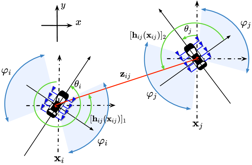
where $\mathcal{N}(\mathbf{x}_{i};\bm{\mu}_{i},\mathbf{P}_{i})$ denotes a Gaussian distribution in variable $\mathbf{x}_{i}$ with mean vector $\bm{\mu}_{i}=[\mu_{x},\mu_{y},\mu_{\theta}]^{\intercal}$ and covariance matrix $\mathbf{P}_{i}$. The measurement model between two vehicles is shown in Fig. 1. Each vehicle $i$ is equipped with linear arrays on its two sides, each of which provides a field of view (FOV) $\varphi_{i}$ with $0<\varphi_{i}\leq\pi$. Signals with an AoA measurements within the FOV of node can be measured. The AoA measurement vector $\mathbf{z}_{ij}$ between vehicles $i$ and $j$ is defined as a function of $\mathbf{x}_{i}$ and $\mathbf{x}_{j}$ with additive Gaussian noise

$$\mathbf{z}_{ij}=\mathbf{h}_{ij}(\mathbf{x}_{ij})+\bm{\eta}_{ij},$$ (2)

where $\bm{\eta}_{ij}$ represents the measurement noise, modeled as $\bm{\eta}_{ij}\sim\mathcal{N}(\mathbf{0},\mathbf{R}_{ij})$ and $\mathbf{h}_{ij}(\mathbf{x}_{ij})$ is defined as

$$\mathbf{h}_{ij}(\mathbf{x}_{ij})=\left[\begin{array}[]{c}\operatorname{atan2}\left((y_{j}-y_{i}),(x_{j}-x_{i})\right)-\theta_{i}\\ \operatorname{atan2}((y_{i}-y_{j}),(x_{i}-x_{j}))-\theta_{j}\end{array}\right],$$ (5)

in which $\operatorname{atan2}(y,x)$ calculate the four-quadrant inverse tangent of $y$ and $x$. However, the $\operatorname{atan2}$ introduces problems because of its discontinuity at the negative semi-axis of $x$, i.e. $(x,0):x<0$. Instead of modeling the angular measurements by VMF distribution, as [14] has done, we adopt a simple ad-hoc correction from [22], which is described in Appendix A. We denote the vector of all measurements by $\mathbf{z}=[\mathbf{z}_{ij}]_{i,j\in\mathcal{N}_{i}}$ and the vector of all vehicles’ states by $\mathbf{x}$. The goal of the network is to compute $p_{i}(\mathbf{x}_{i}|\mathbf{z})$, for each vehicle.

III Belief Propagation and Posterior Linearization

III-A Belief Propagation Formulation

The standard approach to solve the localization problem is to use belief propagation. We first factorize the joint PDF

$$p(\mathbf{x},\mathbf{z}) =p(\mathbf{x})p(\mathbf{z}|\mathbf{x})$$ (6)

$$=\prod_{i=1}^{N}p_{i}(\mathbf{x}_{i})\prod_{j\in\mathcal{N}_{i},j>i}p(\mathbf{z}_{ij}|\mathbf{x}_{ij}).$$ (7)

A factor graph representation of this joint PDF in combination with loopy BP allows the computation of approximations of the marginal posteriors $p_{i}(\mathbf{x}_{i}|\mathbf{z})$. The BP message passing rules at iteration $k$ are as follows (assuming $j\in\mathcal{N}_{i}$)[4]

$$b_{j}^{(k-1)}(\mathbf{x}_{j}) \propto p_{j}(\mathbf{x}_{j})\prod_{i\in\mathcal{N}_{j}}m^{(k-1)}_{i\to j}(\mathbf{x}_{j})$$ (8)

$$m^{(k)}_{j\to i}(\mathbf{x}_{i}) \propto\int p(\mathbf{z}_{ij}|\mathbf{x}_{ij})\frac{b_{j}^{(k-1)}(\mathbf{x}_{j})}{m^{(k-1)}_{i\to j}(\mathbf{x}_{j})}\text{d}\mathbf{x}_{j}.$$ (9)

The approximate marginal posterior at iteration $k$ is $p_{j}(\mathbf{x}_{j}|\mathbf{z})\approx b_{j}^{(k)}(\mathbf{x}_{j})$. The process is initialized at $k=0$ by $b_{j}^{(0)}(\mathbf{x}_{j})=p_{j}(\mathbf{x}_{j})$ and $m^{(0)}_{i\to j}(\mathbf{x}_{j})=1$. The joint posterior of $\mathbf{x}_{i},\mathbf{x}_{j}$ can also be approximated by[4]

$$b^{(k)}(\mathbf{x}_{ij}) \propto p(\mathbf{z}_{ij}|\mathbf{x}_{ij})\frac{b_{i}^{(k)}(\mathbf{x}_{i})b_{j}^{(k)}(\mathbf{x}_{j})}{m^{(k)}_{i\to j}(\mathbf{x}_{j}){m^{(k)}_{j\to i}(\mathbf{x}_{i})}}.$$ (10)

However, due to the nonlinear observation model (2), in general BP cannot be executed in closed form: neither the integral (8) nor the product (9) can be computed exactly, except when the observation model is linear with Gaussian noise [18]. This motivates the following linearization procedure.

III-B Linearization

Given a belief $b^{(k)}(\mathbf{x}_{ij})$, we approximate the observation model by

$$\mathbf{h}_{ij}(\mathbf{x}_{ij}) \approx\mathbf{C}_{ij}\tilde{\mathbf{x}}_{ij}+\mathbf{e}_{ij},$$ (11)

where $\mathbf{e}_{ij}\sim\mathcal{N}(\mathbf{0},\bm{\Omega}_{i,j})$, and $\tilde{\mathbf{x}}_{ij}=[{\mathbf{x}}^{\mathsf{T}}_{ij}~{}\mathbf{1}^{\mathsf{T}}]^{\mathsf{T}}$. $\mathbf{C}_{ij}$ is selected to minimize the mean square error (MSE) over the given joint belief $b^{(k)}(\mathbf{x}_{ij})$:

$$\arg\underset{\mathbf{C}_{ij}}{\min} ~{}\mathbb{E}\{\|\mathbf{h}_{ij}(\mathbf{x}_{ij})-\mathbf{C}_{ij}\tilde{\mathbf{x}}_{ij}\|^{2}\}.$$ (12)

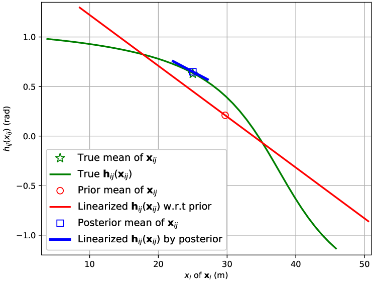
Once $\mathbf{C}_{ij}$ is determined, we find that $\bm{\Omega}_{i,j}=\|\mathbf{h}_{ij}(\mathbf{x}_{ij})-\mathbf{C}_{ij}\tilde{\mathbf{x}}_{ij}\|^{2}$. To solve this optimization problem, the SLR [18] with respect to the posterior PDF is performed, where the details are presented in Appendix A. To visualize the advantage of posterior SLR, Fig. 2 shows the true measurement model (5) and its approximations (11) with respect to posterior and prior. We observe that the linearized model by posterior SLR is more accurate and has less uncertainty than the model linearized by prior SLR.

Figure 2: The true measurement model $\mathbf{h}_{ij}(\mathbf{x}_{ij})$ and its approximations by SLR with respect to the prior and posterior, as a function of the $x$-dimension of $\mathbf{x}_{i}$. The length of the red and blue lines represent 2 standard deviations of the prior and posterior linearized models, respectively.

III-C Belief Propagation with Linearized Measurement Models

Once a linearization of all measurement models is obtained, BP is performed as follows. The likelihood function is now of the form

$$p(\mathbf{z}_{ij}|\mathbf{x}_{ij})\propto$$ (13)

$$\exp\left(-\frac{1}{2}(\mathbf{z}_{ij}-\mathbf{C}_{ij}\tilde{\mathbf{x}}_{ij})^{\mathsf{T}}\bm{\Sigma}^{-1}_{ij}(\mathbf{z}_{ij}-\mathbf{C}_{ij}\tilde{\mathbf{x}}_{ij})\right),$$

where $\bm{\Sigma}_{ij}=\bm{\Omega}_{ij}+\mathbf{R}_{ij}$. This formulation now allows closed-form Gaussian message passing according to (8)–(9) and (10). The details of the implementation are provided in the Appendix B.

The overall algorithm thus operates as described in Algorithm 1. The algorithm requires a selection of $K$ (the number of linearization iterations) and $M$ (the number of BP iterations per linearization step). The overall complexity per vehicle is approximately $\mathcal{O}(KM\bar{N}D^{3})$, where $D$ is the state dimension and $\bar{N}$ is the average number of neighbors.

Algorithm 1 : Iterative Cooperative Localization

  for $k=1$ to $K$ do

     Given the current beliefs $b^{(k-1)}(\mathbf{x}_{ij})$, solve (12) for each $(i,j)\in\mathcal{E}$ to obtain (13).

     Run $M$ iterations of BP on the linearized model.

     Compute joint beliefs $b^{(k)}(\mathbf{x}_{ij})$ at the current BP iteration.

  end for

  Return marginal beliefs.

IV Simulation Results

In this section we simulated a vehicular network scenario and analyzed the performance of the designed Algorithm 1. First, the localization and orientation performance of Algorithm 1 in the vehicle network is evaluated by the positional and directional RMSE. Then, based on this scenario, we analyzed the impact of different network parameters.

IV-A Simulation Scenario

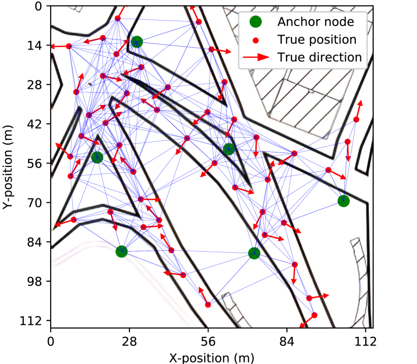
The vehicular scenario is based on a road map in central New York Manhattan (latitude: $40.71590$ and longitude: $-73.99560$). The map data is generated from Stamen Map [23] at a zoom level of 18. Within this map, the scenario is shown in Fig. 3, where 51 vehicles are possibly connected within the communication radius ($r=30~{}\text{m}$). The priors are set to $\mathbf{P}_{i}=\text{diag}(\sigma^{2}_{x},\sigma^{2}_{y},\sigma^{2}_{\theta})$. Among the vehicles, 6 are chosen as anchors (vehicles or road side units with a very concentrated prior density, set to $\text{diag}(\sigma_{x}^{2},\sigma_{y}^{2},\sigma_{\theta}^{2})=\text{diag}(0.01,0.01,0.01)$). The interactive web map is also provided [25]. The remaining parameters of this scenario are illustrated in Table I, where $R$ denotes the constant value of the measurement variance (approximately 18 degrees standard deviation).

TABLE I: Setup parameters for the vehicular scenario.

$r$ [m]	$\varphi$ [rad]	$\sigma_{x}$ [m]	$\sigma_{y}$ [m]	$\sigma_{\theta}$ [rad]	$R$ [rad2]
30	$\pi$	5	5	0.35	0.10

Figure 3: Scenario of the vehicular network. The interactive web map can be found in [25].

IV-B Results and Discussion

IV-B1 Convergence Speed

Figure 4: RMS position and direction error against the number of linearization iteration $k$. The initial position and direction RMSE of vehicles are 7.01m and 0.38 rad, respectively.

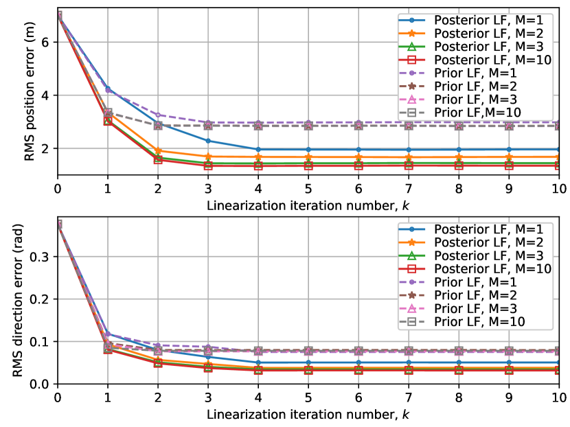
In order to examine the performance of Algorithm 1, in Fig. 4 we plot the RMS position and direction error against the number of linearization iteration $K$. Notice the performance gap between the prior linearization filter (LF) (dotted lines) and the posterior LF (solid lines). After each belief propagation iteration, the posterior of each vehicle is closer to the true state than the prior, so the belief propagation has a better performance on the posterior linearization measurement model. Both position RMSE and direction RMSE converged for linearization iteration number larger than 4. Meanwhile, increasing $M$ from 1 to 3 provides significant improvements for both position and orientation estimation accuracy as the beliefs are more accurate. The improvement becomes very small for $M$ greater than 3.

IV-B2 Localization Performance

Figure 5: CDF of localization and orientation error, $K=10$.

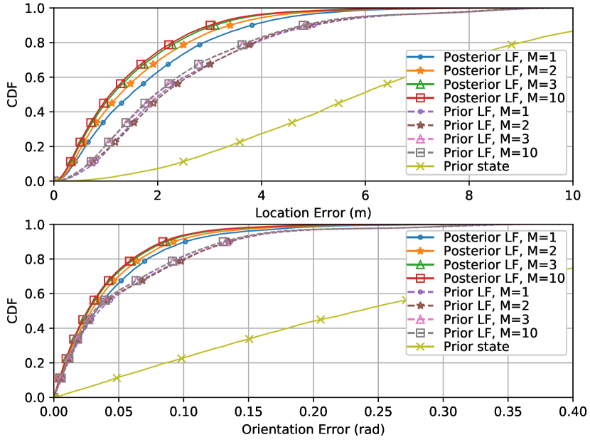
While the above results show the average RMSE of the position and direction, Fig. 5 shows the cumulative distribution functions (CDFs) of the position and direction errors for $K=10$ for different values of $M$. We observe that for $M=3$ the performance is similar to $M=10$ and that nearly all vehicles can be localized with a position error less then 4 meters and an orientation error less than 0.15 radians (8 degrees). The importance of posterior linearization over prior linearization is again clear.

IV-B3 Impact of Network parameters

Figure 6: The impact of 4 vehicle network parameters on localization and orientation performance. Lines with square and triangle markers represent the position and orientation RMSE, respectively. $K=10$, $M=10$ and posterior LF are applied.

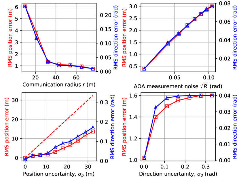
Here, we analyze the impact of modifying the scenario parameters in Table I on localization and orientation estimation performance. In Fig. 6, we evaluate 4 parameters separately, namely communication radius ($r$), measurement noise variance ($R$), prior uncertainty in position ($\sigma_{p}=(\sigma_{x}^{2}+\sigma_{y}^{2})^{1/2}$) and prior uncertainty in orientation ($\sigma_{\theta}$) in 4 sub-figures, by plotting the position and direction RMSE as functions of one of them, while keeping the rest fixed to the values of Table I.

• The top left sub-figure shows the impact of the communication radius $r$. Both RMSEs are reduced rapidly by increasing $r$ from 10 m to 30 m since each vehicle has more neighbors and the network connectivity increases quickly, up to the point where all vehicles are in each others’ communication range. We note that with increased connectivity comes increased computational complexity.

• In the top right sub-figure, we vary the AoA measurements noise variance $R$. We note that both direction and position RMSE increase approximately linearly in $\sqrt{R}$. This emphasizes the need for good measurements.

• The influence of the prior position uncertainty ($\sqrt{\sigma_{x},\sigma_{y}}$) is shown in the bottom left sub-figure. The red dashed line describes the prior position RMSE. We notice the increase of $\sigma_{p}$ from 0 m to 10 m has small effect on both position and direction performance (less than 2 m/0.05 rad), showing the good performance of the proposed method. For position uncertainty over 10 m, Algorithm 1 is still able to improve performance over the prior RMSE, but leads to progressively larger errors. This is in contrast to range-based cooperative localization [2], where no prior information was needed.

• The influence of the direction uncertainty ($\sigma_{\theta}$) is shown in the bottom right sub-figure, where we observe a rapid increase in RMSE. This is because the AoA measurements depend on the orientation of the receiving vehicles. For larger prior orientation uncertainty, Algorithm 1 is less affected.

V Conclusion

We have applied PLBP to cooperative localization (position and orientation estimation) of vehicles with AoA-only measurements. Multiple conditions of the vehicular network, including the vehicle density, communication radius, prior uncertainty and measurement noise variance have been discussed. Numerical results show that the proposed algorithm has good performance in terms of both position and orientation estimation, and only a few iterations are required for convergence. This makes the algorithm attractive for real-time processing.

Appendix A Steps of the posterior linearization

This section illustrates the procedures of SLR on the measurement model and the approximation of the parameters ($\mathbf{C}_{ij},\mathbf{\Omega}_{i,j}$) with respect to the joint posterior PDF $p(\mathbf{x}_{ij}|\mathbf{z}_{ij})$ = $\mathcal{N}(\mathbf{x}_{ij};\bm{\mu}_{ij};\mathbf{P}_{ij})$. First, according to the joint posterior of $\mathbf{x}_{i},\mathbf{x}_{j}$, we select $L$ sigma-points $\mathcal{X}_{1},...,\mathcal{X}_{L}$ and weights $\omega_{1},...,\omega_{L}$ using a sigma-point method such as the unscented transform [26]. Then we calculate the transformed sigma points by

$$\mathcal{Z}_{l}=\mathbf{h}_{ij}(\mathcal{X}_{l})\hskip 10.0ptl=1,...,L$$ (14)

However, as mentioned in Section II, the function arctan has discontinuity problem at the negative $x$ semi-axis. The sigma points transformation needs an ad-hoc modification so that the difference between angles $\mathcal{Z}_{l}-\mathbf{z}_{ij}$ must be bounded in $\pm\pi$. $\mathcal{Z}_{l}$ can be corrected to $\hat{\mathcal{Z}_{l}}$ by the following transformation:

$$\hat{\mathcal{Z}_{l}}=\mathbf{z}_{ij}+\pi-\text{modulo}((\mathbf{z}_{ij}-\mathcal{Z}_{l})+\pi)_{2\pi}$$ (15)

where $\hat{\mathcal{Z}_{l}}$ denotes the corrected sigma point, $z_{ij}$ is the AoA measurements and $\text{modulo}(\cdot)_{2\pi}$ represents the modulo operation.

Introducing $\mathbf{C}_{ij}=[\mathbf{A}_{ij}~{}\mathbf{b}_{ij}]$, so that

$$\mathbf{h}_{ij}(\mathbf{x}_{ij}) \approx\mathbf{A}_{ij}\mathbf{x}_{ij}+\mathbf{b}_{ij}+\mathbf{e}_{ij},$$ (16)

the solution of the approximation of $\mathbf{A}_{ij},\mathbf{b}_{ij},\Omega_{i,j}$ is

$$\mathbf{A}_{ij} =\mathbf{C}_{xz}^{\mathsf{T}}\mathbf{P}_{ij}^{-1}$$ (17)

$$\mathbf{b}_{ij} =\bar{z}-\mathbf{A}_{ij}\bm{\mu}_{ij}$$ (18)

$$\mathbf{\Omega}_{i,j} =\mathbf{C}_{zz}-\mathbf{A}_{ij}\mathbf{P}_{ij}\mathbf{A}_{ij}^{\mathsf{T}}$$ (19)

where $\bar{z}$, $\mathbf{C}_{xz}$ and $\mathbf{C}_{zz}$ are approximated using the sigma-points (15) and weights by

$$\bar{z}\approx \sum_{j=1}^{L}\omega_{j}\hat{\mathcal{Z}_{l}}$$ (20)

$$\mathbf{C}_{xz}\approx \sum_{j=1}^{L}\omega_{j}(\mathcal{X}_{j}-\bm{\mu}_{ij})(\hat{\mathcal{Z}_{l}}-\bar{z})^{\mathsf{T}}$$ (21)

$$\mathbf{C}_{zz}\approx \sum_{j=1}^{L}\omega_{j}(\hat{\mathcal{Z}_{l}}-\bar{z})(\hat{\mathcal{Z}_{l}}-\bar{z})^{\mathsf{T}}.$$ (22)

Appendix B Implementation of BP in the linearized model

This section illustrates the derivation of equation (8)–(9) and (10). Once we have the approximated linearization model 11, we can represent the BP message $m^{(k)}_{i\rightarrow j}$ by the Gaussian format [20]

$$m^{(k)}_{i\to j}(\mathbf{x}_{j})\propto\mathcal{N}(\bm{\alpha}^{(k)}_{ij};\mathbf{H}^{(k)}_{ij}\mathbf{x}_{j},\bm{\Gamma}^{(k)}_{ij})$$ (23)

where $\bm{\alpha}^{(k)}_{ij}$, $\mathbf{H}^{(k)}_{ij}$ and $\bm{\Gamma}^{(k)}_{ij}$ are

$$\bm{\alpha}^{(k)}_{ij}=[\mathbf{z}_{ij}]_{1}-\mathbf{A}_{i}\bm{\mu}^{(k-1)}_{ij}-b_{ij}$$ (24a)

$$\mathbf{H}^{(k)}_{ij}=\mathbf{A}_{j}$$ (24b)

$$\bm{\Gamma}^{(k)}_{ij}=\mathbf{R}_{ij}+\bm{\Omega}_{ij}+\mathbf{A}_{i}\mathbf{P}^{(k-1)}_{ij}\mathbf{A}_{i}^{\intercal}$$ (24c)

where $[\mathbf{z}_{ij}]_{1}$ is the AoA measurement received by vehicle $i$, $\mathbf{A}_{i},\mathbf{A}_{j}$ are defined at Section III-B and $\bm{\mu}^{(k-1)}_{ij}$ and $\mathbf{P}^{(k-1)}_{ij}$ are found from the relation

$$\begin{split}\mathcal{N}(\bm{\mu}^{(k-1)}_{ij},\mathbf{P}^{(k-1)}_{ij})\propto\mathcal{N}(\mathbf{x}_{i};\bm{\mu}_{i},\mathbf{P}_{i})\prod_{j^{\prime}\in\mathcal{N}_{i}\backslash j}m^{(k-1)}_{j^{\prime}\rightarrow i}(\mathbf{x}_{i})\end{split}$$ (25)

where the Kalman update step [20, Algorithm 1] is performed to update each message $m^{(k-1)}_{j^{\prime}\to i}(\mathbf{x}_{i})$ on the prior state $\mathcal{N}(\mathbf{x}_{i};\bm{\mu}_{i},\mathbf{P}_{i})$.

To get the local belief (8) at the $k$-th iteration, we can also use Kalman filter update step to update the vehicle prior with all its incoming messages.

$$b_{j}^{(k)}(\mathbf{x}_{j})=\mathcal{N}(\mathbf{x}_{j};\bm{\mu}_{j},\mathbf{P}_{j})\times\prod_{i\in\mathcal{N}_{j}}m^{(k)}_{i\to j}(\mathbf{x}_{j})$$ (26)

The $k$-th iteration joint posterior (10) is expressed as [20]

$$b^{(k)}(\mathbf{x}_{ij})=\mathcal{N}(\mathbf{x}_{i};\bm{\mu}_{i},\mathbf{P}_{i})\prod_{j^{\prime}\in\mathcal{N}_{i}\backslash j}m^{(k)}_{j^{\prime}\to i}(\mathbf{x}_{i})$$ (27)

$$\times\mathcal{N}(\mathbf{x}_{j},\bm{\mu}_{j},\mathbf{P}_{j})\times\prod_{i^{\prime}\in\mathcal{N}_{j}\backslash i}m^{(k)}_{i^{\prime}\rightarrow j}(\mathbf{x}_{j})p(\mathbf{z}_{ij}|\mathbf{x}_{i},\mathbf{x}_{j})$$

where we can also apply Kalman filter update [20, Algorithm 1] as in (25).

References

- [1] S. Gleason, D. Gebre-Egziabher, and D. G. Egziabher, “GNSS applications and methods,” 2009.
- [2] H. Wymeersch, J. Lien, and M. Z. Win, “Cooperative localization in wireless networks,” Proceedings of the IEEE, vol. 97, no. 2, pp. 427–450, Mar. 2009.
- [3] F. de Ponte Müller, “Survey on ranging sensors and cooperative techniques for relative positioning of vehicles,” Sensors, vol. 17, no. 2, p. 271, Jan. 2017.
- [4] F. R. Kschischang, B. J. Frey, H.-A. Loeliger et al., “Factor graphs and the sum-product algorithm,” IEEE Transactions on information theory, vol. 47, no. 2, pp. 498–519, Jul. 2001.
- [5] E. Steinmetz, R. Emardson, F. Brännström, and H. Wymeersch, “Theoretical limits on cooperative positioning in mixed traffic,” IEEE Access, vol. 7, pp. 49 712–49 725, 2019.
- [6] P. H. Mohammadabadi and S. Valaee, “Cooperative node positioning in vehicular networks using inter-node distance measurements,” in 2014 IEEE 25th Annual International Symposium on Personal, Indoor, and Mobile Radio Communication (PIMRC). IEEE, 2014, pp. 1448–1452.
- [7] A. Catovic and Z. Sahinoglu, “The Cramer-Rao bounds of hybrid TOA/RSS and TDOA/RSS location estimation schemes,” IEEE Communications Letters, vol. 8, no. 10, pp. 626–628, Jan. 2004.
- [8] M. R. Gholami, S. Gezici, E. G. Strom, and M. Rydstrom, “Hybrid TW-TOA/TDOA positioning algorithms for cooperative wireless networks,” in 2011 IEEE International Conference on Communications (ICC). IEEE, Jul. 2011, pp. 1–5.
- [9] R. M. Buehrer, H. Wymeersch, and R. M. Vaghefi, “Collaborative sensor network localization: Algorithms and practical issues,” Proceedings of the IEEE, vol. 106, no. 6, pp. 1089–1114, Jun. 2018.
- [10] N. Alam and A. G. Dempster, “Cooperative positioning for vehicular networks: Facts and future,” IEEE transactions on intelligent transportation systems, vol. 14, no. 4, pp. 1708–1717, Jun. 2013.
- [11] S. Sakagami, S. Aoyama, K. Kuboi, S. Shirota, and A. Akeyama, “Vehicle position estimates by multibeam antennas in multipath environments,” IEEE Transactions on Vehicular Technology, vol. 41, no. 1, pp. 63–68, Feb. 1992.
- [12] A. Fascista, G. Ciccarese, A. Coluccia, and G. Ricci, “Angle of arrival-based cooperative positioning for smart vehicles,” IEEE Transactions on Intelligent Transportation Systems, no. 99, pp. 1–13, Nov. 2017.
- [13] A. Kakkavas, M. H. C. Garcia, R. A. Stirling-Gallacher, and J. A. Nossek, “Multi-array 5G V2V relative positioning: Performance bounds,” in 2018 IEEE Global Communications Conference (GLOBECOM). IEEE, Dec. 2018, pp. 206–212.
- [14] A. F. Garcia-Fernandez, F. Tronarp, and S. Sarkka, “Gaussian target tracking with direction-of-arrival von Mises-Fisher measurements,” IEEE Transactions on Signal Processing, Apr. 2019.
- [15] B. Etzlinger, F. Meyer, A. Springer, F. Hlawatsch, and H. Wymeersch, “Cooperative simultaneous localization and synchronization: A distributed hybrid message passing algorithm,” in Signals, Systems and Computers, 2013 Asilomar Conference on. IEEE, Nov. 2013, pp. 1978–1982.
- [16] V. Savic and S. Zazo, “Cooperative localization in mobile networks using nonparametric variants of belief propagation,” Ad Hoc Networks, vol. 11, no. 1, pp. 138–150, Mar. 2013.
- [17] E. A. Wan and R. Van Der Merwe, “The unscented Kalman filter for nonlinear estimation,” in Proceedings of the IEEE 2000 Adaptive Systems for Signal Processing, Communications, and Control Symposium (Cat. No. 00EX373). IEEE, Oct. 2000, pp. 153–158.
- [18] Á. F. García-Fernández, L. Svensson, M. R. Morelande, and S. Särkkä, “Posterior linearization filter: Principles and implementation using sigma points,” IEEE Transactions on Signal Processing, vol. 63, no. 20, pp. 5561–5573, Jul. 2015.
- [19] W. Yuan, N. Wu, B. Etzlinger, H. Wang, and J. Kuang, “Cooperative joint localization and clock synchronization based on Gaussian message passing in asynchronous wireless networks.” IEEE Trans. Vehicular Technology, vol. 65, no. 9, pp. 7258–7273, Jan. 2016.
- [20] Á. F. García-Fernández, L. Svensson, and S. Särkkä, “Cooperative localization using posterior linearization belief propagation,” IEEE Transactions on Vehicular Technology, vol. 67, no. 1, pp. 832–836, Jan. 2018.
- [21] Y. Shen and M. Z. Win, “On the accuracy of localization systems using wideband antenna arrays,” IEEE Transactions on Communications, vol. 58, no. 1, pp. 270–280, Jan. 2010.
- [22] D. F. Crouse, “Cubature/unscented/sigma point Kalman filtering with angular measurement models,” in 2015 18th International Conference on Information Fusion (Fusion). IEEE, Jul. 2015, pp. 1550–1557.
- [23] Stamen-Map, “Map of central Manhattan,” http://maps.stamen.com/m2i/#toner/256:256/18/40.71590/-73.99560, May. 13, 2019, [May. 27, 2019].
- [24] ——, “Convergence map of the vehicular network scenario,” https://hhsly.github.io/paper_plbp_fig3/, May. 13, 2019, [May. 27, 2019].
- [25] ——, “Initialization map of the vehicular network scenario,” https://hhsly.github.io/paper_plbp_fig2/, May. 13, 2019, [May. 27, 2019].
- [26] S. J. Julier and J. K. Uhlmann, “Unscented filtering and nonlinear estimation,” Proceedings of the IEEE, vol. 92, no. 3, pp. 401–422, 2004.