Assessing Transferability from Simulation to Reality for Reinforcement Learning

Abstract

Learning robot control policies from physics simulations is of great interest to the robotics community as it may render the learning process faster, cheaper, and safer by alleviating the need for expensive real-world experiments. However, the direct transfer of learned behavior from simulation to reality is a major challenge. Optimizing a policy on a slightly faulty simulator can easily lead to the maximization of the ‘Simulation Optimization Bias’ (SOB). In this case, the optimizer exploits modeling errors of the simulator such that the resulting behavior can potentially damage the robot. We tackle this challenge by applying domain randomization, i.e., randomizing the parameters of the physics simulations during learning. We propose an algorithm called Simulation-based Policy Optimization with Transferability Assessment (SPOTA) which uses an estimator of the SOB to formulate a stopping criterion for training. The introduced estimator quantifies the over-fitting to the set of domains experienced while training. Our experimental results on two different second order nonlinear systems show that the new simulation-based policy search algorithm is able to learn a control policy exclusively from a randomized simulator, which can be applied directly to real systems without any additional training.

1 Introduction

Exploration-based learning of control policies on physical systems is expensive in two ways. For one thing, real-world experiments are time-consuming and need to be executed by experts. Additionally, these experiments require expensive equipment which is subject to wear and tear. In comparison, training in simulation provides the possibility to speed up the process and save resources. A major drawback of robot learning from simulations is that a simulation-based learning algorithm is free to exploit any infeasibility during training and will utilize the flawed physics model if it yields an improvement during simulation. This exploitation capability can lead to policies that damage the robot when later deployed in the real world. The described problem is exemplary of the difficulties that occur when transferring robot control policies from simulation to reality, which have been the subject of study for the last two decades under the term ‘reality gap’. Early approaches in robotics suggest using minimal simulation models and adding artificial i.i.d. noise to the system’s sensors and actuators while training in simulation [1]. The aim was to prevent the learner from focusing on small details, which would lead to policies with only marginal applicability. This over-fitting can be described by the Simulation Optimization Bias (SOB), which is similar to the bias of an estimator. The SOB is closely related to the Optimality Gap (OG), which has been used by the optimization community since the 1990s [2, 3], but has not been transferred to robotics or Reinforcement Learning (RL), yet.

Figure 1: Evaluation platforms by Quanser [4]: (left) the 2 DoF Ball-Balancer, (right) the linear inverted pendulum, called Cart-Pole. Both systems are under-actuated nonlinear balancing problems with continuous state and action spaces.

Deep RL algorithms recently demonstrated super-human performance in playing games [5, 6] and promising results in (simulated) robotic control tasks [7, 8, 9]. However, when transferred to real-world robotic systems, most of these methods become less attractive due to high sample complexity and a lack of explainability of state-of-the-art deep RL algorithms. As a consequence, the research field of domain randomization has recently been gaining interest [10, 11, 12, 13, 14, 15, 16, 17]. This class of approaches promises to transfer control policies learned in simulation (source domain) to the real world (target domain) by randomizing the simulator’s parameters (e.g., masses, extents, or friction coefficients) and hence train from a set of models instead of just one nominal model. Further motivation to investigate domain randomization is given by the recent successes in robotic sim-to-real scenarios, such as the in-hand manipulation of a cube [18], swinging a peg in a hole, or opening a drawer [17]. The idea of randomizing the simulator’s parameters is driven by the fact that the corresponding true parameters of the target domain are unknown. However, instead of relying on an accurate estimation of one fixed parameter set, we take a Bayesian point of view and assume that each parameter is drawn from an unknown underlying distribution. Thereby, the expected effect is an increase in robustness of the learned policy when applied to a different domain. Throughout this paper, we use the term robustness to describe a policy’s ability to maintain its performance under model uncertainties. In that sense, a robust control policy is more likely to overcome the reality gap.

Looking at the bigger picture, model-based control only considers a system’s nominal dynamics parameter values, while robust control minimizes a system’s sensitivity with respect to bounded model uncertainties, thus focuses the worst-case. In contrast to these methods, domain randomization takes the whole range of parameter values into account.

Contributions: we advance the state-of-the-art by

1. introducing a measure for the transferability of a solution, i.e., a control policy, from a set of source distributions to a different target domain from the same distribution,

2. designing an algorithm which, based on this measure, is able to transfer control policies from simulation to reality without any real-world data, and

3. validating the approach by conducting two sim-to-real experiments on under-actuated nonlinear systems.

The remainder of this paper is organized as follows: we explain the necessary fundamentals (Section 2) for the proposed algorithm (Section 3). In particular, we derive the Simulation Optimization Bias (SOB) and the Optimality Gap (OG). After validating the proposed method in simulation, we evaluate it experimentally (Section 4). Next, the connection to related work is discussed (Section 5). Finally, we conclude and discuss possible future research directions (Section 6).

2 Problem Statement and Notation

Optimizing policies for Markov Decision Processes with unknown dynamics is generally a hard problem (Section 2.1). Specifically, this problem is hard due to the simulation optimization bias (Section 2.2), which is related to the optimality gap (Section 2.3). We derive an upper bound on the optimality gap, show its monotonic decrease with increasing number of samples from the random variable. Moreover, we clarify the relationship between the simulation optimization bias and the optimality gap (Section 2.4). In what follows, we build upon the results of [2, 3].

2.1 Markov Decision Process

Consider a time-discrete dynamical system

$$\begin{gathered}\fs_{t+1}\sim\mathcal{P}_{\fxi}\left(\left.\fs_{t+1}\right|\fs_{t},\fa_{t},\fxi\right),\quad\fs_{0}\sim\mu_{0,\fxi}(\left.\fs_{0}\right|\fxi),\\ \fa_{t}\sim\pi\!\left(\left.\fa_{t}\right|\fs_{t};\ftheta\right),\quad\fxi\sim\nu\!\left(\fxi;\fphi\right),\end{gathered}$$ (1)

with the continuous state ${\fs_{t}\in\mathcal{S}_{\fxi}\subseteq\mathbb{R}^{{n_{s}}}}$, and continuous action ${\fa_{t}\in\mathcal{A}_{\fxi}\subseteq\mathbb{R}^{{n_{a}}}}$ at time step $t$. The environment, also called domain, is instantiated through its parameters ${\fxi\in\mathbb{R}^{{n_{\xi}}}}$ (e.g., masses, friction coefficients, or time delays), which are assumed to be random variables distributed according to the probability distribution ${\nu\colon\mathbb{R}^{{n_{\xi}}}\to\mathbb{R}^{+}}$ parametrized by $\fphi$. These parameters determine the transition probability density function ${\mathcal{P}_{\fxi}\colon\mathcal{S}_{\fxi}\times\mathcal{A}_{\fxi}\times\mathcal{S}_{\fxi}\to\mathbb{R}^{+}}$ that describes the system’s stochastic dynamics. The initial state $\fs_{0}$ is drawn from the start state distribution ${\mu_{0,\fxi}\colon\mathcal{S}_{\fxi}\to\mathbb{R}^{+}}$. Together with the reward function ${r\colon\mathcal{S}_{\fxi}\times\mathcal{A}_{\fxi}\to\mathbb{R}}$, and the temporal discount factor ${\gamma\in[0,1]}$, the system forms a MDP described by the tuple ${\mathcal{M}_{\fxi}=\left\langle\mathcal{S}_{\fxi},\mathcal{A}_{\fxi},\mathcal{P}_{\fxi},\mu_{0,\fxi},r,\gamma\right\rangle}$.

The goal of a Reinforcement Learning (RL) agent is to maximize the expected (discounted) return, a numeric scoring function which measures the policy’s performance. The expected discounted return of a stochastic domain-independent policy $\pi\!\left(\left.\fa_{t}\right|\fs_{t};\ftheta\right)$, characterized by its parameters $\ftheta\in\Theta\subseteq\mathbb{R}^{{n_{\theta}}}$, is defined as

$$J\!\left(\ftheta,\fxi,\fs_{0}\right)=\mathbb{E}_{\ftau}\!\left[\sum_{t=0}^{T-1}\gamma^{t}r(\fs_{t},\fa_{t})\Bigg{|}\ftheta,\fxi,\fs_{0}\right].$$ (2)

While learning from trial and error, the agent adapts its policy parameters. The resulting state-action-reward tuples are collected in trajectories, a.k.a. rollouts, $\ftau=\{\fs_{t},\fa_{t},r_{t}\}_{t=0}^{T-1}$, with ${r_{t}=r(\fs_{t},\fa_{t})}$. To keep the notation concise, we omit the dependency on the initial state $\fs_{0}$.

2.2 Simulation Optimization Bias (SOB)

Figure 2: Simulation Optimization Bias (SOB) between the true optimum $\theta^{\star}$ and the sample-based optimum $\theta_{n}^{\star}$. The shaded region visualizes the standard deviation around $J\!\left(\theta\right)$, and $\hat{J}_{n}\!\left(\theta\right)$ is determined by a particular set of $n$ sampled domain parameters.

Table I: Definition and of the expectation of the expected (discounted) return, the Simulation Optimization Bias (SOB), the Optimality Gap (OG), and its estimation. All approximations are based on $n$ domains.

Name	Definition	Property
estimated expectation of the expected return	$\hat{J}_{n}\!\left(\ftheta\right)=\frac{1}{n}\sum_{i=1}^{n}J\!\left(\ftheta,\fxi_{i}\right)$	$\mathbb{E}_{\fxi}\!\left[\hat{J}_{n}\!\left(\ftheta\right)\right]=J\!\left(\ftheta\right)$
simulation optimization bias	$\mathrm{b}\!\left[\hat{J}_{n}\!\left(\ftheta_{n}^{\star}\right)\right]=\mathbb{E}_{\fxi}\!\Big{[}\max_{\hat{\ftheta}\in\Theta}\hat{J}_{n}(\hat{\ftheta})\Big{]}-\max_{\ftheta\in\Theta}\mathbb{E}_{\fxi}\!\Big{[}J\!\left(\ftheta,\fxi\right)\Big{]}$	$\mathrm{b}\!\left[\hat{J}_{n}\!\left(\ftheta_{n}^{\star}\right)\right]\geq 0$
optimality gap at solution $\ftheta^{c}$	$G\!\left(\ftheta^{c}\right)=\max_{\ftheta\in\Theta}\mathbb{E}_{\fxi}\!\left[J\!\left(\ftheta,\fxi\right)\right]-\mathbb{E}_{\fxi}\!\left[J\!\left(\ftheta^{c},\fxi\right)\right]$	$G\!\left(\ftheta^{c}\right)\geq 0$
estimated optimality gap at solution $\ftheta^{c}$	$\hat{G}_{n}\!\left(\ftheta^{c}\right)=\max_{\ftheta\in\Theta}\hat{J}_{n}\!\left(\ftheta\right)-\hat{J}_{n}\!\left(\ftheta^{c}\right)$	$\hat{G}_{n}\!\left(\ftheta^{c}\right)\geq G\!\left(\ftheta^{c}\right)$

Augmenting the standard RL setting with the concept of domain randomization, i.e. maximizing the expectation of the expected return over all (feasible) realizations of the source domain, leads to the score

$$J\!\left(\ftheta\right)=\mathbb{E}_{\fxi}\!\left[J\!\left(\ftheta,\fxi\right)\right]$$ (3)

that quantifies how well the policy is expected to perform over an infinite set of variations of the nominal domain $\mathcal{M}_{\bar{\fxi}}$. When training exclusively in simulation, the true physics model is unknown and the true $J\!\left(\ftheta,\fxi\right)$ is thus inaccessible. Instead, we maximize the estimated expected return using a randomized physics simulator. Thereby, we update the policy parameters $\ftheta$ with a policy optimization algorithm based on samples. The inevitable imperfections of physics simulations will automatically be exploited by any optimization method to achieve a ‘virtual’ improvement, i.e., an increase of $J\!\left(\ftheta\right)$, in simulation. To formulate this undesirable behavior, we frame the standard RL problem as a Stochastic Program (SP)

$$J\!\left(\ftheta^{\star}\right)=\max_{\ftheta\in\Theta}\mathbb{E}_{\fxi}\!\left[J\!\left(\ftheta,\fxi\right)\right]=\max_{\ftheta\in\Theta}J\!\left(\ftheta\right),$$ (4)

with the optimal solution $\ftheta^{\star}=\operatorname*{arg\,max}_{\ftheta\in\Theta}J\!\left(\ftheta\right)$.

The SP above can be approximated using $n$ domains

$$\hat{J}_{n}\!\left(\ftheta_{n}^{\star}\right)=\max_{\ftheta\in\Theta}\hat{J}_{n}\!\left(\ftheta\right)=\max_{\ftheta\in\Theta}\frac{1}{n}\sum_{i=1}^{n}J\!\left(\ftheta,\fxi_{i}\right),$$ (5)

where the expectation is replaced by the Monte-Carlo estimator over the samples $\fxi_{1},\dots,\fxi_{n}$, and ${\ftheta_{n}^{\star}=\operatorname*{arg\,max}_{\ftheta\in\Theta}\hat{J}_{n}\!\left(\ftheta\right)}$ is the solution to the approximated SP. Note that the expectations in (4, 5) both jointly depend on $\fxi$ and $\fs_{0}$, i.e. both random varaibles are integrated out, but the dependency on $\fs_{0}$ is omitted as stated before.

Sample-based optimization is guaranteed to be optimistically biased if there are errors in the domain parameter estimate, even if these errors are unbiased [2]. Since the proposed method randomizes the domain parameters $\fxi$, this assumption is guaranteed to hold. Using Jensen’s inequality, we can show that the Simulation Optimization Bias (SOB)

$$\mathrm{b}\!\left[\hat{J}_{n}\!\left(\ftheta_{n}^{\star}\right)\right]=\underbrace{\mathbb{E}_{\fxi}\!\Big{[}\max_{\hat{\ftheta}\in\Theta}\hat{J}_{n}(\hat{\ftheta})\Big{]}}_{\text{sample optimum}}-\underbrace{\max_{\ftheta\in\Theta}\mathbb{E}_{\fxi}\!\Big{[}J\!\left(\ftheta,\fxi\right)\Big{]}}_{\text{true optimum}}\geq 0.$$ (6)

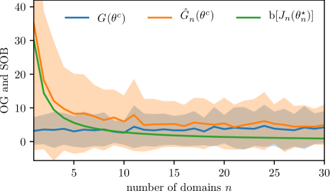
is always positive, i.e. the policy’s performance in the target domain is systematically overestimated. A visualization of the SOB is depicted in Figure 2.

2.3 Optimality Gap (OG)

Intuitively, we want to minimize the SOB in order to achieve the highest transferability of the policy. Since computing the SOB (6) is intractable, the approach presented in this paper is to approximate the Optimality Gap (OG), which relates to the SOB as explained in the Section 2.4.

The OG at the solution candidate $\ftheta^{c}$ is defined as

$$G\!\left(\ftheta^{c}\right)=J\!\left(\ftheta^{\star}\right)-J\!\left(\ftheta^{c}\right)\geq 0,$$ (7)

where ${J\!\left(\ftheta^{\star}\right)=\max_{\ftheta\in\Theta}\mathbb{E}_{\fxi}\!\left[J\!\left(\ftheta,\fxi\right)\right]}$ is the SP’s optimal objective function value and ${J\!\left(\ftheta^{c}\right)=\mathbb{E}_{\fxi}\!\left[J\!\left(\ftheta^{c},\fxi\right)\right]}$ is the SP’s objective function evaluated at the candidate solution [3]. Thus, $G\!\left(\ftheta^{c}\right)$ expresses the difference in performance between the optimal policy and the candidate solution at hand. Unfortunately, computing the expectation over infinitely many domains in (7) is intractable. However, we can estimate $G\!\left(\ftheta^{c}\right)$ from samples.

2.3.1 Estimation of the Optimality Gap

For an unbiased estimator $\hat{J}_{n}\!\left(\ftheta\right)$, e.g. a sample average with i.i.d. samples, he have

$$\mathbb{E}_{\fxi}\!\big{[}\hat{J}_{n}\!\left(\ftheta\right)\big{]}=\mathbb{E}_{\fxi}\!\left[J\!\left(\ftheta,\fxi\right)\right]=J\!\left(\ftheta\right).$$ (8)

Inserting (8) into the first term of (7) yields

$$G\!\left(\ftheta^{c}\right) =\max_{\ftheta\in\Theta}\mathbb{E}_{\fxi}\!\left[\hat{J}_{n}\!\left(\ftheta\right)\right]-\mathbb{E}_{\fxi}\!\left[J\!\left(\ftheta^{c},\fxi\right)\right]$$ (9)

$$\leq\mathbb{E}_{\fxi}\!\left[\max_{\ftheta\in\Theta}\hat{J}_{n}\!\left(\ftheta\right)\right]-\mathbb{E}_{\fxi}\!\left[J\!\left(\ftheta^{c},\fxi\right)\right]$$ (10)

as an upper bound on the OG. To compute this upper bound, we use the law of large numbers for the first term and replace the second expectation in (10) with the sample average

$$G\!\left(\ftheta^{c}\right)\leq\max_{\ftheta\in\Theta}\hat{J}_{n}\!\left(\ftheta\right)-\hat{J}_{n}\!\left(\ftheta^{c}\right)=\hat{G}_{n}\!\left(\ftheta^{c}\right),$$ (11)

where $\hat{G}_{n}\!\left(\ftheta^{c}\right)\geq 0$ holds. Averaging over a finite set of domains allows for the utilization of an estimated upper bound of the OG as the convergence criterion for the policy search meta-algorithm introduced in Section 3.

2.3.2 Decrease of the Estimated Optimality Gap

The OG decreases in expectation with increasing sample size of the domain parameters $\fxi$. The expectation over $\fxi$ of the minuend in (11) estimated from $n+1$ i.i.d. samples is

$$\mathbb{E}_{\fxi}\!\left[\hat{J}_{n+1}\!\left(\ftheta_{n+1}^{\star}\right)\right] =\mathbb{E}_{\fxi}\!\left[\max_{\ftheta\in\Theta}\frac{1}{n+1}\sum\limits_{i=1}^{n+1}J\!\left(\ftheta,\fxi_{i}\right)\right]$$ (12)

$$=\mathbb{E}_{\fxi}\!\left[\max_{\ftheta\in\Theta}\frac{1}{n+1}\sum\limits_{i=1}^{n+1}\frac{1}{n}\sum\limits_{j=1,j\neq i}^{n+1}J\!\left(\ftheta,\fxi_{j}\right)\right]$$ (13)

$$\leq\mathbb{E}_{\fxi}\!\left[\frac{1}{n+1}\sum\limits_{i=1}^{n+1}\max_{\ftheta\in\Theta}\frac{1}{n}\sum\limits_{j=1,j\neq i}^{n+1}J\!\left(\ftheta,\fxi_{j}\right)\right]$$ (14)

$$=\mathbb{E}_{\fxi}\!\left[\hat{J}_{n}\!\left(\ftheta_{n}^{\star}\right)\right].$$ (15)

Taking the expectation of the OG estimated from $n+1$ samples $\hat{G}_{n+1}\!\left(\ftheta^{c}\right)$ and then plugging in the upper bound from (15), we obtain the upper bound

$$\mathbb{E}_{\fxi}\!\left[\hat{G}_{n+1}\!\left(\ftheta^{c}\right)\right] =\mathbb{E}_{\fxi}\!\left[\max_{\ftheta\in\Theta}\hat{J}_{n+1}\!\left(\ftheta\right)-\hat{J}_{n}\!\left(\ftheta^{c}\right)\right]$$ (16)

$$\leq\mathbb{E}_{\fxi}\!\left[\max_{\ftheta\in\Theta}\hat{J}_{n}\!\left(\ftheta\right)-\hat{J}_{n}\!\left(\ftheta^{c}\right)\right]=\mathbb{E}_{\fxi}\!\left[\hat{G}_{n}\!\left(\ftheta^{c}\right)\right],$$ (17)

which shows that the estimator of the OG in expectation monotonically decreases with increasing sample size.

2.4 Connection Between the SOB and the OG

The SOB can be expressed as the expectation of the difference between the approximated OG and the true OG. Starting from the formulation of the approximated OG in (11), we can take the expectation over the domains on both sides of the inequality and rearrange to

$$\mathbb{E}_{\fxi}\!\left[\hat{G}_{n}\!\left(\ftheta^{c}\right)\right]-G\!\left(\ftheta^{c}\right)\geq 0.$$ (18)

Using the definitions of $\hat{G}_{n}\!\left(\ftheta^{c}\right)$ and $G\!\left(\ftheta^{c}\right)$ from Table I, the equation above can be rewritten as

$$\mathbb{E}_{\fxi}\!\left[\max_{\ftheta\in\Theta}\hat{J}_{n}\!\left(\ftheta\right)\right]-\mathbb{E}_{\fxi}\!\left[\hat{J}_{n}\!\left(\ftheta^{c}\right)\right]-$$ (19)

$$\indent\max_{\ftheta\in\Theta}\mathbb{E}_{\fxi}\!\left[J\!\left(\ftheta,\fxi\right)\right]+\mathbb{E}_{\fxi}\!\Big{[}J\!\left(\ftheta^{c},\fxi\right)\Big{]}\geq 0.$$ (20)

Since $\hat{J}_{n}\!\left(\ftheta\right)$ is an unbiased estimator of $J\!\left(\ftheta\right)$, we have

$$\mathbb{E}_{\fxi}\!\left[\hat{J}_{n}\!\left(\ftheta^{c}\right)\right]=\mathbb{E}_{\fxi}\!\left[J\!\left(\ftheta^{c},\fxi\right)\right]=J\!\left(\ftheta^{c}\right).$$ (21)

Hence, the left hand side of (20) becomes

$$\mathbb{E}_{\fxi}\!\left[\max_{\ftheta\in\Theta}\hat{J}_{n}\!\left(\ftheta\right)\right]-\max_{\ftheta\in\Theta}\mathbb{E}_{\fxi}\!\Big{[}J\!\left(\ftheta,\fxi\right)\Big{]}=\mathrm{b}\!\left[\hat{J}_{n}\!\left(\ftheta_{n}^{\star}\right)\right],$$ (22)

which is equal to the SOB defined in (6). Thus, the SOB is the difference between the expectation over all domains of the estimated OG $\hat{G}_{n}\!\left(\ftheta^{c}\right)$ and the true OG $G\!\left(\ftheta^{c}\right)$ at the solution candidate. Therefore, reducing the estimated OG leads to reducing the SOB.

2.5 An Illustrative Example

Imagine we were placed randomly in an environment either on Mars $\fxi_{M}$ or on Venus $\fxi_{V}$, governed by the distribution $\fxi\sim\nu\!\left(\fxi;\phi\right)$. On both planets we are in a catapult about to be shot into the sky exactly vertical. The only thing we can do is to manipulate the catapult, modeled as a linear spring, according to the policy $\pi\!\left(\theta\right)$, i.e. changing the springs extension. Our goal is to minimize the maximum height of the expected flight trajectory $\mathbb{E}_{\fxi}\!\left[h(\theta,\fxi)\right]$ derived from the conservation of energy

$$h(\theta,\fxi_{i})=\frac{k_{i}(\theta-x_{i})^{2}}{2mg_{i}},$$ (23)

with mass $m$, and domain parameters ${\fxi_{i}=\{g_{i},k_{i},x_{i}\}}$ consisting of the gravity acceleration constant, the catapult’s spring stiffness, and the catapult’s spring pre-extension. The domain parameters are the only quantities specific to Mars and Venus. In this simplified example, we assume that the domain parameters are not drawn from individual distributions, but that there are two sets of domain parameters $\fxi_{M}$ and $\fxi_{V}$ which are drawn from a Bernoulli distribution $\mathcal{\mathcal{B}}\left(\fxi\big{|}\phi\right)$ where $\phi$ is the probability of drawing $\fxi_{V}$. Since minimizing $\mathbb{E}_{\fxi}\!\left[h(\theta,\fxi)\right]$ is identical to maximizing its negative value $J\!\left(\theta,\fxi\right)\coloneqq-\mathbb{E}_{\fxi}\!\left[h(\theta,\fxi)\right]$, we rewrite the problem as

$$J\!\left(\theta^{\star}\right)=\max_{\theta\in\Theta}\mathbb{E}_{\fxi}\!\left[J\!\left(\theta,\fxi\right)\right].$$ (24)

Assume we experienced this situation $n$ times and want to find the policy parameter maximizing the objective above without knowing on which planet we are (ı.e., independent of $\fxi$). Thus, we approximate $J\!\left(\theta^{\star}\right)$ by

$$\hat{J}_{n}\!\left(\theta_{n}^{\star}\right)=\max_{\theta\in\Theta}\frac{1}{n}\sum_{i=1}^{n}J\!\left(\theta,\fxi_{i}\right).$$ (25)

In this Bernoulli experiment, the return of a policy $\pi\!\left(\theta\right)$ fully determined by $\theta$ estimates to

$$\hat{J}_{n}\!\left(\theta\right)=\underbrace{\frac{n_{M}}{n}J\!\left(\theta,\fxi_{M}\right)}_{\text{proportion Mars}}+\underbrace{\frac{n_{V}}{n}J\!\left(\theta,\fxi_{V}\right)}_{\text{proportion Venus}}.$$ (26)

The optimal policy given the $n$ domains fulfills the necessary condition

$$0=\nabla_{\theta}\hat{J}_{n}\!\left(\theta_{n}^{\star}\right)=-\frac{n_{M}}{n}\frac{k_{M}(\theta_{n}^{\star}-x_{M})}{mg_{M}}-\frac{n_{V}}{n}\frac{k_{V}(\theta_{n}^{\star}-x_{V})}{mg_{V}}.$$ (27)

Solving for the optimal policy parameter yields

$$\theta_{n}^{\star}=\frac{x_{M}n_{M}k_{M}g_{V}+x_{V}n_{V}k_{V}g_{M}}{n_{M}k_{M}g_{V}+n_{V}k_{V}g_{M}}=\frac{x_{M}c_{M}+x_{V}c_{V}}{c_{M}+c_{V}},$$ (28)

with the (mixed-domain) constants ${c_{M}=n_{M}k_{M}g_{V}}$ and ${c_{V}=n_{V}k_{V}g_{M}}$. Inserting (28) into (26) gives the optimal return value for $n$ samples

$$\hat{J}_{n}\!\left(\theta^{\star}\right) =-\frac{n_{M}k_{M}}{2nmg_{M}}\left(\frac{x_{V}c_{V}-x_{M}c_{V}}{c_{M}+c_{V}}\right)^{2}$$ (29)

$$\qquad-\frac{n_{V}k_{V}}{2nmg_{V}}\left(\frac{x_{M}c_{M}-x_{V}c_{M}}{c_{M}+c_{V}}\right)^{2}.$$ (30)

Given the domain parameters in Table II of Appendix B, we optimize our catapult manipulation policy. This is done in simulation, since real-world trials (being shot with a catapult) would be very costly. Finding the optimal policy in simulation means solving the approximated SP (5), whose optimal solution is denoted by $\theta_{n}^{\star}$. We assume that the (stochastic) optimization algorithm outputs a suboptimal solution $\theta^{c}$. In order to model this property, a policy parameter is sampled in the vicinity of the optimum ${\theta^{c}\sim\mathcal{\mathcal{N}}\left(\theta\big{|}\theta_{n}^{\star};\sigma^{2}_{\theta}\right)}$ with ${\sigma_{\theta}=0.15}$. During the entire process, the true optimal policy parameter $\theta^{\star}$ will remain unknown. However, since this simplified example models the domain parameters to be one of two fixed sets ($\fxi_{M}$ or $\fxi_{V}$), $\theta^{\star}$ can be computed analogously to (28).

Figure 3: The estimated expected return evaluated using the optimal solution for a set of $n$ domains $\hat{J}_{n}\!\left(\theta_{n}^{\star}\right)$, the candidate solution $\hat{J}_{n}\!\left(\theta^{c}\right)$, as well as the true optimal solution $\hat{J}_{n}\!\left(\theta^{\star}\right)$. Note that $\hat{J}_{n}\!\left(\theta_{n}^{\star}\right)>\hat{J}_{n}\!\left(\theta^{c}\right)$ holds for every instance of the 100 random seeds, even if the standard deviation areas overlap. The shaded areas show $\pm 1$ standard deviation.

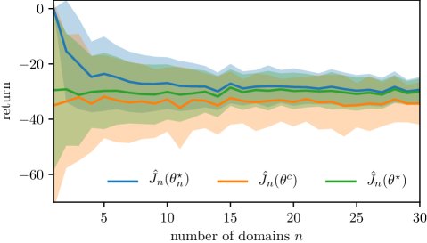
The Figures 3 and 4 visualize the evolution of the approximated SP with increasing number of domains $n$. Key observations are that the objective function value at the candidate solution $\hat{J}_{n}\!\left(\theta^{c}\right)$ is less than at the sample-based optimum $\hat{J}_{n}\!\left(\theta_{n}^{\star}\right)$ (Figure 3), and that with increasing number of domains the SOB $\mathrm{b}[\hat{J}\!\left(\theta_{n}^{\star}\right)]$ decreases monotonically while the estimated OG $\hat{G}_{n}\!\left(\theta^{c}\right)$ only decreases in expectation (Figure 4). When optimizing over $n=30$ random domains in simulation, we yield a policy which leads to a $G_{n}\!\left(\theta^{c}\right)\approx$4.23\text{\,}\mathrm{m}\text{/}$$ higher (worse) shot compared to the best policy computed from an infinite set of domains and evaluated on this infinite set of domains, and a $\hat{G}_{n}\!\left(\theta^{c}\right)\approx$4.97\text{\,}\mathrm{m}\text{/}$$ higher (worse) shot compared to the best policy computed from a set of $n=30$ domains and evaluated on the same finite set of domains. Furthermore, we can say that executing the best policy computed from a set of $n=30$ domains will in reality result in a ${\mathrm{b}[\hat{J}\!\left(\theta_{n}^{\star}\right)]\approx$0.911\text{\,}\mathrm{m}\text{/}$}$ higher (worse) shot.

3 Simulation-Based Policy Optimization with Transferability Assessment

We introduce Simulation-based Policy Optimization with Transferability Assessment (SPOTA) [19], a policy search meta-algorithm which yields a policy that is able to directly transfer from a set of source domains to an unseen target domain. The goal of SPOTA is not only to maximize the expected discounted return under the influence of randomized physics simulations $J\!\left(\ftheta\right)$, but also to provide an approximate probabilistic guarantee on the suboptimality in terms of expected discounted return when applying the obtained policy to a different domain. The key novelty in SPOTA is the utilization of an Upper Confidence Bound on the Optimality Gap (UCBOG) as a stopping criterion for the training procedure of the RL agent.

One interpretation of (source) domain randomization is to see it as a form of uncertainty representation. If a control policy is trained successfully on multiple variations of the scenario, i.e., a set of models, it is legitimate to assume that this policy will be able to handle modeling errors better than policies that have only been trained on the nominal model $\bar{\fxi}=\mathbb{E}_{\nu}\!\left[\fxi\right]$. With this rationale in mind, we propose the SPOTA procedure, summarized in Algorithm 1.

Figure 4: True optimality gap $G\!\left(\theta^{c}\right)$, the approximation from $n$ domains $\hat{G}\!\left(\theta^{c}\right)$, and the simulation optimization bias $\mathrm{b}[\hat{J}_{n}\!\left(\theta_{n}^{\star}\right)]$. Note that $\hat{G}_{n}\!\left(\theta^{c}\right)\geq G\!\left(\theta^{c}\right)$ does not hold for every instance of the 100 random seeds, but is true in expectation. The variance in $G\!\left(\theta^{c}\right)$ is only caused by the variance in $\theta^{c}$. The shaded areas show $\pm 1$ standard deviation.

input : probability distribution $\nu\!\left(\fxi;\fphi\right)$, algorithm PolOpt, sequence NonDecrSeq, hyper-parameters $n_{c}$, ${n_{r}}$, $n_{G}$, $n_{J}$, ${n_{b}}$, $\alpha$, $\beta$

output : policy $\pi\!\left(\ftheta_{{n_{c}}}^{\star}\right)$ with a $(1-\alpha)$-level confidence on $\bar{G}_{{n_{r}}}\!\left(\ftheta_{{n_{c}}}^{\star}\right)$ which is upper bounded by $\beta$

1

2Initialize $\pi\!\left(\ftheta_{n_{c}}\right)$ randomly

3 do

4       Sample ${n_{c}}$ i.i.d. physics simulators described by $\fxi_{1},\dots,\fxi_{{n_{c}}}$ from $\nu\!\left(\fxi;\fphi\right)$

       Solve the approx. SP using $\fxi_{1},\dots,\fxi_{{n_{c}}}$ and PolOpt to obtain $\ftheta_{{n_{c}}}^{\star}$

        $\triangleright$ candidate solution

5       for $k=1,\dots,n_{G}$ do

6             Sample ${n_{r}}$ i.i.d. physics simulators described by $\fxi_{1}^{k},\dots,\fxi_{{n_{r}}}^{k}$ from $\nu\!\left(\fxi;\fphi\right)$

7             Initialize $\ftheta_{{n_{r}}}^{k}$ with $\ftheta_{{n_{c}}}^{\star}$ and reset the exploration strategy

             Solve the approx. SP using $\fxi_{1}^{k},\dots,\fxi_{{n_{r}}}^{k}$ and PolOpt to obtain $\ftheta_{{n_{r}}}^{k\star}$

              $\triangleright$ reference solution

8             for $i=1,\dots,{n_{r}}$ do

9                   with synchronized random seeds $\triangleright$ sync initial states and observation noise

10                         Estimate the candidate solution’s return $\hat{J}_{n_{J}}\!\left(\ftheta_{{n_{c}}}^{\star},\fxi_{i}^{k}\right)\leftarrow 1/n_{J}\sum_{j=1}^{n_{J}}\hat{J}\!\left(\ftheta_{{n_{c}}}^{\star},\fxi_{i}^{k}\right)$

11                         Estimate the $i$-th reference solution’s return $\hat{J}_{n_{J}}\!\left(\ftheta_{{n_{r}}}^{k\star},\fxi_{i}^{k}\right)\leftarrow 1/n_{J}\sum_{j=1}^{n_{J}}\hat{J}\!\left(\ftheta_{{n_{r}}}^{k\star},\fxi_{i}^{k}\right)$

12                   end

13                  

14                   Compute the difference in return $\hat{G}_{{n_{r}},i}^{k}\!\left(\ftheta_{{n_{c}}}^{\star}\right)\leftarrow\hat{J}_{n_{J}}\!\left(\ftheta_{{n_{r}}}^{k\star},\fxi_{i}^{k}\right)-\hat{J}_{n_{J}}\!\left(\ftheta_{{n_{c}}}^{\star},\fxi_{i}^{k}\right)$

15                  

16             end for

17            for $k=1,\dots,n_{G}$ and $i=1,\dots,{n_{r}}$ do $\triangleright$ outlier rejection

18                   if $\hat{G}_{{n_{r}},i}^{k}\!\left(\ftheta_{{n_{c}}}^{\star}\right)<0$ then

19                         for $k^{\prime}=1,\dots,n_{G}$, $k^{\prime}\neq k$ do $\triangleright$ loop over other reference solutions

                               if $\hat{G}_{{n_{r}},i}^{k^{\prime}}\!\left(\ftheta_{{n_{c}}}^{\star}\right)>\hat{G}_{{n_{r}},i}^{k}\!\left(\ftheta_{{n_{c}}}^{\star}\right)$ then $\hat{G}_{{n_{r}},i}^{k}\!\left(\ftheta_{{n_{c}}}^{\star}\right)\leftarrow\hat{G}_{{n_{r}},i}^{k^{\prime}}\!\left(\ftheta_{{n_{c}}}^{\star}\right)$; break

20                                $\triangleright$ replace solution

21                              

22                         end for

23                        

24                   end if

25                  

26             end for

27            

28       end for

      Bootstrap ${n_{b}}$ times from $\mathcal{G}=\{\hat{G}_{{n_{r}},1}^{1}\!\left(\ftheta_{{n_{c}}}^{\star}\right),\dots,\hat{G}_{{n_{r}},{n_{r}}}^{n_{G}}\!\left(\ftheta_{{n_{c}}}^{\star}\right)\}$ to yield $\mathcal{G}_{1}^{B},\dots,\mathcal{G}_{{n_{b}}}^{B}$

        $\triangleright$ bootstrapping

29      

30      Compute the sample mean $\bar{G}_{{n_{r}}}\!\left(\ftheta_{{n_{c}}}^{\star}\right)$ for the original set $\mathcal{G}$

31       Compute the sample means $\bar{G}_{{n_{r}},1}^{B}\!\left(\ftheta_{{n_{c}}}^{\star}\right),\dots,\bar{G}_{{n_{r}},{n_{b}}}^{B}\!\left(\ftheta_{{n_{c}}}^{\star}\right)$ for the sets $\mathcal{G}_{1}^{B},\dots,\mathcal{G}_{{n_{b}}}^{B}$

32      

      Select the $\alpha$-th quantile of the bootstrap samples’ means and obtain the upper bound for the one-sided $(1-\alpha)$-level confidence interval $\bar{G}_{{n_{r}}}^{U}\!\left(\ftheta_{{n_{c}}}^{\star}\right)\leftarrow 2\bar{G}_{{n_{r}}}\!\left(\ftheta_{{n_{c}}}^{\star}\right)-Q_{\alpha}\!\left[\bar{G}_{{n_{r}}}^{B}\!\left(\ftheta_{{n_{c}}}^{\star}\right)\right]$

        $\triangleright$ UCBOG

33      

34      Set the new sample sizes $n_{c}\leftarrow\texttt{NonDecrSeq}(n_{c})$ and ${n_{r}}\leftarrow\texttt{NonDecrSeq}({n_{r}})$

35while $\bar{G}_{{n_{r}}}^{U}\!\left(\ftheta_{{n_{c}}}^{\star}\right)>\beta$

Algorithm 1 Simulation-based Policy Optimization with Transferability Assessment (SPOTA)

SPOTA performs a repetitive comparison of solution candidates against reference solutions in domains that are in the references’ training set but unknown to the candidates. As inputs, we assume a probability distribution over the domain parameters $\nu\!\left(\fxi;\fphi\right)$, a policy optimization sub-routine PolOpt, the number of candidate and reference domains ${n_{c}}$ and ${n_{r}}$ in conjunction with a nondecreasing sequence NonDecrSeq (e.g., $n_{k+1}=2n_{k}$), the number of reference solutions $n_{G}$, the number of rollouts used for each OG estimate $n_{J}$, the number of bootstrap samples ${n_{b}}$, the confidence level (1$-\alpha$) used for bootstrapping, and the threshold of trust $\beta$ determining the stopping condition. SPOTA consists of four blocks: finding a candidate solution, finding multiple reference solutions, comparing the candidate against the reference solutions, and assessing the candidate solution quality.

Candidate Solutions are randomly initialized and optimized based on a set of ${n_{c}}$ source domains (Lines 1–1). Practically, the locally optimal policy parameters are optimized on the approximated SP (5).

Reference Solutions are gathered $n_{G}$ times by solving the same approximated SP as for the candidate but with different realizations of the random variable $\fxi$ (Lines 1–1). These $n_{G}$ non-convex optimization processes all use the same candidate solution $\ftheta_{{n_{c}}}^{\star}$ as initial guess.

Solution Comparison is done by evaluating each reference solution $\ftheta_{{n_{r}}}^{k\star}$ with $k=1,\dots,n_{G}$ against the candidate solution $\ftheta_{{n_{c}}}^{\star}$ for each realization of the random variable $\fxi_{i}^{k}$ with $i=1,\dots,{n_{r}}$ on which the reference solution has been trained. In this step, the performances per domain $\hat{J}_{n_{J}}\!\left(\ftheta_{{n_{c}}}^{\star},\fxi_{i}^{k}\right)$ and $\hat{J}_{n_{J}}\!\left(\ftheta_{{n_{r}}}^{k\star},\fxi_{i}^{k}\right)$ are estimated from $n_{J}$ Monte-Carlo simulations with synchronized random seeds (Lines 1–1). Thereby, both solutions are evaluated using the same random initial states and observation noise. Due to the potential suboptimality of the reference solutions, the resulting difference in performance

$$\hat{G}_{{n_{r}},i}^{k}\!\left(\ftheta_{{n_{c}}}^{\star}\right)=\hat{J}_{n_{J}}\!\left(\ftheta_{{n_{r}}}^{k\star},\fxi_{i}^{k}\right)-\hat{J}_{n_{J}}\!\left(\ftheta_{{n_{c}}}^{\star},\fxi_{i}^{k}\right)$$ (31)

may become negative (Line 1). This issue did not appear in previous work on assessing solution qualities of SP [3, 20], because they only covered convex problems, where all reference solutions are guaranteed to be global optima. Utilizing the definition of the OG in (11) for SPOTA demands for globally optimal reference solutions. Due to the non-convexity of the introduced RL problem the obtained solutions by the optimizer only are locally optimal. In order to alleviate this dilemma, we perform an outlier rejection routine (Lines 1–1). As a first attempt, all other reference solutions are evaluated for the current domain $i$. If a solution with higher performance was found, it replaces the current reference solution $k$ for this domain. If all reference solutions are worse than the candidate, the value is clipped to the theoretical minimum (zero).

Solution Quality is assessed by constructing a (1$-\alpha$)-level confidence interval $\left[0,\bar{G}_{{n_{r}}}^{U}\!\left(\ftheta_{{n_{c}}}^{\star}\right)\right]$ for the estimated OG at $\ftheta_{{n_{c}}}^{\star}$. While the lower bound is fixed to the theoretical minimum, the Upper Confidence Bound on the Optimality Gap (UCBOG) is computed using the statistical bootstrap method [21]. We denote bootstrapped quantities with the superscript $B$ instead of the common asterisk, to avoid a notation conflict with the optimal solutions. There are multiple ways to yield a confidence interval by applying the bootstrap [22]. Here, the ’basic’ nonparametric method was chosen, since the aforementioned potential clipping changes the distribution of the samples and hence a method relying on the estimation of population parameters such as the standard error is inappropriate. The solution comparison yields a set of $n_{G}{n_{r}}$ samples of the approximated OG $\mathcal{G}=\{\hat{G}_{{n_{r}},1}^{1}\!\left(\ftheta_{{n_{c}}}^{\star}\right),\dots,\hat{G}_{{n_{r}},{n_{r}}}^{n_{G}}\!\left(\ftheta_{{n_{c}}}^{\star}\right)\}$. Through uniform random sampling with replacement from $\mathcal{G}$, we generate ${n_{b}}$ bootstrap samples $\mathcal{G}_{1}^{B},\dots,\mathcal{G}_{{n_{b}}}^{B}$. Thus, for our statistic of interest, the mean estimated OG $\bar{G}_{{n_{r}}}\!\left(\ftheta_{{n_{c}}}^{\star}\right)$, the UCBOG becomes

$$\bar{G}_{{n_{r}}}^{U}\!\left(\ftheta_{{n_{c}}}^{\star}\right)=2\bar{G}_{{n_{r}}}\!\left(\ftheta_{{n_{c}}}^{\star}\right)-Q_{\alpha}\!\left[\bar{G}_{{n_{r}}}^{B}\!\left(\ftheta_{{n_{c}}}^{\star}\right)\right],$$ (32)

where $\bar{G}_{{n_{r}}}\!\left(\ftheta_{{n_{c}}}^{\star}\right)$ is the mean over all (nonnegative) samples from the empirical distribution, and $Q_{\alpha}\!\left[\bar{G}_{{n_{r}}}^{B}\!\left(\ftheta_{{n_{c}}}^{\star}\right)\right]$ is the $\alpha$-th quantile of the means calculated for each of the ${n_{b}}$ bootstrap samples (Lines 1–1). Consequently, the true OG is lower than the obtained one-sided confidence interval with the approximate probability of (1$-\alpha$), i.e.,

$$\mathbb{P}\left({G\!\left(\ftheta_{{n_{c}}}^{\star}\right)\leq\bar{G}_{{n_{r}}}^{U}\!\left(\ftheta_{{n_{c}}}^{\star}\right)}\right)\approx 1-\alpha,$$ (33)

which is analogous to (4) in [20]. Finally, the sample sizes ${n_{r}}$ and ${n_{c}}$ of the next epoch are set according to the nondecreasing sequence. The procedure stops if the UCBOG at $\ftheta_{{n_{c}}}^{\star}$ is less than or equal to the specified threshold of trust $\beta$. Fulfilling this condition, the candidate solution at hand does not lose more than $\beta$ in terms of performance with approximate probability (1$-\alpha$), when it is applied to a different domain sampled from the same distribution.

Intuitively, the question arises why we do not use all samples for training a single policy and thus most likely yield a more robust result. To answer this question we want to point out that the key difference of SPOTA to the related methods is the assessment of the solution’s transferability to different domains. While the approaches reviewed in Section 5 train one policy until convergence (e.g., for a fixed number of steps), SPOTA repeats this process and suggests new policies as long as the UCBOG is above a specified threshold. Thereby, SPOTA only uses $1/(1+n_{G}n/n_{c})$ of the total samples to learn the candidate solution, i.e., the policy which will be deployed. If we would use all samples for training, hence not learn any reference solutions, we would not be able to estimate the OG and therefore lose the main feature of SPOTA.

4 Experiments

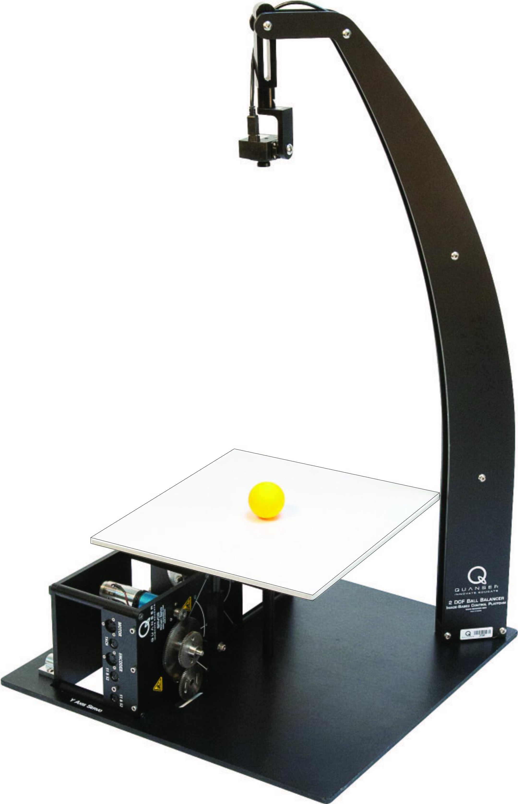
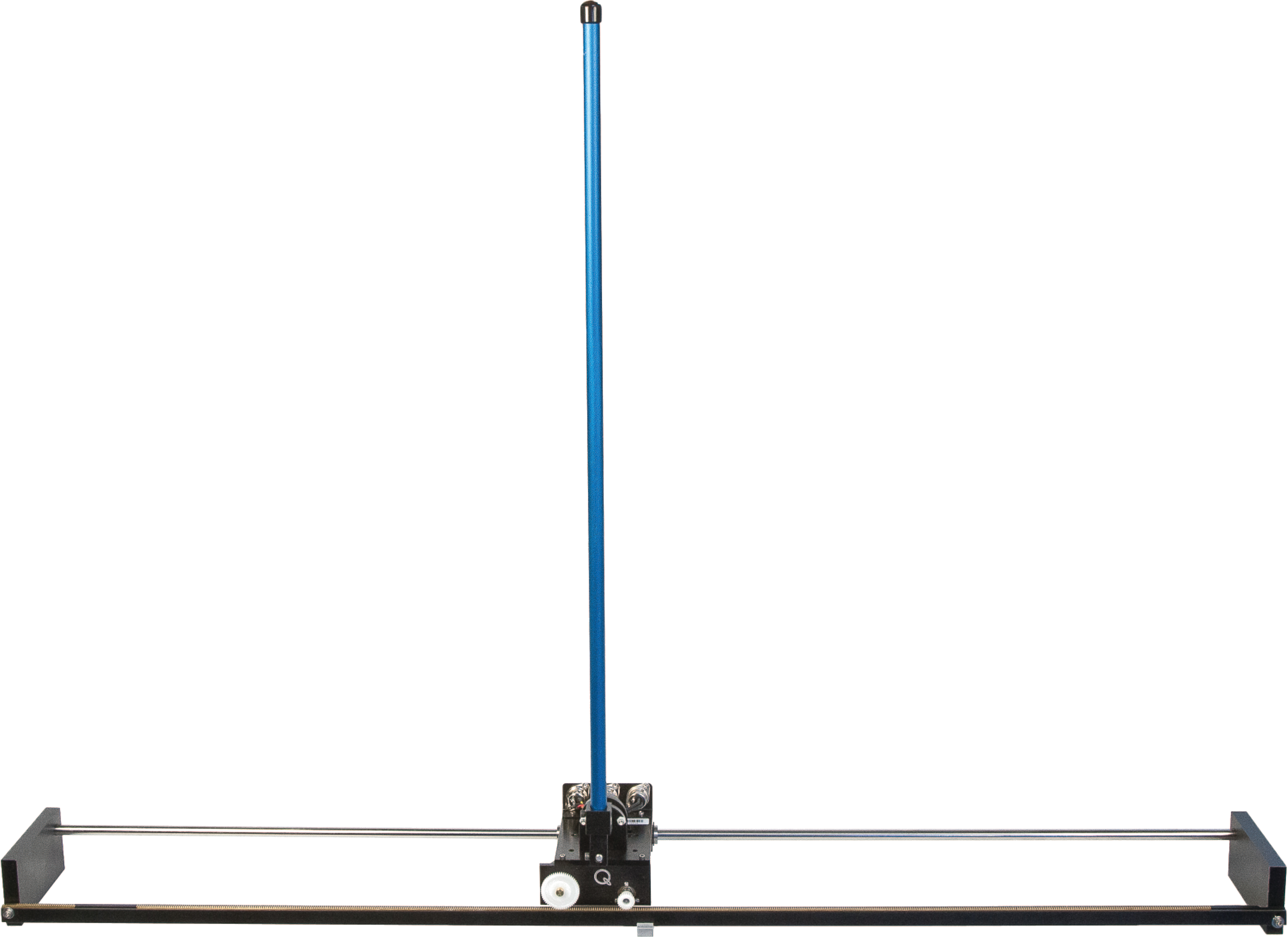
We evaluate SPOTA on two sim-to-real tasks pictured in Figure 1, the Ball-Balancer and the Cart-Pole. The policies obtained by SPOTA are compared against Ensemble Policy Optimization (EPOpt), and (plain) Proximal Policy Optimization (PPO) policies. The goal of the conducted experiments is twofold. First, we want to investigate the applicability of the UCBOG as a quantitative measure of a policy’s transferability. Second, we aim to show that domain randomization enables the sim-to-real transfer of control policies learned by RL algorithms, while methods which only learn from the nominal domain fail to transfer.

4.1 Modeling and Setup Description

Both platforms can be classified as nonlinear under-actuated balancing problems with continuous state and action spaces. The Ball-Balancer’s task is to stabilize the randomly initialized ball at the plate’s center. Given measurements and their first derivatives (obtained by temporal filtering) of the motor shaft angles as well as the ball’s position relative to the plate’s center, the agent controls two servo motors via voltage commands. The rotation of the motor shafts leads, through a kinematic chain, to a change in the plate angles. Finally, the plate’s deflection gets the ball rolling. The Ball-Balancer has an 8D state and a 2D action space. Similarly, the Cart-Pole’s task is to stabilize a pole in the upright position by controlling the cart. Based on measurements and their first derivatives (obtained by temporal filtering) of the pole’s rotation angle as well as the cart position relative to the rail’s center, the agent controls the servo motor driving the cart by sending voltage commands. Accelerating the cart makes the pole rotate around an axis perpendicular to the cart’s direction. The Cart-Pole has a 4D state and a 1D action space. Details on the dynamics of both systems, the reward functions, as well as listings of the domain parameters is given in Appendix A. The nominal models are based on the domain parameter values provided by the manufacturer.

In this paper, both systems have been modeled using the Lagrange formalism and the resulting differential equations are integrated forward in time to simulate the systems. The associated domain parameters are drawn from a probability distribution $\fxi\sim\nu\!\left(\fxi;\fphi\right)$, parameterized by $\fphi$ (e.g., mean, variance). Since randomizing a simulator’s physics parameters is not possible right away, so we developed custom a framework to combine RL and domain randomization. Essentially, the base environment is modified by wrappers which, e.g., vary the mass or delay the actions.

4.2 Experiments Description

The experiments are split into two parts. At first, we examine the evolution of the UCBOG during training (Section 4.3). Next, we compare the transferability of the obtained policies across different realizations of the domain, i.e., simulator (Section 4.3). Finally, we evaluate the policies on the real-world platforms (Section 4.4).

Figure 5: Upper Confidence Bound on the Optimality Gap (UCBOG) and number of candidate solution domain over the iteration count of SPOTA. Every iteration, the number and domains (dashed line) and hence the sample size is increased. The shaded area visualize $\pm 1$ standard deviation across 9 training runs on the simulated Ball-Balancer.

For the experiments on the real Ball-Balancer, we choose 8 initial ball positions equidistant from the plate’s center and place the ball at these points using a PD controller. As soon as a specified accuracy is reached, the evaluated policy is activated for 2000 time steps, i.e., 4 seconds. All experiments on the real Carl-pole start with the cart centered on the rail and the pendulum pole hanging down. After calibration, the pendulum is swung up using an energy-based controller. When the system’s state is within a specified threshold, evaluated policy is executed for 4000 time steps, i.e., 8 seconds.

All policies have been trained in simulation with observation noise to mimic the noisy sensors. To focus on the domain parameters’ influence, we executed the sim-to-sim experiments without observation noise. The policy update at the core of SPOTA, EPOpt, and PPO is done by the Adam optimizer [23]. In the sim-to-sim experiments, the rewards are computed from the ideal states coming from the simulator, while for the sim-to-real experiments the rewards are calculated from the sensor measurements and their time derivatives. The hyper-parameters chosen for the experiments can be found in the Appendix B.

4.3 Sim-to-Sim Results

(a) Ball Balancer – varying ball mass

(b) Ball Balancer – varying ball viscous friction coeff.

(c) Cart-Pole – varying action delay

(d) Cart-Pole – varying motor pinoin radius

Figure 6: Evaluation of the learned control policies on the simulated Ball Balancer (top row) as well as the simulated Cart-Pole (bottom row), (a) varying the ball mass $m_{b}$, (b) the viscous friction coefficient, (c) the action delay $\Delta t_{a}$, and (d) the motor pinion radius $r_{mp}$. Every domain parameter configuration has been evaluated on 360 rollouts with different initial states, synchronized across all policies. The dashed lines mark the nominal parameter values. The solid lines represent the means, and shaded areas show $\pm 1$ standard deviation

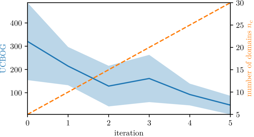
The UCBOG value (32) at each SPOTA iteration depends on several hyper-parameters such as the current number of domains and reference solutions, or the quality of the current iteration’s solution candidate. Figure 5 displays the descent of the UCBOG as well as the growth of the number of domains with the increasing iteration count of SPOTA. As described in Section 2.3.2, the OG and thus the UCBOG only decreases in expectation. Therefore, it can happen that for a specific training run the UCBOG increases from one iteration to the next. Moreover, we observed that the proportion of negative OG estimates (31) increases with progressing iteration count. This observation can be explained by the fact that SPOTA increases the number of domains used during training. Hence the set’s empirical mean approximates the domain parameter distribution $\nu\!\left(\fxi;\fphi\right)$ progressively better, i.e., the candidate and reference solution become more similar. Note, that due to the computational complexity of SPOTA we decided to combine results from experiments with different hyper-parameters in Figure 5.

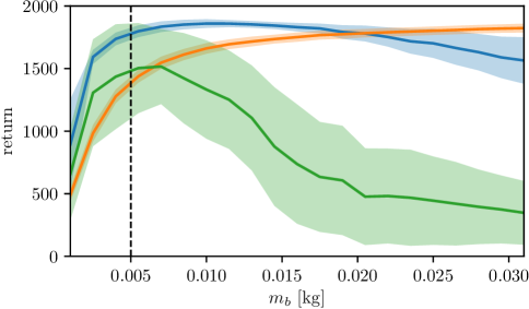
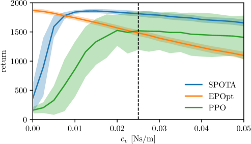
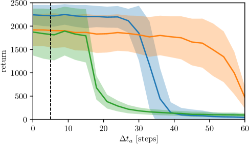
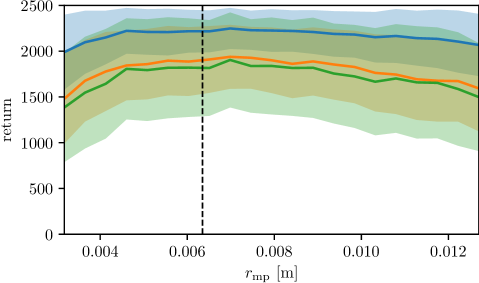
To estimate the robustness w.r.t. model parameter uncertainties, we evaluate policies trained by SPOTA, EPOpt, and PPO under on multiple simulator instances, varying only one domain parameter. The policies’ sensitivity to different parameter values is displayed in the Figure 6. From the Figures 6(a) to 6(c) we can see that the policies learned using (plain) PPO are less robust to changes in the domain parameter values. In contrast, SPOTA and EPOpt are able to maintain their level of performance across a wider range of parameter values. The Figure 6(d) shows the case of a domain parameter to which all policies are equally insensitive. We can also see that EPOpt trades off performance in the nominal domains for performance in more challenging domains (e.g., low friction). This behavior is a consequence of its CVaR-based objective function [11]. Moreover, the results show a higher variance for the PPO policy than for the others. From this, we conclude that domain randomization also acts as regularization mechanism. The final UCBOG value of the evaluated SPOTA policies was $46.42$ for the Ball-Balancer and $55.14$ for the Cart-Pole. Note, that the UCBOG can not be directly observed from the curves in Figure 6, since the UCBOG reflects the gap in performance between the best policy for a specific simulator instance and the candidate policy, whereas the Figure 6 only shows the candidates’ performances.

4.4 Sim-to-Real Results

(a) Ball Balancer – sim-to-real

(b) Cart-Pole – sim-to-real

Figure 7: Evaluation of the learned control policies on (a) the real Ball Balancer and (b) the real Cart-Pole. The results were obtained from 40 rollouts per policy on the Ball Balancer (5 repetitions for 8 different initial ball positions) as well as 10 rollouts (1 initial state) on the Cart-Pole. The dashed lines approximately mark the threshold where the tasks are solved, i.e., the ball is centered in the middle (a), or the pendulum is stabilized upright (b) at the end of the episode.

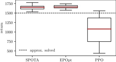
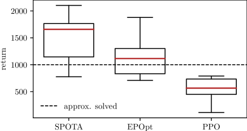
When transferring the policies from simulation to reality without any fine-tuning, we obtain the results reported in Figure 7. The approaches using domain randomization are in most cases able to directly transfer from simulation to reality. In contrast, the policies trained on a singular nominal model using failed to transfer in all but 2 trials on the Ball-Balancer as well as in all trials on the Cart-Pole, even though these policies solved the simulated environments.

Regarding the Ball-Balancer, one explanation why the reported PPO policy did not transfer to the real platform could be the value of the viscous friction coefficient (Figure 6(b)). A possible test for this hypothesis would be to train multiple policies on a range of nominal models with altered viscous friction parameter value, and if these policies still do not transfer, examine the next domain parameter. However, this procedure is redundant and can quickly become prohibitively time-intensive. Concerning the experiments on the Cart-Pole, we observe a larger reality-gap for all policies. We believe that this discrepancy is caused by unmodeled effects between the rack and the cart’s pinion (e.g., the heavy wear and tear of the pinon made out of plastic). Moreover, the variance of the returns is significantly higher. This increase can be largely explained by the variance in the initial states caused by the pre-defined swing-up controller.

A video of the SPOTA policy’s sim-to-real transfer on both platforms can be found at https://www.ias.informatik.tu-darmstadt.de/Team/FabioMuratore.

4.5 Limitations of the Presented Method

The computation of the UCBOG (32), and hence the estimation of the SOB, relies on the relative quality of the candidate and the reference solutions. Therefore, the most notable limitation of the presented method is the optimizer’s ability to reliably solve the SP (5). Since we are interested in the general setting of learning a control policy from a black-box simulator, we chose a model-free RL algorithm. These kind of algorithms can not guarantee to find the globally optimal, or loosely speaking a very good, solution. One way to alleviate this problem is to compute the reference policies from a single domain using methods from control engineering, e.g. a LQR. However, this solution would require an analytic model of the system and a specific type of reward function to preserve comparability between the solutions, e.g. quadratic functions in case of the LQR.

Another limitation of SPOTA is the increased hyper-parameter space which is a direct consequence from the employed (static) domain randomization. In combination with the fact that SPOTA is solving the underlying RL task $(1+n_{G})n_{\text{iter}}$ times, the procedure becomes computationally expensive. One can counter this problem by parallelizing the computation of the reference policies as well as the hyper-parameter search. Both are embarrassingly parallel.

Moreover, SPOTA does not considers uncertainty in the parametrization of the domain parameter distribution $\nu\!\left(\fxi;\fphi\right)$. One possibility to tackle this potential deficiency is to adapt these distributions, as for example done in [17]. Moving from parametric to nonparametric models of the domain parameter distribution is easily possible since SPOTA only requires to sample from them.

Finally, to estimate the SOB, SPOTA assumes that the target domain is covered by the source domain distribution, which can not be guaranteed if the target is a real-world system. However, in the current state-of-the-art there is no way to estimate a policy’s transferability to a domain from an unknown distribution. Due to mentioned assumption, SPOTA’s transferability assessment strongly depends on the simulator’s ability to model the real world.

5 Related Work

In the following, we review excerpts of the literature regarding the transfer of control policies from simulation to reality, the concept of the optimality gap in Stochastic Programs (SP), and the application of randomized physics simulations. This paper is a substantial extension of our previous work [19], adding the derivation of the SOB from the OG (Section 2.2 to 2.4), an outlier rejection component (Algorithm 1), and the method’s first real-world verification using two experiments (Section 4.4).

5.1 Key publications on the Optimality Gap

Hobbs and Hepenstal [2] proved for linear programs that optimization is optimistically biased, given that there are errors in estimating the objective function coefficients. Furthermore, they demonstrated the “optimistic bias” of a nonlinear program, and mentioned the effect of errors on the parameters of linear constraints. The optimization problem introduced in Section 3 belongs to the class of SP for which the assumption required in [2] are guaranteed to hold. The most common approaches to solve convex SP are sample average approximation methods, including: (i) the Multiple Replications Procedure and its derivatives [3, 20] which assess a solution’s quality by comparing with sampled alternative solutions, and (ii) Retrospective Approximation [24, 25] which iteratively improved the solution by lowering the error tolerance. Bastin et al.  [26] extended the existing convergence guarantees from convex to non-convex SP, showing almost sure convergence of the minimizers.

5.2 Prior work on the Reality Gap

Physics simulations have already been used successfully in robot learning. Traditionally, simulators are operating on a single nominal model, which makes the direct transfer of policies from simulation to reality highly vulnerable to model uncertainties and biases. Thus, model-based control in most cases relies on fine-tuned dynamics models.
The mismatch between the simulated and the real world has been addressed by robotics researchers from different viewpoints. Prominent examples are:

1. adding i.i.d. noise to the observations and actions in order to mimic real-world sensor and actuator behavior [1],

2. repeating model generation and selection depending on the short-term state-action history [27],

3. learning a transferability function which maps solutions to a score that quantifies how well the simulation matches the reality [28],

4. adapting the simulator to better match the observed real-world data [17, 29],

5. randomizing the physics simulation’s parameters, and

6. applying adversarial perturbations to the system,

where the last two approaches are particularly related and discussed in the Sections 5.4 and 5.5. The fourth point comprises methods based on system identification, which conceptually differ from the presented method since these seek to find the simulation closest to reality, e.g. minimal prediction error. A recent example in the field of robotics is the work by Hanna and Stone [29], where an action transformation is learned such that the transformed actions applied in simulation have the same effects as applying the original actions had on the real system.

5.3 Required Randomized Simulators

Simulators can be obtained by implementing a set of physical laws or by using general purpose physics engines. The associated physics parameters can be estimated by system identification, which involves executing control policies on the physical platform [30]. Additionally, using the Gauss-Markov theorem one could also compute the parameters’ covariance and hence construct a normal distribution for each domain parameter. Alternatively, the system dynamics can be captured using nonparametric methods like Gaussian processes [31]. It is important to keep in mind, that even if the selected procedure yields a very accurate model parameter estimate, simulators are nevertheless just approximations of the real world and are thus always flawed.

As done in [10, 11, 14, 15, 16] we use the domain parameter distribution as a prior which ensures the physical plausibility of each parameter. Note that specifying this distribution in the current state-of-the-art requires the researcher to make design decisions. Chebotar et al.  [17] presented a promising method which adapts the domain parameter distribution using real-world data in the loop. The main advantage is that this approach alleviates the need for hand-tuning the distributions of the domain parameters, which is currently a significant part of the hyper-parameter search. However, the initial distribution still demands for design decisions. On the downside, the adaptation requires data from the real robot which is considered significantly more expensive to obtain. Since we aim for performing a sim-to-real transfer without using any real-world data, the introduced method only samples from static probability distributions.

5.4 Background on Domain Randomization

There is a large consensus that further increasing the simulator’s accuracy alone will not bridge the reality gap. Instead, the idea of domain randomization has recently gained momentum. The common characteristic of such approaches is the perturbation of the parameters which determine the physics simulator and the state estimation, including but not limited to the system dynamics. While the idea of randomizing the sensors and actuators dates back to at least 1995 [1], the systematic analysis of perturbed simulations in robot RL is a relatively new research direction.

Wang, Fleet, and Hertzmann [32] proposed sampling initial states, external disturbances, goals, as well as actuator noise from probability distributions and learned walking policies in simulation. Regarding robot RL, recent domain randomization methods focus on perturbing the parameters defining the system dynamics. Approaches cover: (i) trajectory optimization on finite model-ensembles [10] (ii) learning a feedforward NN policy for an under-actuated problem [33], (iii) using a risk-averse objective function [11], (iv) employing recurrent NN policies trained with experience replay [15], and (v) optimizing a policy from samples of a model randomly chosen from a set which is repeatedly fitted to real-world data [34]. From the listed approaches [10, 33, 15] were able to cross the reality gap without acquiring samples from the real world.

Moreover, there is a significant amount of work applying domain randomization to computer vision. One example is the work by Tobin et al.  [35] where an object detector for robot grasping is trained using multiple variants of the environment and applied to the real world. The approach presented by Pinto et al.  [14] combines the concepts of randomized environments and actor-critic training, enabling the direct sim-to-real transfer of the abilities to pick, push, or move objects. Sadeghi and Levine [36] achieved the sim-to-real transfer by learning to fly a drone in visually randomized environments. The resulting deep NN policy was able to map from monocular images to normalized 3D drone velocities. In [37], a deep NN was trained to manipulate tissue using randomized vision data and the full state information. By combing generative adversarial networks and domain randomization, Bousmalis et al.  [38] greatly reduced the number of necessary real-world samples for learning a robotic grasping task.

Domain randomization is also related to multi-task learning in the sense that one can view every instance of the randomized source domain as a separate task. In contrast to multi-task learning approaches as presented in [39, 40], a policy learned with SPOTA does not condition on the task. Thus, during execution there is no need to infer the task i.e. domain parameters.

5.5 Randomization Trough Adversarial Perturbations

Another method for learning robust policies in simulation is to apply adversarial disturbances to the training process. Mandlekar et al.  [12] proposed physically plausible perturbations by randomly deciding when to add a rescaled gradient of the expected return. Pinto et al.  [13] introduced the idea of a second agent whose goal is to hinder the first agent from fulfilling its task. Both agents are trained simultaneously and make up a zero-sum game. In general, adversarial approaches may provide a particularly robust policy. However, without any further restrictions, it is always possible create scenarios in which the protagonist agent can never win, i.e., the policy will not learn the task.

6 Conclusion

We proposed a novel measure of the Simulation Optimization Bias (SOB) for quantifying the transferability of an arbitrary policy learned from a randomized source domain to an unknown target domain from the same domain parameter distribution. Based on this measure of the SOB, we developed a policy search meta-algorithm called Simulation-based Policy Optimization with Transferability Assessment (SPOTA). This gist of SPOTA is to iteratively increase the number of domains and thereby the sample size per iteration until an approximate probabilistic guarantee on the optimality gap holds. The required approximation of the optimality gap is obtained by comparing the current candidate policy against multiple reference policies evaluated in the associated reference domains. After training, we can make an approximation of the resulting policy’s suboptimality when transferring to a different domain from the same (source) distribution. To verify our approach we conducted two sim-to-real experiments on second order nonlinear continuous control systems. The results showed that SPOTA policies were able to directly transfer from simulation to reality while the baseline without domain randomization failed.

In the future we will investigate different strategies for sampling the domain parameters to replace the i.i.d. sampling from hand-crafted distributions. One idea is to employ Bayesian optimization for selecting the next set of domain parameters. Thus, the domain randomization could be executed according to an objective, and potentially increase sample-efficiency. Furthermore, we plan to devise a formulation which frames domain randomization and policy search in one optimization problem. This would allow for an joint treatment of finding a policy and matching the simulator to the real world.

Appendix A Modeling Details on the Platforms

The Ball-Balancer is modeled as a nonlinear second-order dynamical system

$$\ddot{\fs}=\begin{bmatrix}\ddot{\theta}_{x}\\ \ddot{\theta}_{y}\\ \ddot{x}_{b}\\ \ddot{y}_{b}\end{bmatrix}=\begin{bmatrix}(A_{m}V_{x}-B_{v}\dot{\theta}_{x})/J_{eq}\\ (A_{m}V_{y}-B_{v}\dot{\theta}_{y})/J_{eq}\\ (-c_{v}\dot{x}_{b}r_{b}^{2}-J_{b}r_{b}\ddot{\alpha}+m_{b}x_{b}\dot{\alpha}^{2}r_{b}^{2}\\ \quad+\leavevmode\nobreak\ c_{kin}m_{b}gr_{b}^{2}\mathrm{sin}\!\left(\theta_{x}\right))/\zeta\\ (-c_{v}\dot{y}_{b}r_{b}^{2}-J_{b}r_{b}\ddot{\beta}+m_{b}y_{b}\dot{\beta}^{2}r_{b}^{2}\\ \quad+\leavevmode\nobreak\ c_{kin}m_{b}gr_{b}^{2}\mathrm{sin}\!\left(\theta_{y}\right))/\zeta\end{bmatrix},$$ (34)

with the motor shaft angles $\theta_{x}$ and $\theta_{y}$, the ball positions relative to the place center $x_{b}$ and $y_{b}$, the plate angle $\beta$ and $\alpha$ around the $x$ and $y$ axis, and the commanded motor voltages ${\fa^{\textsf{T}}=\left[V_{x},V_{y}\right]}$. To model the gears’ backlash, we set all voltage values between $V_{thold,-}$ and $V_{thold,+}$ to zero. These threshold values have been determined in separate experiments for both servo motors. The Ball-Balancer’s domain parameters as well as the ones derived from them are listed in Table IV. For the Ball-Balancer’s we define the reward function as

$$r\!\left(\fs_{t},\fa_{t}\right)=\mathrm{exp}\left(c\left(\fs_{t}^{\textsf{T}}\fQ_{BB}\fs_{t}+\fa_{t}^{\textsf{T}}\fR_{BB}\fa_{t}\right)\right)$$ (35)

$$\text{with }c=\frac{\mathrm{ln}\left(r_{min}\right)}{\max_{\fs\in\mathcal{S}_{\bar{\fxi}},\fa\in\mathcal{A}_{\bar{\fxi}}}\fs^{\textsf{T}}\fQ_{BB}\fs+\fa^{\textsf{T}}\fR_{BB}\fa}.$$ (36)

Given a lower bound for the reward $r_{min}\in[0,1]$, the reward function above yields values within $[r_{min},1]$ at each time step. We found that the scaling constant $c<0$ is beneficial for the learning procedure, since it prohibits the reward from going to zero too quickly. The constant’s denominator can be easily inferred from the nominal state and action set’s boundaries.

The Cart-Pole is modeled as a nonlinear second-order dynamical system given by the solution of

$$\begin{bmatrix}m_{p}+J_{eq}&m_{p}l_{p}\mathrm{cos}\!\left(\alpha\right)\\ m_{p}l_{p}\mathrm{cos}\!\left(\alpha\right)&J_{p}+m_{p}l_{p}^{2}\end{bmatrix}\begin{bmatrix}\ddot{x}\\ \ddot{\alpha}\end{bmatrix}=$$ (37)

$$\begin{bmatrix}F-m_{p}l_{p}\mathrm{sin}\!\left(\alpha\right)\dot{\alpha}^{2}-B_{eq}\dot{x}\\ -m_{p}l_{p}g\mathrm{sin}\!\left(\alpha\right)-B_{p}\dot{\alpha}\\ \end{bmatrix},$$ (38)

where the commanded motor voltage $V$ is encapsulated in

$$F=\frac{\eta_{g}K_{g}k_{m}}{R_{m}r_{mp}}\left(\frac{\eta_{m}V-K_{g}k_{m}\dot{x}}{r_{mp}}\right).$$ (39)

The system’s state $\fs$ is given by the cart’s position $x$ and the pole’s angle $\alpha$, which are defined to be zero at the rail’s center and hanging down vertically, respectively. The Cart-Pole’s domain parameters as well as the parameters derived from them are listed in Table V. Similar to the Ball-Balancer, the Cart-Pole’s reward function is based on an exponentiated quadratic cost

$$r\!\left(\fs_{t},a_{t}\right)=\mathrm{exp}\left(-\left(\fs_{t}^{\textsf{T}}\fQ_{CP}\fs_{t}+a_{t}^{\textsf{T}}R_{CP}a_{t}\right)\right).$$ (40)

Thus, the reward is in range $]0,1]$ for every time step.

Appendix B Parameter values for the experiments

Table II: Domain parameter values for the illustrative example. Additional (domain-independent) parameters are $m=$1\text{\,}\mathrm{kg}\text{/}$$ and $\phi=0.7$.

Domain	$g_{i}[$\mathrm{m}\mathrm{/}\sec\mathrm{{}^{2}}$]$	$k_{i}[$\mathrm{N}\mathrm{/}\mathrm{m}$]$	$x_{i}[$\mathrm{m}\text{/}$]$
Mars	$3.71$	$1000$	$0.5$
Venus	$8.87$	$3000$	$1.5$

Table III: Hyper-parameter values for the experiments in Section 4. All simulator parameters were randomized such that they stayed physically plausible. We use $n$ as shorthand for ${n_{c}}$ or ${n_{r}}$ depending on the context.

Hyper-parameter	Value
PolOpt	PPO
policy architecture	FNN $16$-$16$ with tan-h
optimizer	Adam
learning rate	$110-4$
number of iterations $n_{\text{iter}}$	$400$
max. steps per episode $T$	Ball-Balancer: $2000$
	Cart-Pole: $2500$
step size $\Delta t$	$0.002\text{\,}\mathrm{s}\text{/}$
temporal discount $\gamma$	$0.999$
$\lambda$ (andvantage estimation)	$0.95$
initial ${n_{c}}$	$5$
initial ${n_{r}}$	$1$
NonDecrSeq	$n_{k+1}\leftarrow\lfloor n_{0}(k+1)\rfloor$
rollouts per domain parameter $n_{\tau}$	$10$
batch size	$\left\lceil T/\Delta t\right\rceil n_{\tau}n$ steps
number of reference solutions $n_{G}$	$20$
rollouts per initial state $n_{J}$	Ball-Balancer: $120$
	Cart-Pole: $50$
confidence parameter $\alpha$	$0.05$
threshold of trust $\beta$	Ball-Balancer: $50$
	Cart-Pole: $60$
number of bootstrap replications $B$	$1000$
CVaR parameter $\epsilon$ (EPOpt)	$0.2$
$r_{min}$	$10^{-4}$
$\fQ_{bb}$	$\textrm{diag}(1,1,$5103$,$5103$,\dots$
	$$110-2$,$110-2$,$510-2$,$510-2$)$
$\fR_{bb}$	$\mathrm{diag}($110-3$,$110-3$)$
$\fQ_{cp}$	$\textrm{diag}($10$,$1103$,$510-2$,$510-3$)$
$R_{cp}$	$110-4$
obs. noise std for linear pos	$510-3\text{\,}\mathrm{m}\text{/}$
obs. noise std for linear vel	$0.05\text{\,}\mathrm{m}\text{/}\mathrm{s}$
obs. noise std for angular pos	$0.5\text{\,}\mathrm{\SIUnitSymbolDegree}\text{/}$
obs. noise std for angular vel	$2.0\text{\,}\mathrm{\SIUnitSymbolDegree}\text{/}\mathrm{s}$

Table IV: The domain parameter distributions and derived parameters for the Ball-Balancer (Figure 1 left). All parameters were randomized such that they stayed physically plausible. Normal distributions are parameterized with mean and standard deviation, uniform distributions with lower and upper bound. The lines separate the randomized domain parameters from the ones depending on these.

Parameter	Distribution	Unit
gravity constant	$\mathcal{\mathcal{N}}\left(g\big{|}$9.81$,$1.962$\right)$	$[$\mathrm{k}\mathrm{g}$]$
ball mass	$\mathcal{\mathcal{N}}\left(m_{b}\big{|}$510-3$,$610-4$\right)$	$[$\mathrm{k}\mathrm{g}$]$
ball radius	$\mathcal{\mathcal{N}}\left(r_{b}\big{|}$1.9610-2$,$3.9310-3$\right)$	$[$\mathrm{m}$]$
plate length	$\mathcal{\mathcal{N}}\left(l_{p}\big{|}$0.275$,$5.510-2$\right)$	$[$\mathrm{m}$]$
kinematic leverage arm	$\mathcal{\mathcal{N}}\left(r_{kin}\big{|}$2.5410-2$,$3.0810-3$\right)$	$[$\mathrm{m}$]$
gear ratio	$\mathcal{\mathcal{N}}\left(K_{g}\big{|}70,14\right)$	$[-]$
gearbox efficiency	$\mathcal{\mathcal{U}}\left(\eta_{g}\big{|}$1.0$,$0.6$\right)$	$[-]$
motor efficiency	$\mathcal{\mathcal{U}}\left(\eta_{m}\big{|}$0.89$,$0.49$\right)$	$[-]$
load moment of inertia	$\mathcal{\mathcal{N}}\left(J_{l}\big{|}$5.2810-5$,$1.0610-5$\right)$	$[$\mathrm{kg}\text{\,}{\mathrm{m}}^{2}\text{/}$]$
motor moment of inertia	$\mathcal{\mathcal{N}}\left(J_{m}\big{|}$4.6110-7$,$9.2210-8$\right)$	$[$\mathrm{kg}\text{\,}{\mathrm{m}}^{2}\text{/}$]$
motor torque constant	$\mathcal{\mathcal{N}}\left(k_{m}\big{|}$7.710-3$,$1.5210-3$\right)$	$[$\mathrm{N}\text{\,}\mathrm{m}\text{/}\mathrm{A}$]$
motor armature resistance	$\mathcal{\mathcal{N}}\left(R_{m}\big{|}$2.6$,$0.52$\right)$	$[$\mathrm{\SIUnitSymbolOhm}\text{/}$]$
motor viscous damping coeff. w.r.t. load	$\mathcal{\mathcal{U}}\left(B_{\text{eq}}\big{|}$0.15$,$3.7510-3$\right)$	$[$\mathrm{N}\text{\,}\mathrm{m}\text{\,}\mathrm{s}\text{/}$]$
ball/plate viscous friction coeff.	$\mathcal{\mathcal{U}}\left(c_{v}\big{|}$5.010-2$,$1.2510-3$\right)$	$[-]$
positive voltage threshold x servo	$\mathcal{\mathcal{U}}\left(V_{thold,x+}\big{|}$0.353$,$8.8410-2$\right)$	$[$\mathrm{V}\text{/}$]$
negative voltage threshold x servo	$\mathcal{\mathcal{U}}\left(V_{thold,x-}\big{|}$-8.9010-2$,$-2.2210-3$\right)$	$[$\mathrm{V}\text{/}$]$
positive voltage threshold y servo	$\mathcal{\mathcal{U}}\left(V_{thold,y+}\big{|}$0.290$,$7.2510-2$\right)$	$[$\mathrm{V}\text{/}$]$
negative voltage threshold y servo	$\mathcal{\mathcal{U}}\left(V_{thold,y-}\big{|}$-7.3010-2$,$-1.8310-2$\right)$	$[$\mathrm{V}\text{/}$]$
offset x servo	$\mathcal{\mathcal{U}}\left(\Delta\theta_{x}\big{|}-5,5\right)$	$[$\deg$]$
offset y servo	$\mathcal{\mathcal{U}}\left(\Delta\theta_{y}\big{|}-5,5\right)$	$[$\deg$]$
action delay	$\mathcal{\mathcal{U}}\left(\Delta t_{a}\big{|}0,30\right)$	$[\mathrm{steps}]$
kinematic constant	$c_{kin}=2r_{\text{kin}}/l_{p}$	$[-]$
combined motor constant	$A_{m}=\eta_{g}K_{g}\eta_{m}k_{m}/R_{m}$	$[$\mathrm{N}\text{\,}\mathrm{m}\text{/}\mathrm{V}$]$
combined rotary damping coefficient	$B_{v}=\eta_{g}K_{g}^{2}\eta_{m}k_{m}^{2}/R_{m}+B_{\text{eq}}$	$[$\mathrm{N}\text{\,}\mathrm{m}\text{\,}\mathrm{s}\text{/}$]$
combined rotor inertia	$J_{eq}=\eta_{g}K_{g}^{2}J_{m}+J_{l}$	$[$\mathrm{kg}\text{\,}{\mathrm{m}}^{2}\text{/}$]$
ball inertia about CoM	$J_{b}=2/5m_{b}r_{b}^{2}$	$[$\mathrm{kg}\text{\,}{\mathrm{m}}^{2}\text{/}$]$
combined ball inertia	$\zeta=m_{b}r_{b}^{2}+J_{b}$	$[$\mathrm{kg}\text{\,}{\mathrm{m}}^{2}\text{/}$]$

Table V: The domain parameter distributions and derived parameters for the Cart-Pole (Figure 1 right). All parameters were randomized such that they stayed physically plausible. Normal distributions are parameterized with mean and standard deviation, uniform distributions with lower and upper bound. The lines separate the randomized domain parameters from the ones depending on these.

Parameter	Distribution	Unit
gravity constant	$\mathcal{\mathcal{N}}\left(g\big{|}$9.81$,$1.962$\right)$	$[$\mathrm{k}\mathrm{g}$]$
cart mass	$\mathcal{\mathcal{N}}\left(m_{c}\big{|}$0.38$,$0.076$\right)$	$[$\mathrm{k}\mathrm{g}$]$
pole mass	$\mathcal{\mathcal{N}}\left(m_{p}\big{|}$0.127$,$2.5410-2$\right)$	$[$\mathrm{k}\mathrm{g}$]$
half pole length	$\mathcal{\mathcal{N}}\left(l_{p}\big{|}$0.089$,$1.7810-2$\right)$	$[$\mathrm{m}$]$
rail length	$\mathcal{\mathcal{N}}\left(l_{r}\big{|}$0.814$,$0.163$\right)$	$[$\mathrm{m}$]$
motor pinion radius	$\mathcal{\mathcal{N}}\left(r_{mp}\big{|}$6.3510-3$,$1.2710-3$\right)$	$[$\mathrm{m}$]$
gear ratio	$\mathcal{\mathcal{N}}\left(K_{g}\big{|}3.71,0\right)$	$[-]$
gearbox efficiency	$\mathcal{\mathcal{U}}\left(\eta_{g}\big{|}$1.0$,$0.8$\right)$	$[-]$
motor efficiency	$\mathcal{\mathcal{U}}\left(\eta_{m}\big{|}$1.0$,$0.8$\right)$	$[-]$
motor moment of inertia	$\mathcal{\mathcal{N}}\left(J_{m}\big{|}$3.910-7$,$0$\right)$	$[$\mathrm{kg}\text{\,}{\mathrm{m}}^{2}\text{/}$]$
motor torque constant	$\mathcal{\mathcal{N}}\left(k_{m}\big{|}$7.6710-3$,$1.5210-3$\right)$	$[$\mathrm{N}\text{\,}\mathrm{m}\text{/}\mathrm{A}$]$
motor armature resistance	$\mathcal{\mathcal{N}}\left(R_{m}\big{|}$2.6$,$0.52$\right)$	$[$\mathrm{\SIUnitSymbolOhm}\text{/}$]$
motor viscous damping coeff. w.r.t. load	$\mathcal{\mathcal{U}}\left(B_{eq}\big{|}$5.4$,$0$\right)$	$[$\mathrm{N}\text{\,}\mathrm{s}\text{/}\mathrm{m}$]$
pole viscous friction coeff.	$\mathcal{\mathcal{U}}\left(B_{p}\big{|}$2.410-3$,$0$\right)$	[$\mathrm{N}\text{\,}\mathrm{s}\text{/}$]
action delay	$\mathcal{\mathcal{U}}\left(\Delta t_{a}\big{|}0,10\right)$	$[\mathrm{steps}]$
pole rotary inertia about pivot point	$J_{p}=1/3m_{p}l_{p}^{2}$	$[$\mathrm{kg}\text{\,}{\mathrm{m}}^{2}\text{/}$]$
combined linear inertia	$J_{eq}=m_{c}+(\eta_{g}K_{g}^{2}J_{m})/r_{mp}^{2}$	$[$\mathrm{kg}\text{/}$]$

References

- [1] N. Jakobi, P. Husbands, and I. Harvey, “Noise and the reality gap: The use of simulation in evolutionary robotics,” in Advances in Artificial Life, Granada, Spain, June 4-6, 1995, pp. 704–720.
- [2] B. F. Hobbs and A. Hepenstal, “Is optimization optimistically biased?” Water Resources Research, vol. 25, no. 2, pp. 152–160, 1989.
- [3] W. Mak, D. P. Morton, and R. K. Wood, “Monte carlo bounding techniques for determining solution quality in stochastic programs,” Oper. Res. Lett., vol. 24, no. 1-2, pp. 47–56, 1999.
- [4] “Quanser platforms,” www.quanser.com/products/.
- [5] V. Mnih, K. Kavukcuoglu, D. Silver, A. A. Rusu, J. Veness, M. G. Bellemare, A. Graves, M. A. Riedmiller, A. Fidjeland, G. Ostrovski, S. Petersen, C. Beattie, A. Sadik, I. Antonoglou, H. King, D. Kumaran, D. Wierstra, S. Legg, and D. Hassabis, “Human-level control through deep reinforcement learning,” Nature, vol. 518, no. 7540, pp. 529–533, 2015.
- [6] D. Silver, J. Schrittwieser, K. Simonyan, I. Antonoglou, A. Huang, A. Guez, T. Hubert, L. Baker, M. Lai, A. Bolton, et al., “Mastering the game of go without human knowledge,” Nature, vol. 550, no. 7676, p. 354, 2017.
- [7] T. P. Lillicrap, J. J. Hunt, A. Pritzel, N. Heess, T. Erez, Y. Tassa, D. Silver, and D. Wierstra, “Continuous control with deep reinforcement learning,” in ICLR, San Juan, Puerto Rico, May 2-4, 2016.
- [8] J. Schulman, F. Wolski, P. Dhariwal, A. Radford, and O. Klimov, “Proximal policy optimization algorithms,” ArXiv e-prints, 2017.
- [9] A. A. Rusu, M. Vecerik, T. Rothörl, N. Heess, R. Pascanu, and R. Hadsell, “Sim-to-real robot learning from pixels with progressive nets,” in CoRL, Mountain View, California, USA, November 13-15, 2017, pp. 262–270.
- [10] I. Mordatch, K. Lowrey, and E. Todorov, “Ensemble-cio: Full-body dynamic motion planning that transfers to physical humanoids,” in IROS, Hamburg, Germany, September 28 - October 2, 2015, pp. 5307–5314.
- [11] A. Rajeswaran, K. Lowrey, E. Todorov, and S. M. Kakade, “Towards generalization and simplicity in continuous control,” in NIPS, Long Beach, CA, USA, 4-9 December, 2017, pp. 6553–6564.
- [12] A. Mandlekar, Y. Zhu, A. Garg, L. Fei-Fei, and S. Savarese, “Adversarially robust policy learning: Active construction of physically-plausible perturbations,” in IROS, Vancouver, BC, Canada, September 24-28, 2017, pp. 3932–3939.
- [13] L. Pinto, J. Davidson, R. Sukthankar, and A. Gupta, “Robust adversarial reinforcement learning,” in ICML, Sydney, NSW, Australia, August 6-11. PMLR, 2017, pp. 2817–2826.
- [14] L. Pinto, M. Andrychowicz, P. Welinder, W. Zaremba, and P. Abbeel, “Asymmetric actor critic for image-based robot learning,” in RSS, Pittsburgh, Pennsylvania, USA, June 26-30, 2018.
- [15] X. B. Peng, M. Andrychowicz, W. Zaremba, and P. Abbeel, “Sim-to-real transfer of robotic control with dynamics randomization,” in ICRA, Brisbane, Australia, May 21-25, 2018, pp. 1–8.
- [16] W. Yu, J. Tan, C. K. Liu, and G. Turk, “Preparing for the unknown: Learning a universal policy with online system identification,” in RSS, Cambridge, Massachusetts, USA, July 12-16, 2017.
- [17] Y. Chebotar, A. Handa, V. Makoviychuk, M. Macklin, J. Issac, N. D. Ratliff, and D. Fox, “Closing the sim-to-real loop: Adapting simulation randomization with real world experience,” in ICRA, Montreal, QC, Canada, May 20-24, 2019, pp. 8973–8979.
- [18] OpenAI, M. Andrychowicz, B. Baker, M. Chociej, R. Jozefowicz, B. McGrew, J. Pachocki, A. Petron, M. Plappert, G. Powell, A. Ray, J. Schneider, S. Sidor, J. Tobin, P. Welinder, L. Weng, and W. Zaremba, “Learning dexterous in-hand manipulation,” ArXiv e-prints, vol. 1808.00177, 2018.
- [19] F. Muratore, F. Treede, M. Gienger, and J. Peters, “Domain randomization for simulation-based policy optimization with transferability assessment,” in CoRL, Zürich, Switzerland, 29-31 October, 2018, pp. 700–713.
- [20] G. Bayraksan and D. P. Morton, “Assessing solution quality in stochastic programs,” Math. Program., vol. 108, no. 2-3, pp. 495–514, 2006.
- [21] B. Efron, “Bootstrap methods: another look at the jackknife,” Annals of Statistics, pp. 1–26, 1979.
- [22] T. J. DiCiccio and B. Efron, “Bootstrap confidence intervals,” Statistical Science, pp. 189–212, 1996.
- [23] D. P. Kingma and J. Ba, “Adam: a method for stochastic optimization,” in ICLR, San Diego, CA, USA, May 7-9, 2015.
- [24] R. Pasupathy and B. W. Schmeiser, “Retrospective-approximation algorithms for the multidimensional stochastic root-finding problem,” ACM Trans. Model. Comput. Simul., vol. 19, no. 2, pp. 5:1–5:36, 2009.
- [25] S. Kim, R. Pasupathy, and S. G. Henderson, “A guide to sample average approximation,” in Handbook of Simulation Optimization. Springer, 2015, pp. 207–243.
- [26] F. Bastin, C. Cirillo, and P. L. Toint, “Convergence theory for nonconvex stochastic programming with an application to mixed logit,” Math. Program., vol. 108, no. 2-3, pp. 207–234, 2006.
- [27] J. Bongard, V. Zykov, and H. Lipson, “Resilient machines through continuous self-modeling,” Science, vol. 314, no. 5802, pp. 1118–1121, 2006.
- [28] S. Koos, J. Mouret, and S. Doncieux, “The transferability approach: Crossing the reality gap in evolutionary robotics,” IEEE Trans. Evol. Comput., vol. 17, no. 1, pp. 122–145, 2013.
- [29] J. P. Hanna and P. Stone, “Grounded action transformation for robot learning in simulation,” in AAAI, San Francisco, California, USA, February 4-9, 2017, pp. 3834–3840.
- [30] R. Isermann and M. Münchhof, Identification of Dynamic Systems: An Introduction with Applications. Springer Science & Business Media, 2010.
- [31] C. E. Rasmussen and C. K. I. Williams, Gaussian processes for machine learning, ser. Adaptive computation and machine learning. MIT Press, 2006.
- [32] J. M. Wang, D. J. Fleet, and A. Hertzmann, “Optimizing walking controllers for uncertain inputs and environments,” ACM Trans. Graph., vol. 29, no. 4, pp. 73:1–73:8, 2010.
- [33] R. Antonova and S. Cruciani, “Unlocking the potential of simulators: Design with RL in mind,” ArXiv e-prints, 2017.
- [34] T. Kurutach, I. Clavera, Y. Duan, A. Tamar, and P. Abbeel, “Model-ensemble trust-region policy optimization,” in ICLR, Vancouver, BC, Canada, April 30 - May 3, 2018.
- [35] J. Tobin, R. Fong, A. Ray, J. Schneider, W. Zaremba, and P. Abbeel, “Domain randomization for transferring deep neural networks from simulation to the real world,” in IROS, Vancouver, BC, Canada, September 24-28, 2017, pp. 23–30.
- [36] F. Sadeghi and S. Levine, “CAD2RL: real single-image flight without a single real image,” in RSS, Cambridge, Massachusetts, USA, July 12-16, 2017.
- [37] J. Matas, S. James, and A. J. Davison, “Sim-to-real reinforcement learning for deformable object manipulation,” in CoRL, Zürich, Switzerland, 29-31 October, 2018, pp. 734–743.
- [38] K. Bousmalis, A. Irpan, P. Wohlhart, Y. Bai, M. Kelcey, M. Kalakrishnan, L. Downs, J. Ibarz, P. Pastor, K. Konolige, S. Levine, and V. Vanhoucke, “Using simulation and domain adaptation to improve efficiency of deep robotic grasping,” in ICRA, Brisbane, Australia, May 21-25, 2018, pp. 4243–4250.
- [39] M. P. Deisenroth, P. Englert, J. Peters, and D. Fox, “Multi-task policy search for robotics,” in ICRA, Hong Kong, China, May 31 - June 7, 2014, pp. 3876–3881.
- [40] M. Andrychowicz, D. Crow, A. Ray, J. Schneider, R. Fong, P. Welinder, B. McGrew, J. Tobin, P. Abbeel, and W. Zaremba, “Hindsight experience replay,” in NIPS, Long Beach, CA, USA, 4-9 December, 2017, pp. 5048–5058.