On the counting of $O(N)$ tensor invariants

Abstract

$O(N)$ invariants are the observables of real tensor models. We use regular colored graphs to represent these invariants, the valence of the vertices of the graphs relates to the tensor rank. We enumerate $O(N)$ invariants as $d$-regular graphs, using permutation group techniques. We also list their generating functions and give (software) algorithms computing their number at an arbitrary rank and an arbitrary number of vertices. As an interesting property, we reveal that the algebraic structure which organizes these invariants differs from that of the unitary invariants. The underlying topological field theory formulation of the rank $d$ counting shows that it corresponds to counting of coverings of the $d-1$ cylinders sharing the same boundary circle and with $d$ defects. At fixed rank and fixed number of vertices, an associative semi-simple algebra with dimension the number of invariants naturally emerges from the formulation. Using the representation theory of the symmetric group, we enlighten a few crucial facts: the enumeration of $O(N)$ invariants gives a sum of constrained Kronecker coefficients; there is a representation theoretic orthogonal base of the algebra that reflects its dimension; normal ordered 2-pt correlators of the Gaussian models evaluate using permutation group language, and further, via representation theory, these functions provide other representation theoretic orthogonal bases of the algebra.

1 Introduction

Since their inception [1, 2, 3], random tensor models offer a framework for studying random discrete geometries as they aim at extending the success of matrix models [4] in describing 2D quantum gravity, to higher dimensions. The main goal of this approach is to devise a transition of discrete geometries to continuum geometries in any dimension. It is however only recently that random tensor models have witnessed significant progress [5] with the advent of a new large $N$ expansion generalizing ‘t Hooft genus expansion [6] for higher dimensional pseudo-manifolds. The existence of a large $N$ expansion for tensors [7] naturally unveiled several analytical results, among which the discovery of their critical behavior (branched polymers [8, 9]), the universality property of random tensors [10], and the discovery of new families of renormalizable non-local quantum field theories with interesting UV [11, 12, 13] and nonperturbative behaviors supporting the discovery of new universality classes for gravity [14, 15, 16].

More recently, and quite unexpectedly, tensor models become the center of new attention in condensed matter physics: the dominant contributions of the so-called Sachdev-Ye-Kitaev (SYK) model [17, 18] in the large mode expansion of the disorder match with the large $N$ expansion of a quantum mechanical tensor model without disorder [19]. For its deep connections with black hole physics and AdS/CFT correspondence, the SYK model embodies a vibrant topic of research. The conjunction of tensor and SYK models has incidentally produced a new fast-evolving field on which a growing community is working.

Several, if not all of these studies, heavily rest on the understanding of the combinatorics of Feynman graphs and observables of tensor models. To that extent, the investigations of tensor models have produced a wealth of results. We will focus on two particular contributions on tensor model graphs that the present work extends.

In [20], the authors worked out the enumeration of the unitary invariants, as observables in complex tensor models. One way of comprehending the theory space of rank $d$ complex tensor models is to specify its set of observables. The latter are merely $U(N)^{\otimes d}$ invariants (at time, we simply call them $U(N)$ or complex tensor invariants). A convenient manner to represent $U(N)$ invariants defines as a canonical mapping to $d$-regular bipartite colored graphs [21]. Stated in this way, the inventory of tensor invariants formulates by uniquely using permutation groups. One should record that these symmetry group techniques and its representation theory have been developed during the last years [22]–[33]. They turned out to be powerful, flexible and versatile enough to address diverse enumeration problems and bijections from scalar field theory, matrix models, to gauge (QED, 2D and 4D Yang-Mills) and string theories. In physics, for instance, they brighten the half-BPS sector of ${\mathcal{N}}=4$ SYM [22]–[27]. Moreover, unforeseen correspondences arise from these studies, for instance, counting Feynman graphs in $\phi^{4}$ scalar field theory relates to string theory on a cylinder or listing Feynman graphs of QED relates to the counting of ribbon graphs [26]. These correspondences emerge from another interface playing a hinge role between enumeration problems: via the Burnside lemma, with each enumeration problem using the symmetric group (and its subgroups), we can associate a Topological Field Theory on a 2-complex (named TFT₂) with gauge group given by the symmetric group (and its subgroups). Such a formulation also unfolds multiple interpretations of the counting formulae with links with the theory of covering spaces in algebraic and complex geometry (see references in [26]).

The reference [20] establishes several enumeration formulae pertaining to observables of complex tensor models. Using the Burnside lemma, one recasts that the enumeration of $U(N)$ invariants into a partition of a permutation lattice gauge field theory, a TFT₂. It is via this mapping that one elucidates that counting unitary invariants corresponds to counting branched covers of the 2-sphere. Branched covers are well known objects in algebraic and complex geometry [34], in topological string theory, and in dimension 2, they correspond to complex maps [25]. Thus, there is an underlying geometry inherited by tensor models from the TFT₂ formulation that still needs to be understood. There is however a proviso: the counting formulae are valid when the size $N$ of the tensor indices are larger than the number of tensors convoluted. More generally, one should resort to a more careful study [32, 33].

The study of tensor invariants has a follow-up in [35]. Their equivalent classes are viewed as the base elements of a vector space $\mathcal{K}_{d}(n)$, a subspace of ${\mathbb{C}}(S_{n})^{\otimes d}$, the rank $d$ group algebra of the symmetric group $S_{n}$. $\mathcal{K}_{d}(n)$ shows stability under an associative product, and it is endowed with a non-degenerate pairing. Therefore, at a fixed rank $d$ and fixed number of vertices $n$, tensor invariants span a semi-simple algebra. (Note that, importantly, other algebraic structures could set up on tensor invariants [36, 37, 38]. The above structure is however unique, up to isomorphism.) As a consequence of the Wedderburn-Artin theorem, any semi-simple algebra decomposes as a sum of irreducible matrix subalgebras. The representation theory of the symmetric group sheds more light on the remaining analysis as it enables to reach the Wedderburn-Artin matrix decomposition of the algebra of tensor observables: the dimension of the algebra is a sum of squares of the Kronecker coefficients (these are multiplicity dimensions in the decomposition of a tensor product of representations in irreps; Kronecker coefficients are still under active investigation in Combinatorics and Computational Complexity Theory, see, for instance, [39, 40] and more references therein), each square matching exactly the dimension of a matrix subalgebra. The orthogonal bases of the algebra and its matrix subalgebras have been worked out, meanwhile the Gaussian 2pt-correlators also provide new representation theoretic orthogonal bases.

In this paper, we consider $O(N)$ tensor models and their observables and investigate if they support the same previous enumeration and algebraic analysis. Fleshed out the first time in [41], such models extended the large $N$ expansion to real tensors. The graphs that determine the $O(N)$ invariants keep the edge coloring but are not bipartite. This naturally leads to a class of observables, wider than that of the $U(N)$ tensor models, by including those that are not orientable. To enumerate $O(N)$ invariants, we use a standard counting recipe: we use tuples of permutations on which act permutation (sub)groups that define equivalence classes. We then count the points in the resulting a double coset space. The equivalence relation in the present setting is radically different from the $U(N)$ situation and requires more work to obtain a valuable counting formula. With their generating functions in hand, we provide software (Mathematica, Sage) codes to achieve the counting of $O(N)$ observables for any tensor rank. We emphasize that our results match the seminal work of Read in [42] that dealt with the enumeration $k$-regular graphs with $2n$ vertices with $k$ edge coloring. However, Read’s formula was only evaluated for the $k=3$-regular graphs with $2n=2,4,6$ vertices with edges of $3$ different colors. Our code extends this counting for any $k$ and any $n$. We produce integer sequences that are new (un-reported yet) to the On-Line Encyclopedia of Integer Sequences [43].

Moreover, seeking other correspondences, we address the TFT formulation of our counting and show that to count $O(N)$ observables amounts to count covers of glued cylinders with defects (the rank of tensor relates to the number cylinders and defects). After introducing the algebra of $O(N)$ invariants, we show that it is semi-simple, and as such, it admits a Wedderburn-Artin decomposition. An invariant orthogonal base of the algebra transpires in our analysis but, it does not yield the decomposition of the algebra in matrix subalgebras. We proceed to the representation theoretic formulation of the counting and its consequences. As to be distinguished from the $U(N)$ case, the dimension of the algebra is a sum of constrained Kronecker coefficients restricted to partitions will all even length rows. The representation theoretic tools exhibit a base of the algebra the dimension of which directly reflects the sums of constrained Kronecker’s. The Gaussian 2pt and 1pt-correlators also compute in terms of permutation group formulae. A corollary of that analysis is that 2pt-functions, in the normal order, select a representation theoretic orthogonal base of the algebra. In that sense, the Gaussian integration in the representation Fourier space performs as a pairing of observables.

This paper’s structure follows. Section 2 sets up our notations for real tensor models and their $O(N)$ invariants. The following section 3 develops the double coset counting using permutation group formalism. We also discuss therein the TFT formulation of the counting and its consequences, introduce the basics of the representation theory of the symmetric group, and re-interpret the counting in that language. Section 4 discusses the double coset algebra built out of the $O(N)$ invariants and lists its properties. Next, section 5 details the 2pt- and 1pt-correlators of the Gaussian tensor models and their representation theoretic consequences. Section 6 briefly lists a few remarks on the counting of invariants of the real symplectic group $Sp(2N)$. The counting principle here is similar to that of the $O(N)$ models, but with subtleties that one should pay attention to. Section 7 summarizes this work and draws some of its perspectives. Finally, the paper closes with an appendix that divides into two main parts: an appendix that collects identities of the representation theory of the symmetric group that are useful in the text, and another appendix that details the software codes that generate the sequences of numbers of invariants at sundry tensor ranks $d=3,4,...$.

2 $O(N)$ invariants and real tensor models

We first set up our notations in this part.

Consider $d\geq 2$ real vector spaces $V_{a}$, $a=1,\dots,d$, of respective dimensions $N_{a}$, and the group action $\otimes_{a=1}^{d}O(N_{a})$ on $\otimes_{a=1}^{d}V_{a}$. Let $T$ be a tensor of rank $d$ with components $T_{i_{1},\cdots,i_{d}}$ transforming under the tensor product of $d$ fundamental representations of the groups $O(N_{a})$. Each group $O(N_{a})$ acts independently on a tensor index $i_{a}$ and we can write

$$T_{i_{1},\cdots,i_{d}}^{O}=\sum_{j_{1},\cdots,j_{d}}O^{(1)}_{i_{1}j_{1}}O^{(2)}_{i_{2}j_{2}}\dots O^{(d)}_{i_{d}j_{d}}\,T_{j_{1}j_{2}\dots j_{d}}\,.$$ (1)

The observables in this model are the contractions of an even number, say $2n$ with $n\in\mathbb{N}$, of tensors $T$ which are obviously invariant under $\otimes_{a=1}^{d}O(N_{a})$ transformations. We simply name them $O(N)$ invariants. Such invariants generalize real matrix traces and will be denoted likewise:

$$O_{K}(T)={\rm Tr}(T^{2n})=\sum_{j^{(k)}_{l}}T_{j^{(1)}_{1}j^{(1)}_{2}\dots j^{(1)}_{d}}T_{j^{(2)}_{1}j^{(2)}_{2}\dots j^{(2)}_{d}}\dots T_{j^{(2n)}_{1}j^{(2n)}_{2}\dots j^{(2n)}_{d}}K(\{j^{(1)}_{l}\};\{j^{(2)}_{l}\};\dots;\{j^{(2n)}_{l}\})\,,$$ (2)

where the kernel $K(\cdot)$ factors in Kronecker delta’s and identifies the indices of the tensors in a particular pattern; the sole contractions permitted involve the tensor indices with identical color labels $i=1\dots d$. An elegant way of encoding the contraction pattern of tensors consists in a $d$-regular graph with edge coloring with $d$ different colors, and one of each color at every vertex (representing each tensor). Calling $b$ the colored graph, the invariant denotes equivalently $O_{K}(T)=O_{b}(T)$. We will detail this in the next section.

We build a physical model by introducing a partition function

$$Z=\int d\nu(T)\exp(-S_{N}(T))\,,$$ (3)

where the action $S_{N}(T)=\sum_{b}\lambda_{b}N^{-\rho(b)}O_{b}(T)$ is defined as a finite sum over some $O(N)$ tensor invariants representing the model interactions each with coupling $\lambda_{b}$ and $\rho(b)$ scaling parameter; $d\nu(T)$ is a tensor field measure.

In this work, we will consider only correlators that are Gaussian. This means that the field measure will be Gaussian and of the form

$$d\nu(T)=\prod_{j_{l}}dT_{j_{1}j_{2}\dots j_{d}}\,e^{-O_{2}(T)}\,,\qquad O_{2}(T)=\sum_{j_{k}}(T_{j_{1}j_{2}\dots j_{d}})^{2}\,.$$ (4)

In other terms, $O_{2}(T)$ plays the role of a quadratic mass term. The free propagator of the Gaussian measure is given by

$$\langle T_{i_{1}i_{2}\dots i_{d}}T_{j_{1}j_{2}\dots j_{d}}\rangle=\int d\nu(T)\,T_{i_{1}i_{2}\dots i_{d}}T_{j_{1}j_{2}\dots j_{d}}=\delta_{i_{1}j_{1}}\delta_{i_{2}j_{2}}\dots\delta_{i_{d}j_{d}},$$ (5)

and will be used in the Wick theorem for computing Gaussian correlators. We will be interested in the mean values of observables that are defined by

$$\langle O_{b}(T)\rangle=\frac{1}{\int d\nu(T)}\int d\nu(T)O_{b}(T)\,,$$ (6)

(7)

$$\langle O_{b}(T)O_{b^{\prime}}(T)\rangle=\frac{1}{\int d\nu(T)}\int d\nu(T)O_{b}(T)O_{b^{\prime}}(T)\,.$$ (8)

The second correlator will be restricted to normal order allowing only Wick contractions from $O_{b}(T)$ to $O_{b^{\prime}}(T)$. In section 5, enlightened by the symmetric group formulation of the $O(N)$ invariants, we will reformulate (6) and analyse the representation algebraic structure brought by the 2pt-correlator. The first correlator is sketched as it evaluates by modifying the previous calculation method.

3 Counting $O(N)$ invariants

Counting the number of invariants based on the contractions of $2n$ copies of tensors $T_{i_{1},\cdots,i_{d}}$, starts by a symmetric group construction. Actually, this enumeration problem expresses as a permutation-TFT that we also discuss. Finally, switching to representation theory, we derive the same counting formula in terms of the famous Kronecker coefficients.

3.1 Enumeration of rank $d\geq 3$ tensor invariants

Orthogonal invariants are in one-to-one in correspondence with $d$-regular colored graphs (see for instance [41]). Contrary to the graphs corresponding to unitary invariants [7, 20], the present graphs are not bipartite and, so, might be non-orientable. It is always possible to make a graph bipartite by inserting another type of vertex of valence 2 called “black” (henceforth the initial vertices are called “white”) on each edge of the graph. We therefore perform that transformation and the new vertices are denoted $v_{i}^{j}$, $i=1,\cdots,2n$ (recall that $2n$ is the number of tensors) and $j=1,\cdots,d$. The resulting graph is neither regular, nor properly edge-colored. It is however bipartite as illustrated in Figure 1. This property concedes a description of a colored graph in symmetric groups language.

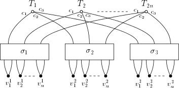
Figure 1: Rank $d=3$ orthogonal tensor contractions.

We shall focus on $d=3$. The general case $d$ will follow from this case. We denote $S_{2n}$ the symmetric group of order $(2n)!$. Counting possible graphs consists of enumerating the triples

$$(\sigma_{1},\sigma_{2},\sigma_{3})\in S_{2n}\times S_{2n}\times S_{2n}$$ (9)

subjected to the equivalence

$$(\sigma_{1},\sigma_{2},\sigma_{3})\sim(\gamma_{1}\sigma_{1}\gamma,\gamma_{2}\sigma_{2}\gamma,\gamma_{3}\sigma_{3}\gamma)\,,$$ (10)

where $\gamma\in S_{2n}$ and the $\gamma_{i}$ belong to the so-called wreath product subgroup $\in S_{n}[S_{2}]\subset S_{2n}$. We intend to count the points in the double coset

$$(S_{n}[S_{2}]\times S_{n}[S_{2}]\times S_{n}[S_{2}]){\setminus}(S_{2n}\times S_{2n}\times S_{2n})/{\rm Diag}(S_{2n})\,.$$ (11)

Let us denote $Z_{3}(2n)$ the cardinality of this double coset.

In a broader setting [42], for two subgroups $H_{1}\subset G$ and $H_{2}\subset G$, the cardinality of the double coset $|H_{1}{\setminus}G/H_{2}|$ is given by

$$|H_{1}{\setminus}G/H_{2}|={1\over|H_{1}||H_{2}|}\sum_{C}Z_{C}^{H_{1}\rightarrow G}Z^{H_{2}\rightarrow G}_{C}\,{\rm Sym}(C)\,.$$ (12)

The sum is over conjugacy classes of $G$, and $Z_{C}^{H\rightarrow G}$ is the number of elements of $H$ in the conjugacy class $C$ of $G$.

The conjugacy classes of $S_{2n}\times S_{2n}\times S_{2n}$ are determined by triples $(p_{1},p_{2},p_{3})$, where each $p_{i}$ is a partition of $2n$. The presence of the subgroup ${\rm Diag}(S_{2n})$ implies that only conjugacy classes determined by a triple $(p,p,p)$ should be conserved in the above sum.

Applying (12), we get

$$Z_{3}(2n) = {1\over{[n!(2!)^{n}]^{3}(2n)!}}\sum_{p\,\vdash 2n}Z_{(p,p,p)}^{(S_{n}[S_{2}])^{\times 3}\to(S_{2n})^{\times 3}}\times\Big{(}{(2n)!\over{\rm Sym}(p)}\Big{)}({\rm Sym}(p))^{3}$$ (13)

$$= {1\over{[n!(2!)^{n}]^{3}}}\sum_{p\,\vdash 2n}Z_{(p,p,p)}^{(S_{n}[S_{2}])^{\times 3}\to(S_{2n})^{\times 3}}\times({\rm Sym}(p))^{2}$$ (15)

with $${\rm Sym}(p):=\prod_{i=1}^{n}(i^{p_{i}})(p_{i}!)\,,$$ (17)

and where the sum over $p=(p_{\ell})_{\ell}$ is performed over all partitions of $2n=\sum_{i}ip_{i}$. The cardinality of a conjugacy class $T_{p}$ of $S_{2n}$ with cycle structure determined by a partition $p$ is given by $|T_{p}|=(2n)!/{\rm Sym}(p)$. Next, we must determine the size of $Z_{(p,p,p)}^{(S_{n}[S_{2}])^{\times 3}\to(S_{2n})^{\times 3}}$ which is

$$Z_{(p,p,p)}^{(S_{n}[S_{2}])^{\times 3}\to(S_{2n})^{\times 3}}=(Z_{p}^{S_{n}[S_{2}]\to S_{2n}})^{3}\,.$$ (18)

We can get a single factor in this product as

$${1\over{n!(2!)^{n}}}Z_{p}^{S_{n}[S_{2}]\to S_{2n}}=\hbox{Coefficient }[\mathcal{Z}_{2}^{S_{\infty}[S_{2}]}(t,\vec{x}),t^{n}x_{1}^{p_{1}}x_{2}^{p_{2}}\dots x_{2n}^{p_{2n}}]\,,$$ (19)

where appears the generating function of the number of wreath product elements in a certain conjugacy class $p\vdash 2n$, namely

$$\mathcal{Z}_{d}^{S_{\infty}[S_{d}]}(t,\vec{x})=\sum_{n}t^{n}Z^{S_{n}[S_{d}]}(\vec{x})=e^{\sum_{i=1}^{\infty}\,\frac{t^{i}}{i}\,\Big{[}\sum_{q\vdash d}\prod_{\ell=1}^{d}\big{(}\frac{x_{i\ell}}{\ell}\big{)}^{\nu_{\ell}}\frac{1}{\nu_{\ell}!}\Big{]}}\,,$$ (20)

where $\vec{x}=(x_{1},x_{2},\dots)$, and $q=(\nu_{\ell})_{\ell}$ is a partition of $d$, such that $\sum_{\ell}\ell\nu_{\ell}=d$.

The expression (13) finally computes to

$$Z_{3}(2n)=\sum_{p\,\vdash 2n}\big{(}\hbox{Coefficient }[\mathcal{Z}_{2}^{S_{\infty}[S_{2}]}(t,\vec{x}),t^{n}x_{1}^{p_{1}}x_{2}^{p_{2}}\dots x_{2n}^{p_{2n}}]\big{)}^{3}({\rm Sym}(p))^{2}\,.$$ (21)

In general, for arbirtrary $d$, the above calculation is straightforward and yields, for any $d\geq 2$,

$$Z_{d}(2n)=\sum_{p\,\vdash 2n}\big{(}\hbox{Coefficient }[\mathcal{Z}_{2}^{S_{\infty}[S_{2}]}(t,\vec{x}),t^{n}x_{1}^{p_{1}}x_{2}^{p_{2}}\dots x_{2n}^{p_{2n}}]\big{)}^{d}({\rm Sym}(p))^{d-1}\,.$$ (22)

We can generate the sequences $Z_{3}(2n)$ and $Z_{4}(2n)$ (both with $n=1,\cdots,10$) using a Mathematica program in Appendix B and obtain, respectively,

$$1,5,16,86,448,3580,34981,448628,6854130,121173330$$ (23)

and

$$1,14,132,4154,234004,24791668,3844630928,809199787472,$$ (24)

$$220685007519070,75649235368772418\,.$$ (25)

Following Read [42], the number $Z_{d}(2n)$ of $d$-regular colored graphs made with $2n$ vertices is the coefficient of $t^{n}$ in $\prod_{m}\Phi_{m}(t)$, with $m$ sufficiently large to collect all such coefficients, and where

$$\Phi_{m}(t)=\left\{\begin{array}[]{rl}\sum_{j=0}^{\infty}\frac{(A_{m/2}(j))^{d}}{j!m^{j}}t^{mj/2}&\mbox{ if }k=1,\\ \\ \sum_{j=0}^{\infty}\frac{(2j)^{d-1}}{j!^{d}}\big{(}\frac{m^{d-2}}{2^{k}}\big{)}^{j}t^{mj}&\mbox{ if }m\mbox{ is odd},\end{array}\right.$$ (29)

and the function $A_{k}(j)$ is related to the $j$-th Hermite polynomial by $A_{k}(j)=(i\sqrt{k})^{j}H_{j}(\frac{1}{2i\sqrt{k}})$.

We generate the corresponding sequences $Z_{3}(2n)$, $n=1,\cdots,10$, and $Z_{4}(2n)$, $n=1,\cdots,10$, using a Mathematica program (in Appendix B) and the results match with (23) and (24), respectively. Hence, both methods yield the same results. The sequence (23) naturally corresponds to the OEIS sequence A002830 (number of 3-regular edge colored graphs with $2n$ nodes) [43]. The sequence (24) is not yet reported on the OEIS. Hence, the formula (22) generates arbitrary new sequences for each $d>3$.

We must underline that the above counting of observables concerns connected and disconnected graphs (generalized multi-matrix invariants). To obtain only connnected invariants, we use the plethystic logarithm (Plog) transform on the generating series of the disconnected invariants. Such a generating function also easily programs with the Möbius $\mu$-function. We obtain the enumeration of connected invariants (see Appendix B) for rank $d=3$ and $4$, respectively, up to order $n=10$ as,

$$1,4,11,60,318,2806,29359,396196,6231794,112137138\,,$$ (30)

and

$$1,13,118,3931,228316,24499085,3816396556,805001547991,219822379032704,$$ (31)

$$75417509926065404\,.$$ (32)

As an illustration, Figure 2 depicts the rank 3 connected orthogonal invariants up to valence 6. The colors $c_{i}=1,2,3$, should be permuted to generate the full set of connected invariants.

Figure 2: Connected colored graphs associated with rank 3 orthogonal tensor invariants with up to 6 vertices.

3.2 TFT formulation

From the above symmetric group formulation of the counting of tensor invariants, one extracts more information via other correspondences. In particular, the enumeration reformulates as a partition function of a Topological Field Theory on a 2-complex (in short TFT₂) with $S_{2n}$ and its subgroup $S_{n}[S_{2}]$ as gauge groups. For a review of TFT’s, see [44, 45] and, in notation closer to what we aim at, see [26, 25].

Consider the counting of classes in the double coset (11), denote it as $Z_{3}(2n)$, and then consider the relation (12). Using Burnside’s lemma, we have in standard notations:

$$Z_{3}(2n)={1\over{[n!(2!)^{n}]^{3}(2n)!}}\sum_{\gamma_{i}\in S_{n}[S_{2}]}\sum_{\sigma_{i}\in S_{2n}}\sum_{\gamma\in S_{2n}}\delta(\gamma_{1}\sigma_{1}\gamma\sigma_{1}^{-1})\delta(\gamma_{2}\sigma_{2}\gamma\sigma_{2}^{-1})\delta(\gamma_{3}\sigma_{3}\gamma\sigma_{3}^{-1})\,,$$ (33)

where $\delta$ is the Kronecker symbol on $S_{2n}$. This counting interprets as a partition function of a TFT₂ on a cellular complex given by Figure 3. On that lattice, we use two gauge groups $S_{2n}$ and $S_{n}[S_{2}]$. The topology of that 2-complex is that of three cylinders sharing the same end circle. Thus, enumerating orthogonal invariant corresponds to a $S_{2n}$–TFT₂ on 3 glued cylinders along one circle, with a restriction of the gauge group to be $S_{n}[S_{2}]$ at the opposite boundary circle. This TFT₂ has boundary holonomies endowed with $S_{n}[S_{2}]$ group elements.

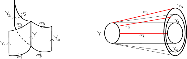
Figure 3: TFT₂ associated with the counting of orthogonal invariants.

By successively integrating some delta functions, the TFT₂ formulation produces alternative interpretations of the same counting. We extract $\gamma$ from (33) and get $\gamma=\sigma_{3}^{-1}\gamma^{-1}_{3}\sigma_{3}$ such that

$$Z_{3}(2n)={1\over{[n!(2!)^{n}]^{3}(2n)!}}\sum_{\gamma_{i}\in S_{n}[S_{2}]}\sum_{\sigma_{i}\in S_{2n}} \delta(\gamma_{1}\sigma_{1}(\sigma_{3}^{-1}\gamma^{-1}_{3}\sigma_{3})\sigma_{1}^{-1})\times$$ (35)

$$\delta(\gamma_{2}\sigma_{2}(\sigma_{3}^{-1}\gamma^{-1}_{3}\sigma_{3})\sigma_{2}^{-1})\,.$$

A change of variables $\sigma_{1,2}\to\sigma_{1,2}\sigma_{3}^{-1}$ leads us to

$$Z_{3}(2n)={1\over{[n!(2!)^{n}]^{3}}}\sum_{\gamma_{i}\in S_{n}[S_{2}]}\sum_{\sigma_{1,2}\in S_{2n}}\delta(\gamma_{1}\sigma_{1}\gamma_{3}\sigma_{1}^{-1})\delta(\gamma_{2}\sigma_{2}\gamma_{3}\sigma_{2}^{-1})\,.$$ (36)

This integration illustrates, in Figure 4, as the removal of a 1-cell associated with the variable $\gamma$ in the 2-complex. The partition function therefore shows two types of invariances: the extraction of $\gamma$ corresponds to one type of topological invariance, and then, it is followed by the change of variables $\sigma_{1,2}\to\sigma_{1,2}\sigma_{3}^{-1}$ corresponding to a topological invariance of a second kind.

Figure 4: Topological transformations of the 2-complex leaving the partition function stable.

Thus, the partition function (36) can also be written as

$$Z_{3}(2n)=Z(S^{1}\times I;(D_{S_{n}[S_{2}]})^{\times 3})\,,$$ (37)

where $Z(S^{1}\times I;(D_{S_{n}[S_{2}]})^{\times 3})$ is the partition function obtained by inserting 3 $S_{n}[S_{2}]$-defects, one at each end of the cylinder $S^{1}\times I$, and another one at finite time $t_{0}\in I$, see Figure 5. A defect defines as a closed non-intersecting loop with a marked point. The relation (37) shows that orthogonal invariants are in one-to-one correspondence with $n$-fold covers of the cylinder with 3 defects, up to a (symmetry) factor, the stabilizer subgroup of the graph that we denote ${\rm Aut}(G_{\sigma_{1},\sigma_{2},\sigma_{3}})$.

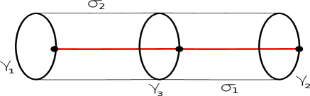
Figure 5: Cylinder with 3 defects.

The order of the stabilizer infers from

$${\rm Sym}(\sigma_{1},\sigma_{2})=\sum_{\gamma_{i}\in S_{n}[S_{2}]}\delta(\gamma_{1}\sigma_{1}\gamma_{3}\sigma_{1}^{-1})\delta(\gamma_{2}\sigma_{2}\gamma_{3}\sigma_{2}^{-1})={\rm Aut}(G_{\sigma_{1},\sigma_{2},\sigma_{3}})$$ (38)

which also relates to the number of equivalences $(S_{n}[S_{2}]\times S_{n}[S_{2}]){\setminus}(S_{n}\times S_{n})/{\rm Diag}(S_{n}[S_{2}])$ corresponding to a fixed $(\sigma_{1},\sigma_{2})$.

The TFT formulation of the counting could enrich it with a geometrical picture. Most of the time, the base space of the TFT is viewed as a string worldsheet. The counting becomes now counting of worldsheet maps over a cylinder with defects. As noticed elsewhere [20, 35], this once again shows that a link may exist between tensor models and string theory, which could be elucidated via the TFT formalism. Such link may be worth investigating in the future.

Rank $d$ counting and TFT₂ – More generally, for rank $d\geq 3$, the counting $Z_{d}(2n)$ has a TFT₂ formulation that generalizes what we discuss above in a straightforward manner:

$$Z_{d}(2n) = {1\over{[n!(2!)^{n}]^{d}(2n)!}}\sum_{\gamma_{i}\in S_{n}[S_{2}]}\sum_{\sigma_{i}\in S_{2n}}\sum_{\gamma\in S_{2n}}\prod_{i=1}^{d}\delta(\gamma_{i}\sigma_{i}\gamma\sigma_{i}^{-1})$$ (39)

$$= {1\over{[n!(2!)^{n}]^{d}}}\sum_{\gamma_{i}\in S_{n}[S_{2}]}\sum_{\sigma_{i}\in S_{2n}}\prod_{i=1}^{d-1}\delta(\gamma_{i}\sigma_{i}\gamma_{d}\sigma_{i}^{-1})\,.$$ (40)

The first equation of (39) shows that, in rank $d$, the TFT₂-formulation of the counting extends Figure 3 as the gluing of $d$ cylinders along one circle. After integration, the second equations reveals that the counting orthogonal invariants amounts therefore counting of weighted covers of $d-1$ cylinders with $d$ defects, with one of the defects shared by all cylinders. In formula, we have $Z_{d}(2n)=Z(S^{1}\times I;(D_{S_{n}[S_{2}]})^{\times d})$.

3.3 The counting as a Kronecker sum

We now revisit the counting (33) under a different light, that of the representation theory of the symmetric group (Appendix A reviews the main identities used in this section and the following). Irreducible representations (irreps) of the symmetric group $S_{2n}$ are labeled by partitions $R\vdash 2n$, that are also Young diagrams.

Starting from the Burnside lemma formulation of the counting (33), consider the following expansion of the counting of rank 3 invariants using the representation theory of $S_{2n}$:

$$Z_{3}(2n)=\frac{1}{[n!(2!)^{n}]^{3}(2n)!}\sum_{\gamma_{l}\in S_{n}[S_{2}]}\sum_{\sigma_{l}\in S_{2n}}\sum_{\gamma\in S_{2n}}\delta(\gamma_{1}\sigma_{1}\gamma\sigma_{1}^{-1})\delta(\gamma_{2}\sigma_{2}\gamma\sigma_{2}^{-1})\delta(\gamma_{3}\sigma_{3}\gamma\sigma_{3}^{-1})$$ (41)

(42)

$$=\frac{1}{[n!(2!)^{n}]^{3}(2n)!}\sum_{\gamma_{l}\in S_{n}[S_{2}]}\sum_{\gamma\in S_{2n}}\sum_{R_{l}\,\vdash\,2n}\chi^{R_{1}}(\gamma_{1})\chi^{R_{1}}(\gamma)\chi^{R_{2}}(\gamma_{2})\chi^{R_{2}}(\gamma)\chi^{R_{3}}(\gamma_{3})\chi^{R_{3}}(\gamma)$$ (43)

$$=\frac{1}{[n!(2!)^{n}]^{3}}\sum_{R_{l}\,\vdash\,2n}\textbf{C}(R_{1},R_{2},R_{3})\Big{[}\sum_{\gamma_{1}\in S_{n}[S_{2}]}\chi^{R_{1}}(\gamma_{1})\Big{]}\Big{[}\sum_{\gamma_{2}\in S_{n}[S_{2}]}\chi^{R_{2}}(\gamma_{2})\Big{]}$$ (44)

where $\chi^{R}(\cdot)$ denotes the character in the representation $R$; we used the identity (A.4) in Appendix A.1 to compute the delta’s, and the Kronecker coefficient is defined as

$$\textbf{C}(R_{1},R_{2},R_{3})=\frac{1}{2n!}\sum_{\gamma\in S_{2n}}\chi^{R_{1}}(\gamma)\chi^{R_{2}}(\gamma)\chi^{R_{3}}(\gamma)\,.$$ (45)

The Kronecker defines the multiplicity of the representation $R_{3}$ in the tensor product $R_{1}\otimes R_{2}$, or the multiplicity of the trivial representation in $R_{1}\otimes R_{2}\otimes R_{3}$ when expanded back in irreps.

Above, the sums over the subgroup $S_{n}[S_{2}]$ have been not yet performed. To proceed with these sums, we will use a useful result by Howe [46] (see also a result by Mizukawa, proposition 4.1 in [47], and also [48, 49] or a more recent use of it in [30]):

$$\sum_{\gamma\in S_{n}[S_{2}]}\chi^{R}(\gamma)=|S_{n}[S_{2}]|\,m^{R}$$ (46)

where $m^{R}=1$ if $R$ is an “even” partition, that is, all its row lengths are even, and $m^{R}=0$ otherwise. This result is derived from a more general formula $\sum_{\gamma\in S_{n}[S_{2}]}\chi^{A}(\gamma)\chi^{R}(\gamma)=|S_{n}[S_{2}]|\,m^{A|R}$, where $A$ is an irreps of $S_{n}[S_{2}]$ subduced by $R$ irreps of $S_{2n}$, and then inserting $A$ as the trivial representation $\overline{[2n]}$ of $S_{n}[S_{2}]$.

Then, we obtain, inserting this in (41)

$$Z_{3}(2n)=\sum_{R_{l}\,\vdash\,2n/R_{l}\text{ is even }}\textbf{C}(R_{1},R_{2},R_{3})\,.$$ (47)

Comparing this sequence and (23), we produce a Sage code (see Appendix B) showing that the numbers generated by (47) match with (23).

In the next section, we will show that, this number is also the dimension of an algebra $\mathcal{K}_{3}(n)$. It is an interesting problem to investigate how the counting of colored graphs could contribute to the famous problem of giving a combinatorial interpretation to the Kronecker coefficients [39, 40] (in the same way that Littlewood-Richardson coefficient have found a combinatorial description). From previous work [35], we know that the sum of squares of Kronecker coefficients associated with $S_{n}$ equals the number of $d$-regular bipartite colored graphs made with $n$ black and $n$ white vertices. Here the interpretation is the following, the number of $d$-regular colored graphs (not necessarily bipartite) equals the sum of all Kronecker’s precluded those that are defined with partitions with odd rows. An idea to contribute to the above problem is to refine the counting of graphs in a way to boil down to a single Kronecker coefficient. In other words, given a non vanishing Kronecker coefficient is it possible to list all graphs contributing to that Kronecker coefficient? This is certainly a difficult problem that will require new tools in representation theory.

Counting rank-$d$ tensor invariants - The above counting generalize quite naturally at any rank $d$ as

$$Z_{d}(2n) =\frac{1}{[n!(2!)^{n}]^{d}(2n)!}\sum_{\gamma_{l}\in S_{n}[S_{2}]}\sum_{\sigma_{l}\in S_{2n}}\sum_{\gamma\in S_{2n}}\prod_{i=1}^{d}\delta(\gamma_{i}\sigma_{i}\gamma\sigma_{i}^{-1})$$ (48)

$$=\frac{1}{[n!(2!)^{n}]^{d}}\sum_{R_{l}\,\vdash\,2n}\sum_{\gamma_{l}\in S_{n}[S_{2}]}\textbf{C}_{d}(R_{1},\ldots,R_{d})\chi^{R_{1}}(\gamma_{1})\ldots\chi^{R_{d}}(\gamma_{d})$$

$$=\sum_{R_{l}\,\vdash\,2n/R_{l}\text{ is even }}\sum_{\gamma_{l}\in S_{n}[S_{2}]}\textbf{C}_{d}(R_{1},\ldots,R_{d})$$

where we introduced the notation

$$\textbf{C}_{k}(R_{1},\ldots,R_{k})=\frac{1}{(2n)!}\sum_{\gamma\in S_{2n}}\chi^{R_{1}}(\gamma)\ldots\chi^{R_{k}}(\gamma)\,.$$ (49)

This counts the multiplicity of the one dimensional trivial $S_{2n}$ irrep in the tensor product of irreps $R_{1}\otimes\ldots\otimes R_{k}$. It expresses as a convoluted product of Kronecker coefficients as

$$\textbf{C}_{k}(R_{1},\ldots,R_{k})=\sum_{S_{l}\vdash 2n}\textbf{C}(R_{1},R_{2},S_{1})\left[\prod_{i=1}^{k-4}\textbf{C}(S_{i},R_{i+2},S_{i+1})\right]\textbf{C}(S_{k-3},R_{k-1},R_{k})\,.$$ (50)

4 Double coset algebra

We now discuss the underlying structure, an algebra, determined by the counting of the $O(N)$ invariants. The rank 3 case is first addressed for the sake of simplicity, and from that, we will infer the general rank-$d$ case whenever possible.

Consider $\mathbb{C}[S_{2n}]$, the group algebra of $S_{2n}$. Our construction depends on tensor products of that space.

$\mathcal{K}_{d}(2n)$ as a double coset algebra in $\mathbb{C}[S_{2n}]^{\otimes d}$ - We fix $d=3$. Consider $\sigma_{1}\otimes\sigma_{2}\otimes\sigma_{3}$ as an element of the group algebra $\mathbb{C}[S_{2n}]^{\otimes 3}$, and three left actions of the subgroup $S_{n}[S_{2}]$ and the diagonal right action ${\rm Diag}(\mathbb{C}(S_{2n}))$ on this triple as:

$$\sigma_{1}\otimes\sigma_{2}\otimes\sigma_{3}\rightarrow\sum_{\gamma_{i}\in S_{n}[S_{2}]}\sum_{\gamma\in S_{2n}}\gamma_{1}\sigma_{1}\gamma\otimes\gamma_{2}\sigma_{2}\gamma\otimes\gamma_{3}\sigma_{3}\gamma\,.$$ (51)

$\mathcal{K}_{3}(2n)$ is the vector subspace of $\mathbb{C}[S_{2n}]^{\otimes 3}$ which is invariant under these subgroup actions:

$$\mathcal{K}_{3}(2n)=\text{Span}_{\mathbb{C}}\left\{\sum_{\gamma_{i}\in S_{n}[S_{2}]}\sum_{\gamma\in S_{2n}}\gamma_{1}\sigma_{1}\gamma\otimes\gamma_{2}\sigma_{2}\gamma\otimes\gamma_{3}\sigma_{3}\gamma,\quad\sigma_{1},\sigma_{2},\sigma_{3}\in S_{2n}\right\}$$ (52)

It is obvious that $\dim\mathcal{K}_{3}(2n)=Z_{3}(2n)$, since each base element represents the graph equivalent class counted once in $Z_{3}(2n)$. Pick two base elements, called henceforth graph base elements, and consider their product

$$\Big{[}\sum_{\gamma_{i}\in S_{n}[S_{2}]}\sum_{\gamma\in S_{2n}}\gamma_{1}\sigma_{1}\gamma\otimes\gamma_{2}\sigma_{2}\gamma\otimes\gamma_{3}\sigma_{3}\gamma\Big{]}\Big{[}\sum_{\tau_{i}\in S_{n}[S_{2}]}\sum_{\tau\in S_{2n}}\tau_{1}\sigma^{\prime}_{1}\tau\otimes\tau_{2}\sigma^{\prime}_{2}\tau\otimes\tau_{3}\sigma_{3}^{\prime}\tau\Big{]}$$ (53)

(54)

$$=\sum_{\gamma_{i},\tau_{i}\in S_{n}[S_{2}]}\sum_{\gamma,\tau\in S_{2n}}\gamma_{1}\sigma_{1}\gamma\tau_{1}\sigma^{\prime}_{1}\tau\otimes\gamma_{2}\sigma_{2}\gamma\tau_{2}\sigma^{\prime}_{2}\tau\otimes\gamma_{3}\sigma_{3}\gamma\tau_{3}\sigma_{3}^{\prime}\tau$$ (55)

(56)

$$=\sum_{\tau_{i}\in S_{n}[S_{2}]}\sum_{\gamma\in S_{2n}}\Big{[}\sum_{\gamma_{i}\in S_{n}[S_{2}]}\sum_{\tau\in S_{2n}}\gamma_{1}(\sigma_{1}\gamma\tau_{1}\sigma^{\prime}_{1})\tau\otimes\gamma_{2}(\sigma_{2}\gamma\tau_{2}\sigma^{\prime}_{2})\tau\otimes\gamma_{3}(\sigma_{3}\gamma\tau_{3}\sigma_{3}^{\prime})\tau\Big{]}$$ (57)

This shows that the multiplication remains in the vector space. Hence, $\mathcal{K}_{3}(2n)$ is an algebra and (53) defines a graph multiplication. The proof is totally similar for $\mathcal{K}_{d}(2n)$ (considering $d$ factors in the tensor product) which is thus an algebra of dimension $Z_{d}(2n)$.

The product of graphs in the algebra $\mathcal{K}_{3}(2n)$ illustrates as in Figure 6.

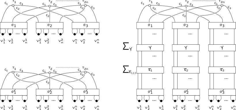
Figure 6: Product of two graph base elements (on the left) gives a sum of graphs (on the right).

Gauge fixing - There is a gauge fixing procedure in the construction of orthogonal invariants. One initially fixes a permutation $\sigma_{i}$ but is still able to generate all invariants. Consider $\xi=(12)(34)\dots(2n-1,2n)$, and we fix $\sigma_{1}$ to belong to the stabilizer of $\xi$, i.e. $\sigma_{1}^{-1}\xi\sigma_{1}=\xi$. Since the Stab${}_{\xi}=S_{n}[S_{2}]$, we simply mean that we choose $\sigma_{1}$ to be in that subgroup. We already observe a difference with the unitary case [35]. Indeed, while the gauge fixing in the unitary case leads to the definition of a permutation centralizer algebra, the gauge fixing here will not bring such an algebra. The main difference with the unitary case also rests on the fact that the left and right invariances on the triple $(\sigma_{1},\sigma_{2},\sigma_{3})$ in this case are radically different.

Associativity - In the graph base, we can check the associativity of the product of elements of $\mathcal{K}_{3}(2n)$:

$$\Bigg{(}\Big{[}\sum_{\gamma_{i}\in S_{n}[S_{2}]}\sum_{\gamma\in S_{2n}}\gamma_{1}\sigma_{1}\gamma\otimes\gamma_{2}\sigma_{2}\gamma\otimes\gamma_{3}\sigma_{3}\gamma\Big{]}\Big{[}\sum_{\tau_{i}\in S_{n}[S_{2}]}\sum_{\tau\in S_{2n}}\tau_{1}\sigma_{1}^{\prime}\tau\otimes\tau_{2}\sigma_{2}^{\prime}\tau\otimes\tau_{3}\sigma_{3}^{\prime}\tau\Big{]}\Bigg{)}$$ (58)

$$\times\Big{[}\sum_{\alpha_{i}\in S_{n}[S_{2}]}\sum_{\alpha\in S_{2n}}\alpha_{1}\sigma_{1}^{\prime\prime}\alpha\otimes\alpha_{2}\sigma_{2}^{\prime\prime}\alpha\otimes\alpha_{3}\sigma_{3}^{\prime\prime}\alpha\Big{]}$$ (59)

$$=\sum_{\tau_{i},\,\alpha_{i}}\sum_{\gamma,\,\tau}\Big{[}\sum_{\gamma,\alpha}\gamma_{1}\sigma_{1}\gamma\tau_{1}\sigma_{1}^{\prime}\tau\alpha_{1}\sigma_{1}^{\prime\prime}\alpha\otimes\gamma_{2}\sigma_{2}\gamma\tau_{2}\sigma_{2}^{\prime}\tau\alpha_{2}\sigma_{2}^{\prime\prime}\alpha\otimes\gamma_{3}\sigma_{3}\gamma\tau_{3}\sigma_{3}^{\prime}\tau\alpha_{3}\sigma_{3}^{\prime\prime}\alpha\Big{]}$$ (60)

$$=\Big{[}\sum_{\gamma_{i}\in S_{n}[S_{2}]}\sum_{\gamma\in S_{2n}}\gamma_{1}\sigma_{1}\gamma\otimes\gamma_{2}\sigma_{2}\gamma\otimes\gamma_{3}\sigma_{3}\gamma\Big{]}$$ (61)

$$\times\left(\Big{[}\sum_{\tau_{i}\in S_{n}[S_{2}]}\sum_{\tau\in S_{2n}}\tau_{1}\sigma_{1}^{\prime}\tau\otimes\tau_{2}\sigma_{2}^{\prime}\tau\otimes\tau_{3}\sigma_{3}^{\prime}\tau\Big{]}\Big{[}\sum_{\alpha_{i}\in S_{n}[S_{2}]}\sum_{\alpha\in S_{2n}}\alpha_{1}\sigma_{1}^{\prime\prime}\alpha\otimes\alpha_{2}\sigma_{2}^{\prime\prime}\alpha\otimes\alpha_{3}\sigma_{3}^{\prime\prime}\alpha\Big{]}\right)$$ (62)

The proof easily extends to any $d$, and we therefore claim the following:

Proposition 4.1

$\mathcal{K}_{d}(2n)$ is an associative unital sub-algebra of $\mathbb{C}[S_{2n}]^{\otimes 3}$.

The unity is given by the equivalence class of $(id,id,id)$. Such element corresponds to the disconnected graph made with $n$ connected components with full contraction of $n$ pairs of tensors.

Pairing - There is an inner product (that we will call pairing) on $\mathcal{K}_{d}(2n)$ defined from the linear extension of the delta function from the symmetric group to the tensor product group algebra (see (A.28) in Appendix A.3 for details pertaining to the following notation). Take two base elements (in obvious notation) and evaluate using proper change of variables:

$${\boldsymbol{\delta}}\Big{(}\sum_{\gamma_{i},\gamma}\otimes_{i}^{d}\gamma_{i}\sigma_{i}\gamma;\sum_{\tau_{i},\tau}\otimes_{i}^{d}\tau_{i}\sigma^{\prime}_{i}\tau\Big{)}=\sum_{\gamma_{i},\gamma}\sum_{\tau_{i},\tau}\prod_{i}^{d}\delta(\gamma_{i}\sigma_{i}\gamma(\tau_{i}\sigma^{\prime}_{i}\tau)^{-1})$$ (64)

$$=[(2n)!(n!2^{n})]\sum_{\gamma_{i},\gamma}\prod_{i}^{d}\delta(\gamma_{i}\sigma_{i}\gamma(\sigma^{\prime}_{i})^{-1})\,.$$ (65)

Thus, either the tuples $(\sigma_{1},\sigma_{2},\dots,\sigma_{d})$ and $(\sigma^{\prime}_{1},\sigma^{\prime}_{2},\dots,\sigma^{\prime}_{d})$ define equivalent graphs $G_{\sigma_{1},\sigma_{2},\dots,\sigma_{d}}$ and $G_{\sigma^{\prime}_{1},\sigma^{\prime}_{2},\dots,\sigma^{\prime}_{d}}$, respectively, or the result is 0. This precisely tells us that the graph base forms an orthogonal system. The above computes further using the order of the automorphism group of the graph

$${\boldsymbol{\delta}}\Big{(}\sum_{\gamma_{i},\gamma}\otimes_{i}^{d}\gamma_{i}\sigma_{i}\gamma;\sum_{\tau_{i},\tau}\otimes_{i}^{d}\tau_{i}\sigma^{\prime}_{i}\tau\Big{)}=[(2n)!(n!2^{n})]\delta(G_{\sigma_{1},\sigma_{2},\dots,\sigma_{d}};G_{\sigma^{\prime}_{1},\sigma^{\prime}_{2},\dots,\sigma^{\prime}_{d}}){\rm Aut}(G_{\sigma_{1},\sigma_{2},\dots,\sigma_{d}})\,.$$ (66)

Therefore, there exists a non degenerate bilinear pairing on $\mathcal{K}_{d}(2n)$ and the following holds:

Theorem 4.2

$\mathcal{K}_{d}(2n)$ is an associative unital semi-simple algebra.

As a corollary of Theorem 4.2, the Wedderburn-Artin theorem guarantees that $\mathcal{K}_{d}(2n)$ decomposes in matrix subalgebras. It might be interesting to investigate a base of such a decomposition of $\mathcal{K}_{d}(2n)$ in irreducible matrix subalgebras. One could be tempted to think that, at $d=3$, restricting to $\mathcal{K}_{3}(2n)$, the Kronecker coefficients for even partitions could be themselves squares, and therefore define the dimensions of the irreducible subalgebras. This is not the case as this can be easily shown using the same Sage code given in Appendix B (by printing the Kronecker). This point is postponed for future investigations. In the mean time, it is legitimate to ask a representation base with labels that reflect the dimension (47). This is the purpose of the next paragraph.

Constructing a representation theoretic base $Q$ of $\mathcal{K}_{3}(2n)$ - Let us introduce the representation base of $\mathbb{C}[S_{2n}]$ given by the elements

$$Q^{R}_{ij}=\frac{\kappa_{R}}{(2n)!}\sum_{\sigma\in S_{2n}}D^{R}_{ij}(\sigma)\sigma\,,\qquad\text{with}\;\kappa_{R}^{2}=(2n)!d(R)\,,$$ (67)

that obey the orthogonality relation $\delta(Q^{R}_{ij};Q^{R^{\prime}}_{i^{\prime}j^{\prime}})=\delta_{RR^{\prime}}\delta_{ii^{\prime}}\delta_{jj^{\prime}}$. The base $\{Q^{R}_{ij}\}$ counts $\sum_{R\vdash 2n}(d(R))^{2}=(2n)!$ elements and forms the Fourier theoretic base of ${\mathbb{C}}[S_{2n}]$. Appendix A.3 collects a few other properties of this base for a general permutation group.

We fix $d=3$ and build now the invariant representation theoretic (Fourier for short) base of the algebra $\mathcal{K}_{3}(2n)$ (52). Consider the right diagonal action $\rho_{R}(\cdot)$ and the three left actions $\varrho_{i}(\cdot)$ on the tensor product $\mathbb{C}[S_{2n}]^{\otimes 3}$. Then we write:

$$\sum_{\begin{subarray}{c}\gamma_{1},\,\gamma_{2},\,\gamma_{3}\in S_{n}[S_{2}]\end{subarray}}\sum_{\gamma\in S_{2n}}\varrho_{1}(\gamma_{1})\varrho_{2}(\gamma_{2})\varrho_{3}(\gamma_{3})\rho_{R}(\gamma)\,Q^{R_{1}}_{i_{1}j_{1}}\otimes Q^{R_{2}}_{i_{2}j_{2}}\otimes Q^{R_{3}}_{i_{3}j_{3}}$$ (68)

$$=\sum_{\gamma_{a}}\sum_{\gamma}\gamma_{1}\,Q^{R_{1}}_{i_{1}j_{1}}\gamma\otimes\gamma_{2}\,Q^{R_{2}}_{i_{2}j_{2}}\,\gamma\otimes\gamma_{3}\,Q^{R_{3}}_{i_{3}j_{3}}\,\gamma$$

$$=\sum_{\gamma_{a}}\sum_{\gamma}\sum_{p_{l}\,,q_{l}}D^{R_{1}}_{p_{1}i_{1}}(\gamma_{1})Q^{R_{1}}_{p_{1}q_{1}}D^{R_{1}}_{j_{1}q_{1}}(\gamma)\otimes D^{R_{2}}_{p_{2}i_{2}}(\gamma_{2})Q^{R_{2}}_{p_{2}q_{2}}D^{R_{2}}_{j_{2}q_{2}}(\gamma)\otimes D^{R_{3}}_{p_{3}i_{3}}(\gamma_{3})Q^{R_{3}}_{p_{3}q_{3}}D^{R_{3}}_{j_{3}q_{3}}(\gamma)$$

$$=\frac{(2n)!}{d(R_{3})}\sum_{\gamma_{a}}\sum_{p_{l}\,,q_{l}}\sum_{\tau}C^{R_{1},R_{2};R_{3},\tau}_{j_{1},j_{2};j_{3}}C^{R_{1},R_{2};R_{3},\tau}_{q_{1},q_{2};q_{3}}D^{R_{1}}_{p_{1}i_{1}}(\gamma_{1})D^{R_{2}}_{p_{2}i_{2}}(\gamma_{2})D^{R_{3}}_{p_{3}i_{3}}(\gamma_{3})Q^{R_{1}}_{p_{1}q_{1}}\otimes Q^{R_{2}}_{p_{2}q_{2}}\otimes Q^{R_{3}}_{p_{3}q_{3}}.$$

We used (A.26) to multiply group elements with the $Q$ base, see Appendix A.3; then use (A.19) to sum over $\gamma$ the 3 representation matrices, see in Appendix A.2.

We couple this last result with a Clebsch-Gordan coefficient, in order to get, using (A.15):

$$\sum_{j_{l}}C^{R_{1},R_{2};R_{3},\tau}_{j_{1},j_{2};j_{3}}\sum_{\gamma_{a}}\sum_{\gamma}\varrho_{1}(\gamma_{1})\varrho_{2}(\gamma_{2})\varrho_{3}(\gamma_{3})\rho_{R}(\gamma)\,Q^{R_{1}}_{i_{1}j_{1}}\otimes Q^{R_{2}}_{i_{2}j_{2}}\otimes Q^{R_{3}}_{i_{3}j_{3}}$$ (69)

$$=(2n)!\sum_{p_{l}\,,q_{l}}C^{R_{1},R_{2};R_{3},\tau}_{q_{1},q_{2};q_{3}}\sum_{\gamma_{1}}D^{R_{1}}_{p_{1}i_{1}}(\gamma_{1})\sum_{\gamma_{2}}D^{R_{2}}_{p_{2}i_{2}}(\gamma_{2})\sum_{\gamma_{3}}D^{R_{3}}_{p_{3}i_{3}}(\gamma_{3})Q^{R_{1}}_{p_{1}q_{1}}\otimes Q^{R_{2}}_{p_{2}q_{2}}\otimes Q^{R_{3}}_{p_{3}q_{3}}\,.$$

Once again, we should stress the fact that $\sum_{\gamma\in S_{n}[S_{2}]}D^{R}_{pq}(\gamma)\neq 0$, if and only if $R$ is a partition of $2n$ with even rows. This condition will be always assumed in the next calculations. Now, we can split the Wigner matrix element using branching coefficients of $S_{n}[S_{2}]$ in $S_{2n}$. Consider $V^{R}$ a irreps $S_{2n}$ (see Appendix A listing a few basic facts on representation theory of $S_{n}$ and our notations), and the subgroup inclusion $S_{n}[S_{2}]\subset S_{2n}$, we can decompose $V^{R}$ in irreps $V^{r}$ of $S_{n}[S_{2}]$ as

$$V^{R}=\oplus_{r}V^{r}\otimes V_{R,r}$$ (70)

where $V_{R,r}$ is a vector space of dimension the multiplicity of the irreps $r$ in $R$. A state in this decomposition denotes $\left|r,m_{r},\nu_{r}\right\rangle$, where $m_{r}$ labels the states of $V^{r}$ and $\nu_{r}=1,\dots,\dim V_{R,r}$.

The branching coefficients that are of interest are the coefficients of $\left|r,m_{r},\nu_{r}\right\rangle$ when decomposed in an orthonormal base of the irreps $R$:

$$B^{R;\,r,\nu_{r}}_{i;\,m_{r}}=\langle R,i\left|r,m_{r},\nu_{r}\right\rangle=\langle r,m_{r},\nu_{r}\left|R,i\right\rangle\,.$$ (71)

The last relation is deduced from the fact that we use real representations. Using the decomposition of the identity, the branching coefficients satisfy the following identities

$$\sum_{i}B^{R;\,r,\nu_{r}}_{i;\,m_{r}}B^{R;\,s,\nu_{s}}_{i;\,m_{s}}=\delta_{rs}\delta_{\nu_{r}\nu_{s}}\delta_{m_{r}m_{s}}$$ (72)

$$\sum_{r,m_{r},\nu_{r}}B^{R;\,r,\nu_{r}}_{i;\,m_{r}}B^{R^{\prime};\,r,\nu_{r}}_{i^{\prime};\,m_{r}}=\delta_{RR^{\prime}}\delta_{ii^{\prime}}\,.$$ (73)

We have the following useful relation, for $\sigma\in S_{n}[S_{2}]$,

$$\sum_{j}D^{R}_{ij}(\sigma)\,B^{R;\,r,\nu_{r}}_{j;m_{r}}=\sum_{m^{\prime}_{r}}D^{r}_{m_{r}m_{r}^{\prime}}(\sigma)\,B^{R;\,r,\nu_{r}}_{i;m^{\prime}_{r}}\,,$$ (74)

where $D^{r}_{m_{r}m_{r}^{\prime}}(\sigma)$ is the representation matrix of $\sigma$ as an element of $S_{n}[S_{2}]$. Restricting this to $r=\overline{[2n]}$, the trivial representation of $S_{n}[S_{2}]$ that is one dimensional and with multiplicity always 1 for all $R$, we obtain:

$$\sum_{j}D^{R}_{ij}(\sigma)\,B^{R;\overline{[2n]},1}_{j;1}=D^{\overline{[2n]}}_{11}(\sigma)\,B^{R;\overline{[2n]},1}_{i;1}=B^{R;\overline{[2n]},1}_{i;1}\,.$$ (75)

We now treat the sum over the representation matrices in (69). Inserting twice a complete set of states therein, we get

$$\sum_{\sigma\in S_{n}[S_{2}]}D^{R}_{ij}(\sigma)=\sum_{\sigma\in S_{n}[S_{2}]}\sum_{r,\nu_{r},m_{r};s,\nu_{s},m_{s}}B^{R;\,r,\nu_{r}}_{i;\,m_{r}}B^{R;\,s,\nu_{s}}_{j;\,m_{s}}\langle r,\nu_{r},m_{r}|\sigma|s,\nu_{s},m_{s}\rangle\,.$$ (76)

Noting that $\sum_{s\in S_{n}[S_{2}]}\sigma=\sum_{s\in S_{n}[S_{2}]}\sigma\chi^{\overline{[2n]}}(\sigma)$ is, up to the factor $1/[n!2^{n}]$, nothing but the projector onto the trivial $\overline{[2n]}$ representation of $S_{n}[S_{2}]$, the overlap computes to

$$\sum_{\sigma\in S_{n}[S_{2}]}\langle r,\nu_{r},m_{r}|\sigma|s,\nu_{s},m_{s}\rangle=(2^{n}n!)\delta_{r,\overline{[2n]}}\delta_{s,\overline{[2n]}}\delta_{1m_{r}}\delta_{1m_{s}}\delta_{1\nu_{s}}\delta_{1\nu_{r}}\,,$$ (77)

since we have

$$\sum_{\sigma\in S_{n}[S_{2}]}\sigma|s,\nu_{s},m_{s}\rangle=\sum_{\sigma\in S_{n}[S_{2}]}\chi^{\overline{[2n]}}(\sigma)\sum_{k}D^{s}_{m_{s}k}(\sigma)|s,\nu_{s},k\rangle$$ (78)

(79)

$$=\sum_{\sigma\in S_{n}[S_{2}]}D^{\overline{[2n]}}_{11}(\sigma)\sum_{k}D^{s}_{m_{s}k}(\sigma)|s,\nu_{s},k\rangle=\frac{2^{n}n!}{d(\overline{[2n]})}\sum_{k}\delta_{\overline{[2n]},s}\delta_{1m_{s}}\delta_{1\nu_{s}}\delta_{1k}|s,\nu_{s},k\rangle$$ (80)

(81)

$$=(2^{n}n!)\delta_{\overline{[2n]},s}\delta_{1m_{s}}\delta_{1\nu_{s}}|\overline{[2n]},1,1\rangle\,.$$ (82)

Hence,

$$\sum_{\sigma\in S_{n}[S_{2}]}D^{R}_{ij}(\sigma)=(2^{n}n!)B^{R;\,tr}_{i}B^{R;\,tr}_{j}\,,$$ (83)

where we have defined $B^{R;\,tr}_{i}=\langle R,i\,|\overline{[2n]},1,1\rangle$.

From the above calculation, we finally get from (69):

$$\sum_{j_{l}}C^{R_{1},R_{2};R_{3},\tau}_{j_{1},j_{2};j_{3}}\sum_{\gamma_{a}}\sum_{\gamma}\varrho_{1}(\gamma_{1})\varrho_{2}(\gamma_{2})\varrho_{3}(\gamma_{3})\rho_{R}(\gamma)\,Q^{R_{1}}_{i_{1}j_{1}}\otimes Q^{R_{2}}_{i_{2}j_{2}}\otimes Q^{R_{3}}_{i_{3}j_{3}}$$ (84)

$$=(2n)!(n!2^{n})^{3}B^{R_{1};tr}_{i_{1}}B^{R_{2};tr}_{i_{2}}B^{R_{3};tr}_{i_{3}}\sum_{p_{l}\,,q_{l}}C^{R_{1},R_{2};R_{3},\tau}_{q_{1},q_{2};q_{3}}B^{R_{1};\,tr}_{p_{1}}B^{R_{2};\,tr}_{p_{2}}B^{R_{3};\,tr}_{p_{3}}Q^{R_{1}}_{p_{1}q_{1}}\otimes Q^{R_{2}}_{p_{2}q_{2}}\otimes Q^{R_{3}}_{p_{3}q_{3}}$$

We now define an element

$$Q^{R_{1},R_{2},R_{3},\tau}=\kappa_{\vec{R}}\sum_{p_{l}\,,q_{l}}C^{R_{1},R_{2};R_{3},\tau}_{q_{1},q_{2};q_{3}}B^{R_{1};\,tr}_{p_{1}}B^{R_{2};\,tr}_{p_{2}}B^{R_{3};\,tr}_{p_{3}}Q^{R_{1}}_{p_{1}q_{1}}\otimes Q^{R_{2}}_{p_{2}q_{2}}\otimes Q^{R_{3}}_{p_{3}q_{3}}$$ (85)

(86)

$$=\kappa_{\vec{R}}\frac{\kappa_{R_{1}}\kappa_{R_{2}}\kappa_{R_{3}}}{((2n)!)^{3}}\sum_{\sigma_{i}}\sum_{p_{l}\,,q_{l}}C^{R_{1},R_{2};R_{3},\tau}_{q_{1},q_{2};q_{3}}\Big{[}\prod_{i=1}^{3}B^{R_{i};\,tr}_{p_{i}}D^{R_{i}}_{p_{i}q_{i}}(\sigma_{i})\Big{]}\sigma_{1}\otimes\sigma_{2}\otimes\sigma_{3}$$ (87)

where $\kappa_{\vec{R}}$ is a normalization constant to be fixed later and the notation $\vec{R}$ stands for $(R_{1},R_{2},R_{3})$. The set $\{Q^{R_{1},R_{2},R_{3},\tau}\}$ is of cardinality the counting of orthogonal invariants given by (47).

Invariance - Let us check that the element $Q^{R_{1},R_{2},R_{3},\tau}$ is invariant under left multiplication on each factor and diagonal right multiplication:

$$(\gamma_{1}\otimes\gamma_{2}\otimes\gamma_{3})Q^{R_{1},R_{2},R_{3},\tau}(\gamma\otimes\gamma\otimes\gamma)=\kappa_{\vec{R}}\sum_{p_{l}\,,q_{l}}C^{R_{1},R_{2};R_{3},\tau}_{q_{1},q_{2};q_{3}}B^{R_{1};\,tr}_{p_{1}}B^{R_{2};\,tr}_{p_{2}}B^{R_{3};\,tr}_{p_{3}}$$ (88)

(89)

$$\times\sum_{\ell_{1},j_{1}}D^{R_{1}}_{\ell_{1}p_{1}}(\gamma_{1})Q^{R_{1}}_{\ell_{1}j_{1}}D^{R_{1}}_{q_{1}j_{1}}(\gamma)\otimes\sum_{\ell_{2},j_{2}}D^{R_{2}}_{\ell_{2}p_{2}}(\gamma_{2})Q^{R_{2}}_{\ell_{2}j_{2}}D^{R_{2}}_{q_{2}j_{2}}(\gamma)\otimes\sum_{\ell_{3},j_{3}}D^{R_{3}}_{\ell_{3}p_{3}}(\gamma_{3})Q^{R_{3}}_{\ell_{3}j_{3}}D^{R_{3}}_{q_{3}j_{3}}(\gamma)$$ (90)

$$=\kappa_{\vec{R}}\sum_{j_{l}}C^{R_{1},R_{2};R_{3},\tau}_{j_{1},j_{2};j_{3}}\sum_{p_{l},\ell_{l}}D^{R_{1}}_{\ell_{1}p_{1}}(\gamma_{1})B^{R_{1};\,tr}_{p_{1}}D^{R_{2}}_{\ell_{2}p_{2}}(\gamma_{2})B^{R_{2};\,tr}_{p_{2}}D^{R_{3}}_{\ell_{3}p_{3}}(\gamma_{3})B^{R_{3};\,tr}_{p_{3}}\;Q^{R_{1}}_{\ell_{1}j_{1}}\otimes Q^{R_{2}}_{\ell_{2}j_{2}}\otimes Q^{R_{3}}_{\ell_{3}j_{3}}$$ (91)

$$=\kappa_{\vec{R}}\sum_{j_{l},\ell_{l}}C^{R_{1},R_{2};R_{3},\tau}_{j_{1},j_{2};j_{3}}B^{R_{1};\,tr}_{\ell_{1}}B^{R_{2};\,tr}_{\ell_{2}}B^{R_{3};\,tr}_{\ell_{3}}\;Q^{R_{1}}_{\ell_{1}j_{1}}\otimes Q^{R_{2}}_{\ell_{2}j_{2}}\otimes Q^{R_{3}}_{\ell_{3}j_{3}}=Q^{R_{1},R_{2},R_{3},\tau}\,,$$ (92)

where we used once again (A.26) and (A.15) at intermediate step and the identity (75) to get the last line.

We check a few properties of the product of elements of $\mathcal{K}_{3}(2n)$.

Product - The elements (67) of the Fourier base of $\mathbb{C}[S_{2n}]$ multiply as follows (see Appendix A.3.)

$$Q^{R}_{ij}Q^{R^{\prime}}_{kl}=\frac{\kappa_{R}}{d(R)}\delta_{RR^{\prime}}\delta_{jk}Q^{R^{\prime}}_{il}\,.$$ (93)

The definition (85) and relation (93) allow us to compute the product

$$\quad Q^{R_{1},R_{2},R_{3},\tau}Q^{R_{1}^{\prime},R_{2}^{\prime},R_{3}^{\prime},\tau^{\prime}}$$ (94)

$$=\frac{\kappa_{\vec{R}}\kappa_{\vec{R^{\prime}}}\kappa_{R_{1}}\kappa_{R_{2}}\kappa_{R_{3}}}{d(R_{1})d(R_{2})d(R_{3})}\delta_{\vec{R}\vec{R^{\prime}}}\sum_{p_{l}\,q_{l}\,a_{l}\,b_{l}}C^{R_{1},R_{2};R_{3},\tau}_{q_{1},q_{2};q_{3}}C^{R_{1}^{\prime},R_{2}^{\prime};R_{3}^{\prime},\tau^{\prime}}_{b_{1},b_{2};b_{3}}$$

$$\qquad\times B^{R_{1};\,tr}_{p_{1}}B^{R_{2};\,tr}_{p_{2}}B^{R_{3};\,tr}_{p_{3}}B^{R_{1}^{\prime};\,tr}_{a_{1}}B^{R_{2}^{\prime};\,tr}_{a_{2}}B^{R_{3}^{\prime};\,tr}_{a_{3}}Q^{R_{1}^{\prime}}_{p_{1}b_{1}}\otimes Q^{R_{2}^{\prime}}_{p_{2}b_{2}}\otimes Q^{R_{3}^{\prime}}_{p_{3}b_{3}}\delta_{q_{1}a_{1}}\delta_{q_{2}a_{2}}\delta_{q_{3}a_{3}}$$

$$=\frac{\kappa_{\vec{R}}\kappa_{R_{1}}\kappa_{R_{2}}\kappa_{R_{3}}}{d(R_{1})d(R_{2})d(R_{3})}\delta_{\vec{R}\vec{R^{\prime}}}\Big{[}\sum_{q_{l}}C^{R_{1}^{\prime},R_{2}^{\prime};R_{3}^{\prime},\tau}_{q_{1},q_{2};q_{3}}B^{R_{1}^{\prime};\,tr}_{q_{1}}B^{R_{2}^{\prime};\,tr}_{q_{2}}B^{R_{3}^{\prime};\,tr}_{q_{3}}\Big{]}Q^{R_{1}^{\prime},R_{2}^{\prime},R_{3}^{\prime},\tau^{\prime}}.$$

Hence, the product of two base elements expands in terms of $Q^{R_{1},R_{2},R_{3},\tau}$. In a compact notation, we write

$$Q^{R_{1},R_{2},R_{3},\tau}Q^{R_{1}^{\prime},R_{2}^{\prime},R_{3}^{\prime},\tau^{\prime}}=\delta_{\vec{R}\vec{R^{\prime}}}k(\vec{R^{\prime}},\tau)Q^{R_{1}^{\prime},R_{2}^{\prime},R_{3}^{\prime},\tau^{\prime}}.$$ (95)

which shows that the product is almost orthogonal. Still it cannot represent the base of Wedderburn-Artin matrix decomposition. The base $\{Q^{R_{1},R_{2},R_{3},\tau}\}$ therefore decomposes $\mathcal{K}_{3}(2n)$ in blocks mutually orthogonals in the labels $R_{1},R_{2},R_{3}$. Still in each block the decomposition remains unachieved.

Associativity - We check the associativity of the product in the $Q$-base. On the one hand, we have

$$\quad\left(Q^{R_{1},R_{2},R_{3},\tau}Q^{R^{\prime}_{1},R^{\prime}_{2},R^{\prime}_{3},\tau^{\prime}}\right)Q^{R^{\prime\prime}_{1},R^{\prime\prime}_{2},R^{\prime\prime}_{3},\tau^{\prime\prime}}$$ (96)

$$=\frac{\kappa_{\vec{R}}\kappa_{R_{1}}\kappa_{R_{2}}\kappa_{R_{3}}}{d(R_{1})d(R_{2})d(R_{3})}\delta_{\vec{R}\vec{R^{\prime}}}\Big{[}\sum_{q_{l}}C^{R^{\prime}_{1},R^{\prime}_{2};R^{\prime}_{3},\tau}_{q_{1},q_{2};q_{3}}B^{R^{\prime}_{1};\,tr}_{q_{1}}B^{R^{\prime}_{2};\,tr}_{q_{2}}B^{R^{\prime}_{3};\,tr}_{q_{3}}\Big{]}$$

$$\quad\times\frac{\kappa_{\vec{R^{\prime}}}\kappa_{R_{1}^{\prime}}\kappa_{R_{2}^{\prime}}\kappa_{R_{3}^{\prime}}}{d(R_{1}^{\prime})d(R_{2}^{\prime})d(R_{3}^{\prime})}\delta_{\vec{R^{\prime}}\vec{R^{\prime\prime}}}\Big{[}\sum_{q_{l}}C^{R^{\prime\prime}_{1},R^{\prime\prime}_{2};R^{\prime\prime}_{3},\tau^{\prime}}_{q_{1},q_{2};q_{3}}B^{R^{\prime\prime}_{1};\,tr}_{q_{1}}B^{R^{\prime\prime}_{2};\,tr}_{q_{2}}B^{R^{\prime\prime}_{3};\,tr}_{q_{3}}\Big{]}Q^{R^{\prime\prime}_{1},R^{\prime\prime}_{2},R^{\prime\prime}_{3},\tau^{\prime\prime}}$$

and on the other,

$$\quad Q^{R_{1},R_{2},R_{3},\tau}\left(Q^{R^{\prime}_{1},R^{\prime}_{2},R^{\prime}_{3},\tau^{\prime}}Q^{R^{\prime\prime}_{1},R^{\prime\prime}_{2},R^{\prime\prime}_{3},\tau^{\prime\prime}}\right)$$ (97)

$$=\frac{\kappa_{\vec{R^{\prime}}}\kappa_{R_{1}^{\prime}}\kappa_{R_{2}^{\prime}}\kappa_{R_{3}^{\prime}}}{d(R_{1}^{\prime})d(R_{2}^{\prime})d(R_{3}^{\prime})}\delta_{\vec{R^{\prime}}\vec{R^{\prime\prime}}}\Big{[}\sum_{q_{l}}C^{R^{\prime\prime}_{1},R^{\prime\prime}_{2};R^{\prime\prime}_{3},\tau^{\prime}}_{q_{1},q_{2};q_{3}}B^{R^{\prime\prime}_{1};\,tr}_{q_{1}}B^{R^{\prime\prime}_{2};\,tr}_{q_{2}}B^{R^{\prime\prime}_{3};\,tr}_{q_{3}}\Big{]}$$

$$\quad\times\frac{\kappa_{\vec{R}}\kappa_{R_{1}}\kappa_{R_{2}}\kappa_{R_{3}}}{d(R_{1})d(R_{2})d(R_{3})}\delta_{\vec{R}\vec{R^{\prime\prime}}}\Big{[}\sum_{q_{l}}C^{R^{\prime\prime}_{1},R^{\prime\prime}_{2};R^{\prime\prime}_{3},\tau}_{q_{1},q_{2};q_{3}}B^{R^{\prime\prime}_{1};\,tr}_{q_{1}}B^{R^{\prime\prime}_{2};\,tr}_{q_{2}}B^{R^{\prime\prime}_{3};\,tr}_{q_{3}}\Big{]}Q^{R^{\prime\prime}_{1},R^{\prime\prime}_{2},R^{\prime\prime}_{3},\tau^{\prime\prime}}.$$

The two expressions are identical.

Pairing - We use the pairing on $\mathbb{C}[S_{2n}]^{\otimes 3}$ along the lines (A.30) and evaluate:

$$\quad\boldsymbol{\delta}(Q^{R_{1},R_{2},R_{3},\tau};Q^{R_{1}^{\prime},R_{2}^{\prime},R_{3}^{\prime},\tau^{\prime}})$$ (98)

$$=\kappa_{\vec{R}}\kappa_{\vec{R^{\prime}}}\sum_{p_{l}\,q_{l}\,a_{l}\,b_{l}}C^{R_{1},R_{2};R_{3},\tau}_{q_{1},q_{2};q_{3}}C^{R_{1}^{\prime},R_{2}^{\prime};R_{3}^{\prime},\tau^{\prime}}_{b_{1},b_{2};b_{3}}B^{R_{1};\,tr}_{p_{1}}B^{R_{2};\,tr}_{p_{2}}B^{R_{3};\,tr}_{p_{3}}B^{R_{1}^{\prime};\,tr}_{a_{1}}B^{R_{2}^{\prime};\,tr}_{a_{2}}B^{R_{3}^{\prime};\,tr}_{a_{3}}$$

$$\hskip 85.35826pt\times\boldsymbol{\delta}(Q^{R_{1}}_{p_{1}q_{1}}\otimes Q^{R_{2}}_{p_{2}q_{2}}\otimes Q^{R_{3}}_{p_{3}q_{3}};Q^{R_{1}^{\prime}}_{a_{1}b_{1}}\otimes Q^{R_{2}^{\prime}}_{a_{2}b_{2}}\otimes Q^{R_{3}^{\prime}}_{a_{3}b_{3}})$$

$$=\kappa_{\vec{R}}\kappa_{\vec{R^{\prime}}}\sum_{p_{l}\,q_{l}\,a_{l}\,b_{l}}C^{R_{1},R_{2};R_{3},\tau}_{q_{1},q_{2};q_{3}}C^{R_{1}^{\prime},R_{2}^{\prime};R_{3}^{\prime},\tau^{\prime}}_{b_{1},b_{2};b_{3}}B^{R_{1};\,tr}_{p_{1}}B^{R_{2};\,tr}_{p_{2}}B^{R_{3};\,tr}_{p_{3}}B^{R_{1}^{\prime};\,tr}_{a_{1}}B^{R_{2}^{\prime};\,tr}_{a_{2}}B^{R_{3}^{\prime};\,tr}_{a_{3}}$$

$$\hskip 85.35826pt\times\delta_{\vec{R}\vec{R^{\prime}}}\delta_{p_{1}a_{1}}\delta_{p_{2}a_{2}}\delta_{p_{3}a_{3}}\delta_{q_{1}b_{1}}\delta_{q_{2}b_{2}}\delta_{q_{3}b_{3}}$$

$$=\kappa_{\vec{R}}^{2}\,d(R_{3})\sum_{p_{l}}\Big{[}\prod_{i=1}^{3}B^{R_{i};\,tr}_{p_{i}}\Big{]}^{2}\delta_{\vec{R}\vec{R^{\prime}}}\delta_{\tau\tau^{\prime}}=\kappa_{\vec{R}}^{2}\,d(R_{3})\delta_{\vec{R}\vec{R^{\prime}}}\delta_{\tau\tau^{\prime}}\,$$

where, in the first line, we used (A.30), in the last, (A.12), and the fact that, by (72), the following holds $\sum_{p}[B^{R;\,tr}_{p}]^{2}=\sum_{p}\langle\overline{[2n]},1,1|\,R,p\rangle\langle R,p\,|\overline{[2n]},1,1\rangle=1$, for all $R\vdash 2n$. We could therefore fix the normalization $\kappa_{\vec{R}}^{2}\,=1/d(R_{3})$.

The following statement holds:

Proposition 4.3

$\{Q^{R_{1},R_{2},R_{3},\tau}\}$ is an invariant orthonormal base of $\mathcal{K}_{3}(2n)$.

Proof. It is sufficient to show that the graph base expands in terms of the $Q$-base. We hold the non degenerate pairing $\boldsymbol{\delta}$ and express any graph base element $G_{\sigma_{1},\sigma_{2},\sigma_{3}}$ $=\sum_{\gamma_{i}\in S_{n}[S_{2}]}\sum_{\gamma\in S_{2n}}\gamma_{1}\sigma_{1}\gamma\otimes\gamma_{2}\sigma_{2}\gamma\otimes\gamma_{3}\sigma_{3}\gamma$ as

$$G_{\sigma_{1},\sigma_{2},\sigma_{3}}=\sum_{R_{l},\tau}\boldsymbol{\delta}(Q^{R_{1},R_{2},R_{3},\tau};G_{\sigma_{1},\sigma_{2},\sigma_{3}})Q^{R_{1},R_{2},R_{3},\tau}$$ (99)

The definition of $Q^{R_{1},R_{2},R_{3},\tau}$ calls a linear combination of triples $(\tau_{1}\otimes\tau_{2}\otimes\tau_{3})$ that must have a non trivial overlap with $G_{\sigma_{1},\sigma_{2},\sigma_{3}}$. Let us compute the overlap between the bases. Start with (87) and then write (using (A.15) and then (75))

$$\boldsymbol{\delta}(Q^{R_{1},R_{2},R_{3},\tau};G_{\sigma_{1},\sigma_{2},\sigma_{3}})=\kappa_{\vec{R}}\frac{\kappa_{R_{1}}\kappa_{R_{2}}\kappa_{R_{3}}}{((2n)!)^{3}}((2^{n}n!))^{3}(2n!)\sum_{a_{l}\,,b_{l}}C^{R_{1},R_{2};R_{3},\tau}_{b_{1},b_{2};b_{3}}\Big{[}\prod_{i=1}^{3}B^{R_{i};\,tr}_{a_{i}}D^{R_{i}}_{a_{i}b_{i}}(\sigma_{i})\Big{]}.$$ (100)

(101)

This number is, up to the normalization $((2^{n}n!))^{3}(2n!)$, the coefficient of the triple $(\sigma_{1}\otimes\sigma_{2}\otimes\sigma_{3})$ in $Q^{R_{1},R_{2},R_{3},\tau}$.

$\Box$

We note that the base $\{Q^{R_{1},R_{2},R_{3},\tau}\}$ is of the correct cardinality, that of $Z_{3}(2n)$ as we sought.

Finding of the Wedderburn-Artin matrix base of $\mathcal{K}_{3}(2n)$ means that $Z_{3}(2n)$ can be written as a sum of squares. Interestingly, within the TFT₂ formulation of the counting, we note that the partition function (36) computes further using (A.4) as

$$Z_{3}(2n) = {1\over{[n!(2!)^{n}]^{3}}}\sum_{R_{l}\vdash 2n}\Big{(}\sum_{\gamma_{1}}\chi^{R_{1}}(\gamma_{1})\Big{)}\Big{(}\sum_{\gamma_{2}}\chi^{R_{2}}(\gamma_{2})\Big{)}\Big{(}\sum_{\gamma_{3}}\chi^{R_{1}}(\gamma_{3})\chi^{R_{2}}(\gamma_{3})\Big{)}$$ (102)

$$= {1\over{n!(2!)^{n}}}\sum_{R_{l}\vdash 2n\;/\;R_{l}\,\text{even}}\sum_{\gamma_{3}}\chi^{R_{1}}(\gamma_{3})\chi^{R_{2}}(\gamma_{3})$$ (103)

$$= {1\over{n!(2!)^{n}}}\sum_{\gamma_{3}}\Big{(}\sum_{R\vdash 2n\;/\;R\,\text{even}}\chi^{R}(\gamma_{3})\Big{)}^{2}\,,$$ (104)

thus, as a normalized sum of squares. This shows that $Z_{3}(2n)$ could admit several decompositions in squares. If $\Big{(}\sum_{R\vdash 2n\;/\;R\,\text{even}}\chi^{R}(\gamma_{3})\Big{)}^{2}$ is the dimension of a subalgebra (given that the characters are integers via the Munurghan-Nakayama rule), this would mean that this decomposition in sub-algebras would be labeled by $\gamma_{3}$ and will be even different from the Wedderburn-Artin decomposition. This decomposition deserves further clarification in the present $O(N)$ setting.

About projectors – Let us define the normalized projectors as

$$P_{1}^{S_{n}[S_{2}]}P_{2}^{S_{n}[S_{2}]}P_{3}^{S_{n}[S_{2}]}P_{R}^{S_{2n}}=\frac{1}{[n!(2!)^{n}]^{3}(2n)!}\sum_{\gamma_{l}\in S_{n}[S_{2}]}\sum_{\gamma\in S_{2n}}\varrho_{1}(\gamma_{1})\varrho_{2}(\gamma_{2})\varrho_{3}(\gamma_{3})\rho_{R}(\gamma)\,,$$ (105)

and check that the trace of their product yields the dimension of the algebra $\mathcal{K}_{3}(2n)$:

$$\dim\mathcal{K}_{3}(2n)=\operatorname{tr}_{\mathbb{C}[S_{2n}]^{\otimes 3}}(P_{1}^{S_{n}[S_{2}]}P_{2}^{S_{n}[S_{2}]}P_{3}^{S_{n}[S_{2}]}P_{R}^{S_{2n}})={\rm tr}_{\mathcal{K}_{3}(2n)}(\mathds{1})\,.$$ (106)

We have

$$\quad\sum_{\gamma_{a}\in S_{n}[S_{2}]}\sum_{\gamma\in S_{2n}}\varrho_{1}(\gamma_{1})\varrho_{2}(\gamma_{2})\varrho_{3}(\gamma_{3})\rho_{R}(\gamma)\,Q^{R_{1}}_{i_{1}j_{1}}\otimes Q^{R_{2}}_{i_{2}j_{2}}\otimes Q^{R_{3}}_{i_{3}j_{3}}$$

$$=\sum_{\gamma_{a}}\sum_{\gamma}\sum_{p_{l}\,q_{l}}D^{R_{1}}_{p_{1}i_{1}}(\gamma_{1})D^{R_{1}}_{j_{1}q_{1}}(\gamma)D^{R_{2}}_{p_{2}i_{2}}(\gamma_{2})D^{R_{2}}_{j_{2}q_{2}}(\gamma)D^{R_{3}}_{p_{3}i_{3}}(\gamma_{3})D^{R_{3}}_{j_{3}q_{3}}(\gamma)$$

$$\quad\times Q^{R_{1}}_{p_{1}q_{1}}\otimes Q^{R_{2}}_{p_{2}q_{2}}\otimes Q^{R_{3}}_{p_{3}q_{3}}\,.$$ (107)

To compute the trace, pair this with $Q^{R_{1}}_{i_{1}j_{1}}\otimes Q^{R_{2}}_{i_{2}j_{2}}\otimes Q^{R_{3}}_{i_{3}j_{3}}$ using the orthonormality property $\delta(Q^{R}_{ij};Q^{S}_{kl})=\delta_{RS}\delta_{ik}\delta_{jl}$ and sum over $R_{l},\,i_{l},\,j_{l}$ yielding

$$\quad\sum_{R_{l}\vdash S_{2n}}\sum_{\gamma_{a}}\sum_{\gamma}\sum_{p_{l}\,q_{l},i_{l},j_{l}}D^{R_{1}}_{p_{1}i_{1}}(\gamma_{1})D^{R_{1}}_{j_{1}q_{1}}(\gamma)D^{R_{2}}_{p_{2}i_{2}}(\gamma_{2})D^{R_{2}}_{j_{2}q_{2}}(\gamma)D^{R_{3}}_{p_{3}i_{3}}(\gamma_{3})D^{R_{3}}_{j_{3}q_{3}}(\gamma)$$

$$\quad\times\delta_{i_{1}p_{1}}\delta_{j_{1}q_{1}}\delta_{i_{2}p_{2}}\delta_{j_{2}q_{2}}\delta_{i_{3}p_{3}}\delta_{j_{3}q_{3}}$$

$$=\sum_{R_{l}\vdash S_{2n}}\sum_{\gamma_{a}}\sum_{\gamma}\sum_{i_{l},j_{l}}D^{R_{1}}_{i_{1}i_{1}}(\gamma_{1})D^{R_{1}}_{j_{1}j_{1}}(\gamma)D^{R_{2}}_{i_{2}i_{2}}(\gamma_{2})D^{R_{2}}_{j_{2}j_{2}}(\gamma)D^{R_{3}}_{i_{3}i_{3}}(\gamma_{3})D^{R_{3}}_{j_{3}j_{3}}(\gamma)$$

$$=(2n)!\sum_{R_{l}\vdash S_{2n}}\sum_{\gamma_{a}}\textbf{C}(R_{1},R_{2},R_{3})\chi^{R_{1}}(\gamma_{1})\chi^{R_{2}}(\gamma_{2})\chi^{R_{3}}(\gamma_{3})\,.$$ (108)

Hence we find (41) using Burnside’s lemma, and we have $Z_{3}(n)=\dim\mathcal{K}_{3}(2n)$.

5 Correlators

Let us analyze Gaussian correlators, starting with $d=3$ and then extending it at any $d$. We consider the normal ordered correlator of two observables $O_{b}(T)O_{b^{\prime}}(T)$ in the Gaussian measure $d\nu(T)$ (4). Normal order means that we only allow contraction from $O_{b}(T)$ to $O_{b^{\prime}}(T)$.

Rank $d=3$ correlator - Before computing the correlators, a few remarks must be done. A 3-tuple of permutations labels the observables: $O_{b}(T)=O_{\sigma_{1},\sigma_{2},\sigma_{3}}(T)$ and $O_{b^{\prime}}(T)=O_{\tau_{1},\tau_{2},\tau_{3}}(T)$. Recall that an observable $O_{\sigma_{1},\sigma_{2},\sigma_{3}}(T)$ is in fact defined by a contraction of tensor indices. This contraction pattern, that gives in return the color edges of the graph associated with the observable, is not defined by the triple $(\sigma_{1},\sigma_{2},\sigma_{3})$ but by the following triple

$$(\widetilde{\sigma}_{1},\widetilde{\sigma}_{2},\widetilde{\sigma}_{3})=(\sigma_{1}^{-1}\xi\sigma_{1},\sigma_{2}^{-1}\xi\sigma_{2},\sigma_{3}^{-1}\xi\sigma_{3}),$$ (109)

where we recall that $\xi$ is the fixed permutation $(12)(34)\dots(2n-1,2n)$. The justification of this is immediate: each swop in $\xi$ corresponds to a label of the half-lines of the vertex $v^{i}_{j}$, see Figure 1. Consider the $l$-th edge of color $i$ from the $l$-th tensor. The vertex links $v^{i}_{j}$ the image of $\sigma_{i}(l)$ and the pre-image through $\sigma_{i}$ of $\xi(\sigma_{i}(l))$. We need the following convenient notation for tensors: $T_{a_{i1}a_{i2}a_{i3}}$, the index $i=1,\dots,2n$ stands for the label of the tensor which at the end will not matter in the definition of the observable. Using this, an observable made of the contraction of $2n$ tensors can be expressed as:

$$O_{\sigma_{1},\sigma_{2},\sigma_{3}}(T)=\sum_{a_{ij}}\prod_{i=1}^{2n}\prod_{j=1}^{3}\delta^{a_{ij}}_{a_{\widetilde{\sigma}_{j}(i)j}}\prod_{i=1}^{2n}T_{a_{i1}a_{i2}a_{i3}}$$ (110)

where $a_{ij}=1,\dots,N$. There are many redundant Kroneckers $\delta$ in the previous expression. However, the calculus here is discrete and so there are no particular issues. When we will compute the correlator using the Wick theorem, it is the triple $(\widetilde{\sigma}_{1},\widetilde{\sigma}_{2},\widetilde{\sigma}_{3})$ that is concerned.

The Wick contraction between two observables, in the normal order, introduces a permutation $\mu\in S_{2n}$. A correlator simply counts cycles of a convolution of permutations. Let us determine which convolution is that, using twice (110) and the free propagator (5):

$$\langle O_{\sigma_{1},\sigma_{2},\sigma_{3}}(T)O_{\tau_{1},\tau_{2},\tau_{3}}(T)\rangle=\frac{1}{\int d\nu(T)}\int d\nu(T)O_{\sigma_{1},\sigma_{2},\sigma_{3}}(T)O_{\tau_{1},\tau_{2},\tau_{3}}(T)$$ (111)

$$=\sum_{\mu}\sum_{a_{ij},b_{kl}}\Big{[}\prod_{i=1}^{2n}\prod_{j=1}^{3}\delta^{a_{ij}}_{a_{\widetilde{\sigma}_{j}(i)j}}\delta^{b_{ij}}_{b_{\widetilde{\tau}_{j}(i)j}}\Big{]}\Big{[}\prod_{i=1}^{2n}\prod_{j=1}^{3}\delta^{a_{ij}}_{b_{\mu(i)j}}\Big{]}\,.$$ (112)

Summing over the $b_{l}$ variables and using a change of variable, $b_{ij}=a_{\mu^{-1}(i)j}$, lead us to

$$\langle O_{\sigma_{1},\sigma_{2},\sigma_{3}}(T)O_{\tau_{1},\tau_{2},\tau_{3}}(T)\rangle=\sum_{\mu}\sum_{a_{ij}}\Big{[}\prod_{i=1}^{2n}\prod_{j=1}^{3}\delta^{a_{ij}}_{a_{\widetilde{\sigma}_{j}(i)j}}\delta^{a_{\mu^{-1}(i)j}}_{a_{\mu^{-1}\widetilde{\tau}_{j}(i)j}}\Big{]}$$ (113)

$$=\sum_{\mu}\sum_{a_{ij}}\Big{[}\prod_{i=1}^{2n}\prod_{j=1}^{3}\delta^{a_{ij}}_{a_{\widetilde{\sigma}_{j}(i)j}}\delta^{a_{ij}}_{a_{\mu^{-1}\widetilde{\tau}_{j}\mu(i)j}}\Big{]}=\sum_{\mu}\sum_{a_{ij}}\Big{[}\prod_{i=1}^{2n}\prod_{j=1}^{3}\delta^{a_{ij}}_{a_{\widetilde{\sigma}_{j}(i)j}}\delta^{a_{ij}}_{a_{\mu^{-1}\widetilde{\tau}_{j}\mu\widetilde{\sigma}(i)j}}\Big{]}\,,$$ (114)

where we also used $\widetilde{\sigma}_{j}^{-1}=\widetilde{\sigma}_{j}$. We already guess that the correlator expresses as a power of $N$ in a number of cycles of $\mu^{-1}\widetilde{\tau}_{j}\mu\widetilde{\sigma}_{j}$. However, the proof is not obvious because of the redundancy of the $\delta$ introduced in the definition of the observable, see (110).

The following statement holds

Lemma 5.1

Let $a_{i}$ be an integer, $a_{i}=1,\dots,N$, for $i=1,\dots,2n$. Then, (at fixed color $j$ that we will omit in the ensuing notation)

$$\sum_{a_{i}}\Big{[}\prod_{i=1}^{2n}\delta^{a_{i}}_{a_{\widetilde{\sigma}(i)}}\delta^{a_{i}}_{a_{\mu^{-1}\widetilde{\tau}\mu\widetilde{\sigma}(i)}}\Big{]}=N^{{\bf{c}}(\mu^{-1}\widetilde{\tau}\mu\widetilde{\sigma})}\,,$$ (115)

where ${\bf{c}}(\sigma)$ is the number of cycles of the permutation $\sigma$.

Proof. The sole issue here is the redundancy of the Kronecker’s. In fact, there is enough information in the above sum to withdraw the correct number of cycles. Call “vertex $\delta$’s” those appearing in the product $\prod_{i=1}^{2n}\delta^{a_{i}}_{a_{\widetilde{\sigma}(i)}}$, and (Wick) “contraction $\delta$’s” the remaining ones coming from the resolution of the Wick contraction. Note there are redundancies in each product of $\delta$’s.

Consider a fixed index $i$: to make things easy, we start by the simple case given by $\mu^{-1}\widetilde{\tau}\mu\widetilde{\sigma}(i)=i$. If $\mu^{-1}\widetilde{\tau}\mu\widetilde{\sigma}^{-1}(i)=i$, then $(i)$ is a 1-cycle of $\mu^{-1}\widetilde{\tau}\mu\widetilde{\sigma}$ and we also have $\widetilde{\sigma}(i)=\mu^{-1}\widetilde{\tau}\mu(i)$. Thus, we have, among the contraction $\delta$’s , 2 distinct $\delta$’s which become trivial $\delta^{a_{i}}_{a_{i}}$ and $\delta^{a_{\widetilde{\sigma}(i)}}_{a_{\widetilde{\sigma}(i)}}$. The sums over $a_{i}$ and $a_{\widetilde{\sigma}(i)}$ boil down to a single sum precisely because of the vertex $\delta^{a_{i}}_{a_{\widetilde{\sigma}(i)}}$. Hence that cycle is counted once.

Let us inspect the general case. For an arbitrary $i$, call $q_{i}\geq 1$ the smallest integer such that $(\mu^{-1}\widetilde{\tau}\mu\widetilde{\sigma})^{q_{i}}(i)=i$, and which defines a $q_{i}$-cycle of $\mu^{-1}\widetilde{\tau}\mu\widetilde{\sigma}$. (The case $q_{i}=1$ has been dealt above.) In the product (115), we collect all contraction $\delta$’s involved in the cycle starting at some fixed $i$

$$\prod_{l=1}^{q_{i}}\delta^{a_{(\mu^{-1}\widetilde{\tau}\mu\widetilde{\sigma})^{l-1}(i)}}_{a_{(\mu^{-1}\widetilde{\tau}\mu\widetilde{\sigma})^{l}(i)}}\,.$$ (116)

Since this product is at arbitrary $i$, we have a companion and distinct product of contraction $\delta$’s that starts at $\widetilde{\sigma}(i)$: $\prod_{l=1}^{q_{i}}\delta^{a_{(\mu^{-1}\widetilde{\tau}\mu\widetilde{\sigma})^{l-1}(\widetilde{\sigma}(i))}}_{a_{(\mu^{-1}\widetilde{\tau}\mu\widetilde{\sigma})^{l}(\widetilde{\sigma}(i))}}$. Hence, we combine both products and multiply by one vertex $\delta$

$$\delta^{a_{i}}_{a_{\widetilde{\sigma}(i)}}\prod_{l=1}^{q_{i}}\delta^{a_{(\mu^{-1}\widetilde{\tau}\mu\widetilde{\sigma})^{l-1}(i)}}_{a_{(\mu^{-1}\widetilde{\tau}\mu\widetilde{\sigma})^{l}(i)}}\,\delta^{a_{(\mu^{-1}\widetilde{\tau}\mu\widetilde{\sigma})^{l-1}(\widetilde{\sigma}(i))}}_{a_{(\mu^{-1}\widetilde{\tau}\mu\widetilde{\sigma})^{l}(\widetilde{\sigma}(i))}}$$ (117)

which evaluates to $N$ after performing the sum over the corresponding $a_{j}$’s. Again, the $q_{i}$-cycle is counted once. It just remains to observe that the cycles, each defined by a subset of indices $a_{j}$, define partitions of the entire set of indices $a_{i}$ (once an index is used in a cycle it cannot appear in another one). Thus, the sum over $a_{i}$ factorizes along cycles and this complete the proof.

$\Box$

Note that there may be alternative ways of defining real tensor observables using pairings and without introducing the gauge redundancy. In any case, we could work in this setting, keeping track of the necessary information.

From Lemma 5.1 applied to each color $i=1,2,3$, we finally come to

$$\langle O_{\sigma_{1},\sigma_{2},\sigma_{3}}(T)O_{\tau_{1},\tau_{2},\tau_{3}}(T)\rangle=\sum_{\mu}N^{\sum_{i=1}^{3}{\bf{c}}(\mu^{-1}\widetilde{\tau}_{i}\mu\widetilde{\sigma}_{i})}\,.$$ (118)

The 1pt-correlator can be recovered from the above discussion. First, the 1pt-correlator cannot be normal ordered. Introduce the Wick contraction $\mu$ that belongs to $S_{2n}^{*}$ the subset defined by the pairings of $S_{2n}$ (a permutation pairing is made only of transpositions). Then, we obtain

$$\langle O_{\sigma_{1},\sigma_{2},\sigma_{3}}(T)\rangle=\sum_{\mu\in S_{2n}^{*}}\sum_{a_{ij}}\Big{[}\prod_{i=1}^{2n}\prod_{j=1}^{3}\delta^{a_{ij}}_{a_{\widetilde{\sigma}_{j}(i)j}}\Big{]}\Big{[}\prod_{i=1}^{2n}\prod_{j=1}^{3}\delta^{a_{ij}}_{a_{\mu(i)j}}\Big{]}\,.$$ (119)

Next, we adapt Lemma 5.1 to $\sum_{a_{i}}\Big{[}\prod_{i=1}^{2n}\delta^{a_{i}}_{a_{\widetilde{\sigma}(i)}}\delta^{a_{i}}_{a_{\widetilde{\sigma}\mu(i)}}\Big{]}=N^{{\bf{c}}(\widetilde{\sigma}\mu)}$, and then we obtain

$$\langle O_{\sigma_{1},\sigma_{2},\sigma_{3}}(T)\rangle=\sum_{\mu\in S_{2n}^{*}}N^{\sum_{i=1}^{3}{\bf{c}}(\mu\widetilde{\sigma}_{i})}\,.$$ (120)

Representation theoretic base and orthogonality - We re-express the 2pt-function in order to make explicit some of its properties. Inserting 3 auxiliary permutations $\alpha_{i}\in S_{2n}$, the above sum (118) reads as

$$\langle O_{\sigma_{1},\sigma_{2},\sigma_{3}}(T)O_{\tau_{1},\tau_{2},\tau_{3}}(T)\rangle=\sum_{\mu}\sum_{\alpha_{i}}N^{\sum_{i=1}^{3}{\bf{c}}(\alpha_{i})}\prod_{i=1}^{3}\delta(\mu^{-1}\widetilde{\tau}_{i}\mu\widetilde{\sigma}_{i}\alpha_{i})=N^{6n}\sum_{\mu}\prod_{i=1}^{3}\delta(\mu^{-1}\widetilde{\tau}_{i}\mu\widetilde{\sigma}_{i}\Omega_{i}),$$ (121)

where we introduced the central element $\Omega_{i}=\sum_{\alpha_{i}\in S_{2n}}N^{{\bf{c}}(\alpha_{i})-2n}\alpha_{i}$. The proof of that rests on the equality ${\bf{c}}(\alpha_{i}^{-1})={\bf{c}}(\alpha_{i})$ and that holds because each cycle has an inverse, a cycle of the same length. Then, we can re-express (121) as

$$\langle O_{\sigma_{1},\sigma_{2},\sigma_{3}}(T)O_{\tau_{1},\tau_{2},\tau_{3}}(T)\rangle$$ (125)

$$=N^{6n}\sum_{\mu}{\boldsymbol{\delta}}[(\mu^{-1})^{\otimes 3}(\widetilde{\tau}_{1}\otimes\widetilde{\tau}_{2}\otimes\widetilde{\tau}_{3})\mu^{\otimes 3}(\widetilde{\sigma}_{1}\otimes\widetilde{\sigma}_{2}\otimes\widetilde{\sigma}_{3})(\Omega_{1}\otimes\Omega_{2}\otimes\Omega_{3})]$$

$$=N^{6n}\sum_{\mu}{\boldsymbol{\delta}}[(\widetilde{\tau}_{1}\otimes\widetilde{\tau}_{2}\otimes\widetilde{\tau}_{3})\mu^{\otimes 3}(\widetilde{\sigma}_{1}\otimes\widetilde{\sigma}_{2}\otimes\widetilde{\sigma}_{3})(\mu^{-1})^{\otimes 3}(\Omega_{1}\otimes\Omega_{2}\otimes\Omega_{3})]\,,$$

where in the last equation we use the fact the $\Omega_{i}$ are central. We introduce the representation theoretic element by pairing a base element $Q^{R_{1},R_{2},R_{3},\tau}$ (85) and an observable $O_{\sigma_{1},\sigma_{2},\sigma_{3}}$ as

$$O^{R_{1},R_{2},R_{3},\tau}=\sum_{\sigma_{l}}{\boldsymbol{\delta}}(Q^{R_{1},R_{2},R_{3},\tau}\sigma_{1}^{-1}\otimes\sigma_{2}^{-1}\otimes\sigma_{3}^{-1})O_{\sigma_{1},\sigma_{2},\sigma_{3}}$$ (126)

$$=\kappa_{\vec{R}}\Big{[}\prod_{i=1}^{3}\frac{\kappa_{R_{i}}}{2n!}\Big{]}\sum_{\sigma_{l}}\sum_{p_{l}\,,q_{l}}C^{R_{1},R_{2};R_{3},\tau}_{q_{1},q_{2};q_{3}}\Big{[}\prod_{i=1}^{3}B^{R_{i};\,tr}_{p_{i}}D^{R_{i}}_{p_{i}q_{i}}(\sigma_{i})\Big{]}O_{\sigma_{1},\sigma_{2},\sigma_{3}}$$ (127)

As a linear combination of observables, we can calculate their correlators:

$$\langle O^{R_{1},R_{2},R_{3},\tau}\,O^{R^{\prime}_{1},R^{\prime}_{2},R^{\prime}_{3},\tau^{\prime}}\rangle=N^{6n}\kappa_{\vec{R}}\kappa_{\vec{R}^{\prime}}\Big{[}\prod_{i=1}^{3}\frac{\kappa_{R_{i}}}{2n!}\frac{\kappa_{R^{\prime}_{i}}}{2n!}\Big{]}$$ (128)

(129)

$$\times\sum_{\mu}{\boldsymbol{\delta}}\Bigg{[}\sum_{\sigma_{l},\sigma^{\prime}_{l}}\sum_{p_{l},q_{l},p^{\prime}_{l},q^{\prime}_{l}}C^{R_{1},R_{2};R_{3},\tau}_{q_{1},q_{2};q_{3}}C^{R^{\prime}_{1},R^{\prime}_{2};R^{\prime}_{3},\tau^{\prime}}_{q^{\prime}_{1},q^{\prime}_{2};q^{\prime}_{3}}\Big{[}\prod_{i=1}^{3}B^{R_{i};\,tr}_{p_{i}}D^{R_{i}}_{p_{i}q_{i}}(\sigma_{i})B^{R^{\prime}_{i};\,tr}_{p^{\prime}_{i}}D^{R^{\prime}_{i}}_{p^{\prime}_{i}q^{\prime}_{i}}(\sigma^{\prime}_{i})\Big{]}$$ (130)

$$\times(\widetilde{\sigma}^{\prime}_{1}\otimes\widetilde{\sigma}^{\prime}_{2}\otimes\widetilde{\sigma}^{\prime}_{3})\mu^{\otimes 3}(\widetilde{\sigma}_{1}\otimes\widetilde{\sigma}_{2}\otimes\widetilde{\sigma}_{3})(\mu^{-1})^{\otimes 3}(\Omega_{1}\otimes\Omega_{2}\otimes\Omega_{3})\Bigg{]}$$ (131)

$$=N^{6n}\kappa_{\vec{R}}\kappa_{\vec{R}^{\prime}}\Big{[}\prod_{i=1}^{3}\frac{\kappa_{R_{i}}}{2n!}\frac{\kappa_{R^{\prime}_{i}}}{2n!}\Big{]}\sum_{\mu}{\boldsymbol{\delta}}\Bigg{[}\sum_{p_{l},q_{l},p^{\prime}_{l},q^{\prime}_{l}}C^{R_{1},R_{2};R_{3},\tau}_{q_{1},q_{2};q_{3}}C^{R^{\prime}_{1},R^{\prime}_{2};R^{\prime}_{3},\tau^{\prime}}_{q^{\prime}_{1},q^{\prime}_{2};q^{\prime}_{3}}$$ (132)

$$\Big{[}\otimes_{i=1}^{3}B^{R^{\prime}_{i};\,tr}_{p^{\prime}_{i}}\sum_{\sigma^{\prime}_{i}}(\sigma^{\prime}_{i})^{-1}\xi D^{R^{\prime}_{i}}_{p^{\prime}_{i}q^{\prime}_{i}}(\sigma^{\prime}_{i})\sigma^{\prime}_{i}\Big{]}\mu^{\otimes 3}\Big{[}\otimes_{i=1}^{3}B^{R_{i};\,tr}_{p_{i}}\sum_{\sigma_{i}}(\sigma_{i})^{-1}\xi D^{R_{i}}_{p_{i}q_{i}}(\sigma_{i})\sigma_{i}\Big{]}(\mu^{-1})^{\otimes 3}$$ (133)

$$\times(\Omega_{1}\otimes\Omega_{2}\otimes\Omega_{3})\Bigg{]}\,.$$ (134)

Next, we introduce the operator $T_{\xi}:S_{2n}\to S_{2n}$ that acts on $S_{2n}$ as $T_{\xi}(\sigma)=\sigma^{-1}\xi\sigma=\widetilde{\sigma}$ and extends by linearity on $\mathbb{C}(S_{2n})$. The operator $T_{\xi}$ actually maps any permutation to a pairing. Its image in $\mathbb{C}(S_{2n})$ is the vector subspace generated by all pairings (more properties are derived in Appendix A.3). We re-express the above correlator as

$$\langle O^{R_{1},R_{2},R_{3},\tau}\,O^{R^{\prime}_{1},R^{\prime}_{2},R^{\prime}_{3},\tau^{\prime}}\rangle$$ (135)

$$=N^{6n}\kappa_{\vec{R}}\kappa_{\vec{R}^{\prime}}\sum_{\mu}{\boldsymbol{\delta}}\Bigg{[}\sum_{p_{l},q_{l},p^{\prime}_{l},q^{\prime}_{l}}C^{R_{1},R_{2};R_{3},\tau}_{q_{1},q_{2};q_{3}}C^{R^{\prime}_{1},R^{\prime}_{2};R^{\prime}_{3},\tau^{\prime}}_{q^{\prime}_{1},q^{\prime}_{2};q^{\prime}_{3}}$$ (136)

$$\times\Big{[}\otimes_{i=1}^{3}B^{R^{\prime}_{i};\,tr}_{p^{\prime}_{i}}T_{\xi}Q^{R^{\prime}_{i}}_{p^{\prime}_{i}q^{\prime}_{i}}\Big{]}\mu^{\otimes 3}\Big{[}\otimes_{i=1}^{3}B^{R_{i};\,tr}_{p_{i}}T_{\xi}Q^{R_{i}}_{p_{i}q_{i}}\Big{]}(\mu^{-1})^{\otimes 3}(\Omega_{1}\otimes\Omega_{2}\otimes\Omega_{3})\Bigg{]}$$ (137)

$$=N^{6n}\sum_{\mu}{\boldsymbol{\delta}}\Bigg{[}\Big{[}T_{\xi}^{\otimes 3}\sum_{p^{\prime}_{l},q^{\prime}_{l}}C^{R^{\prime}_{1},R^{\prime}_{2};R^{\prime}_{3},\tau^{\prime}}_{q^{\prime}_{1},q^{\prime}_{2};q^{\prime}_{3}}\otimes_{i=1}^{3}B^{R^{\prime}_{i};\,tr}_{p^{\prime}_{i}}Q^{R^{\prime}_{i}}_{p^{\prime}_{i}q^{\prime}_{i}}\Big{]}\mu^{\otimes 3}$$ (138)

$$\Big{[}T_{\xi}^{\otimes 3}\sum_{p_{l},q_{l}}C^{R_{1},R_{2};R_{3},\tau}_{q_{1},q_{2};q_{3}}\otimes_{i=1}^{3}B^{R_{i};\,tr}_{p_{i}}Q^{R_{i}}_{p_{i}q_{i}}\Big{]}(\mu^{-1})^{\otimes 3}(\Omega_{1}\otimes\Omega_{2}\otimes\Omega_{3})\Bigg{]}$$ (139)

$$=N^{6n}\sum_{\mu}{\boldsymbol{\delta}}\Bigg{[}(T_{\xi}^{\otimes 3}Q^{R^{\prime}_{1},R^{\prime}_{2},R^{\prime}_{3},\tau^{\prime}})\mu^{\otimes 3}(T_{\xi}^{\otimes 3}Q^{R_{1},R_{2},R_{3},\tau})(\mu^{-1})^{\otimes 3}(\Omega_{1}\otimes\Omega_{2}\otimes\Omega_{3})\Bigg{]}$$ (140)

$$=N^{6n}(2n!)\,{\boldsymbol{\delta}}\Big{[}(T_{\xi}^{\otimes 3}Q^{R^{\prime}_{1},R^{\prime}_{2},R^{\prime}_{3},\tau^{\prime}})(T_{\xi}^{\otimes 3}Q^{R_{1},R_{2},R_{3},\tau})(\Omega_{1}\otimes\Omega_{2}\otimes\Omega_{3})\Big{]}\,,$$ (141)

where we used the right diagonal invariance of the base $Q^{R^{\prime}_{1},R^{\prime}_{2},R^{\prime}_{3},\tau^{\prime}}$ to achieve the last stage of the calculation. Hence, this correlator computed with the Gaussian measure of $O(N)$ tensor models in the normal order, regarded as an inner product on the space of observables, corresponds to the group theoretic inner product of the algebra $\mathcal{K}_{3}(2n)$ calculated on a product of the transformed base $T_{\xi}^{\otimes 3}Q^{R_{1},R_{2},R_{3},\tau}$ with an insertion of the factor $\Omega_{1}\otimes\Omega_{2}\otimes\Omega_{3}$. The action $T_{\xi}^{\otimes 3}$ on $Q^{R_{1},R_{2},R_{3},\tau}$ reflects the fact that it is the triple $(\widetilde{\sigma}_{1},\widetilde{\sigma}_{2},\widetilde{\sigma}_{3})$ which plays a major role for computing the cycles associated with Feynman amplitudes in this theory (meanwhile the triple $(\sigma_{1},\sigma_{2},\sigma_{3})$ was associated with the class counting of the double coset space and its resulting algebra). In $U(N)$ models [20], there is a correspondence between Gaussian 2pt-correlators in normal order and the inner product on the algebra of observables but without the presence of the operator $T_{\xi}^{\otimes 3}$. The presence of $T_{\xi}^{\otimes 3}$ determines therefore a feature proper to $O(N)$ tensor models.

We can further evaluate the above inner product as in Appendix A.4 and find:

$$\langle O^{R_{1},R_{2},R_{3},\tau}\,O^{R^{\prime}_{1},R^{\prime}_{2},R^{\prime}_{3},\tau^{\prime}}\rangle=\Big{[}\prod_{i=1}^{3}\delta_{R^{\prime}_{i}R_{i}}\Big{]}\delta_{\tau^{\prime}\tau}F(R_{1},R_{2},R_{3},\tau)$$ (142)

$$F(R_{1},R_{2},R_{3},\tau)=\sum_{S_{i},\tau_{i}}\Big{[}\prod_{i=1}^{3}{\rm Dim}_{N}(S_{i})\Big{]}\Big{[}\sum_{b_{i},c_{i},p_{i}}D^{S_{i}}_{b_{i}c_{i}}(\xi)C^{S_{i},S_{i};R_{i},\tau_{i}}_{b_{i},c_{i};p_{i}}B^{R_{i};\,tr}_{p_{i}}\Big{]}^{2}$$ (143)

which expresses the orthogonality of the representation theoretic base $\{O^{R_{1},R_{2},R_{3},\tau}\}$ (corresponding to normal ordered Gaussian correlators) of $\mathcal{K}_{3}(2n)$. Note also that the pairing between base elements is a representation translation of the Gaussian integration.

Rank $d$ 2pt-correlator - We obtain the 2pt-correlator at rank $d$ in a straightforward manner from the above derivation. We generalize (110) and (111) by extending the product over $j$ up to $d\geq 3$ and considering a tensor $T_{a_{i1}a_{i2}\dots a_{id}}$. The calculations are direct: we get (118) and (120) by changing the sum over $i$ running over the colored cycles up to $d$. Meanwhile, the orthogonality of the 2pt-function is a property specific to the rank 3 and cannot be reproduced easily at any rank.

6 On $Sp(2N)$ tensor invariants

We provide a few remarks on the counting of real $Sp(2N)$ tensor invariants. Carrozza and Pozsgay recently addressed symplectic complex tensor models in the context of tensor-like SYK models [50]. The authors focused on the complex group $U(N)\cap Sp(2N,\mathbb{C})$ (its quantum mechanical tensor model admits a large $N$ expansion and shares similar properties of the SYK model) and, at the combinatorial level, on the improvement of the numerical computations of the number of its singlets in rank 3. We could ask, in the same vein as discussed above using symmetric group formulae, how to enumerate real symplectic invariants in the pure tensor model setting, i.e. with no spacetime attached to the tensor. We stress that, unlike in [50], we are interested in real and Bosonic fields and address in the following the symplectic group itself $Sp(2N,\mathbb{R})=Sp(2N)$ and its - symplectic - invariants in any rank. We show below that they follow an enumeration principle with the same diagrammatics of that of the $O(N)$ invariants but some changes occur at the level of the coset equivalence relation. Interestingly in this $Sp(2N)$ setting, the “virtual” vertices $v^{i}_{j}$, in Figure 1, find an interpretation: their correspond precisely to symplectic matrix $J$ insertions in the $Sp(2N)$ invariants.

Let us recall the usual notation and introduce the real $2N\times 2N$ symplectic matrix $J$ which writes in blocks

$$J=\left(\begin{array}[]{cc}0&I_{N}\cr-I_{N}&0\end{array}\right)\,,\qquad J^{2}=-I_{2N}\,,$$ (146)

where $I_{N}$, for all $N$, is the identity matrix of $M_{N}(\mathbb{R})$. A matrix $K\in Sp(2N)$ obeys $KJK^{T}=J,$ and $K^{T}JK=J$.

A rank $d$ real tensor $T$, with components $T_{p_{1},\dots,p_{d}}$, $p_{j}=1,\dots,2N$, transforms under the fundamental representation of $\otimes_{a=1}^{d}Sp(2N_{a})$ for fixed $N_{a}$, if each group $Sp(2N_{a})$ acts on the index $p_{a}$ such that the transformed tensor satisfies:

$$T^{K}_{q_{1},\dots,q_{d}}=\sum_{p_{1},\dots p_{d}}K^{(1)}_{q_{1}p_{1}}\dots K^{(d)}_{q_{1}p_{1}}\;T_{p_{1},\dots,p_{d}}\,,$$ (147)

where $K^{(a)}\in Sp(2N_{a})$, $a=1,\dots,d$.

Observables in $Sp(2N)$ tensor models are the contractions of an even number of tensors $T$. They are invariant under $\otimes_{a=1}^{d}Sp(2N_{a})$ transformations and we call them $Sp(2N)$ invariants.

In understood notation, we define a new trace on two rank $d$ tensors as

$${\rm Tr}(T\,J^{d}\,T)=\sum_{p_{i},q_{i}}J^{(1)}_{p_{1}q_{1}}J^{(2)}_{p_{2}q_{2}}\dots J^{(d)}_{p_{d}q_{d}}\;\,T_{p_{1},\dots,p_{d}}T_{q_{1},\dots,q_{d}}\,.$$ (148)

Thus, the tensor indices that are contracted couple with $J$. This is the generalization of the symplectic form over matrices which is defined as $\omega_{J}(M,W)={\rm tr}(M^{T}JW),$ and that is invariant under symplectomorphisms.

We check that ${\rm Tr}(T\,J^{d}\,T)$ is invariant under symplectic transformations:

$${\rm Tr}(T^{K}\,J^{d}\,T^{K})=$$ (149)

$$\sum_{r_{i},s_{i}}\;\;\sum_{p_{i},q_{i}}\big{(}K_{p_{1},r_{1}}K_{q_{1},s_{1}}J^{(1)}_{p_{1}q_{1}}\big{)}\dots\big{(}K_{p_{d},r_{d}}K_{q_{d},s_{d}}J^{(d)}_{p_{d}q_{d}}\big{)}T_{r_{1},\dots,r_{d}}T_{s_{1},\dots,s_{d}}={\rm Tr}(TJ^{d}T)\,.$$ (150)

Now, we extend the trace (148) to arbitrary number of tensors. Still the contraction obtained is an $Sp(2N)$ invariant. We can easily observe that the $Sp(2N)$ invariants can be viewed once again in terms of ‘$d$-regular colored graphs with a decoration on each edge. The decoration seals the symplectic matrix $J$ on each pair of contracted tensor indices. Therefore, $J$ can be represented by a new vertex on each edge which precisely plays the same role of a black vertex $v^{i}_{j}$ in Figure 1.

The counting of $Sp(2N)$ invariants is more subtle than that of $O(N)$ invariants. Indeed, for simplicity, let us consider in rank $3$ (generalizing the following argument at any rank $d$ is straightforward), $2n$ tensors and count the possible triples $(\sigma_{1},\sigma_{2},\sigma_{3})\in S_{2n}\times S_{2n}\times S_{2n}$ subjected to the following invariance:

$$(\sigma_{1},\sigma_{2},\sigma_{3})\sim(\gamma_{1}\sigma_{1}\gamma,\gamma_{2}\sigma_{2}\gamma,\gamma_{3}\sigma_{3}\gamma)$$ (151)

where, on the right, we have the ordinary diagonal action of ${\rm Diag}(S_{2n})$ on the triple. Meanwhile, on the left, the $\gamma_{i}$ belong to an identical subgroup $G_{i}=G^{\prime}$ but that is not any more $S_{n}[S_{2}]$. Switching the half-edges of the vertices $v^{i}_{j}$ produces a sign. This hints the fact that we should switch to the group algebra $\mathbb{C}(S_{2n})\times\mathbb{C}(S_{2n})\times\mathbb{C}(S_{2n})$ to perform the coset. At this point, note that nothing excludes that the number of $Sp(2N)$ invariants matches the number of orthogonal invariants. Such interesting questions require much more work and is left for future investigations.

Let us make a final small remark. At this moment, we can give a precision about the complete graph, namely $K_{4}$, that is identically vanishing in the complex Bosonic model with $U(N)\cap Sp(2N,\mathbb{C})$ invariance, as shown in [50]. In the present setting, we can show that it remains a nontrivial rank 3 symplectic invariant. We have developed a code proving this fact for $Sp(2N=4)$. See the last code of Appendix B. Of course here $2N=4$ is not large and rather fixed, and one may question its physical interest. However, it is encouraging to see that it is not identically zero as its counterpart described above. Such a $K_{4}$ invariant plays a central role in the study of the large $N$ and IR spectrum of the so-called ladder operators in the tensor-like SYK models. Hence, working with real Bosonic fields but with real $Sp(2N)$ invariance might become an important axis of research in that direction.

7 Conclusion

This paper paves the way to a new formulation of real tensor models, their observables and correlators in terms of symmetric groups and its representation theory. The formulation is particularly convenient for implementing heavy computations using software resources, thus, leading to a gain of confidence in the computational process. Furthermore, with its multiple facets, the formalism elaborated here may shed a different light on the same results since it bridges theories, combinatorics, TFT and physics through observables and correlators, which from the outset may look rather different.

We have enumerated $O(N)$ or rank $d$ real tensor invariants as $d$-regular colored graphs using a permutation group formalism. These invariants define the points of a double coset of $S_{2n}^{\times d}$. We use Mathematica and Sage codes to generate the sequences associated with the number of these invariants from their generating functions. The sequences obtained at $d\geq 4$ are new according to the OEIS. Translated in the TFT₂ formulation, the same counting delivers the number of covers of gluing of cylinders with defects. Such covers have been also observed while counting Feynman graphs of scalar field theory [26] and relate to a string theory on cylinders. Thus, there should be an equivalent way of describing tensor observables in purely string theory language. Moreover, this link with covers must be made precise: covers in 2D are related to holomorphic maps and may, in return, give a geometry to the space of orthogonal invariants. This point fully deserves further investigation.

Another piece of information reveals itself with the representation theoretic formulation of the counting: the number of orthogonal invariants is a sum of constrained Kronecker coefficients. The Kronecker coefficient is a core object in Computational Complexity theory: either finding a combinatorial rule describing it (finding which combinatorial objects it counts), or its vanishing property or otherwise remain under active investigation (see references in [39, 40]). It concentrates a lot of research efforts since one expects that, roughly speaking, an understanding that object could lead to a separation of complexity classes P vs NP. In our present work (and in a similar way in [35]), we show that the number of tensor model observables - represented by colored graphs and thus combinatorial structures - links to a sum of Kronecker coefficients (in [35], it is a sum of square of these coefficients). It remains of course the question: how this would help with one of the famous problems stated above? Perhaps a refined counting of colored graphs (endowed with specific properties) could boil down the sum to a single Kronecker element. Such a study could bring some progress in the field.

The equivalence classes associated with the colored graphs are mapped in the tensor product of the group algebra $\mathbb{C}[S_{2n}]^{\otimes d}$. They form the base vectors of a subspace, namely $\mathcal{K}_{d}(2n)$, that is in fact a semi-simple algebra. We call it a double coset algebra. Note also that, as element of an the algebra, $d$-regular colored graphs multiply in a specific way, and yield back a combination of $d$-regular colored graphs. In rank 3, we have found “natural” representation theoretic base, $\{Q^{R,S,T,\tau}\}$, of $\mathcal{K}_{3}(2n)$, that means invariant and orthonormal. Unlike the unitary case [35], this base decomposes in blocks the algebra but does not provide its Wedderburn-Artin (WA) decomposition in matrix subalgebras. This brings other questions: in which base the WA decomposition is made explicit? Is there a simple enough combination starting from $Q^{R,S,T,\tau}$ that produces that WA decomposition? A starting point of that analysis might be given by the work by Bremner [51] that constructs the WA base of a finite dimensional unital algebra over rationals. Finally, is there a way to understand why the sum of constrained Kronecker coefficients is actually a sum of squares (each of which is the dimension of a matrix subalgebra entering in the WA decomposition)? Such points deserve future clarifications.

We also addressed normal ordered Gaussian 2pt correlators in this work and show that, they formulate completely as a function of the size $N$ of the tensor indices and permutation cycles. We generate an orthogonal representation base from these 2pt correlators. This result is similar to what is observed in the unitary case, with the following distinction: there is an operator acting on the triple defining the observables. We show that computing Gaussian correlators in representation theory space is actually computing an inner product. Finally, we briefly sketch the main feature of $Sp(2N)$ invariants: although they obey the same diagrammatics of the $O(N)$ invariants, they satisfy a different rule concerning their equivalence classes. Thus, for the symplectic group and its invariants, the story could be radically different from the orthogonal case and will require need more work.

Appendix

Appendix A Symmetric group and its representation theory

This appendix gathers useful identities and notations about the symmetric group $S_{n}$ and its representation theory. The presentation here is a summary of Appendix A, withdrawn from [35], and the textbook by Hammermesh [52].

A.1 Representation theory of the symmetric group

Let $n$ be a positive integer and $S_{n}$, the group of permutation of $n$ elements. The Young diagrams or partitions $R$ of $n$, denoted $R\vdash n$, label the irreducible representations (irreps) of $S_{n}$. Consider $V_{R}$ a space of dimension $d(R)$ (that will be made explicit below). An irreps $\varrho_{R}:S_{n}\to{\rm End}(V_{R})$ is given by a matrix $D^{R}$ with entries $\varrho_{R}(\sigma)|R,i\rangle=\sum_{l=1}^{d(R)}D^{R}_{li}(\sigma)|R,l\rangle$ with $\sigma\in S_{n}$ and with $|R,i\rangle$, $i=1,\dots,d(R)$, an orthogonal base of states for $V_{R}$ (this base obeys $\langle R,j|R,i\rangle=\delta_{ij}$).

We write in short $\varrho_{R}(\sigma)=\sigma$ and then $\langle R,j|\sigma|R,i\rangle=D^{R}_{ji}(\sigma)$. It is common to assimilate the irreducible representation $\varrho_{R}$ and the carrier space $V_{R}$ with their label $R$.

From the commuting action of the unitary group $U(N)$ and $S_{n}$ on a tensor product space $V^{\otimes n}$, the Schur-Weyl duality teaches us that we associate an irreps $R$ of $S_{n}$ with an irreps of $U(N)$, provided $N$ bounds the length $l(R)$ of the first column of $R$, in symbol $l(R)\leq N$.

Let us denote $d(R)$ the dimension of $R$ and ${\rm Dim}_{N}(R)$ the dimension of an irreps of $U(N)$, then those are given by

$$d(R)=n!/h(R)\,,\qquad{\rm Dim}_{N}(R)=f_{N}(R)/h(R)\,,$$ (A.1)

where $h(R)$ is the product of the hook lengths and $f_{N}(R)$ is the products of box weights given by $h(R)=\prod_{i,j}(c_{j}-j+r_{i}-i+1)$ and $f_{N}(R)=\prod_{i,j}(N-i+j)$; the pairs $(i,j)$ label the boxes of the Young diagram with $i$ the row label and $j$ is the column label. The $i$’th row length is $r_{i}$ and $c_{j}$ is the column length of the $j$’th column.

We now restrict to real representations and so $D^{R}_{ij}(\sigma)$ must be real matrices. The matrix satisfies the following properties:

$$\sum_{i}D^{R}_{ai}(\sigma)D^{R}_{ib}(\sigma^{\prime})=D^{R}_{ab}(\sigma\sigma^{\prime})\,,\qquad D^{R}_{ab}(id)=\delta_{ab}\,,\qquad D^{R}_{ij}(\sigma^{-1})=D^{R}_{ji}(\sigma)\,,$$ (A.2)

$$\sum_{\sigma\in S_{n}}D^{R}_{ij}(\sigma)D^{S}_{kl}(\sigma)=\frac{n!}{d(R)}\,\delta_{RS}\,\delta_{ik}\delta_{jl}\quad\text{(orthogonality)}\,.$$ (A.3)

The character of a given irreps $R$ is simply the trace of $D^{R}(\sigma)$, $\chi^{R}(\sigma)={\rm Tr}(D^{R}(\sigma))=\sum_{i}D^{R}_{ii}(\sigma)$. The Kronecker delta $\delta(\sigma)$ of the symmetric group (defined to be equal 1 when $\sigma=id$ and 0 otherwise) decomposes as $\delta(\sigma)=\sum_{R\vdash n}\frac{d(R)}{n!}\,\chi^{R}(\sigma)$.

The following identities are easily proved using the orthogonality relations of the representation matrices:

$$\sum_{\gamma\in S_{n}}\delta(\gamma\sigma\gamma^{-1}\tau^{-1})=\sum_{R\vdash n}\chi^{R}(\sigma)\chi^{R}(\tau)\,,\qquad\sum_{\sigma\in S_{n}}\chi^{R}(\sigma)\chi^{S}(\sigma)=n!\,\delta_{RS}\;\text{(orthogonality)}$$ (A.4)

(A.5)

$$\sum_{\gamma\in S_{n}}\chi^{R}(A\gamma B\gamma^{-1})=\frac{n!}{d(R)}\chi^{R}(A)\chi^{R}(B)\quad\stackrel{{\scriptstyle\text{If $B$ is a central element}}}{{=}}\quad n!\,\chi^{R}(AB)$$ (A.6)

Also a useful identity expresses as

$${1\over n!}\sum_{\sigma}\chi^{R}(\sigma)N^{{\bf{c}}(\sigma)}={\rm Dim}_{N}(R)\;,\qquad\sum_{\sigma\in S_{n}}D^{R}_{ij}(\sigma)N^{{\bf{c}}(\sigma)}=\delta_{ij}f_{N}(R)\,,$$ (A.7)

where ${\bf{c}}(\sigma)$ is the number of cycles of $\sigma$.

Defining the central element $\Omega\in\mathbb{C}(S_{n})$, as $\Omega=\sum_{\sigma\in S_{n}}N^{n-{\bf{c}}(\sigma)}\sigma$, the first relation in (A.7) can be also written as

$${N^{n}\over n!}\chi^{R}(\Omega)={\rm Dim}_{N}(R)\,.$$ (A.8)

A.2 Clebsch-Gordan coefficients

Consider two carrier spaces $V_{R_{1}}$ and $V_{R_{2}}$ of two irreps of $S_{n}$ labeled by two Young diagrams $R_{1}$, and $R_{2}$, respectively. The tensor product representation $V_{R_{1}}\otimes V_{R_{2}}$ can be decomposed into a direct sum of irreps $V_{R_{3}}$ with multiplicities

$$V_{R_{1}}\otimes V_{R_{2}}=\bigoplus_{R_{3}\vdash n}V_{R_{3}}\otimes V_{R_{3}}^{\rm m}\,.$$ (A.9)

The tensor product space is spanned by a tensor product of the base $|R_{1},i_{1}\rangle\otimes|R_{2},i_{2}\rangle=:|R_{1},i_{1};R_{2},i_{2}\rangle$. On the right hand side, the direct sum corresponds to a base set $|R_{3},i_{3},\tau_{R_{3}}\rangle$. The label $i_{3}$ runs over states of $R_{3}$, and $\tau_{R_{3}}$, the so-called multiplicity, runs over an orthogonal base in the multiplicity space $V_{R_{3}}^{\rm m}$.

The Clebsch-Gordan coefficients are the branching coefficients between these bases:

$$C^{R_{1},R_{2};\,R_{3},\,\tau_{R_{3}}}_{\,i_{1},i_{2};\,i_{3}}:=\langle R_{1},i_{1};R_{2},i_{2}|R_{3},\tau_{R_{3}},i_{3}\rangle=\langle R_{3},\tau_{R_{3}},i_{3}|R_{1},i_{1};R_{2},i_{2}\rangle$$ (A.10)

Note that they are real.

The following relations are detailed in Appendix A.2 in [35]:

$$\sum_{j_{1},j_{2}}D^{R_{1}}_{i_{1}j_{1}}(\gamma)D^{R_{2}}_{i_{2}j_{2}}(\gamma)C^{R_{1},R_{2};\,R_{3},\,\tau}_{\,j_{1},j_{2};\,j_{3}}=\sum_{i_{3}}C^{R_{1},R_{2};\,R_{3},\,\tau}_{\,i_{1},i_{2};\,i_{3}}\,D^{R}_{i_{3}j_{3}}(\gamma)\,;$$ (A.11)

$$\sum_{i_{1},i_{2}}C^{R_{1},R_{2};\,R_{3},\,\tau}_{\,i_{1},i_{2};\,i_{3}}C^{R_{1},R_{2};\,R_{3}^{\prime},\,\tau^{\prime}}_{\,i_{1},i_{2};\,j_{3}}=\delta_{R_{3}R^{\prime}_{3}}\,\delta_{\tau\tau^{\prime}}\,\delta_{i_{3}j_{3}}\,;$$ (A.12)

$$\sum_{R_{3},i_{3},\tau}C^{R_{1},R_{2};\,R_{3},\,\tau}_{\,i_{1},i_{2};\,i_{3}}C^{R_{1},R_{2};\,R_{3},\,\tau}_{\,j_{1},j_{2};\,i_{3}}=\delta_{i_{1}j_{1}}\,\delta_{i_{2}j_{2}}\,;$$ (A.13)

$$\sum_{R_{3},\tau;\,i_{3},j_{3}}C^{R_{1},R_{2};\,R_{3},\,\tau}_{\,i_{1},i_{2};\,i_{3}}D^{R_{3}}_{i_{3}j_{3}}(\gamma)C^{R_{1},R_{2};\,R_{3},\,\tau}_{\,j_{1},j_{2};\,j_{3}}=D^{R_{1}}_{i_{1}j_{1}}(\gamma)D^{R_{2}}_{i_{2}j_{2}}(\gamma)\,;$$ (A.14)

$$\sum_{j_{1},j_{2},j_{3}}D^{R_{1}}_{i_{1}j_{1}}(\gamma)D^{R_{2}}_{i_{2}j_{2}}(\gamma)D^{R_{3}}_{i_{3}j_{3}}(\gamma)C^{R_{1},R_{2};\,R_{3},\,\tau}_{\,j_{1},j_{2};\,j_{3}}=C^{R_{1},R_{2};\,R_{3},\,\tau}_{\,i_{1},i_{2};i_{3}}\,;$$ (A.15)

$$\sum_{i_{l},j_{l}}C^{R_{1},R_{2};R_{3},\tau_{1}}_{i_{1},i_{2};i_{3}}C^{R_{1},R_{2};R_{3},\tau_{2}}_{j_{1},j_{2};j_{3}}D^{R_{1}}_{i_{1}j_{1}}(\gamma_{1}\sigma_{1}\gamma_{2})D^{R_{2}}_{i_{2}j_{2}}(\gamma_{1}\sigma_{2}\gamma_{2})D^{R_{3}}_{i_{3}j_{3}}(\gamma_{1}\sigma_{3}\gamma_{2})=$$ (A.16)

(A.17)

$$\sum_{i_{l},j_{l}}C^{R_{1},R_{2};R_{3},\tau_{1}}_{i_{1},i_{2};i_{3}}C^{R_{1},R_{2};R_{3},\tau_{2}}_{j_{1},j_{2};j_{3}}D^{R_{1}}_{i_{1}j_{1}}(\sigma_{1})D^{R_{2}}_{i_{2}j_{2}}(\sigma_{2})D^{R_{3}}_{i_{3}j_{3}}(\sigma_{3})\,;$$ (A.18)

$$\sum_{\sigma\in S_{n}}D^{R_{1}}_{i_{1}j_{1}}(\sigma)D^{R_{2}}_{i_{2}j_{2}}(\sigma)D^{R_{3}}_{i_{3}j_{3}}(\sigma)=\frac{n!}{d(R_{3})}\sum_{\tau}C^{R_{1},R_{2};R_{3},\tau}_{i_{1},i_{2};i_{3}}C^{R_{1},R_{2};R_{3},\tau}_{j_{1},j_{2};j_{3}}\,.$$ (A.19)

Furthermore, we can generalize the second relation (A.7) as follows: given two permutations $A$ and $B$, we have

$$\sum_{\sigma\in S_{n}}D^{R}_{ij}(\sigma)N^{{\bf{c}}(\sigma^{-1}A\sigma B)}=\sum_{\gamma,\sigma\in S_{n}}D^{R}_{ij}(\sigma)\delta(\gamma^{-1}\sigma^{-1}A\sigma B)N^{{\bf{c}}(\gamma)}$$ (A.20)

$$=\sum_{S,a}\frac{d(S)}{n!}\sum_{\gamma,\sigma}D^{R}_{ij}(\sigma)D^{S}_{aa}(\gamma^{-1}\sigma^{-1}A\sigma B)N^{{\bf{c}}(\gamma)}$$ (A.21)

$$=\sum_{S,a}\frac{d(S)}{n!}\sum_{m,n,o,p}\Big{[}\sum_{\gamma}D^{S}_{ma}(\gamma)N^{{\bf{c}}(\gamma)}\Big{]}\Big{[}\sum_{\sigma}D^{S}_{nm}(\sigma)D^{S}_{op}(\sigma)D^{R}_{ij}(\sigma)\Big{]}D^{S}_{no}(A)D^{S}_{pa}(B)\,,$$

with the property ${\bf{c}}(\gamma)={\bf{c}}(\gamma^{-1})$. We now use (A.7) and (A.19) to write

$$\sum_{\sigma\in S_{n}}D^{R}_{ij}(\sigma)N^{{\bf{c}}(\sigma^{-1}A\sigma B)}=$$ (A.22)

$$\sum_{S,a}\frac{d(S)}{n!}\sum_{m,n,o,p}\delta_{ma}f_{N}(S)\Big{(}\frac{n!}{d(R)}\sum_{\tau}C^{S,S;R,\tau}_{n,o;i}C^{S,S;R,\tau}_{m,p;j}\Big{)}D^{S}_{no}(A)D^{S}_{pa}(B)$$ (A.23)

$$=\sum_{S,\tau}\frac{d(S)}{d(R)}f_{N}(S)\Big{(}\sum_{n,o}C^{S,S;R,\tau}_{n,o;i}D^{S}_{no}(A)\Big{)}\Big{(}\sum_{a,p}C^{S,S;R,\tau}_{a,p;j}D^{S}_{pa}(B)\Big{)}\,.$$ (A.24)

A.3 Base of the group algebra $\mathbb{C}(S_{n})$

The matrix base of the group algebra $\mathbb{C}(S_{n})$ is defined by the elements

$$Q^{R}_{ij}={\kappa_{R}\over n!}\sum_{\sigma\in S_{n}}D^{R}_{ij}(\sigma)\sigma\,,$$ (A.25)

where the constant $\kappa_{R}^{2}=n!d(R)$ is a fixed by a normalization. The base set $\{Q^{R}_{ij}\}$ is of cardinality $\sum_{R\vdash n}(d(R))^{2}=n!$. The elements $Q^{R}_{ij}$ form a representation theoretic Fourier base for $\mathbb{C}(S_{n})$.

The left and right multiplication by group elements on $Q^{R}_{ij}$ expand as

$$\tau\,Q^{R}_{ij}=\sum_{l}D^{R}_{li}(\tau)\,Q^{R}_{lj}\,,\qquad Q^{R}_{ij}\,\tau=\sum_{l}Q^{R}_{il}\,D^{R}_{jl}(\tau)\,.$$ (A.26)

Using the definition of the base and (A.26), one gets

$$Q^{R}_{ij}Q^{R^{\prime}}_{kl} =\frac{\kappa_{R}\kappa_{R^{\prime}}}{(n!)^{2}}\sum_{\sigma\in S_{n}}\sum_{\tau\in S_{n}}D^{R}_{ij}(\sigma)\sigma D^{R^{\prime}}_{kl}(\tau)\tau=\frac{\kappa_{R}}{n!}\sum_{\sigma\in S_{n}}D^{R}_{ij}(\sigma)\sigma Q^{R^{\prime}}_{kl}$$ (A.27)

$$=\frac{\kappa_{R}}{n!}\sum_{\sigma\in S_{n}}D^{R}_{ij}(\sigma)\sum_{m}D^{R^{\prime}}_{mk}(\sigma)Q^{R^{\prime}}_{ml}=\frac{\kappa_{R}}{n!}\sum_{m}\frac{n!}{d(R)}\delta_{RR^{\prime}}\delta_{im}\delta_{jk}Q^{R^{\prime}}_{ml}$$

$$=\frac{\kappa_{R}}{d(R)}\delta_{RR^{\prime}}\delta_{jk}Q^{R^{\prime}}_{il}.$$

We consider the Kronecker $\delta$ on $S_{n}$, and extend it (by linearity) as a pairing denoted again $\delta$ on $\mathbb{C}(S_{n})$, and then once again extend the result to $\mathbb{C}(S_{n})^{\otimes d}$, $d>1$, such that

$${\boldsymbol{\delta}}(\sigma_{1}\otimes\dots\otimes\sigma_{d};\sigma_{1}^{\prime}\otimes\dots\otimes\sigma_{d}^{\prime})=\delta(\sigma_{1}\sigma_{1}^{\prime-1})\dots\delta(\sigma_{d}^{-1}\sigma_{d}^{\prime-1})\,.$$ (A.28)

Calculating the inner product $\delta(Q^{R}_{ij};Q^{R^{\prime}}_{i^{\prime}j^{\prime}})$, we obtain

$$\delta(Q^{R}_{ij};Q^{R^{\prime}}_{i^{\prime}j^{\prime}})=\frac{\kappa_{R}^{2}}{n!d(R)}\delta_{RR^{\prime}}\delta_{ii^{\prime}}\delta_{jj^{\prime}}=\delta_{RR^{\prime}}\delta_{ii^{\prime}}\delta_{jj^{\prime}}\,.$$ (A.29)

Then, for multiple tensor factors, we obtain

$${\boldsymbol{\delta}}(Q^{R_{1}}_{i_{1}j_{1}}\otimes\dots\otimes Q^{R_{d}}_{i_{d}j_{d}}\,;\,Q^{R^{\prime}_{1}}_{i^{\prime}_{1}j^{\prime}_{1}}\otimes\dots\otimes Q^{R^{\prime}_{d}}_{i^{\prime}_{d}j^{\prime}_{d}})=\delta_{R_{1}R_{1}^{\prime}}\delta_{i_{1}i_{1}^{\prime}}\delta_{j_{1}j_{1}^{\prime}}\dots\delta_{R_{d}R^{\prime}_{d}}\delta_{i_{d}i^{\prime}_{d}}\delta_{j_{d}j^{\prime}_{d}}\,.$$ (A.30)

Hence, the base $\{Q^{R_{1}}_{i_{1}j_{1}}\otimes\dots\otimes Q^{R_{d}}_{i_{d}j_{d}}\}$ is an Fourier theoretic orthonormal base for $\mathbb{C}(S_{n})^{\otimes d}$.

In the text, we focus on $S_{2n}$ and we introduce the operator $T_{\xi}:S_{2n}\to S_{2n}$ that acts on $S_{2n}$ as $T_{\xi}(\sigma)=\sigma^{-1}\xi\sigma$. In a natural way, $T_{\xi}$ extends by linearity on $\mathbb{C}(S_{2n})$. Then, without any possible confusion with the tensor notation $T$ itself, $T_{\xi}\in{\rm End}(\mathbb{C}(S_{2n}))$ is the image of a mapping $T:S_{2n}\to{\rm End}(\mathbb{C}(S_{2n}))$, such that $\xi\mapsto T_{\xi}$. We then extend $T$ by linearity over $T:\mathbb{C}(S_{2n})\to{\rm End}(\mathbb{C}(S_{2n}))$, such that $\lambda\xi+\rho\mapsto T_{\lambda\xi+\rho}=\lambda T_{\xi}+T_{\rho}$, $\lambda\in\mathbb{C}$.

We are interested in the properties of the transformed base $T_{\xi}Q^{R}_{ij}$ which is nothing but the Fourier transformed of the pairing $\sigma^{-1}\xi\sigma$. First, let us see how they multiply:

$$(T_{\xi}Q^{R}_{ij})\,(T_{\xi}Q^{R^{\prime}}_{i^{\prime}j^{\prime}})=\frac{\kappa_{R}\kappa_{R^{\prime}}}{(2n!)^{2}}\sum_{\sigma,\rho\in S_{2n}}D^{R}_{ij}(\sigma)D^{R^{\prime}}_{i^{\prime}j^{\prime}}(\rho)\sigma^{-1}\xi\sigma\rho^{-1}\xi\rho\,.$$ (A.31)

Note that the group order is now $2n!$. Introduce a change of variable $\sigma\to\sigma\rho^{-1}$, and

$$(T_{\xi}Q^{R}_{ij})\,(T_{\xi}Q^{R^{\prime}}_{i^{\prime}j^{\prime}})=\frac{\kappa_{R}\kappa_{R^{\prime}}}{(2n!)^{2}}\sum_{\sigma,\rho\in S_{2n}}\sum_{k}D^{R}_{ik}(\sigma)D^{R}_{kj}(\rho)D^{R^{\prime}}_{i^{\prime}j^{\prime}}(\rho)\rho^{-1}\sigma^{-1}\xi\sigma\xi\rho$$ (A.32)

$$=\frac{\kappa_{R^{\prime}}}{(2n!)}\sum_{\rho\in S_{2n}}D^{R^{\prime}}_{i^{\prime}j^{\prime}}(\rho)\sum_{k}D^{R}_{kj}(\rho)T_{(T_{\xi}Q^{R}_{ik})\xi}(\rho)$$ (A.33)

$$=\frac{\kappa_{R^{\prime}}}{(2n!)}\sum_{\rho\in S_{2n}}D^{R^{\prime}}_{i^{\prime}j^{\prime}}(\rho)T_{\sum_{k}D^{R}_{kj}(\rho)(T_{\xi}Q^{R}_{ik})\xi}(\rho)\,.$$ (A.34)

Thus, the product of the transformed base elements does not re-express easily in terms of the transformed base elements. The left and right multiplications of fixed permutations on the elements $T_{\xi}Q^{R}_{ij}$, counterparts of (A.26), are given by:

$$\tau(T_{\xi}Q^{R}_{ij})=\sum_{a}\,(T_{\xi}Q^{R}_{ia})D^{R}_{aj}(\tau)\tau\,,\qquad(T_{\xi}Q^{R}_{ij})\tau=\sum_{a}\,(T_{\xi}Q^{R}_{ia})D^{R}_{ja}(\tau)\tau\,.$$ (A.35)

The inner product of these elements expresses as:

$$\delta(T_{\xi}Q^{R}_{ij},\,T_{\xi}Q^{R^{\prime}}_{i^{\prime}j^{\prime}})=\frac{\kappa_{R}\kappa_{R^{\prime}}}{(2n!)^{2}}\sum_{\sigma,\rho\in S_{2n}}D^{R}_{ij}(\sigma)D^{R^{\prime}}_{i^{\prime}j^{\prime}}(\rho)\,\delta(T_{\xi}(\sigma),T_{\xi}(\rho))\,.$$ (A.36)

This is simply the Fourier transform of the delta $\delta(\sigma^{-1}\xi\sigma\rho^{-1}\xi\rho)$ which tells us that the sole terms remaining in this sum are those which define the same pairing. A closer look shows that $\delta(\sigma^{-1}\xi\sigma\rho^{-1}\xi\rho)=\delta(\xi\sigma\rho^{-1}\xi\rho\sigma^{-1})$. Then, this means that the elements that contribute to the sum are those $\sigma\rho^{-1}$ that belong to the stabilizer of $\xi$, that is $\sigma\rho^{-1}\in S_{n}[S_{2}]$. Hence, we change variable as $\sigma\to\bar{\sigma}=\sigma\rho^{-1}$, rename again $\bar{\sigma}$ as $\sigma$ and then rewrite, using the orthogonality of the representation matrices:

$$\delta(T_{\xi}Q^{R}_{ij},\,T_{\xi}Q^{R^{\prime}}_{i^{\prime}j^{\prime}})=\frac{\kappa_{R}\kappa_{R^{\prime}}}{(2n!)^{2}}\sum_{\rho\in S_{2n}}\sum_{\sigma\in S_{n}[S_{2}]}D^{R}_{ij}(\sigma\rho)D^{R^{\prime}}_{i^{\prime}j^{\prime}}(\rho)$$ (A.37)

$$=\frac{\kappa_{R}\kappa_{R^{\prime}}}{(2n!)^{2}}\sum_{a}\sum_{\sigma\in S_{n}[S_{2}]}D^{R}_{ia}(\sigma)\sum_{\rho\in S_{2n}}D^{R}_{aj}(\rho)D^{R^{\prime}}_{i^{\prime}j^{\prime}}(\rho)$$ (A.38)

$$=\delta_{RR^{\prime}}\delta_{jj^{\prime}}\frac{\kappa_{R}^{2}}{(2n!)^{2}}\frac{2n!}{d(R)}\sum_{a}\sum_{\sigma\in S_{n}[S_{2}]}D^{R}_{ia}(\sigma)\delta_{ai^{\prime}}$$ (A.39)

$$=\delta_{RR^{\prime}}\delta_{jj^{\prime}}\sum_{\sigma\in S_{n}[S_{2}]}D^{R}_{ii^{\prime}}(\sigma)\,.$$ (A.40)

In the text, we compute a formula for that sum in terms of branching coefficients, see (83). It turns out that the sum is nonvanishing only if the partition $R$ is even, meaning that the length of each of its rows is even. Hence, from the above relation, (A.40), the set of the transformed base elements does not form an orthogonal system.

It is instructive to perform the same evaluation in an alternative way to discover new identities satisfied by the Clebsch-Gordan coefficients. Consider the expansion of the above inner product as follows:

$$\delta(T_{\xi}Q^{R}_{ij},\,T_{\xi}Q^{R^{\prime}}_{i^{\prime}j^{\prime}})=\frac{\kappa_{R}\kappa_{R^{\prime}}}{(2n!)^{2}}\sum_{S}\frac{d(S)}{2n!}\sum_{\sigma,\rho\in S_{n}}D^{R}_{ij}(\sigma)D^{R^{\prime}}_{i^{\prime}j^{\prime}}(\rho)\chi^{S}(\sigma^{-1}\xi\sigma\rho^{-1}\xi\rho)$$ (A.41)

$$=\frac{\kappa_{R}\kappa_{R^{\prime}}}{(2n!)^{2}}\sum_{S}\frac{d(S)}{2n!}\sum_{a,b,c,d,e,f}D^{S}_{bc}(\xi)D^{S}_{ef}(\xi)\sum_{\sigma,\rho}D^{S}_{ba}(\sigma)D^{S}_{cd}(\sigma)D^{R}_{ij}(\sigma)D^{S}_{fa}(\rho)D^{S}_{ed}(\rho)D^{R^{\prime}}_{i^{\prime}j^{\prime}}(\rho)$$ (A.42)

$$=\frac{\kappa_{R}\kappa_{R^{\prime}}}{(2n!)^{2}}\sum_{S}\frac{d(S)}{2n!}\sum_{b,c,e,f}D^{S}_{bc}(\xi)D^{S}_{ef}(\xi)\frac{(2n!)^{2}}{d(R)d(R^{\prime})}\sum_{\tau,\tau^{\prime}}C^{S,S;R,\tau}_{b,c;i}C^{S,S;R^{\prime},\tau^{\prime}}_{f,e;i^{\prime}}\sum_{a,d}C^{S,S;R,\tau}_{a,d;j}C^{S,S;R^{\prime},\tau^{\prime}}_{a,d;j^{\prime}}$$ (A.43)

$$=\frac{\kappa_{R}\kappa_{R^{\prime}}}{d(R)d(R^{\prime})}\sum_{S}\frac{d(S)}{2n!}\sum_{b,c,e,f}D^{S}_{bc}(\xi)D^{S}_{ef}(\xi)\sum_{\tau,\tau^{\prime}}C^{S,S;R,\tau}_{b,c;i}C^{S,S;R^{\prime},\tau^{\prime}}_{f,e;i^{\prime}}\delta_{RR^{\prime}}\delta_{\tau\tau^{\prime}}\delta_{jj^{\prime}}$$ (A.44)

$$=\delta_{RR^{\prime}}\delta_{jj^{\prime}}\frac{\kappa_{R}^{2}}{d(R)^{2}}\sum_{S,\tau}\frac{d(S)}{2n!}\sum_{b,c,e,f}D^{S}_{bc}(\xi)D^{S}_{ef}(\xi)C^{S,S;R,\tau}_{b,c;i}C^{S,S;R,\tau}_{f,e;i^{\prime}}$$ (A.45)

$$=\delta_{RR^{\prime}}\delta_{jj^{\prime}}\frac{1}{d(R)}\sum_{S,\tau}d(S)F(S,R,\tau;i)F(S,R,\tau;i^{\prime})\,,$$ (A.46)

where, at some intermediate steps, we used successively (A.19) and (A.12), and where $F(S,R,\tau;i)=\sum_{b,c}D^{S}_{bc}(\xi)C^{S,S;R,\tau}_{b,c;i}$. Using $\sum_{\sigma\in S_{n}[S_{2}]}D^{R}_{ij}(\sigma)=(2^{n}n!)B^{R;\,tr}_{i}B^{R;\,tr}_{j}$ (see (83)), we arrive to a new identity:

$$\sum_{S,\tau}d(S)\big{(}\sum_{b,c}D^{S}_{bc}(\xi)C^{S,S;R,\tau}_{b,c;i}\big{)}\big{(}\sum_{e,f}D^{S}_{ef}(\xi)C^{S,S;R,\tau}_{e,f;j}\big{)}=\frac{(2^{n}n!)}{d(R)}B^{R;\,tr}_{i}B^{R;\,tr}_{j}\,.$$ (A.47)

Note the similarity of the left-hand-side member with (A.24) (adjusted for the symmetric group $S_{2n}$).

There exist graphical ways of representing identities in representation theory in general. For the permutation group, Appendix A2 of [35] lists such graphical representations for most of the identities given above. For instance, we use the graphical representation of the representation matrix $D^{R}_{ij}(\sigma)$ as $\pbox{}{\leavevmode\hbox to33.5pt{\vbox to18.98pt{\text{[drawing]}}}}$, the Clebsch-Gordan coefficient $C^{R_{2},R_{2};R_{3},\tau}_{i_{1},i_{2};i_{3}}$ represents as follows $\pbox{}{\leavevmode\hbox to98.27pt{\vbox to57.74pt{\text{[drawing]}}}}$ and the branching coefficient $B^{R;\,r,\nu_{r}}_{i;\,m_{r}}$ looks like $\pbox{}{\leavevmode\hbox to85.25pt{\vbox to28.29pt{\text{[drawing]}}}}$. Then the convolution given by (A.47) translates as the factorization:

hence, a new identity satisfied by the Clebsch-Gordan of the symmetric group.

A.4 2pt-correlator evaluation

We prove in this part (142). To proceed, we will make use of (A.7), (A.12) and (A.19), or alternatively (A.24), of Appendix A.2. Introducing $k_{\vec{R}}=\kappa_{\vec{R}}\frac{\kappa_{R_{1}}\kappa_{R_{2}}\kappa_{R_{3}}}{((2n)!)^{3}}$, then from (141), we focus on the ${\boldsymbol{\delta}}$ function:

$${\boldsymbol{\delta}}\Big{[}(T_{\xi}^{\otimes 3}Q^{R^{\prime}_{1},R^{\prime}_{2},R^{\prime}_{3},\tau^{\prime}})(T_{\xi}^{\otimes 3}Q^{R_{1},R_{2},R_{3},\tau})(\Omega_{1}\otimes\Omega_{2}\otimes\Omega_{3})\Big{]}$$ (A.49)

$$=k_{\vec{R}}k_{\vec{R}}^{\prime}\sum_{p_{l},q_{l},p^{\prime}_{l},q^{\prime}_{l}}C^{R_{1},R_{2};R_{3},\tau}_{q_{1},q_{2};q_{3}}C^{R^{\prime}_{1},R^{\prime}_{2};R^{\prime}_{3},\tau^{\prime}}_{q^{\prime}_{1},q^{\prime}_{2};q^{\prime}_{3}}\Big{[}\prod_{i=1}^{3}B^{R^{\prime}_{i};\,tr}_{p^{\prime}_{i}}B^{R_{i};\,tr}_{p_{i}}\Big{]}$$ (A.50)

$$\times\sum_{\sigma^{\prime}_{i},\sigma_{i}}\sum_{\alpha_{i}}\Big{[}\prod_{i=1}^{3}N^{{\bf{c}}(\alpha_{i})-2n}\Big{]}\Big{[}\prod_{i=1}^{3}D^{R^{\prime}_{i}}_{p^{\prime}_{i}q^{\prime}_{i}}(\sigma^{\prime}_{i})D^{R_{i}}_{p_{i}q_{i}}(\sigma_{i})\delta((\sigma^{\prime}_{i})^{-1}\xi\sigma^{\prime}_{i}(\sigma_{i})^{-1}\xi\sigma_{i}\alpha_{i})\Big{]}$$ (A.51)

$$=k_{\vec{R}}k_{\vec{R}}^{\prime}\sum_{p_{l},q_{l},p^{\prime}_{l},q^{\prime}_{l}}C^{R_{1},R_{2};R_{3},\tau}_{q_{1},q_{2};q_{3}}C^{R^{\prime}_{1},R^{\prime}_{2};R^{\prime}_{3},\tau^{\prime}}_{q^{\prime}_{1},q^{\prime}_{2};q^{\prime}_{3}}\Big{[}\prod_{i=1}^{3}B^{R^{\prime}_{i};\,tr}_{p^{\prime}_{i}}B^{R_{i};\,tr}_{p_{i}}\Big{]}\sum_{\sigma^{\prime}_{i},\sigma_{i}}\Big{[}\prod_{i=1}^{3}D^{R^{\prime}_{i}}_{p^{\prime}_{i}q^{\prime}_{i}}(\sigma^{\prime}_{i})D^{R_{i}}_{p_{i}q_{i}}(\sigma_{i})\Big{]}$$ (A.52)

$$\times\sum_{S_{i},a_{i},g_{i}}\sum_{\alpha_{i}}\Big{[}\prod_{i=1}^{3}N^{{\bf{c}}(\alpha_{i})-2n}D^{S_{i}}_{g_{i}a_{i}}(\alpha_{i})\Big{]}$$ (A.53)

$$\times\sum_{b_{i},c_{i},d_{i},e_{i},f_{i}}\prod_{i=1}^{3}\frac{d(S_{i})}{2n!}D^{S_{i}}_{a_{i}b_{i}}((\sigma^{\prime}_{i})^{-1})D^{S_{i}}_{b_{i}c_{i}}(\xi)D^{S_{i}}_{c_{i}d_{i}}(\sigma^{\prime}_{i})D^{S_{i}}_{d_{i}e_{i}}((\sigma_{i})^{-1})D^{S_{i}}_{e_{i}f_{i}}(\xi)D^{S_{i}}_{f_{i}g_{i}}(\sigma_{i})$$ (A.54)

$$=k_{\vec{R}}k_{\vec{R}}^{\prime}\frac{N^{-6n}}{(2n!)^{3}}\sum_{p_{l},q_{l},p^{\prime}_{l},q^{\prime}_{l}}C^{R_{1},R_{2};R_{3},\tau}_{q_{1},q_{2};q_{3}}C^{R^{\prime}_{1},R^{\prime}_{2};R^{\prime}_{3},\tau^{\prime}}_{q^{\prime}_{1},q^{\prime}_{2};q^{\prime}_{3}}\Big{[}\prod_{i=1}^{3}B^{R^{\prime}_{i};\,tr}_{p^{\prime}_{i}}B^{R_{i};\,tr}_{p_{i}}\Big{]}\sum_{S_{i},a_{i},g_{i}}\Big{[}\prod_{i=1}^{3}\delta_{g_{i}a_{i}}f_{N}(S_{i})d(S_{i})\Big{]}$$ (A.55)

$$\times\sum_{b_{i},c_{i},d_{i},e_{i},f_{i}}\sum_{\sigma^{\prime}_{i},\sigma_{i}}\Big{[}\prod_{i=1}^{3}D^{S_{i}}_{b_{i}a_{i}}(\sigma^{\prime}_{i})D^{S_{i}}_{c_{i}d_{i}}(\sigma^{\prime}_{i})D^{R^{\prime}_{i}}_{p^{\prime}_{i}q^{\prime}_{i}}(\sigma^{\prime}_{i})D^{S_{i}}_{f_{i}g_{i}}(\sigma_{i})D^{S_{i}}_{e_{i}d_{i}}(\sigma_{i})D^{R_{i}}_{p_{i}q_{i}}(\sigma_{i})\Big{]}$$ (A.56)

$$\times\Big{[}\prod_{i=1}^{3}D^{S}_{b_{i}c_{i}}(\xi)D^{S}_{e_{i}f_{i}}(\xi)\Big{]}\,.$$ (A.57)

It is the moment to use (A.19) to integrate the representation matrices and get:

$$k_{\vec{R}}k_{\vec{R}}^{\prime}\frac{N^{-6n}}{(2n!)^{3}}\sum_{p_{l},q_{l},p^{\prime}_{l},q^{\prime}_{l}}C^{R_{1},R_{2};R_{3},\tau}_{q_{1},q_{2};q_{3}}C^{R^{\prime}_{1},R^{\prime}_{2};R^{\prime}_{3},\tau^{\prime}}_{q^{\prime}_{1},q^{\prime}_{2};q^{\prime}_{3}}\Big{[}\prod_{i=1}^{3}B^{R^{\prime}_{i};\,tr}_{p^{\prime}_{i}}B^{R_{i};\,tr}_{p_{i}}\Big{]}\sum_{S_{i}}\Big{[}\prod_{i=1}^{3}(2n!){\rm Dim}_{N}(S_{i})\Big{]}$$ (A.58)

$$\times\sum_{a_{i},b_{i},c_{i},d_{i},e_{i},f_{i}}\prod_{i=1}^{3}\Big{[}\frac{2n!}{d(R_{i})d(R_{i}^{\prime})}\sum_{\tau^{\prime}_{i},\tau_{i}}C^{S_{i},S_{i};R^{\prime}_{i},\tau^{\prime}_{i}}_{b_{i},c_{i};p^{\prime}_{i}}C^{S_{i},S_{i};R^{\prime}_{i},\tau^{\prime}_{i}}_{a_{i},d_{i};q^{\prime}_{i}}C^{S_{i},S_{i};R_{i},\tau_{i}}_{f_{i},e_{i};p_{i}}C^{S_{i},S_{i};R_{i},\tau_{i}}_{a_{i},d_{i};q_{i}}\Big{]}$$ (A.59)

$$\times\Big{[}\prod_{i=1}^{3}D^{S_{i}}_{b_{i}c_{i}}(\xi)D^{S_{i}}_{e_{i}f_{i}}(\xi)\Big{]}$$ (A.60)

$$=k_{\vec{R}}^{2}N^{-6n}\prod_{i=1}^{3}\Big{[}\frac{2n!}{d(R_{i})d(R_{i}^{\prime})}\Big{]}\sum_{p_{l},q_{l},p^{\prime}_{l},q^{\prime}_{l}}C^{R_{1},R_{2};R_{3},\tau}_{q_{1},q_{2};q_{3}}C^{R^{\prime}_{1},R^{\prime}_{2};R^{\prime}_{3},\tau^{\prime}}_{q^{\prime}_{1},q^{\prime}_{2};q^{\prime}_{3}}\Big{[}\prod_{i=1}^{3}B^{R^{\prime}_{i};\,tr}_{p^{\prime}_{i}}B^{R_{i};\,tr}_{p_{i}}\Big{]}$$ (A.61)

$$\times\sum_{S_{i}}\Big{[}\prod_{i=1}^{3}{\rm Dim}_{N}(S_{i})\Big{]}$$ (A.62)

$$\times\sum_{b_{i},c_{i},e_{i},f_{i}}\prod_{i=1}^{3}\Big{[}\sum_{\tau^{\prime}_{i},\tau_{i}}C^{S_{i},S_{i};R^{\prime}_{i},\tau^{\prime}_{i}}_{b_{i},c_{i};p^{\prime}_{i}}C^{S_{i},S_{i};R_{i},\tau_{i}}_{f_{i},e_{i};p_{i}}\delta_{R^{\prime}_{i}R_{i}}\delta_{\tau^{\prime}_{i}\tau_{i}}\delta_{q^{\prime}_{i}q_{i}}\Big{]}\Big{[}\prod_{i=1}^{3}D^{S_{i}}_{b_{i}c_{i}}(\xi)D^{S_{i}}_{e_{i}f_{i}}(\xi)\Big{]}$$ (A.63)

$$=\frac{(2n!)^{3}k_{\vec{R}}^{2}N^{-6n}}{\prod_{i=1}^{3}d(R_{i})^{2}}\Big{[}\prod_{i=1}^{3}\delta_{R^{\prime}_{i}R_{i}}\Big{]}\sum_{p_{l},q_{l},p^{\prime}_{l}}C^{R_{1},R_{2};R_{3},\tau}_{q_{1},q_{2};q_{3}}C^{R_{1},R_{2};R_{3},\tau^{\prime}}_{q_{1},q_{2};q_{3}}\Big{[}\prod_{i=1}^{3}B^{R^{\prime}_{i};\,tr}_{p^{\prime}_{i}}B^{R_{i};\,tr}_{p_{i}}\Big{]}\sum_{S_{i}}\Big{[}\prod_{i=1}^{3}{\rm Dim}_{N}(S_{i})\Big{]}$$ (A.64)

$$\times\sum_{b_{i},c_{i},e_{i},f_{i}}\prod_{i=1}^{3}\Big{[}\sum_{\tau_{i}}C^{S_{i},S_{i};R_{i},\tau_{i}}_{b_{i},c_{i};p^{\prime}_{i}}C^{S_{i},S_{i};R_{i},\tau_{i}}_{f_{i},e_{i};p_{i}}\Big{]}\Big{[}\prod_{i=1}^{3}D^{S_{i}}_{b_{i}c_{i}}(\xi)D^{S_{i}}_{e_{i}f_{i}}(\xi)\Big{]}$$ (A.65)

$$=\kappa_{\vec{R}}^{2}N^{-6n}\Big{[}\prod_{i=1}^{3}\delta_{R^{\prime}_{i}R_{i}}\Big{]}\delta_{\tau^{\prime}\tau}\sum_{q_{3}}\delta_{q_{3}q_{3}}\sum_{p_{l},p^{\prime}_{l}}\Big{[}\prod_{i=1}^{3}B^{R^{\prime}_{i};\,tr}_{p^{\prime}_{i}}B^{R_{i};\,tr}_{p_{i}}\Big{]}\sum_{S_{i}}\Big{[}\prod_{i=1}^{3}{\rm Dim}_{N}(S_{i})\Big{]}$$ (A.66)

$$\times\sum_{b_{i},c_{i},e_{i},f_{i}}\prod_{i=1}^{3}\Big{[}\sum_{\tau_{i}}C^{S_{i},S_{i};R_{i},\tau_{i}}_{b_{i},c_{i};p^{\prime}_{i}}C^{S_{i},S_{i};R_{i},\tau_{i}}_{f_{i},e_{i};p_{i}}\Big{]}\Big{[}\prod_{i=1}^{3}D^{S_{i}}_{b_{i}c_{i}}(\xi)D^{S_{i}}_{e_{i}f_{i}}(\xi)\Big{]}$$ (A.67)

$$=\kappa_{\vec{R}}^{2}d(R_{3})N^{-6n}\Big{[}\prod_{i=1}^{3}\delta_{R^{\prime}_{i}R_{i}}\Big{]}\delta_{\tau^{\prime}\tau}\sum_{S_{i},\tau_{i}}\Big{[}\prod_{i=1}^{3}{\rm Dim}_{N}(S_{i})\Big{]}$$ (A.68)

$$\times\prod_{i=1}^{3}\Big{[}\sum_{b_{i},c_{i},p^{\prime}_{i}}D^{S_{i}}_{b_{i}c_{i}}(\xi)C^{S_{i},S_{i};R_{i},\tau_{i}}_{b_{i},c_{i};p^{\prime}_{i}}B^{R_{i};\,tr}_{p^{\prime}_{i}}\Big{]}\Big{[}\sum_{p_{i},e_{i},f_{i}}D^{S_{i}}_{e_{i}f_{i}}(\xi)C^{S_{i},S_{i};R_{i},\tau_{i}}_{f_{i},e_{i};p_{i}}B^{R_{i};\,tr}_{p_{i}}\Big{]}$$ (A.69)

$$=N^{-6n}\Big{[}\prod_{i=1}^{3}\delta_{R^{\prime}_{i}R_{i}}\Big{]}\delta_{\tau^{\prime}\tau}\sum_{S_{i},\tau_{i}}\Big{[}\prod_{i=1}^{3}{\rm Dim}_{N}(S_{i})\Big{]}\Big{[}\sum_{b_{i},c_{i},p_{i}}D^{S_{i}}_{b_{i}c_{i}}(\xi)C^{S_{i},S_{i};R_{i},\tau_{i}}_{b_{i},c_{i};p_{i}}B^{R_{i};\,tr}_{p_{i}}\Big{]}^{2}\,.$$ (A.70)

The evaluation finally yields

$$\langle O^{R_{1},R_{2},R_{3},\tau}\,O^{R^{\prime}_{1},R^{\prime}_{2},R^{\prime}_{3},\tau^{\prime}}\rangle=\Big{[}\prod_{i=1}^{3}\delta_{R^{\prime}_{i}R_{i}}\Big{]}\delta_{\tau^{\prime}\tau}F(R_{1},R_{2},R_{3},\tau)$$ (A.71)

$$F(R_{1},R_{2},R_{3},\tau)=\sum_{S_{i},\tau_{i}}\Big{[}\prod_{i=1}^{3}{\rm Dim}_{N}(S_{i})\Big{]}\Big{[}\sum_{b_{i},c_{i},p_{i}}D^{S_{i}}_{b_{i}c_{i}}(\xi)C^{S_{i},S_{i};R_{i},\tau_{i}}_{b_{i},c_{i};p_{i}}B^{R_{i};\,tr}_{p_{i}}\Big{]}^{2}\;.$$ (A.72)

This is (142) and implies the orthogonality of the representation theoretic base $\{O^{R_{1},R_{2},R_{3},\tau}\}$.

Appendix B Codes

We list here some algorithms which count the number of orthogonal invariants as given in the text. We use Mathematica and Sage softwares in the following.

Mathematica code for $Z_{d}(t)$. We wish to compute the number $Z_{d}(2n)$ of rank $d$ orthogonal invariants made with $2n$ tensors. In order to obtain that number, we first code the generating function, denoted Z[X, t], of the counting of the number of elements of the wreath product $S_{n}[S_{2}]$ in a certain conjugacy class of $S_{2n}$. Doing this, we use the built-in function Count[list, pattern] which counts the number of elements in a list matching a pattern. Then, we extract a coefficient of $t^{n}$ in ${\tt Z[X,t]}$ that is involved in ${\tt Zd[X,n,d]}$ that encodes $Z_{d}(2n)$. We finally give the counting for ranks $3$ and $4$, successively, for $n=1,\dots,10$.

X = Array[x, 20];
PP[n_] := IntegerPartitions[n]
Sym[q_, n_] := Product[i^(Count[q, i]) Count[q, i]!, {i, 1, n}]
Symd[X_, k_, q_] := Product[(X[[k*l]]/l)^(Count[q, l])/(Count[q, l]!), {l, 1, 2}]

Z[X_, t_] := Product[Exp[(t^i/i)*Sum[Symd[X, i, PP[2][[j]]], {j, 1, Length[PP[2]]}]],
            {i, 1, 15}]
Zprim[X_, n_] := Coefficient[Series[Z[X, t], {t, 0, n}], t^n]
CC[X_, n_, q_] := Coefficient[Zprim[X, n], Product[X[[i]]^(Count[q, i]), {i, 1, 2*n}]]
Zd[X_, n_, d_] := Sum[(CC[X, n, PP[2*n][[i]]])^d*(Sym[PP[2*n][[i]], 2*n])^(d - 1),
                    {i, 1, Length[PP[2*n]]}]

Table[Zd[X, i, 3], {i, 1, 10}]

(out) {1, 5, 16, 86, 448, 3580, 34981, 448628, 6854130, 121173330}

Table[Zd[X, i, 4], {i, 1, 10}]

(out) {1, 14, 132, 4154, 234004, 24791668, 3844630928, 809199787472, 220685007519070,
75649235368772418}

Mathematica code: Counting with Hermite polynomials. This part is dedicated to the implementation of an algorithm realizing Read’s enumeration of $k$-regular graphs on $2n$ vertices with edges of $k$ different colors where one of each color is at every vertex. We want to compare Read’s results with the previous sequences.

Read’s generating function that encodes the above enumeration denotes ZR[t, d, n], in the following program. Then, ZR[d, n] yields the counting at rank $d$ with $2n$ vertices and that is given by the coefficient of $t^{n}$ in ZR[t, d, n]. We evaluate $Z_{3}(2n)$ and $Z_{4}(2n)$ for the ranks $3$ and $4$, respectively, and confirm that the results of Read match with the previous results.

Next, the number of connected rank $d$ tensor invariants made with $2n$ tensors, written below ZRc[d, n], can be obtained using the plethystic logarithm (Plog) function. The Plog function ${\rm Plog}Z_{d}(t)$, denoted Plog[ZR, t, d, n], is defined with the MoebiusMu implementing the Möbius function.

A[p_, v_] := (I Sqrt[p])^v HermiteH[v, 1/(2 I Sqrt[p])]
ZR[t_, d_, n_] = 1;

For[m = 0, m <= 20, m++
     {If[OddQ[m],
    Ψ Phi[m, t_, d_, n_] := (Sum[((2 v)!)^(d - 1)/(v!)^(d)*(m^(d - 2)/2^d)^
         v t^(m v), {v, 0, n}]),
    Ψ Phi[m, t_, d_, n_] := (Sum[(A[m/2, v])^d/(v! m^v) t^(m v/2), {v, 0, n}])]
      };
    ZR[t_, d_, n_] = ZR[t, d, n]*Phi[m, t, d, n]
]

ZR[d_, n_] := Coefficient[Series[ZR[t, d, n], {t, 0, n}], t^n]
Plog[F_, t_, d_, n_] := Sum[MoebiusMu[i]/i Log[F[t^i, d, n]], {i, 1, n}]
ZRc[d_, n_] := Coefficient[Series[Plog[ZR, t, d, n], {t, 0, n}], t^n]

Table[ZR[3, i], {i, 1, 10}]

(Out) {1, 5, 16, 86, 448, 3580, 34981, 448628, 6854130, 121173330}

Table[ZR[4, i], {i, 1, 10}]

(Out) {1, 14, 132, 4154, 234004, 24791668, 3844630928, 809199787472, 220685007519070,
75649235368772418}

Table[ZRc[3, i], {i, 1, 10}]

(Out) {1, 4, 11, 60, 318, 2806, 29359, 396196, 6231794, 112137138}

Table[ZRc[4, i], {i, 1, 10}]

(Out) {1, 13, 118, 3931, 228316, 24499085, 3816396556, 805001547991, 219822379032704,
75417509926065404}

Sage code: Counting from the sum of Kroneckers in rank $d=3$. We provide here a Sage code that recovers the same counting through the sum of constrained Kronecker coefficients with even partitions (47).

We need the library SymmetricFunctions(QQ) which introduces symmetric functions. The Kronecker coefficient associated with three partitions $R,S$ and $T$ deduces as the usual Hall scalar product of Schur symmetric functions. In the following, $s(S)$ is the Schur function associated with the partition $S$.

s = SymmetricFunctions(QQ).s()
for n in range(1,4) :
    Total=0
    for R in Partitions(2*n) :
        i=0
        rep=0
        while ( (i < R.length()) & (rep==0) ):
            if ( (R.get_part(i)%2) !=0 ):
                rep = 1
            i=i+1
        if (rep ==0) :
            for S in Partitions (2*n) :
                j=0
                rep2=0
                while ( (j < S.length()) & (rep2==0) ):
                    if ( (S.get_part(j)%2) !=0 ):
                        rep2 = 1
                    j=j+1
                if (rep2 ==0) :
                    for T in Partitions (2*n) :
                        k=0
                        rep3=0
                        while ( (k < T.length()) & (rep3==0) ):
                            if ( (T.get_part(k)%2) !=0 ):
                                rep3 = 1
                            k=k+1
                        if (rep3 ==0) :
                            a = ( s(S).itensor(s(T)) ).scalar ( s(R) )
                            Total =Total+a

    print "Number of invariants at 2n =", 2*n, "is", Total

(out) Number of invariants at 2n = 2 is 1
Number of invariants at 2n = 4 is 5
Number of invariants at 2n = 6 is 16
Number of invariants at 2n = 8 is 86

Sage code: The symplectic $K_{4}$ invariant is not vanishing at $d=3$. The present Sage code computes a specific invariant, given by complete graph $K_{4}$ with colored edges. The tensor rank is $d=3$ and the symplectic group $Sp(2N=4)$. We then extract a coefficient of the resulting polynomial which does not vanish. Thus this $Sp(4)$ invariant exists.

The list T of variables denoted T_-ijk represents the rank 3 tensor. We then need bijections to map T[l] $\leftrightarrow$ T_-ijk. This is the work of f and f_-inv. J4 is the symplectic matrix of size $2N=4$. To speed up the computation, whenever possible, we perform multiplications outside the cascade of internal loops when the factors multiplied do not involve the variable of that loop.

T =[]
N = 4
for i in range(N):
    for j in range(N):
        for k in range(N):
            T.append(var(’T_’+str(i)+str(j)+str(k)))

J4 = [ [0, 0,  1, 0], [0, 0,  0, 1], [-1, 0, 0, 0], [0, -1, 0, 0] ]

def f(x,N):
    a,b,c = var (’a’,’b’,’c’)
    a = x % N
    b = (x//N) % N
    c = (x//(N^2)) % N
    return c, b, a

def f_inv(x,y,z,N):
    return x*N^2 + y*N + z


N,t,A,TAB,TABB,TABC = var (’N’,’t’,’A’,’TAB’,’TABB’,’TABC’)
TABCC,TABCD,TABCDD = var (’TABCC’,’TABCD’,’TABCDD’)
t = 0
N = 4
for a1 in range(N) :
  for a2 in range(N) :
    for a3 in range(N) :
      A = f_inv(a1,a2,a3,N)
      for b1 in range(N) :
        TAB = J4[a1][b1]
         for b2 in range(N) :
           for b3 in range(N) :
             TABB= TAB*T[A]*T[f_inv(b1,b2,b3,N)]
             for c1 in range(N) :
               for c2 in range(N) :
                 TABC = TABB*J4[a2][c2]
                  for c3 in range(n) :
                    TABCC = TABC*T[f_inv(c1,c2,c3,N)]*J4[b3][c3]
                     for d1 in range(N) :
                       TABCD = TABCC*J4[c1][d1]
                        for d2 in range(N) :
                          TABCDD = TABCD*J4[b2][d2]
                           for d3 in range(N) :
                             t = t + TABCDD*T[f_inv(d1,d2,d3,N)]*J4[a3][d3]


t.coefficient(T_000*T_000)
(Out) 0

t.coefficient(T_000)
(Out) 4*T_032*T_212*T_220 - 4*T_023*T_202*T_221 + 4*T_022*T_203*T_221 +
 4*T_032*T_213*T_221 + 4*T_023*T_201*T_222 - 4*T_021*T_203*T_222 - 4*T_032*T_210*T_222
- 4*T_022*T_201*T_223 + 4*T_021*T_202*T_223 - 4*T_032*T_211*T_223 - 4*T_022*T_212*T_230
+ 4*T_012*T_222*T_230 - 4*T_023*T_212*T_231 + 4*T_012*T_223*T_231 + 4*T_022*T_210*T_232
+ 4*T_023*T_211*T_232 - 4*T_021*T_213*T_232 - 4*T_012*T_220*T_232 + 4*T_021*T_212*T_233
- 4*T_012*T_221*T_233 - 4*T_122*T_220*T_302 - 4*T_123*T_221*T_302 + 4*T_120*T_222*T_302
+ 4*T_121*T_223*T_302 - 4*T_122*T_230*T_312 - 4*T_123*T_231*T_312 + 4*T_120*T_232*T_312
+ 4*T_121*T_233*T_312 + 4*T_122*T_202*T_320 + 4*T_132*T_212*T_320 - 4*T_102*T_222*T_320
- 4*T_112*T_232*T_320 + 4*T_122*T_203*T_321 + 4*T_132*T_213*T_321 - 4*T_102*T_223*T_321
- 4*T_112*T_233*T_321 + 4*T_123*T_201*T_322 - 4*T_120*T_202*T_322 - 4*T_121*T_203*T_322
- 4*T_132*T_210*T_322 + 4*T_102*T_220*T_322 + 4*T_112*T_230*T_322 - 4*T_122*T_201*T_323
- 4*T_132*T_211*T_323 + 4*T_102*T_221*T_323 + 4*T_112*T_231*T_323 + 4*T_122*T_210*T_332
+ 4*T_123*T_211*T_332 - 4*T_120*T_212*T_332 - 4*T_121*T_213*T_332

t.coefficient(T_032*T_212*T_220)
(Out)  4*T_000

References

- [1] J. Ambjorn, B. Durhuus and T. Jonsson, “Three-Dimensional Simplicial Quantum Gravity And Generalized Matrix Models,” Mod. Phys. Lett. A 6, 1133 (1991).
- [2] M. Gross, “Tensor models and simplicial quantum gravity in 2-D,” Nucl. Phys. Proc. Suppl. 25A, 144 (1992).
- [3] N. Sasakura, “Tensor model for gravity and orientability of manifold,” Mod. Phys. Lett. A 6, 2613 (1991).
- [4] P. Di Francesco, P. H. Ginsparg and J. Zinn-Justin, “2-D Gravity and random matrices,” Phys. Rept. 254, 1 (1995) [arXiv:hep-th/9306153].
- [5] R. Gurau, “Random Tensors,” Oxford University Press, Oxford, 2016.
- [6] G. ’t Hooft, “A Planar Diagram Theory for Strong Interactions,” Nucl. Phys. B 72, 461 (1974).
- [7] R. Gurau, “The complete 1/N expansion of colored tensor models in arbitrary dimension,” Annales Henri Poincare 13, 399 (2012) [arXiv:1102.5759 [gr-qc]].
- [8] V. Bonzom, R. Gurau, A. Riello and V. Rivasseau, “Critical behavior of colored tensor models in the large N limit,” Nucl. Phys. B 853, 174 (2011) [arXiv:1105.3122 [hep-th]].
- [9] R. Gurau and J. P. Ryan, “Melons are branched polymers,” Annales Henri Poincare 15, no. 11, 2085 (2014) [arXiv:1302.4386 [math-ph]].
- [10] R. Gurau, “Universality for Random Tensors,” Ann. Inst. H. Poincare Probab. Statist. 50, no. 4, 1474 (2014) [arXiv:1111.0519 [math.PR]].
- [11] J. Ben Geloun and V. Rivasseau, “A Renormalizable 4-Dimensional Tensor Field Theory,” Commun. Math. Phys. 318, 69 (2013) [arXiv:1111.4997 [hep-th]].
- [12] J. Ben Geloun, “Renormalizable Models in Rank Tensorial Group Field Theory,” Commun. Math. Phys. 332, 117 (2014) [arXiv:1306.1201 [hep-th]].
- [13] S. Carrozza, “Tensorial methods and renormalization in Group Field Theories,” Springer Theses, 2014 (Springer, NY, 2014), arXiv:1310.3736 [hep-th].
- [14] A. Eichhorn and T. Koslowski, “Flowing to the continuum in discrete tensor models for quantum gravity,” Ann. Inst. H. Poincare Comb. Phys. Interact. 5, no. 2, 173 (2018) [arXiv:1701.03029 [gr-qc]].
- [15] A. Eichhorn, T. Koslowski, J. Lumma and A. D. Pereira, “Towards background independent quantum gravity with tensor models,” arXiv:1811.00814 [gr-qc].
- [16] A. Eichhorn, T. Koslowski and A. D. Pereira, “Status of background-independent coarse-graining in tensor models for quantum gravity,” Universe 5, no. 2, 53 (2019) [arXiv:1811.12909 [gr-qc]].
- [17] A. Kitaev, “A simple model of quantum holography,” Talks at KITP, April 7, 2015 and May 27, 2015, http://online.kitp.ucsb.edu/online/entangled15/kitaev/.
- [18] J. Maldacena and D. Stanford, “Remarks on the Sachdev-Ye-Kitaev model,” Phys. Rev. D 94 106002 (2016) [arXiv:1604.07818 [hep-th]].
- [19] E. Witten, “An SYK-Like Model Without Disorder,” arXiv:1610.09758 [hep-th]; R. Gurau, “The complete expansion of a SYK-like tensor model,” Nucl. Phys. B 916, 386 (2017) [arXiv:1611.04032 [hep-th]].
- [20] J. Ben Geloun and S. Ramgoolam, “Counting tensor model observables and branched covers of the 2-sphere,” Ann. Inst. Henri Poincaré D 1 (2014), 77-138, arXiv:1307.6490.
- [21] R. Gurau, “Colored Group Field Theory,” Commun. Math. Phys. 304, 69 (2011) [arXiv:0907.2582 [hep-th]].
- [22] S. Corley, A. Jevicki and S. Ramgoolam, “Exact correlators of giant gravitons from dual N=4 SYM theory,” Adv. Theor. Math. Phys. 5 (2002) 809 [hep-th/0111222].
- [23] S. Corley and S. Ramgoolam, “Finite factorization equations and sum rules for BPS correlators in N=4 SYM theory,” Nucl. Phys. B 641 (2002) 131 [hep-th/0205221].
- [24] T. W. Brown, P. J. Heslop and S. Ramgoolam, “Diagonal multi-matrix correlators and BPS operators in N=4 SYM,” JHEP 0802 (2008) 030 [arXiv:0711.0176 [hep-th]].
- [25] R. de Mello Koch and S. Ramgoolam, “From Matrix Models and Quantum Fields to Hurwitz Space and the absolute Galois Group,” arXiv:1002.1634 [hep-th].
- [26] R. de Mello Koch and S. Ramgoolam, “Strings from Feynman Graph counting : without large N,” Phys. Rev. D 85, 026007 (2012) doi:10.1103/PhysRevD.85.026007 [arXiv:1110.4858 [hep-th]].
- [27] R. de Mello Koch and S. Ramgoolam, “A double coset ansatz for integrability in AdS/CFT,” JHEP 1206, 083 (2012) doi:10.1007/JHEP06(2012)083 [arXiv:1204.2153 [hep-th]].
- [28] R. de Mello Koch, S. Ramgoolam and C. Wen, “On the refined counting of graphs on surfaces,” Nucl. Phys. B 870 (2013) 530 [arXiv:1209.0334 [hep-th]].
- [29] J. Pasukonis and S. Ramgoolam, “Quivers as Calculators: Counting, Correlators and Riemann Surfaces,” JHEP 1304, 094 (2013) [arXiv:1301.1980 [hep-th]].
- [30] P. Caputa, R. de Mello Koch and P. Diaz, “A basis for large operators in N=4 SYM with orthogonal gauge group,” JHEP 1303, 041 (2013) [arXiv:1301.1560 [hep-th]].
- [31] P. Mattioli and S. Ramgoolam, “Permutation Centralizer Algebras and Multi-Matrix Invariants,” Phys. Rev. D 93, no. 6, 065040 (2016) [arXiv:1601.06086 [hep-th]].
- [32] P. Diaz and S. J. Rey, “Orthogonal Bases of Invariants in Tensor Models,” JHEP 1802, 089 (2018) [arXiv:1706.02667 [hep-th]].
- [33] P. Diaz and S. J. Rey, “Invariant Operators, Orthogonal Bases and Correlators in General Tensor Models,” Nucl. Phys. B 932, 254 (2018) [arXiv:1801.10506 [hep-th]].
- [34] J. H. Kwak and J. Lee, “Enumeration of graph coverings, surface branched coverings and related group theory,” In Combinatorial & Computational Mathematics: Present and Future, S. Hong, J. H. Kwak, K. H. Kim and F. W. Roush (eds.), 97–161 (World Scientific, Singapore, 2001).
- [35] J. Ben Geloun and S. Ramgoolam, “Tensor Models, Kronecker coefficients and Permutation Centralizer Algebras,” JHEP 1711, 092 (2017) [arXiv:1708.03524 [hep-th]].
- [36] H. Itoyama, A. Mironov and A. Morozov, “Cut and join operator ring in tensor models,” Nucl. Phys. B 932, 52 (2018) [arXiv:1710.10027 [hep-th]].
- [37] H. Itoyama, A. Mironov and A. Morozov, “From Kronecker to tableau pseudo-characters in tensor models,” Phys. Lett. B 788, 76 (2019) [arXiv:1808.07783 [hep-th]].
- [38] H. Itoyama and R. Yoshioka, “Generalized cut operation associated with higher order variation in tensor models,” arXiv:1903.10276 [hep-th].
- [39] C. Ikenmeyer, K. D. Mulmuley, and M. Walter, “On vanishing of Kronecker coeffi- cients,” arXiv:1507.02955[cs.CC].
- [40] J. Blasiak, “Kronecker coefficients for one hook shape,” arXiv:1209.2018 [math.CO].
- [41] S. Carrozza and A. Tanasa, “ Random Tensor Models,” Lett. Math. Phys. 106, no. 11, 1531 (2016) [arXiv:1512.06718 [math-ph]].
- [42] R.C. Read, “The enumeration of locally restricted graphs,” Journal London Math.Soc. 34 (1959), 417-436.
- [43] The On-Line Encyclopedia of Integer Sequences, http://oeis.org.
- [44] S. Cordes, G. W. Moore and S. Ramgoolam, “Large N 2-D Yang-Mills theory and topological string theory,” Commun. Math. Phys. 185, 543 (1997) [hep-th/9402107].
- [45] S. Cordes, G. W. Moore and S. Ramgoolam, “Lectures on 2-d Yang-Mills theory, equivariant cohomology and topological field theories,” Nucl. Phys. Proc. Suppl. 41, 184 (1995) [hep-th/9411210].
- [46] R. Howe, “Perspectives on invariant theory:Schur duality, multiplicity-free actions and beyond,” in: The Schur Lectures, 1999, Israel Mathematical Conference Proceedings, Vol. 8 (1995), pp. 1-182.
- [47] H. Mizukawa, “Wreath product generalizartion of the triple and their spherical functions,” Journal of Algebra 334 31–53 (2011), arXiv:0908.3056 [math.RT].
- [48] I. G. Macdonald, “Symmetric Functions and Hall Polynomials,” 2nd ed., Oxford Univ. Press (1995).
- [49] V. N. Ivanov, “Bispherical functions on the symmetric group associated with the hyperoctahedral subgroup,” Jour. of Math. Sciences 96, 3505 (1999).
- [50] S. Carrozza and V. Pozsgay, “SYK-like tensor quantum mechanics with symmetry,” Nucl. Phys. B 941, 28 (2019) [arXiv:1809.07753 [hep-th]].
- [51] M. R. Bremner, “How to compute the Wedderburn decomposition of a finite-dimensional associative algebra,” Groups Complexity Cryptology, 3, 47–66, arXiv:1008.2006 [math.RA].
- [52] M. Hammermesh, “Group Theory and its Application to Physical Problems,” Addison-Wesley, Massachusetts, 1962.