Progressive Wasserstein Barycenters of Persistence Diagrams

Abstract

This paper presents an efficient algorithm for the progressive approximation of Wasserstein barycenters of persistence diagrams, with applications to the visual analysis of ensemble data. Given a set of scalar fields, our approach enables the computation of a persistence diagram which is representative of the set, and which visually conveys the number, data ranges and saliences of the main features of interest found in the set. Such representative diagrams are obtained by computing explicitly the discrete Wasserstein barycenter of the set of persistence diagrams, a notoriously computationally intensive task. , for which we introduce. To do so, we build upon existing work on the computation of Fréchet means and on fast approximations of Wasserstein distances for diagrams to design In particular, we revisit efficient algorithms for Wasserstein distance approximation [12, 51] to extend previous work on barycenter estimation [94]. We present a new fast algorithm, which progressively approximates the barycenter by iteratively increasing the computation accuracy as well as the number of persistent features in the output diagram. Such a progressivity drastically improves convergence in practice and allows to design an interruptible algorithm, capable of respecting computation time constraints. This enables the approximation of Wasserstein barycenters within interactive times. We present an application to ensemble clustering where we revisit the $k$-means algorithm to exploit our barycenters and compute, within execution time constraints, meaningful clusters of ensemble data along with their barycenter diagram. Extensive experiments on synthetic and real-life data sets report that our algorithm converges to barycenters that are qualitatively meaningful with regard to the applications, and quantitatively comparable to previous techniques, while offering an order of magnitude speedup when run until convergence (without time constraint). Our algorithm can be trivially parallelized to provide additional speedups in practice on standard workstations. We provide a lightweight C++ implementation of our approach that can be used to reproduce our results.

K.6.1Management of Computing and Information SystemsProject and People ManagementLife Cycle; K.7.mThe Computing ProfessionMiscellaneousEthics The Persistence diagrams of 3three members (a-c) of the Isabel ensemble (wind velocity) concisely and visually encode the number, data range and salience of the features of interest found in the data (eyewall and region of high speed wind, blue and red in (a)). In these diagrams, features with a persistence smaller than 10% of the function range or due toon the boundary are shown in transparent white. The pointwise mean for these 3three members (d) exhibits 3three salient interior features (due to distinct eyewall locations, blue, green and red), although the diagrams of the input members only report 2two salient interior features at most, located at drastically different data ranges (the red feature is further down the diagonal in (a) and (b)). The Wasserstein barycenter of these 3three diagrams (e) provides a more representative view of the features found in this ensemble, as it reports a feature number, range and salience that better matches the input diagrams (a-c). Our work introduces a progressive approximation algorithm for such barycenters, with fast practical convergence. Our framework supports computation time constraints (e) which enables the approximation of Wasserstein barycenters within interactive times. We present an application to the clustering of ensemble members based on their persistence diagrams ((f), lifting: $\alpha=0.2$), which enables the visual exploration of the main trends of features of interest found in the ensemble.

Introduction

In many fields of science and engineering, measurements and simulations are core tools for the understanding of complex physical systems. However, given the geometrical complexity of the resulting data, interactive exploration and analysis can be challenging for users. This motivates the design of expressive data abstractions, capable of concisely capturing the main features of interest in the data, and of visually conveying that information to the user, quickly and effectively.

In that regard, Topological Data Analysis (TDA) [27] has demonstrated over the last two decades its utility to support interactive visualization tasks [45]. In the applications, it robustly and efficiently captures in a generic way the features of interest in scalar data. Examples of successful applications include turbulent combustion [54, 18, 39], material sciences [42, 44, 33, 80], nuclear energy [60], fluid dynamics [50], medical imaging [3], chemistry [36, 14] or astrophysics [88, 85] to name a few. An appealing aspect of TDA is the ease it offers for the translation of domain-specific descriptions of features of interest into topological terms. Moreover, to distinguish noise from features, concepts from Persistent Homology [29, 27] provide importance measures, which are both theoretically well established and meaningful in the applications. Among the existing abstractions, such as contour trees [19], Reeb graphs [66, 16, 93], or Morse-Smale complexes [41, 43, 25, 40], the persistence diagram [29] has been extensively studied. In particular, its conciseness, stability [22] and expressiveness make it an appealing candidate for data summarization tasks. For instance, its applicability as a concise data descriptor has been well studied in machine learning [78, 20, 79]. In visualization, it provides visual hints about the number, data range and salience of the features of interest (Fig. 1), which helps users visually apprehend the complexity of their data.

In practice, modern numerical simulations are subject to a variety of input parameters, related to the initial conditions of the system under study, as well as the configuration of its environment. Given recent advances in hardware computational power, engineers and scientists can now densily sample the space of these input parameters, in order to better quantify the sensitivity of the system. For scalar variables, this means that the data which is considered for visualization and analysis is no longer a single field, but a collection, called “ensemble”, of scalar fields representing the same phenomenon, under distinct input conditions and parameters. In this context, extracting the global trends in terms of features of interest in the ensemble is a major challenge.

Although it is possible to compute a persistence diagram for each member of an ensemble, in particular in-situ [8, 7], this process only shifts the problem from the analysis of an ensemble of scalar fields to an ensemble of persistence diagrams. Then, given such an ensemble of diagrams, the question of estimating a diagram which is representative of the set naturally arises, as such a representative diagram could visually convey to the users the global trends in the ensemble in terms of features of interest. For this, naive strategies could be considered, such as estimating the persistence diagram of the mean of the ensemble of scalar fields. However, given the additive nature of the pointwise mean, this yields a persistence diagram with an incorrect number of features (Fig. 2), which is thus not representative of any of the diagrams of the input scalar fields. To address this issue, a promising alternative consists in considering the barycenter of a set of diagrams, given a distance metric between them, such as the so-called Wasserstein metric [27], hence the term Wasserstein barycenter. For this, an algorithm has been proposed by Turner et al. [94]. However, it is based on an iterative procedure, for which each iteration relies itself on a demanding optimization problem (optimal assignment in a weighted bipartite graph [64]), which makes it impractical for real-life datasets.

This paper addresses this problem by introducing a fast algorithm for the approximation of discrete Wasserstein barycenters of ensembles of persistence diagrams. We designed our approach by revisiting the core routines involved in this optimization problem with appropriate heuristics, motivated by practical observations. A unique aspect of our approach is its progressive nature: the computation accuracy and the number of features in the output diagram are progressively increased along the optimization. This specificity has two main practical advantages. First, this progressivity drastically accelerates convergence in practice. Second, it enables to formulate an interruptible algorithm, capable of producing meaningful barycenters while respecting computation time constraints. This latter advance is particularly useful, both in an interactive exploration setting (where users need rapid feedback) and in an in-situ context (where computation ressources need to be carefully allocated). Extensive experiments on synthetic and real-life data report that our algorithm converges to barycenters that are qualitatively meaningful for the applications, while offering an order of magnitude speedup over the fastest combinations of existing techniques. Our algorithm is triviallyeasily parallelizable, which provides additional speedups on commodity workstations. We illustrate the utility of our approach by introducing a clustering algorithm adapted from $k$-means which exploits our progressive Wasserstein barycenters. This application enables a meaningful clustering of the members based on their features of interest, within computation time constraints, and provides informative summarizations of the global trends of features found in the ensemble.

0.1 Related work

The literature related to our work can be classified into three main categories, reviewed in the following: (i) uncertainty visualization, (ii) ensemble visualization, and (iii) persistence diagram processing.

Uncertainty visualization: The analysis and visualization of uncertainty in data is a notoriously challenging problem in the visualization community [77, 17, 1, 48, 59, 65]. In this context, the data variability is explicitly modeled by an estimator of the probability density function (PDF) of a pointwise random variable. Several representations have been proposed to visualize the related data uncertainty, either focusing on the entropy of the random variables [75], on their correlation [70], or gradient variation [68]. When geometrical constructions are extracted from uncertain data, their positional uncertainty has to be assessed. For instance, several approaches have been presented for level sets, under various interpolation schemes and PDF models [4, 6, 69, 74, 71, 72, 73, 83, 5]. Other approaches addressed critical point positional uncertainty, either for Gaussian [55, 57, 58, 67] or uniform distributions [38, 15, 89]. In general, visualization methods for uncertain data are specifically designed for a given distribution model of the pointwise random variables (Gaussian, uniform, etc.). This challenges their usage with ensemble data, where PDF estimated from empirical observations can follow an arbitrary, unknown model. Moreover, most of the above techniques do not consider multi-modal PDF models, which is a necessity when several distinct trends occur in the ensemble.

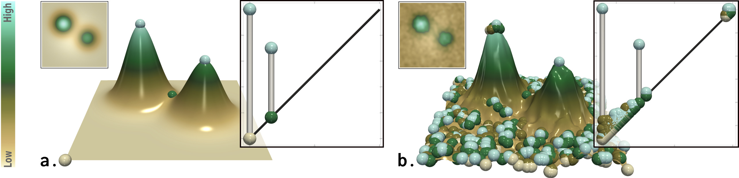
Figure 1: Critical points (spheres, light brown: minima, light green: maxima, other: saddles) and persistence diagrams of a clean (a) and noisy (b) 2D scalar field. From left to right : 2D data, 3D terrain visualization, persistence diagram. In both cases, the two main hills are clearly represented by salient persistence pairs in the diagrams. In the noisy diagram (b), small pairs near the diagonal correspond to noisy features in the data.

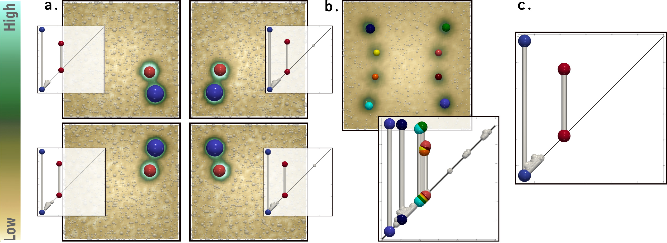
Figure 2: Synthetic ensemble of a pattern with 2 gaussians and additive noise (a). The persistence diagram of the pointwise mean (b) contains 8 highly persistent features although each of the input ensemble members contain only 2 features. The Wasserstein barycenter (c) provides a diagram which is representative of the set, with a feature number, range and salience which better describes the input ensemble (2 large features).

Ensemble visualization: Another category of approaches has been studied to specifically visualize the main trends in ensemble data. In this context, the data variability is directly encoded by a series of global empirical observations (i.e. the members of the ensemble). Existing visualization techniques typically construct geometrical objects, such as level sets or streamlines, for each member of the ensemble. Then, given this ensemble of geometrical objects, the question of estimating an object which is representative of the ensemble naturally arises. For this, several methods have been proposed, such as spaghetti plots [26] in the case of level-set variability in weather data ensemble [76, 82], or box-plots for the variability of contours [95] and curves in general [61]. For the specific purpose of trend variability analysis, Hummel et al. [47] developed a Lagrangian framework for classification in flow ensembles. Related to our work, clustering techniques have been used to analyze the main trends in ensembles of streamlines[34] and isocontours [35]. However, only few techniques have focused on applying this strategy to topological objects. Overlap-based heuristics have been investigated to estimate a representative contour tree from an ensemble [96, 52]. Favelier et al. [32] introduced an approach to analyze critical point variability in ensembles. It relies on the spectral clustering of the ensemble members according to their persistence map, a scalar field defined on the input geometry which characterizes the spatial layout of persistent critical points. However, the clustering stage of this approach takes as an input a distance matrix between the persistence maps of all the members of the ensemble, which requires to mantain them all in memory, which is not conceivable for large-scale ensembles counting a high number of members. Moreover, the clustering itself is performed on the spectral embedding of the persistence maps, where distances are loose approximations of the intrinsic metric between these objects. In contrast, the clustering application described in this paper directly operates on the persistence diagrams of the ensemble members, whose memory footprint is orders of magnitude smaller than the actual ensemble data. This makes our approach more practical, in particular in the perspective of an in-situ computation [8] of the persistence diagrams. Also, it is built on top of our progressive algorithm for Wasserstein barycenters, which focuses on the Wasserstein metric between diagrams. Optionally, our work can also integrate the spatial layout of critical points by considering a geometrically lifted version of this metric [86].

Persistence diagram processing: To define the barycenter of a set of persistence diagrams, a metric (i) first needs to be introduced to measure distances between them. Then, barycenters (ii) can be formally defined as minimizers of the sum of distances to the set of diagrams.

(i) The estimation of distances between topological abstractions has been a long-studied problem, in particular for similarity estimation tasks. Several heuristical approaches have been documented for the fast estimation of structural similarity [46, 91, 81, 90]. More formal approaches have studied various metrics between topological abstractions, such as Reeb graphs [9, 10] or merge trees [11]. For persistence diagrams, the Bottleneck [22] and Wasserstein distances [62, 49, 27], have been widely studied, for instance in machine learning [23] and adapted for kernel based methods [78, 20, 79]. The numerical computation of the Wasserstein distance between two persistence diagrams requires to solve an optimal assignment problem between them. The typical methods for this are the exact Munkres algorithm [64], or an auction-based approach [12] that provides an approximate result with improved time performance. Kerber et al. [51] specialized the auction algorithm to the case of persistence diagrams and showed how to significantly improve performances by leveraging adequate data structures for proximity queries. Soler et al. [86] introduced a fast extension of the Munkres approach, also taking advantage of the structure of persistence diagrams, in order to solve the assignment problem in an exact and efficient way, using a reduced, sparse and unbalanced cost matrix.

(ii) Recent advances in optimal transport [23] enabled the practical resolution of transportation problems between continuous quantities [24, 87]. These methods have been successfully applied to persistence diagrams [53]. However, this application requires to represent the input diagrams as heat maps of fixed resolution [2]. Such a rasterization can be interpreted as a pre-normalization of the diagrams, which can be problematic for applications where the considered diagrams have different persistence scales, as typically found with time-varying phenomena for instance. Moreover, this approach does not explicitly produce a persistence diagram as an output, but a heat map of the population of persistence pairs in the barycenter. This challenges its usage for visualization applications, as the features of interest in the barycenter cannot be directly inferred from the barycenter heat map. In contrast, our approach produces explicitly a persistence diagram as an output, from which the geometry of the features (their number, data ranges and salience) can be directly visually inspected. Moreover, such an explicit representation also enables the efficient geometrical lifting of the Wasserstein metric [86], which is relevant for scientific visualization applications but which would require to regularly sample a five dimensional space with heat map based approaches. Turner et al. [94] introduced an algorithm for the computation of a Fréchet mean of a set of persistence diagrams with regard to the Wasserstein metric. This approach provides explicit barycenters, which makes it appealing for the applications. However, its very high computational cost makes it impractical for real-life data sets. In particular, it is based on an iterative procedure, for which each iteration relies itself on $N$ optimal assignment problems [64] between persistence diagrams (for the Wasserstein distances), where $N$ is the number of members in the ensemble. A naive approach to address this computational bottleneck would be to combine this method with the efficient algorithms for Wasserstein distances mentioned previously [51, 86]. However, as shown in Sec. 5, such a naivean approach is still computationally expensive and it can require up to hours of computation on certain data sets. In contrast, our algorithm converges in multi-threaded mode in a couple of minutes at most, and its progressive nature additionally allows for its interruption within interactive times, while still providing qualitatively meaningful results.

0.2 Contributions

This paper makes the following new contributions:

1. A progressive algorithm for Wasserstein barycenters of persistence diagrams: We present We extend existing work on Fréchet means of persistence diagrams [94] and revisit the fast approximation of Wasserstein distances [12, 51] in order to provide We revisit efficient algorithms for Wasserstein distance approximation [12, 51] in order to extend previous work on barycenter estimation [94]. In particular, we introduce a new algorithmapproach based on a progressive approximation strategy, which iteratively refines both computation accuracy and output details. The persistence pairs of the input diagrams are progressively considered in decreasing order of persistence. This focuses the computation towards the most salient features of the ensemble, while considering noisy persistent pairs last. The returned barycenters are explicit and provide insightful visual hints about the features present in the ensemble. We show that ourOur progressive strategy drastically accelerates convergence in practice, resulting in an order of magnitude speedup over the fastest combinations of existing techniques. The algorithm is trivially parallelizable, which provides additional speedups in practice on standard workstations. Additionally, the progressivity allows to broaden the above algorithm to support computation time constraints, and produce barycenters accounting for the main features of the data within interactive times. We present an interruptible extension of our algorithm to support computation time constraints. This enables to produce barycenters accounting for the main features of the data within interactive times.

2. An interruptible algorithm for the clustering of persistence diagrams: We extend the above methods to revisit the $k$-means algorithm and introduce an interruptible clustering of persistence diagrams, which is used for the visual analysis of the global feature trends in ensembles.

3. Implementation: We provide a lightweight C++ implementation of our algorithms that can be used for reproduction purposes.

1 Preliminaries

This section presents the theoretical background of our approach. It contains definitions adapted from the Topology ToolKit [92]. It also provides, for self completeness, concise descriptions of the key algorithms [94, 51] that our work extends. We refer the reader to Edelsbrunner and Harer [27] for an introduction to computational topology.

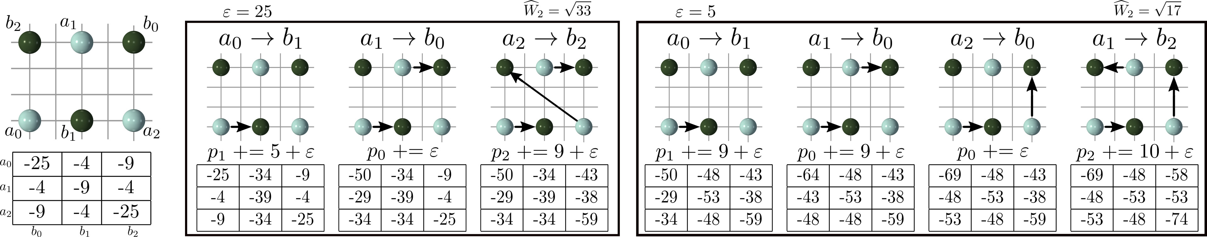
Figure 3: Illustration of the Auction algorithm [12] on a 2D example for the optimal assignment of 2 point sets (light and dark green). Boxes and columns represent auction rounds and auction iterations respectively. Each matrix reports the value $v_{a\rightarrow b}$ currently estimated by the bidder $a$ for the purchase of the object $b$. Assignments are shown with black arrows. After the first round (left box), a sub-optimal assignment is achieved, which becomes optimum at the second round (right box). Note that bidders can steal objects from each other within one auction round (iteration $3$, second round).

1.1 Persistence diagrams

The input data is an ensemble of $N$ piecewise linear (PL) scalar fields $f:\mathscr{M}\rightarrow\mathbb{R}$ defined on a PL $d$-manifold $\mathscr{M}$, with $d\leq 3$ in our applications. We note $f^{-1}_{-\infty}(w)=\{p\in\mathscr{M}~{}|~{}f(p)<w\}$ the sub-level set of $f$, namely the pre-image of $(-\infty,w)$ by $f$. When continuously increasing $w$, the topology of $f^{-1}_{-\infty}(w)$ can only change at specific locations, called the critical points of $f$. In practice, $f$ is enforced to be injective on the vertices of $\mathscr{M}$ [30], which are in finite number. This guarantees that the critical points of $f$ are isolated and also in finite number. Moreover, they are also enforced to be non-degenerate, which can be easily achieved with local re-meshing [28]. Critical points are classified according to their index $\mathscr{I}$ : 0 for minima, 1 for 1-saddles, $d-1$ for $(d-1)$-saddles, and $d$ for maxima. Each topological feature of $f^{-1}_{-\infty}(w)$ (i.e. connected component, independent cycle, void) can be associated with a unique pair of critical points $(c,c^{\prime})$, corresponding to its birth and death. Specifically, the Elder rule [27] states that critical points can be arranged according to this observation in a set of pairs, such that each critical point appears in only one pair $(c,c^{\prime})$ such that $f(c)<f(c^{\prime})$ and $\mathscr{I}{c}=\mathscr{I}{c^{\prime}}-1$. Intuitively, this rule implies that if two topological features of $f^{-1}_{-\infty}(w)$ (e.g. two connected components) meet at a critical point $c^{\prime}$, the youngest feature (i.e. created last) dies, favoring the oldest one (i.e. created first). Critical point pairs can be visually represented by the persistence diagram, noted $\mathscr{D}(f)$, which embeds each pair to a single point in the 2D plane at coordinates $\big{(}f(c),f(c^{\prime})\big{)}$, which respectively correspond to the birth and death of the associated topological feature. The persistence of a pair, noted $\mathscr{P}(c,c^{\prime})$, is then given by its height $f(c^{\prime})-f(c)$. It describes the lifetime in the range of the corresponding topological feature. The construction of the persistence diagram is often restricted to a specific type of pairs, such as $(0,1)$ pairs or $\big{(}(d-1),d\big{)}$ pairs, respectively capturing features represented by minima or maxima. In the following, we will consider that each persistence diagram is only composed of pairs of a fixed critical type $\big{(}(\mathscr{I}-1),\mathscr{I})$, which will be systematically detailed in the experiments. Note that in practice, each critical point in the diagram additionally stores its 3D coordinates in $\mathscr{M}$ to allow geometrical lifting (Sec. 1.2).

In practice, critical point pairs often directly correspond to features of interest in the applications and their persistence has been shown to be a reliable importance measure to discriminate noise from important features. In the diagram, the pairs located in the vicinity of the diagonal represent low amplitude noise while salient features will be associated with persistent pairs, standing out far away from the diagonal (Fig. 1) . For instance, in Fig. 1, the two hills are captured by two large pairs, while noise is encoded with smaller pairs near the diagonal. Thus, the persistence diagram has been shown in practice to be a useful, concise visual representation of the population of features of interest in the data, for which the number, range values and salience can be directly and visually read. In addition to its stability properties [22], these observations motivate its usage for data summerization, where it significantly help users distinguish salient features from noise. In the following, we review distances between persistence diagrams [22, 27] (Sec. 1.2), efficient algorithms for their approximation [12, 51] (Sec. 1.3), as well as the reference approach for barycenter estimation [94] (Sec. 1.4).

1.2 Distances between Persistence diagrams

To compute the barycenter of a set of persistence diagrams, a necessary ingredient is the notion of distance between them. Given two diagrams $\mathscr{D}(f)$ and $\mathscr{D}(g)$, a pointwise distance, noted $d_{q}$, inspired from the $L^{p}$ norm, can be introduced in the 2D birth/death space between two points $a=(x_{a},y_{a})\in\mathscr{D}(f)$ and $b=(x_{b},y_{b})\in\mathscr{D}(g)$, with $q>0$, as follows :

$$d_{q}(a,b)=\left(|x_{b}-x_{a}|^{q}+|y_{b}-y_{a}|^{q}\right)^{1/q}=\|a-b\|_{q}$$ (1)

By convention, $d_{q}(a,b)$ is set to zero if both $a$ and $b$ exactly lie on the diagonal ($x_{a}=y_{a}$ and $x_{b}=y_{b}$). The $q$-Wasserstein distance [49, 62], noted $W_{q}$, between $\mathscr{D}(f)$ and $\mathscr{D}(g)$ can then be introduced as:

$$W_{q}\big{(}\mathscr{D}(f),\mathscr{D}(g)\big{)}=\min_{\phi\in\Phi}\left(\sum_{a\in\mathscr{D}(f)}d_{q}\big{(}a,\phi(a)\big{)}^{q}\right)^{1/q}$$ (2)

where $\Phi$ is the set of all possible assignments $\phi$ mapping each point $a\in\mathscr{D}(f)$ to a point $b\in\mathscr{D}(g)$, or to the closest diagonal pointits projection onto the diagonal, $\Delta(a)=(\frac{x_{a}+y_{a}}{2},\frac{x_{a}+y_{a}}{2})$, which denotes the removal of the corresponding feature from the assignment, with a cost $d_{q}\big{(}a,\Delta(a)\big{)}^{q}$ (see additional materials for an illustration). The Wasserstein distance can be computed by solving an optimal assignment problem, for which existing algorithms [64, 63] however often require a balanced setting. To address this, the input diagrams $\mathscr{D}(f)$ and $\mathscr{D}(g)$ are typically augmented into $\mathscr{D}^{\prime}(f)$ and $\mathscr{D}^{\prime}(g)$, which are obtained by injecting the diagonal projections of all the points of one diagram into the other:

$$\mathscr{D}^{\prime}(f)=\mathscr{D}(f)\cup\{\Delta(b)~{}|~{}b\in\mathscr{D}(g)\}$$ (3)

$$\mathscr{D}^{\prime}(g)=\mathscr{D}(g)\cup\{\Delta(a)~{}|~{}a\in\mathscr{D}(f)\}$$ (4)

In this way, the Wasserstein distance is guaranteed to be preserved by construction, $W_{q}\big{(}\mathscr{D}(f),\mathscr{D}(g)\big{)}=W_{q}\big{(}\mathscr{D}^{\prime}(f),\mathscr{D}^{\prime}(g)\big{)}$, while making the assignment problem balanced ($|\mathscr{D}^{\prime}(f)|=|\mathscr{D}^{\prime}(g)|$) and thus solvable with traditional assignment algorithms. Note that wWhen $q\rightarrow\infty$, $W_{q}$ becomes a worst case assignment distance called the Bottleneck distance [22]., which is often interpreted in practice as less informative, however, than the Wasserstein distance. In the following, we will focus on $q=2$.

In the applications, it can often be useful to geometrically lift the Wasserstein metric, by also taking into account the geometrical layout of critical points [86]. Let $(c,c^{\prime})$ be the critical point pair corresponding the point $a\in\mathscr{D}(f)$. Let $p_{a}^{\lambda}\in\mathbb{R}^{d}$ be their linear combination with coefficient $\lambda\in[0,1]$ in $\mathscr{M}$: $p_{a}^{\lambda}=\lambda c^{\prime}+(1-\lambda)c$. Our experiments (Sec. 5) only deal with extrema, and we set $\lambda$ to $0$ for minima and $1$ for maxima (to only consider the extremum’s location). Then, the geometrically lifted pointwise distance $\widehat{d_{2}}(a,b)$ can be given as:

$$\widehat{d_{2}}(a,b)=\sqrt{(1-\alpha)d_{2}(a,b)^{2}+\alpha||p_{a}^{\lambda}-p_{b}^{\lambda}||_{2}^{2}}$$ (5)

The parameter $\alpha\in[0,1]$ quantifies the importance that is given to the geometry of critical points and it must be tuned on a per application basis. When $\alpha=1$, the combination of $W_{2}$ with $\widehat{d_{2}}$ becomes the classical Earth Mover’s distance [DBLP:conf/iccv/LevinaB01] between critical points in $\mathscr{M}$ and $\alpha$ thus enables users to simply linearly blend these two metrics.

1.3 Efficient distance computation by Auction

This section briefly describes a fast approximation of Wasserstein distances by the auction algorithm [12, 51], which is central to our method.

The assignment problem involved in Eq. 2 can be modeled in the form of a weighted bipartite graph, where the points $a\in\mathscr{D}^{\prime}(f)$ are represented as nodes, connected by edges to nodes representing the points of $b\in\mathscr{D}^{\prime}(g)$, with an edge weight given by $d_{2}(a,b)^{2}$ (Eq. 1). To efficiently estimate the optimal assignment, Bertsekas introduced the auction algorithm [12] (Fig. 3), which replicates the behavior of a real-life auction: the points of $\mathscr{D}^{\prime}(f)$ are acting as bidders that iteratively make offers for the purchase of the points of $\mathscr{D}^{\prime}(g)$, known as the objects. Each bidder $a\in\mathscr{D}^{\prime}(f)$ makes a benefit $\beta_{a\rightarrow b}=-d_{2}(a,b)^{2}$ for the purchase of an object $b\in\mathscr{D}^{\prime}(g)$, which is itself labeled with a price $p_{b}\geq 0$, initially set to $0$. During the iterations of the auction, each bidder $a$ tries to purchase the object $b$ of highest value $v_{a\rightarrow b}=\beta_{a\rightarrow b}-p_{b}$. The bidder $a$ is then said to be assigned to the object $b$. If $b$ was previously assigned, its previous owner becomes unassigned. At this stage, the price of $b$ is increased by $\delta_{a}+\epsilon$, where $\delta_{a}$ is the absolute difference between the two highest values $v_{a\rightarrow b}$ that the bidder $a$ found among the objects $b$, and where $\epsilon>0$ is a constant. This bidding procedure is repeated iteratively among the bidders, until all bidders are assigned (which is guaranteed to occur by construction, thanks to the $\epsilon$ constant). At this point, we sayit is said that an auction round has completed: a bijective, possibly sub-optimal, assignement $\phi$ exists between $\mathscr{D}^{\prime}(f)$ and $\mathscr{D}^{\prime}(g)$. The overall algorithm will repeat auction rounds, which progressively increases prices under the effect of competing bidders.

The constant $\epsilon$ plays a central role in the auction algorithm. Let $\widehat{W_{2}}\big{(}\mathscr{D}^{\prime}(f),\mathscr{D}^{\prime}(g)\big{)}=\sqrt{\sum_{a\in\mathscr{D}^{\prime}(f)}d_{2}\big{(}a,\phi(a)\big{)}^{2}}$ be the approximation of the Wasserstein distance $W_{2}\big{(}\mathscr{D}(f),\mathscr{D}(g)\big{)}$, obtained with the assignment $\phi$ returned by the algorithm. Large values of $\epsilon$ will drastically accelerate convergence (as they imply fewer iterations for the construction of a bijective assignment $\phi$ within one auction round, Fig. 3), while low values will improve the accuracy of $\widehat{W_{2}}$. This observation is a key insight at the basis of our approach. Bertsekas suggests a strategy called $\epsilon$-scaling, which decreases $\epsilon$ after each auction round. In particular, if:

$$\widehat{W_{2}}\big{(}\mathscr{D}^{\prime}(f),\mathscr{D}^{\prime}(g)\big{)}^{2}\leq(1+\gamma)^{2}\Big{(}\widehat{W_{2}}\big{(}\mathscr{D}^{\prime}(f),\mathscr{D}^{\prime}(g)\big{)}^{2}-\epsilon|\mathscr{D}^{\prime}(f)|\Big{)}$$ (6)

then it can be shown that [13, 51]:

$$W_{2}\big{(}\mathscr{D}(f),\mathscr{D}(g)\big{)}\leq\widehat{W_{2}}\big{(}\mathscr{D}^{\prime}(f),\mathscr{D}^{\prime}(g)\big{)}\leq(1+\gamma)W_{2}\big{(}\mathscr{D}(f),\mathscr{D}(g)\big{)}$$ (7)

This result is particularly important, as it enables to estimate the optimal assignment, and thus the Wasserstein distance, with an on-demand accuracy (controlled by the parameter $\gamma$) by using Eq. 6 as a stopping condition for the overall auction algorithm. For persistence diagrams, Kerber et al. showed how the computation could be accelerated by using space partitioning data structures such as kd-trees [51]. In practice, we set $\epsilon$ to be initially $\epsilon$ is initially set to be equal to $1/4$ of the largest edge weight $d_{2}(a,b)^{2}$, we divide itand is divided by $5$ after each auction round, as recommended by Bertsekas [12], and we. We use $\gamma=0.01$ $\gamma$ is set to $0.01$ as suggested by Kerber et al. [51].

Algorithm 1 Reference algorithm for Wasserstein Barycenters [94].

Input : Set of diagrams $\mathscr{F}=\{\mathscr{D}(f_{1}),\mathscr{D}(f_{2}),\dots,\mathscr{D}(f_{N})\}$

Output : Wasserstein barycenter $\mathscr{D}^{*}$

1:  $\mathscr{D}^{*}\leftarrow\mathscr{D}(f_{i})\quad\quad\quad\quad\quad\quad\quad\quad\quad\quad\quad\quad\quad\quad\quad$ // with $i$ randomly chosen in $[1,N]$

2:  while $\{\phi_{1},\phi_{2},\dots,\phi_{N}\}$ change do

3:     // Relaxation start

4:     for $i\in[1,N]$ do

5:        $\phi_{i}\leftarrow Assignment\big{(}\mathscr{D}(f_{i}),\mathscr{D}^{*}\big{)}\quad~{}\quad\quad\quad\quad\quad\quad\quad\quad\quad\quad$ // optimizing Eq. 2

6:     end for

7:     $\mathscr{D}^{*}\leftarrow Update(\phi_{1},\dots,\phi_{n})\quad\quad\quad\quad\quad\quad$ // arithmetic means in birth/death space

8:     // Relaxation end

9:  end while

10:  return  $\mathscr{D}^{*}$

1.4 Wasserstein barycenters of Persistence diagrams

Let $\mathbb{D}$ be the space of persistence diagrams. The discrete Wasserstein barycenter of a set $\mathscr{F}=\{\mathscr{D}(f_{1}),\mathscr{D}(f_{2}),\dots,\mathscr{D}(f_{N})\}$ of persistence diagrams can be introduced as the Fréchet mean of the set, under the metric $W_{2}$. It is the diagram $\mathscr{D}^{*}$ that minimizes its distance to all the diagrams of the set (i.e. minimizer of the so-called Fréchet energy):

$$\mathscr{D}^{*}=\operatorname*{arg\,min}_{\mathscr{D}\in\mathbb{D}}\sum_{\mathscr{D}(f_{i})\in\mathscr{F}}W_{2}\big{(}\mathscr{D},\mathscr{D}(f_{i})\big{)}^{2}$$ (8)

The computation of Wasserstein barycenters involves a computationally demanding optimization problem, for which the existence of at least one locally optimum solution has been shown by Turner et al. [94], who also introduced the first algorithm for its computation. This algorithm (Alg. 1) consists in iterating a procedure that we call Relaxation (line 3 to 8), which resembles a Lloyd relaxation [56], and which is composed itself of two sub-routines: (i) Assignment (line 5) and (ii) Update (line 7). Given an initial barycenter candidate $\mathscr{D}$ randomly chosen among the set $\mathscr{F}$, the first step ((i) Assignment) consists in computing an optimal assignment $\phi_{i}:\mathscr{D}\rightarrow\mathscr{D}(f_{i})$ between $\mathscr{D}$ and each diagram $\mathscr{D}(f_{i})$ of the set $\mathscr{F}$, with regard to Eq. 2. The second step ((ii) Update) consists in updating the candidate $\mathscr{D}$ to a position in $\mathbb{D}$ which minimizes the sum of its squared distances to the diagrams of $\mathscr{F}$ under the current set of assignments $\{\phi_{1},\phi_{2},\dots,\phi_{N}\}$. In practice, this last step is achieved by simply replacing each point $a\in\mathscr{D}$ by the arithmetic mean (in the birth/death space) of all its assignments $\phi_{i}(a)$. The overall algorithm continues to iterate the Relaxation procedure until the set of optimal assignments $\phi_{i}$ remains identical for two consecutive iterations.

1.5 Overview of our approach

The reference algorithm for Wasserstein barycenters (Alg. 1) reveals impractical for real-life data sets. Its main computational bottleneck is the Assignment step, which involves the computation of $N$ Wasserstein distances (Eq. 2). However, as detailed in the result section (Sec. 5), even when combined with efficient algorithms for the Wasserstein distance exact computation [86] or even approximation [51] (Sec. 1.3), this overall method can still lead to hours of computation in practice.

Thus, a drastically different approach is needed to improve computation efficiency, especially for applications such as ensemble clustering, which require multiple barycenter estimations per iteration.

In this work, we introduce a novel progressive framework for Wasserstein barycenters, which is based on two key observations. First, from one Relaxation iteration to the next (lines 3 to 8, Alg. 1), the estimated barycenter is likely to vary only slightly. This motivates the design of a faster algorithm for the Assignment step, which would be capable of starting its optimization from a relevant initial assignment, typically given in our setting by the previous Relaxation iteration. Second, in the initial Relaxation iterations, the estimated barycenter can be arbitrarily far from the final, optimized barycenter. Thus, for these iterations, it can be beneficial to relax the level of accuracy of the Assignment step, which is the main bottleneck, and to progressively increase it when it is the most needed, as the barycenter converges to a solution.

2 Progressive Barycenters

This section presents our novel progressive framework for the approximation of Wasserstein barycenters of a set of Persistence diagrams $\mathscr{F}=\{\mathscr{D}(f_{1}),\mathscr{D}(f_{2}),\dots,\mathscr{D}(f_{N})\}$. As mentioned above, the key insights of our approach are twofolds. First, the assignments involved in the Wasserstein distance estimations can be re-used as initial conditions along the iterations of the barycenter Relaxation (Sec. 3.2). Second, progressivity can be injected in the process to accelerate convergence, by adequately controlling the level of accuracy in the evaluation of the Wasserstein distances along the Relaxation iterations of the barycenter. This progressivity can be injected at two levels: by controlling the accuracy of the distance estimation itself (Sec. 3.3) and the resolution of the input diagrams (Sec. 3.4). The rest of the section presents a parallelization of our framework (Sec. 3.5) and describes an interruptible algorithm, capable of respecting running time constraints (Sec. 3.6).

3 Progressive Barycenters

This section presents our novel progressive framework for the approximation of Wasserstein barycenters of a set of Persistence diagrams$\mathscr{F}=\{\mathscr{D}(f_{1}),\mathscr{D}(f_{2}),\dots,\mathscr{D}(f_{N})\}$..

3.1 Overview

The key insights of our approach are twofolds. First, in the reference algorithm (Alg. 1), from one Relaxation iteration to the next (lines 3 to 8), the estimated barycenter is likely to vary only slightly. Previous assignments can thus Thus, the assignments involved in the Wasserstein distance estimations can be re-used as initial conditions along the iterations of the barycenter Relaxation (Sec. 3.2). Second, in the initial Relaxation iterations, the estimated barycenter can be arbitrarily far from the final, optimized barycenter. Thus, for these early iterations, it can be beneficial to relax the level of accuracy of the Assignment step, which is the main bottleneck, and to progressively increase it as the barycenter converges to a solution. Progressivity can be injected at two levels: by controlling the accuracy of the distance estimation itself (Sec. 3.3) and the resolution of the input diagrams (Sec. 3.4). Our framework is easily parallelizable (Sec. 3.5) and the progressivity allows to design an interruptible algorithm, capable of respecting running time constraints (Sec. 3.6).

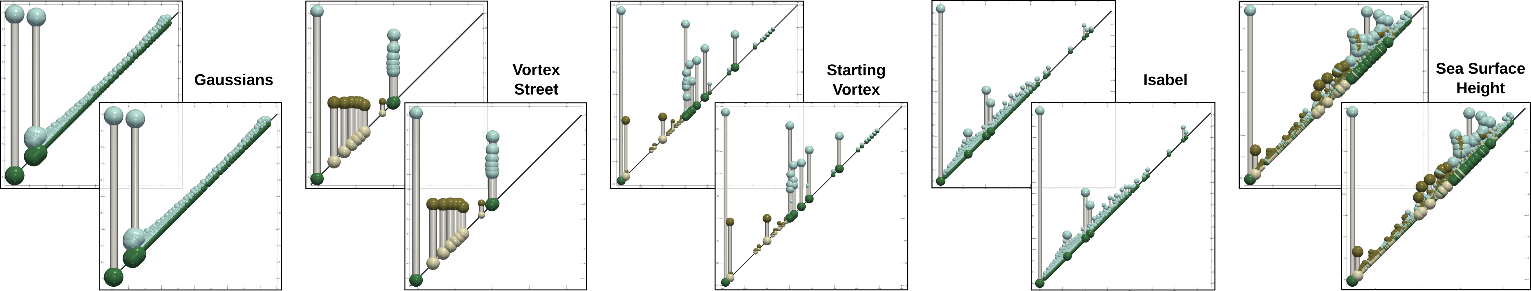
Figure 4: Visual comparison between the converged Wasserstein barycenters obtained with the Auction barycenter algorithm [94]+[51](top) and our approach (bottom) for one cluster (Sec. 5.3) of each ensemble data set. Differences are barely noticeable, and only for small persistence pairs.

3.2 Auctions with Price Memorization

The Assignment step of the Wasserstein barycenter computation (line 5, Alg. 1) can be resolved in principle with any of the existing techniques for Wasserstein distance estimation [64, 63, 51, 86]. Among them, the Auction based approach [12, 51] (Sec. 1.3) is particularly relevant as it can compute very efficiently approximations with on-demand accuracy.

In the following, we consider that each distance computation involves augmented diagrams (Sec. 1.2). Each input diagram $\mathscr{D}(f_{i})\in\mathscr{F}$ is then considered as a set of bidders (Sec. 1.3) while the output barycenter $\mathscr{D}^{*}$ contains the objects to purchase. Each input diagram $\mathscr{D}(f_{i})$ maintains its own list of prices $p_{b}^{i}$ for the purchase of the objects $b\in\mathscr{D}^{*}$ by the bidders $a\in\mathscr{D}(f_{i})$. The search by a bidder for the two most valuable objects to purchase is accelerated with space partitioning data structures, by using a kd-tree and a lazy heap respectively for the off- and on-diagonal points [51] (these structures are re-computed for each Relaxation). Thus, the output barycenter $\mathscr{D}^{*}$ maintains only one kd-tree and one lazy heap for this purpose. Since Wasserstein distances are only approximated in this strategy, we suggest to relax the overall stopping condition (Alg. 1) and stop the iterations after two successive increases in Fréchet energy (Eq. 8), as commonly done in gradient descent optimizations. In the rest of the paper, we call the above strategy the Auction barycenter algorithm [94]+[51], as it naivelyjust combines the algorithms by Turner et al. [94] and Kerber et al. [51].

However, this naive usage of the auction algorithm results in a complete reboot of the entire sequence of auction rounds upon each Relaxation, while in practice, for the barycenter problem, the output assignments $\phi_{i}$ may be very similar from one Relaxation iteration to the next and thus could be re-used as initial solutions. For this, we introduce a mechanism that we call Price Memorization, which simply consists in initializing the prices $p_{b}^{i}$ for each bidder $a\in\mathscr{D}(f_{i})$ to the prices obtained at the previous Relaxation iteration (instead of $0$). This has the positive effect of encouraging bidders to bid in priority on objects which were previously assigned to them, hence effectively re-using the previous assignments as an initial solution. This memorization makes most of the early auction rounds become unnecessary in practice, which enables to drastically reduce their number, as detailed in the following.

3.3 Accuracy-driven progressivity

The reference algorithm for Wasserstein barycenter computation (Alg. 1) can also be interpreted as a variant of gradient descent [94]. For such methods, it is often observed that approximations of the gradient, instead of exact computations, can be sufficient in practice to reach convergence. This observation is at the basis of our progressive strategy. Indeed, in the early Relaxation iterations, the barycenter can be arbitrarily far from the converged result and achieving a high accuracy in the Assignment step (line 5) for these iterations is often a waste of computation time. Therefore we introduce a mechanism that progressively increases the accuracy of the Assignment step along the Relaxation iterations, to provide the maximumin order to obtain more accuracy near convergence.

To achieve this, inspired by the internals of the auction algorithm, we apply a global $\epsilon$-scaling (Sec. 1.3), where we progressively decrease the value of $\epsilon$, but only at the end of each Relaxation. Combined with Price Memorization (Sec. 3.2), this strategy enables us to perform only one auction round per Assignment step. As large $\epsilon$ values accelerate auction convergence at the price of accuracy, this strategy effectively speeds up the early Relaxation iterations and leads to more and more accurate auctions, and thus assignments, along the Relaxation iterations.

In practice, we divide $\epsilon$ by $5$ after each Relaxation, as suggested by Bertsekas [12] in the case of the regular auction algorithm (Sec. 1.3). Moreover, to guarantee precise final barycenters (obtained for small $\epsilon$ values), we modify the overall stopping condition to prevent the algorithm from stopping if $\epsilon$ is larger than $10^{-5}$ of its initial value.

Table 1: Comparison of running times (in seconds, 1 thread) for the estimation of Wasserstein barycenters of Persistence diagrams. $N$ and $\#_{\mathscr{D}(f_{i})}$ respectively stand for the number of members in the ensemble and the average size of the input persistence diagrams.

Data set	$N$	$\#_{\mathscr{D}(f_{i})}$	10cm Sinkhorn
[53]	10cm Munkres
[94]+[86]	10cmAuction
[94]+[51]	Ours	Speedup
Gaussians (Fig. 7)	100	2,078	7,499.33	$>24$H	8,975.60	785.53	11.4
Vortex Street (Fig. 8)	45	14	54.21	0.14	0.47	0.23	0.6
Starting Vortex (Fig. 9)	12	36	40.98	0.06	0.67	0.28	0.2
Isabel (3D) (Progressive Wasserstein Barycenters of Persistence Diagrams)	12	1,337	1,070.57	$>24$H	377.42	82.95	4.5
Sea Surface Height (Fig. 10)	48	1,379	4,565.37	$>24$H	949.08	75.90	12.5

3.4 Persistence-driven progressivity

In practice, the persistence diagrams of real-life data sets often contain a very large number of critical point pairs of low persistence. These numerous small pairs correspond to noise and are often meaningless for the applications. However, although they individually have only little impact on Wasserstein distances (Eq. 2), their overall contributions may be non-negligible. To account for this, we introduce in this section a persistence-driven progressive mechanism, which progressively inserts in the input diagrams critical point pairs of decreasing persistence. This focuses the early Relaxation iterations on the most salient features of the data, while considering the noisy ones last. In practice, this encourages the optimization to explore more relevant local minima of the Fréchet energy (Eq. 8) that favor persistent features.

Given an input diagram $\mathscr{D}(f_{i})$, let $\mathscr{D}_{\rho}(f_{i})$ be the subset of its points with persistence higher than $\rho$: $\mathscr{D}_{\rho}(f_{i})=\{a\in\mathscr{D}(f_{i})~{}|~{}y_{a}-x_{a}>\rho\}$. To account for persistence-driven progressivity, we run our barycenter algorithm (with Price Memorization, Sec. 3.2, and accuracy-driven progressivity, Sec. 3.3) by initially considering as an input the diagrams $\mathscr{D}_{\rho}(f_{i})$. After each Relaxation iteration (Alg. 2, line 10), we decrease $\rho$ such that $|\mathscr{D}_{\rho}(f_{i})|$ does not increase by more than 10% (to progress at uniform speed) and such that $\rho$ does not get smaller than $\sqrt{\tau\epsilon}$ (we set $\tau=4$ to replicate locally Bertsekas’s suggestion for $\epsilon$ setting, Sec. 1.3). Initially, $\rho$ is set to half of the maximum persistence found in the input diagrams. Along the Relaxation iterations, the input diagrams $\mathscr{D}_{\rho}(f_{i})$ are progressively populated, which yields the introduction of new points in the barycenter $\mathscr{D}^{*}$, which we initialize at locations selected uniformly among the newly introduced points of the $N$ inputs. This strategy enables to distribute among the inputs the initialization of the new barycenter points. The corresponding prices are initialized with the minimum price $p_{b}^{i}$ found for the objects $b\in\mathscr{D}^{*}$ at the previous iteration.

Algorithm 2 Our overall algorithm for Progressive Wasserstein Barycenters.

Input : Set of diagrams $\mathscr{F}=\{\mathscr{D}(f_{1}),\mathscr{D}(f_{2}),\dots,\mathscr{D}(f_{N})\}$, time constraint $t_{max}$

Output : Wasserstein barycenter $\mathscr{D}^{*}_{\rho}$

1:  $\mathscr{D}^{*}_{\rho}\leftarrow\mathscr{D}_{\rho}(f_{i})\quad\quad\quad\quad\quad\quad\quad\quad\quad\quad\quad\quad\quad\quad\quad$ // with $i$ randomly chosen in $[1,N]$

2:  while the Fréchet energy decreases do

3:     // Relaxation start

4:     for $i\in[1,N]$ do

5:        // In parallel                                                                  // Sec. 3.5

6:        $\phi_{i}\leftarrow Assignment\big{(}\mathscr{D}_{\rho}(f_{i}),\mathscr{D}^{*}_{\rho}\big{)}\quad\quad~{}\quad\quad\quad\quad\quad\quad\quad\quad\quad\quad\quad~{}~{}~{}$ // Sec. 3.2

7:     end for

8:     $\mathscr{D}^{*}_{\rho}\leftarrow Update(\phi_{1},\dots,\phi_{n})\quad\quad\quad\quad\quad\quad$ // arithmetic means in birth/death space

9:     $EpsilonScaling()\quad\quad\quad\quad\quad\quad\quad\quad\quad\quad\quad\quad\quad\quad\quad\quad\quad\quad\quad\quad~{}~{}~{}$ // Sec. 3.3

10:     if $t<0.1\times t_{max}$ then $PersistenceScaling()\quad\quad~{}~{}~{}\quad\quad\quad\quad\quad\quad\quad\quad$ // Sec. 3.4

11:     else if $t>=t_{max}$ then return $\mathscr{D}^{*}_{\rho}\quad\quad\quad\quad\quad\quad~{}~{}\quad\quad\quad\quad\quad\quad\quad\quad$ // Sec. 3.6

12:     // Relaxation end

13:  end while

14:  return  $\mathscr{D}^{*}_{\rho}$

3.5 Parallelism

Our progressive framework can be trivially parallelized as the most computationally demanding task, the Assignment step (Alg. 2), is independent for each input diagram $\mathscr{D}(f_{i})$. The space partitioning data structures used for proximity queries to $\mathscr{D}^{*}$ are accessed independently by each bidder diagram. Thus, we parallelize our approach by running the Assignment step in $n_{t}$ independent threads.

3.6 Computation time constraints

Our persistence-driven progressivity (Sec. 3.4) focuses the early iterations of the optimization on the most salient features, while considering the noisy ones last. However, as discussed before, low persistence pairs in the input diagrams are often considered as meaningless in the applications. This means that our progressive framework can in principle be interrupted before convergence and still provide a meaningful result.

Let $t_{max}$ be a user defined time constraint. We first progressively introduce points in the input diagrams $\mathscr{D}_{\rho}(f_{i})$ and perform the Relaxation iterations for the first $10\%$ of the time constraint $t_{max}$, as described in Sec. 3.4. At this point, the optimized barycenter $\mathscr{D}^{*}$ contains only a fraction of the points it would have contained if computed until convergence. To guarantee a precise output barycenter, we found that continuing the Relaxation iterations for the remaining $90\%$ of the time, without introducing new persistence pairs, provided the best results. Note that iIn practice, in most of our experiments, we observed that this second optimization part fully converged even before reaching $90\%$ of the computation time constraint. Alg. 2 summarizes our overall approach for Wasserstein barycenters of persistence diagrams, with price memorization, progressivity, parallelism and time constraints. For clarity, we provide in the additional materials a toy example of the unfolding of our algorithm. Several iterations of our algorithm are illustrated on a toy example in additional material.

4 Application to Ensemble Topological Clustering

This section presents an application of our progressive framework for Wasserstein barycenters of persistence diagrams to the clustering of the members of ensemble data sets. Since it focuses on persistence diagrams, this strategy enables to group together ensemble members that have the same topological profile, hence effectively highlighting the main trends found in the ensemble in terms of features of interest.

The $k$-means is a popular algorithm for the clustering of the elements of a set, if distances and barycenters can be estimated on this set. The latter is efficiently computable for persistence diagrams thanks to our novel progressive framework and we detail in the following how to revisit the $k$-means algorithm to make it use our progressive barycenters as estimates of the centroids of the clusters.

Table 2: Running times (in seconds) of our approach (run until convergence) with 1 and 8 threads. $N$ and $\#_{\mathscr{D}(f_{i})}$ stand for the number of members in the ensemble and the average size of the diagrams.

Data set	$N$	$\#_{\mathscr{D}(f_{i})}$	1 thread	8 threads	Speedup
Gaussians (Fig. 7)	100	2,078	785.53	117.91	6.6
Vortex Street (Fig. 8)	45	14	0.23	0.10	2.3
Starting Vortex (Fig. 9)	12	36	0.28	0.19	1.5
Isabel (3D) (Progressive Wasserstein Barycenters of Persistence Diagrams)	12	1,337	82.95	31.75	2.6
Sea Surface Height (Fig. 10)	48	1,379	75.90	19.40	3.9

Table 3: Comparison of Fréchet energy (Eq. 8) at convergence between the Auction barycenter method [94]+[51]  and our approach.

Data set	$N$	$\#_{\mathscr{D}(f_{i})}$	10cmAuction
[94]+[51]	Ours	Ratio
Gaussians (Fig. 7)	100	2,078	39.4	39.0	0.99
Vortex Street (Fig. 8)	12	36	415.1	412.5	0.99
Starting Vortex (Fig. 9)	45	14	112,787.0	112,642.0	1.00
Isabel (3D) (Progressive Wasserstein Barycenters of Persistence Diagrams)	12	1,337	2,395.6	2,337.1	0.98
Sea Surface Height (Fig. 10)	48	1,379	7.2	7.1	0.99

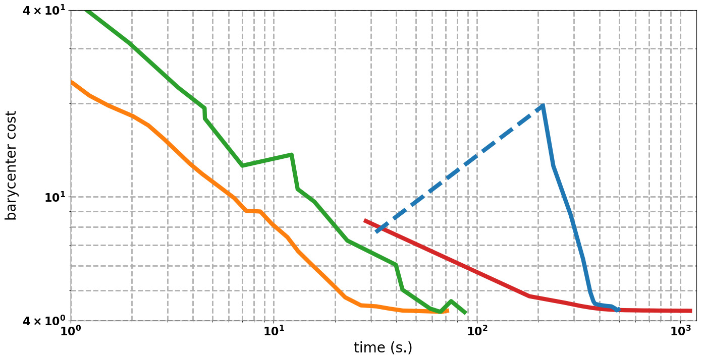
Figure 5: Comparison of the evolution of the Fréchet energy (log scale, Sea Surface Height, maximum diagrams), for the Auction barycenter method [94]+[51](red) and 3 variants of our approach: without (blue) and with (orange) persistence progressivity, and with time constraints (green). Persistence-driven progressivity drastically accelerates convergence.

The $k$-means is an iterative algorithm, which highly resembles barycenter computation algorithms (Sec. 1.4), where each Clustering iteration is composed itself of two sub-routines: (i) Assignment and (ii) Update. Initially, $k$ cluster centroids $\mathscr{D}^{*}_{j}$ ($j\in[1,k]$) are initialized on $k$ diagrams $\mathscr{D}(f_{i})$ of the input set $\mathscr{F}$. For this, in practice, we use the $k$-means++ heuristic described by Celebi et al. [21], which aims at maximizing the distance between centroids. Then, the Assignment step consists in assigning each diagram $\mathscr{D}(f_{i})$ to its closest centroid $\mathscr{D}^{*}_{j}$. This implies the computation, for each diagram $\mathscr{D}(f_{i})$ of its Wasserstein distance $W_{2}$ to all the centroids $\mathscr{D}^{*}_{j},j\in[1,k]$. For this step, we estimate these pairwise distances with the Auction algorithm run until convergence ($\gamma=0.01$, Sec. 1.3). In practice, we use the accelerated $k$-means strategy described by Elkan [31], which exploits the triangle inequality between centroids to skip, given a diagram $\mathscr{D}(f_{i})$, the computation of its distance to centroids $\mathscr{D}^{*}_{j}$ which cannot be the closest. Next, the Update step consists in updating each centroid’s location by placing it at the barycenter (with Alg. 2) of its assigned diagrams $\mathscr{D}(f_{i})$. The algorithm continues these Clustering iterations until convergence, i.e. until the assignments between the diagrams $\mathscr{D}(f_{i})$ and the $k$ centroids $\mathscr{D}^{*}_{j}$ do not evolve anymore, hence yielding the final clustering.

From our experience, the Update step of a Clustering iteration is by far the most computationally expensive. To speed up this stage in practice, we derive a strategy that is similar to our approach for barycenter approximation: we reduce the computation load of each Clustering iteration and progressively increase their accuracy along the optimization. This strategy is motivated by a similar observation: early centroids are quite different from the converged ones, which motivates an accuracy reduction in the early Clustering iterations of the algorithm. Thus, for each Clustering iteration, we use a single round of auction with price memorization (Sec. 3.2), and a single barycenter update (i.e. a single Relaxation iteration, Alg. 2). Overall, only one global $\epsilon$-scaling (Sec. 3.3) is applied at the end of each Clustering iteration. This enhances the $k$-means algorithm with accuracy progressivity. If a diagram $\mathscr{D}(f_{i})$ migrates from a cluster $j$ to a cluster $l$, the prices of the objects of $\mathscr{D}^{*}_{l}$ for the bidders of $\mathscr{D}(f_{i})$ are initialized to $0$ and we run the auction algorithm between $\mathscr{D}(f_{i})$ and $\mathscr{D}^{*}_{l}$ until the pairwise $\epsilon$ value matches the global $\epsilon$ value, in order to obtain prices for $\mathscr{D}(f_{i})$ which are comparable to the other diagrams. Also, we apply persistence-driven progressivity (Sec. 3.4) by adding persistence pairs of decreasing persistence in each diagram $\mathscr{D}(f_{i})$ along the Clustering iterations. Finally, a computation time constraint can also be provided, as described in Sec. 3.6. Results of our clustering scheme are presented in Sec. 5.3.

5 Results

This section presents experimental results obtained on a ècomputer with two Xeon CPUs (3.0 GHz, 2x4 cores), with 64GB of RAM. The input persistence diagrams were computed with the algorithm by Gueunet et al. [37], which is available in the Topology ToolKit (TTK) [92]. the FTM algorithm [37, 92]. We implemented our approach in C++, as TTK modules.

Our experiments were performed on a variety of simulated and acquired 2D and 3D ensembles, ., exactly the same as those used by Favelier et al. [32]. taken from Favelier et al. [32]. The Gaussians ensemble contains 100 2D synthetic noisy members, with 3 patterns of Gaussians (Fig. 7). The considered features of interest in this example are the maxima, hence only the diagrams including the $\big{(}(d-1),d\big{)}$ persistence pairs are considered.. The Vortex Street ensemble (Fig. 8) includes 45 runs of a 2D simulation of flow turbulence behind an obstacle. The considered scalar field is the curl orthogonal component, for 5 fluids of different viscosity(9 runs per fluid, each run with varying Reynolds numbers).. In this application, salient extrema are typically considered as reliable estimations of the center of vortices. Thus, each run is represented by two diagrams, processed independently by our algorithms: one for the $(0,1)$ pairs (involving minima) and one for the $\big{(}(d-1),d\big{)}$ pairs (involving maxima). The Starting Vortex ensemble (Fig. 9) includes 12 runs of a 2D simulation of the formation of a vortex behind a wing, for 2 distinct wing configurations. The considered data is also the curl orthogonal component and diagrams involving minima and maxima are also considered. The Isabel data set (Progressive Wasserstein Barycenters of Persistence Diagrams) is a volume ensemble of 12 members, showing key time steps (formation, drift and landfall) in the simulation of the Isabel hurricane [84]. In this example, the eyewall of the hurricane is typically characterized by high wind velocities, well captured by velocity maxima. Thus we only consider diagrams involving maxima. Finally, the Sea Surface Height ensemble (Fig. 10) is composed of 48 observations taken in January, April, July and October 2012 (https://ecco.jpl.nasa.gov/products/all/). TheHere, the features of interest are the center of eddies, which can be reliably estimated with height extrema. Thus, both the diagrams involving the minima and maxima are considered and independently processed by our algorithms. Unless stated otherwise, all results were obtained by considering the Wasserstein metric $W_{2}$ based on the original pointwise metric (Eq. 1) without geometrical lifting (i.e. $\alpha=0$, Sec. 1.2).

5.1 Time performance

We first evaluate the time performance of our progressive framework when run until convergence (i.e. no computation time constraint). The corresponding timings are reported in Tab. 1. Tab. 1 evaluates the time performance of our progressive framework when run until convergence (i.e. no computation time constraint). This table also provides running times for 3 alternatives. The column, Sinkhorn, provides the timings obtained with a Python CPU implementation kindly provided by Lacombe et al. [53], for which we used the recommended parameter values (entropic term: $10^{-1}/\#_{\mathscr{D}(f_{i})}$ heat map resolution: $100^{2}$). Note that this approach casts the problem as an Eulerian transport optimization under an entropic regularization term. Thus, it optimizes for a convex functional which is considerably different from the Fréchet energy considered in our approach (Eq. 8). Overall, these aspects, in addition to the difference in programming language, challenge direct comparisons and we only report running times for completeness. The columns Munkres, noted [94]+[86], and Auction, noted [94]+[51], report the running times of our own C++ implementation of Turner’s algorithm [94] where distances are respectively estimated with the exact method by Soler et al. [86] (available in TTK [92]) and our own C++ implementation of the auction-based approximation by Kerber et al. [51] (with kd-tree and lazy heap, run until convergence, $\gamma=0.01$).

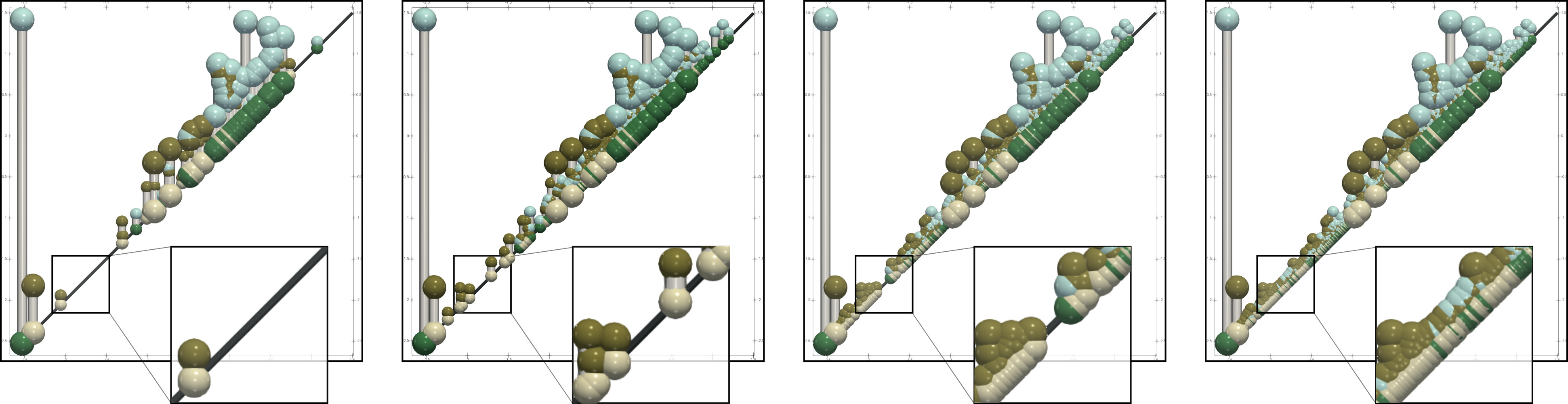
Figure 6: Interrupted Wasserstein barycenters for one cluster of the Sea Surface Height ensemble with different computation time constraints. From left to right : 0.1 s., 1 s., 10 s., and full convergence (21 s.).

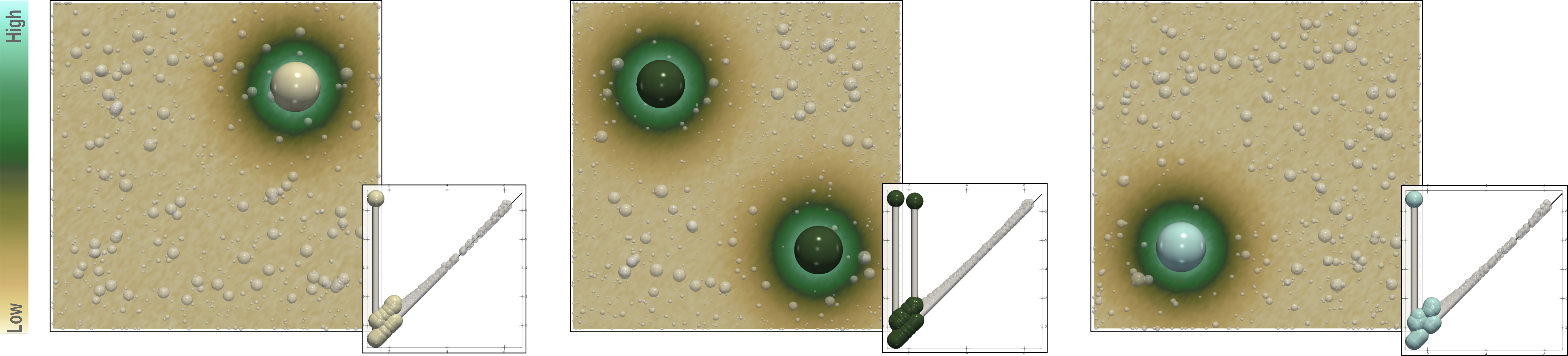
Figure 7: Clustering the Gaussians ensemble. From left to right, pointwise mean and Wasserstein barycenter for each of the identified clusters ($t_{max}:10s.$) with geometrical lifting ($\alpha=0.65$).

As predicted, the cubic time complexity of the Munkres algorithm makes it impractical for barycenter estimation, as the computation completed within 24 hours for only two ensembles(Vortex Street and Starting Vortex), where the diagrams are particularly small.. The Auction approach is more practical but still requires up to hours to converge for the largest data sets. In contrast, our approach converges in sequential in less than 15 minutes at most. The column Speedup reports the gain obtained with our method against the fastest of the two explicit alternatives, Munkres or Auction. For ensembles of realistic size, this speedup is about an order of magnitude. Our approach can be trivially parallelized by running the Assignment step (Alg. 2) in independent threads (Sec. 3.5). We implemented this strategy with OpenMP and the results are reported in Tab. 2. As reported in Tab. 2, our approach can be trivially parallelized with OpenMP by running the Assignment step (Alg. 2) in independent threads (Sec. 3.5). As the size of the input diagrams $\mathscr{D}(f_{i})$ may strongly vary within an ensemble, this trivial parallelization may result in load imbalance among the threads, impairing parallel efficiency. In practice, this strategy still provides reasonable speedups, bringing the computation down to a couple of minutes at most.

5.2 Barycenter quality

Tab. 3 compares the Fréchet energy (Eq. 8) of the converged barycenters for our method and the Auction barycenter alternative [94]+[51] (the Wasserstein distances between the results of the two approaches are provided in additional material for further details). In particular, tThe Fréchet energy has been precisely evaluated with an estimation of Wasserstein distances based on the Auction algorithm run until convergence ($\gamma=0.01$). While the actual values for this energy are not specifically relevant (because of various data ranges), the ratio between the two methods indicates that the local minima approximated by both approaches are of comparable numerical quality, with a variation of $2\%$ in energy at most. Fig. 4 provides a visual comparison of the converged Wasserstein barycenters obtained with the Auction barycenter alternative [94]+[51]  and our method, for one cluster of each of our data sets (Sec. 5.3). This figure shows that differences are barely noticeable and only involve pairs with low persistence, which are often of small interest in the applications.

Fig. 5 detailscompares the convergence rates of the Auction barycenter [94]+[51](red) andto three variants of our framework: without (blue) and with (orange) persistence progressivity and with time computation constraints (green, complete computations for increasing time constraints). For the interruptible version of our algorithm (green), the energy is reported after each computation, for increasing time constraints. This plotIt indicates that our approach based on Price Memorization and single auction round (Secs. 3.2, 3.3, blue (blue) already substantially accelerates convergence (the first iterationafter initialization, dashed, is performed with a large $\epsilon$ and thus induces a high energy). Interestingly, persistence-driven progressivity (orange) provides the most important gains in convergence speed. The number of Relaxation iterations is larger for our approach ($43$, orange) than for the Auction barycenter method ($23$, red), which emphasizes the low computational effort of each of our iterations. Finally, when the Auction barycenter method completed its first Relaxation iteration (leftmost red point), our persistence-driven progressive algorithm already achieved 80% of its iterations, resulting in a Fréchet energy almost twice smaller. The quality of the barycenters obtained with the interruptible version of our approach (Sec. 3.6) is illustrated in Figs. Progressive Wasserstein Barycenters of Persistence Diagrams and 6 for varying time constraints. As predicted, features of decreasing persistence progressively appear in the diagrams, while the most salient features are accurately represented for very small constraints, allowing for reliable estimations within interactive times (below a second).

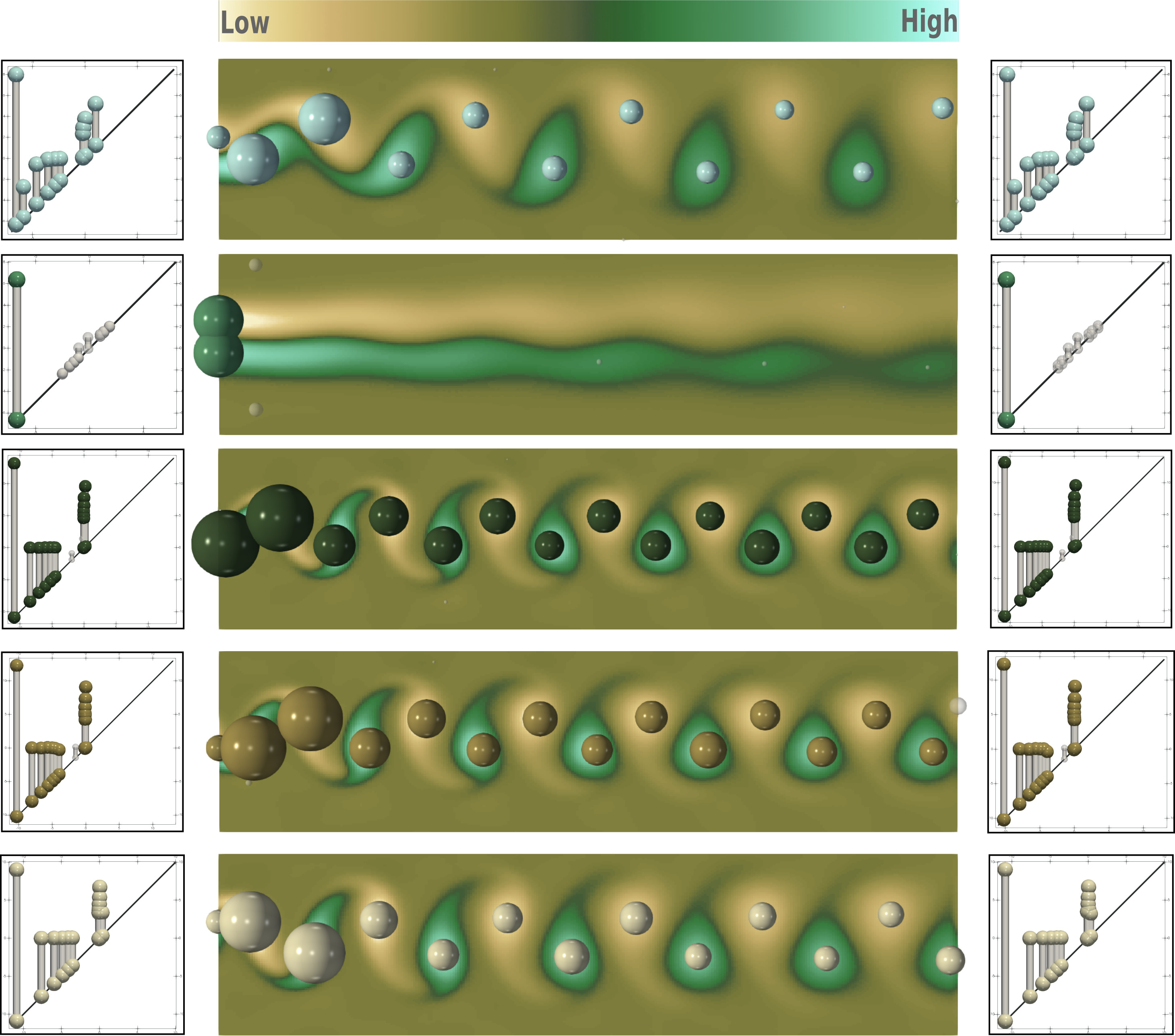
Figure 8: Clusters automatically identified by our topological clustering ($t_{max}$: 10 seconds). From top to bottom: pointwise mean of each cluster. Left: Centroids computed by our interruptible clustering algorithm. Right: Wasserstein barycenters of the clusters, computed by our progressive algorithm run until convergence. Differences are visually indistinguishable. Barycenter extrema are scaled in the domain by persistence (spheres).

5.3 Ensemble visual analysis with Topological Clustering

In the following, we systematically set a time constraint $t_{max}$ of 10 seconds. To facilitate the reading of the diagrams, each pair with a persistence smaller than $10\%$ of the function range is shown in transparent white, to help visually discriminate salient features from noise. Fig. 7 shows the clustering of the Gaussians ensemble by our approach. This synthetic ensemble exemplifies the motivation for the geometrical lifting introduced in Sec. 1.2(Sec. 1.2). The first and third clusters both contain a single Gaussian, resulting in diagrams with a single persistent feature, but located in drastically different areas of the domain $\mathscr{M}$. Thus, the diagrams of these two clusters would be indistinguishable for the clustering algorithm if geometrical lifting was not considered. If feature location is important for the application, our approach can be adjusted thanks to geometrical lifting (Sec. 1.2). For the Gaussians ensemble, this makes our clustering approach compute the correct clustering. Moreover, taking the geometry of the critical points into account allows us to represent in $\mathscr{M}$ the extrema involved in the Wasserstein barycenters (spheres, scaled by persistence, Fig. 7) which allows user to have a visual feedback in the domain of the features representative of the set of scalar fields. Geometrical lifting is particularly important in applications where feature location bears a meaning, such as the Isabel ensemble (Progressive Wasserstein Barycenters of Persistence Diagrams(f)). For this example, our clustering algorithm with geometrical lifting automatically identifies the right clusters, corresponding to the three states of the hurricane (formation, drift and landfall). For the remaining examples, geometrical lifting was not necessary ($\alpha=0$). For the Vortex Street ensemble (Fig. 8), our approach manages to automatically identify the correct clusters, precisely corresponding to the distinct viscosity regimes found in the ensemble. Note that the centroids computed by our topological clustering algorithm with a time constraint of 10 seconds (left) are visually indistinguishable from the Wasserstein barycenters of each cluster, computed after the fact with our progressive algorithm run until convergence (right). This indicates that the centroids provided by our topological clustering are reliable and can be used to visually represent the features of interest in the ensemble. In particular, for the Vortex Street example, these centroids enable the clear identification of the number and salience of the vortices: pairs which align horizontally and vertically respectively denote minima and maxima of flow vorticity, which respectively correspond to clockwise and counterclockwise vortices. Fig. 9 presents our results on the Starting Vortex, where our approach also automatically identifies the correct clustering, corresponding to two wing configurations. In this example, the difference in turbulence (number and strength of vortices) can be directly and visually read from the centroids returned by our algorithm (insets). Finally, Fig. 10 shows our results for the Sea Surface Height, where our topological clustering automatically identifies four clusters, corresponding to the four seasons: winter (top left), spring (top right), summer (bottom left), fall (bottom right). As shown in the insets, each season leads to a visually distinct centroid diagram. In this example, as diagrams are larger, differences between the interrupted centroids (left) and the converged barycenters (right) become noticeable. However, these differences only involve pairs of small persistence, whose contribution to the final clustering reveal negligible in practice.

Comparing with the approach from Favelier et al. [32], on the exact same data, we obtain similar qualitative results, with correct clusterings found on all data-sets. Performance-wise, our time-constrained approach finds the correct clustering within ten seconds for a large ensemble data-set such as Sea Surface Height (in addition to 35 seconds to compute the persistence diagrams) against several hundreds of seconds for the parallel persistence atlas approach. Overall, our approach provides the same clustering results than Favelier et al. [32]: the returned clusterings are correct for both approaches, for all of the above data sets. However, once the input persistence diagrams are available, our algorithm computes within a time constraint of ten seconds only, while the approach by Favelier et al. requires up to hundreds of seconds (on the same hardware) to compute intermediate representations (Persistence Maps) which are not needed in our work.

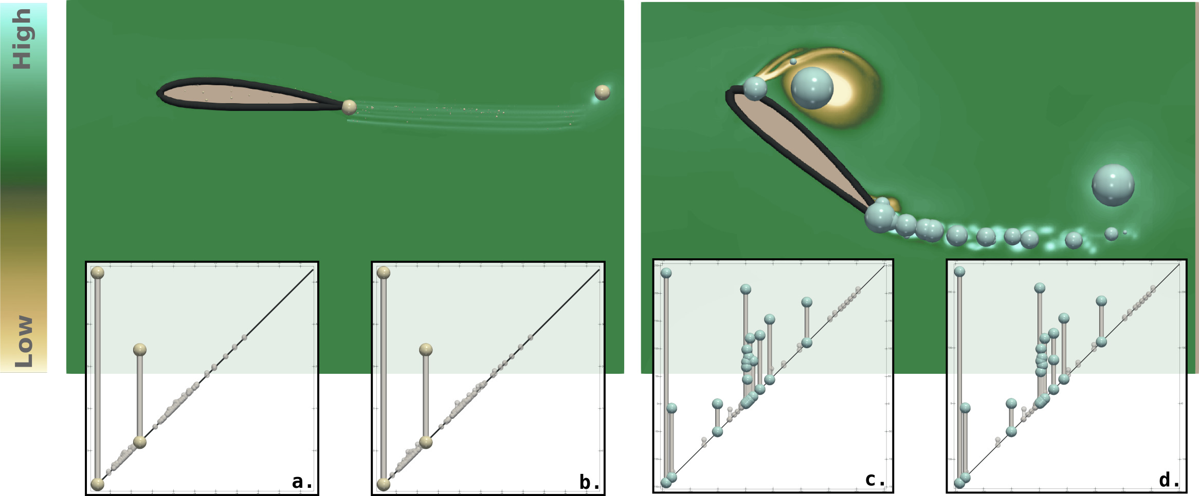
Figure 9: Clusters automatically identified by our topological clustering ($t_{max}:10s.$). Left insets (a, c): Centroids computed by our interruptible clustering algorithm. Right insets (b, d): Wasserstein barycenters of the clusters, computed by our progressive algorithm run until convergence. Differences are visually indistinguishable. Top: pointwise mean of each cluster. Barycenter extrema are scaled in the domain by persistence (spheres). Top: pointwise mean of each cluster, with barycenter extrema scaled by persistence (spheres).

5.4 Limitations

In our experiments, we focused on persistence diagrams which only involve extrema, as these often directly translate into features of interest in the applications. Although our approach can consider other types of persistence pairs (e.g. saddle-saddle pairs in 3D), from our experience, the interpretation of these structures is not obvious in practice and future work is needed to improve the understanding of these pairs in the applications. Thanks to the assignments computed by our algorithm, the extrema of the output barycenter can be embedded in the original domain (Fig. 7 to 10). However, in practice a given barycenter extremum can be potentially assigned with extrema which are distant from each other in the ensemble members, resulting in its placement at an in-between location which may not be relevant for the application. Regarding the Fréchet energy, our experiments confirm the proximity of our approximated barycenters to actual local minima (Fig. 4, Tab. 3). However, theoretical proximity bounds to these minima are difficult to formulate and we leave this for future work. However, aAlso, as it is the case for the original algorithm by Turner et al. [94], there is no guarantee that this solution is a global minimizerour solutions are global minimizers. For the clustering, we observed that the initialization of the $k$-means algorithm had a major impact on its outcome but we found that the $k$-means++ heuristic [21] provided excellent results in practice. Finally, when the geometrical location of features in the domain has a meaning for the applications, the geometrical lifting coefficient (Sec. 1.2) must be manually adjusted by the user on a per application basis, which involves a trial and error process. However, our interruptible approach greatly helps in this process, as users can perform such adjustments at interactive rates.

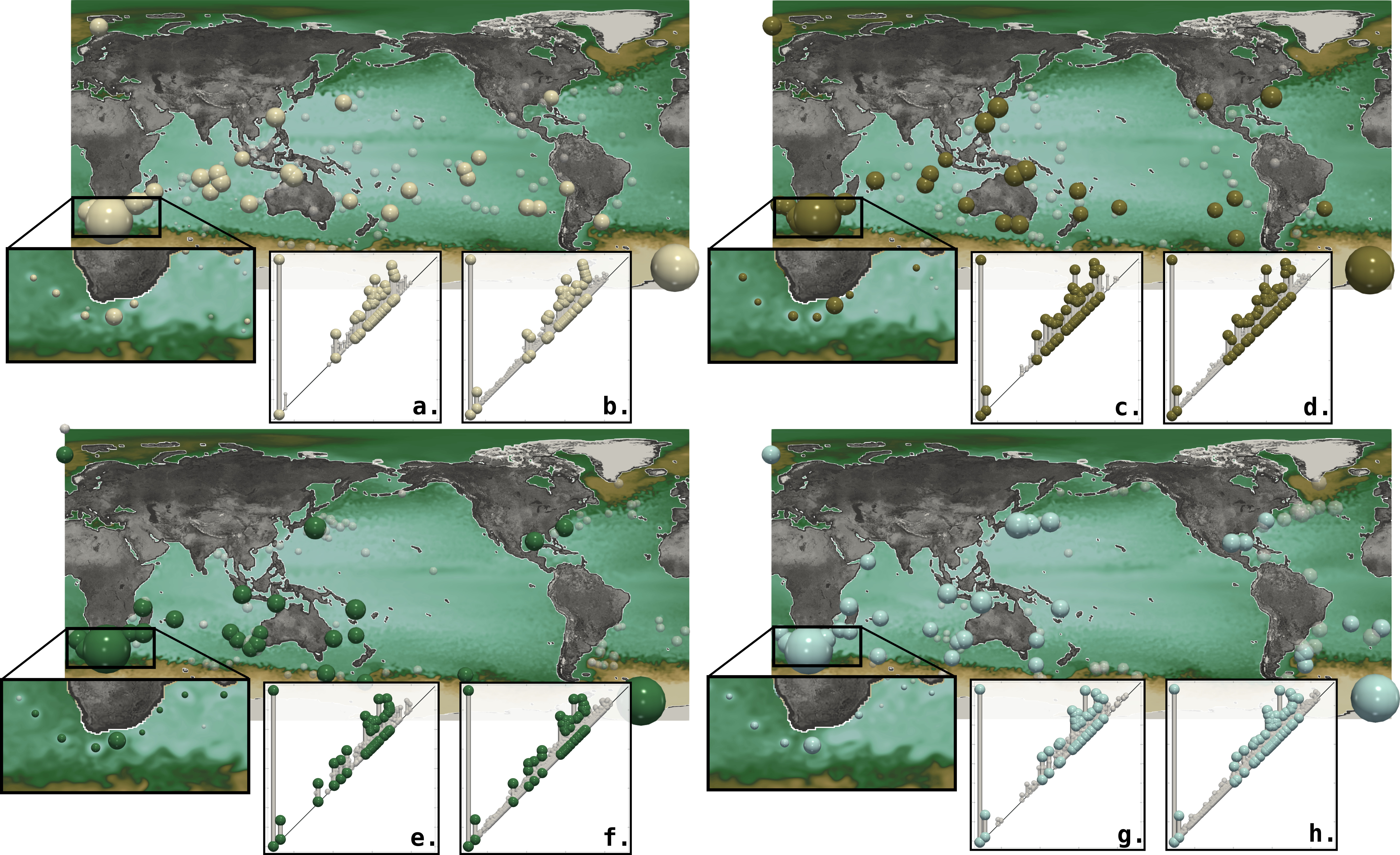
Figure 10: Clusters automatically identified by our topological clustering ($t_{max}:10s.$). From left to right, top to bottom: pointwise mean of each cluster. Barycenter extrema are embedded in the domain with spheres scaled by persistence. From left to right, top to bottom: pointwise mean of each cluster with barycenter extrema scaled by persistence (spheres). Left insets (a, c, e, g): Centroids computed by our interruptible clustering algorithm. Right insets (b, d, f, h): Wasserstein barycenters of the clusters, computed by our progressive algorithm run until convergence.

6 Conclusion

In this paper, we presented an algorithm for the progressive approximation of Wasserstein barycenters of Persistence diagrams, with applications to the visual analysis of ensemble data. Our approach takes advantage of previous results on the computation of Fréchet means for persistence diagrams [94], and revisits the fast approximation of Wasserstein distance [51] to induce progressivity. Our approach revisits efficient algorithms for Wasserstein distance approximation [12, 51] in order to specifically extend previous work on barycenter estimation [94]. Our experiments showed that our strategy drastically accelerates convergence and reported an order of magnitude speedup against previous work, while providing barycenters which are quantitatively comparable and visually similar. and visually comparable. The progressivity of our approach allowedallows for the definition of an interruptible algorithm, enabling the estimation of reliable barycenters within interactive times. We presented an application to the topological clustering of ensemble data, ensemble data clustering, where the obtained centroid diagrams provided key visual insights about the global feature trends of the ensemble.

A natural direction for future work is the extension of our framework to other topological abstractions, such as Reeb graphs or Morse-Smale complexes. However, the question of defining a relevant, and importantly, computable metric between these objects is still an active research debate. Our framework provides only approximations of Wasserstein barycenters. In the future, it would be useful to study the convergence of these approximations from a theoretical point of view. Although we have focused on scientific visualization applications, our framework can be used mostly as-is for persistence diagrams of more general data, such as filtrations of high dimensional point clouds. In that context, other applications than clustering will also be investigated. Moreover, we believe our progressive strategy for Wasserstein barycenters can also be used for more general inputs than persistence diagrams, such as generic point clouds, as long as an importance measure substituting persistence is available, which would significantly enlarge the spectrum of applications of the ideas presented in this paper.

- [1] ISO/IEC Guide 98-3:2008 uncertainty of measurement - part 3: Guide to the expression of uncertainty in measurement (GUM). 2008.
- [2] H. Adams, S. Chepushtanova, T. Emerson, E. Hanson, M. Kirby, F. Motta, R. Neville, C. Peterson, P. Shipman, and L. Ziegelmeier. Persistence Images: A Stable Vector Representation of Persistent Homology. Journal of Machine Learning Research, 2017.
- [3] K. Anderson, J. Anderson, S. Palande, and B. Wang. Topological data analysis of functional MRI connectivity in time and space domains. In MICCAI Workshop on Connectomics in NeuroImaging, 2018.
- [4] T. Athawale and A. Entezari. Uncertainty quantification in linear interpolation for isosurface extraction. IEEE Transactions on Visualization and Computer Graphics, 2013.
- [5] T. Athawale and C. R. Johnson. Probabilistic asymptotic decider for topological ambiguity resolution in level-set extraction for uncertain 2D data. IEEE Transactions on Visualization and Computer Graphics, 2019.
- [6] T. Athawale, E. Sakhaee, and A. Entezari. Isosurface visualization of data with nonparametric models for uncertainty. IEEE Transactions on Visualization and Computer Graphics, 2016.
- [7] U. Ayachit, A. C. Bauer, B. Geveci, P. O’Leary, K. Moreland, N. Fabian, and J. Mauldin. Paraview catalyst: Enabling in situ data analysis and visualization. In ISAV, 2015.
- [8] A. C. Bauer, H. Abbasi, J. Ahrens, H. Childs, B. Geveci, S. Klasky, K. Moreland, P. O’Leary, V. Vishwanath, B. Whitlock, and E. W. Bethel. In-situ methods, infrastructures, and applications on high performance computing platforms. Comp. Grap. For., 2016.
- [9] U. Bauer, X. Ge, and Y. Wang. Measuring distance between Reeb graphs. In Symp. on Comp. Geom., 2014.
- [10] U. Bauer, E. Munch, and Y. Wang. Strong equivalence of the interleaving and functional distortion metrics for Reeb graphs. In Symp. on Comp. Geom., 2015.
- [11] K. Beketayev, D. Yeliussizov, D. Morozov, G. H. Weber, and B. Hamann. Measuring the distance between merge trees. In TopoInVis. 2014.
- [12] D. P. Bertsekas. A new algorithm for the assignment problem. Mathematical Programming, 1981.
- [13] D. P. Bertsekas and D. Castañon. Parallel synchronous and asynchronous implementations of the auction algorithm. Parallel Computing, 1991.
- [14] H. Bhatia, A. G. Gyulassy, V. Lordi, J. E. Pask, V. Pascucci, and P.-T. Bremer. Topoms: Comprehensive topological exploration for molecular and condensed-matter systems. J. of Computational Chemistry, 2018.
- [15] H. Bhatia, S. Jadhav, P. Bremer, G. Chen, J. A. Levine, L. G. Nonato, and V. Pascucci. Flow visualization with quantified spatial and temporal errors using edge maps. IEEE Transactions on Visualization and Computer Graphics, 2012.
- [16] S. Biasotti, D. Giorgio, M. Spagnuolo, and B. Falcidieno. Reeb graphs for shape analysis and applications. Theoretical Computer Science, 2008.
- [17] G. Bonneau, H. Hege, C. Johnson, M. Oliveira, K. Potter, P. Rheingans, and T. Schultz”. Overview and state-of-the-art of uncertainty visualization. Mathematics and Visualization, 37:3–27, 2014.
- [18] P. Bremer, G. Weber, J. Tierny, V. Pascucci, M. Day, and J. Bell. Interactive exploration and analysis of large scale simulations using topology-based data segmentation. IEEE Transactions on Visualization and Computer Graphics, 2011.
- [19] H. Carr, J. Snoeyink, and U. Axen. Computing contour trees in all dimensions. In Symp. on Dis. Alg., 2000.
- [20] M. Carrière, M. Cuturi, and S. Oudot. Sliced Wasserstein Kernel for Persistence Diagrams. ICML, 2017.
- [21] M. E. Celebi, H. A. Kingravi, and P. A. Vela. A comparative study of efficient initialization methods for the k-means clustering algorithm. Expert Syst. Appl., 2013.
- [22] D. Cohen-Steiner, H. Edelsbrunner, and J. Harer. Stability of persistence diagrams. In Symp. on Comp. Geom., 2005.
- [23] M. Cuturi. Sinkhorn distances: Lightspeed computation of optimal transport. In NIPS. 2013.
- [24] M. Cuturi and A. Doucet. Fast computation of wasserstein barycenters. In ICML, 2014.
- [25] L. De Floriani, U. Fugacci, F. Iuricich, and P. Magillo. Morse complexes for shape segmentation and homological analysis: discrete models and algorithms. Comp. Grap. For., 2015.
- [26] P. Diggle, P. Heagerty, K.-Y. Liang, and S. Zeger. The Analysis of Longitudinal Data. Oxford University Press, 2002.
- [27] H. Edelsbrunner and J. Harer. Computational Topology: An Introduction. American Mathematical Society, 2009.
- [28] H. Edelsbrunner, J. Harer, and A. Zomorodian. Hierarchical Morse-Smale complexes for piecewise linear 2-manfiolds. Disc. Compu. Geom., 2003.
- [29] H. Edelsbrunner, D. Letscher, and A. Zomorodian. Topological persistence and simplification. Disc. Compu. Geom., 2002.
- [30] H. Edelsbrunner and E. P. Mucke. Simulation of simplicity: a technique to cope with degenerate cases in geometric algorithms. ACM Trans. on Graph., 1990.
- [31] C. Elkan. Using the triangle inequality to accelerate k-means. In ICML, 2003.
- [32] G. Favelier, N. Faraj, B. Summa, and J. Tierny. Persistence Atlas for Critical Point Variability in Ensembles. IEEE Transactions on Visualization and Computer Graphics, 2018.
- [33] G. Favelier, C. Gueunet, and J. Tierny. Visualizing ensembles of viscous fingers. In IEEE SciVis Contest, 2016.
- [34] F. Ferstl, K. Bürger, and R. Westermann. Streamline variability plots for characterizing the uncertainty in vector field ensembles. IEEE Transactions on Visualization and Computer Graphics, 2016.
- [35] F. Ferstl, M. Kanzler, M. Rautenhaus, and R. Westermann. Visual analysis of spatial variability and global correlations in ensembles of iso-contours. Comp. Grap. For., 2016.
- [36] D. Guenther, R. Alvarez-Boto, J. Contreras-Garcia, J.-P. Piquemal, and J. Tierny. Characterizing molecular interactions in chemical systems. IEEE Transactions on Visualization and Computer Graphics (Proc. of IEEE VIS), 2014.
- [37] C. Gueunet, P. Fortin, J. Jomier, and J. Tierny. Task-based Augmented Merge Trees with Fibonacci Heaps,. In IEEE LDAV, 2017.
- [38] D. Günther, J. Salmon, and J. Tierny. Mandatory critical points of 2D uncertain scalar fields. Computer Graphics Forum, 2014.
- [39] A. Gyulassy, P. Bremer, R. Grout, H. Kolla, J. Chen, and V. Pascucci. Stability of dissipation elements: A case study in combustion. Computer Graphics Forum, 2014.
- [40] A. Gyulassy, P. Bremer, and V. Pascucci. Shared-memory parallel computation of Morse-Smale complexes with improved accuracy. IEEE Transactions on Visualization and Computer Graphics, 2019.
- [41] A. Gyulassy, P. T. Bremer, B. Hamann, and V. Pascucci. A practical approach to Morse-Smale complex computation: Scalability and generality. IEEE Transactions on Visualization and Computer Graphics (Proc. of IEEE VIS), 2008.
- [42] A. Gyulassy, M. A. Duchaineau, V. Natarajan, V. Pascucci, E. Bringa, A. Higginbotham, and B. Hamann. Topologically clean distance fields. IEEE Transactions on Visualization and Computer Graphics (Proc. of IEEE VIS), 2007.
- [43] A. Gyulassy, D. Guenther, J. A. Levine, J. Tierny, and V. Pascucci. Conforming Morse-Smale complexes. IEEE Transactions on Visualization and Computer Graphics (Proc. of IEEE VIS), 2014.
- [44] A. Gyulassy, A. Knoll, K. Lau, B. Wang, P. Bremer, M. Papka, L. A. Curtiss, and V. Pascucci. Interstitial and interlayer ion diffusion geometry extraction in graphitic nanosphere battery materials. IEEE Transactions on Visualization and Computer Graphics (Proc. of IEEE VIS), 2015.
- [45] C. Heine, H. Leitte, M. Hlawitschka, F. Iuricich, L. De Floriani, G. Scheuermann, H. Hagen, and C. Garth. A survey of topology-based methods in visualization. Comp. Grap. For., 2016.
- [46] M. Hilaga, Y. Shinagawa, T. Kohmura, and T. L. Kunii. Topology matching for fully automatic similarity estimation of 3D shapes. In Proc. of ACM SIGGRAPH, 2001.
- [47] M. Hummel, H. Obermaier, C. Garth, and K. I. Joy. Comparative visual analysis of lagrangian transport in CFD ensembles. IEEE Transactions on Visualization and Computer Graphics, 2013.
- [48] C. R. Johnson and A. R. Sanderson. A next step: Visualizing errors and uncertainty. IEEE Computer Graphics and Applications, 2003.
- [49] L. Kantorovich. On the translocation of masses. AS URSS, 1942.
- [50] J. Kasten, J. Reininghaus, I. Hotz, and H. Hege. Two-dimensional time-dependent vortex regions based on the acceleration magnitude. IEEE Transactions on Visualization and Computer Graphics, 2011.
- [51] M. Kerber, D. Morozov, and A. Nigmetov. Geometry helps to compare persistence diagrams. ACM Journal of Experimental Algorithmics, 2016.
- [52] M. Kraus. Visualization of uncertain contour trees. In International Conference on Information Visualization Theory and Applications, 2010.
- [53] T. Lacombe, M. Cuturi, and S. Oudot. Large Scale computation of Means and Clusters for Persistence Diagrams using Optimal Transport. In NIPS, 2018.
- [54] D. E. Laney, P. Bremer, A. Mascarenhas, P. Miller, and V. Pascucci. Understanding the structure of the turbulent mixing layer in hydrodynamic instabilities. IEEE Transactions on Visualization and Computer Graphics (Proc. of IEEE VIS), 2006.
- [55] T. Liebmann and G. Scheuermann. Critical points of gaussian-distributed scalar fields on simplicial grids. Computer Graphics Forum (Proc. of EuroVis), 2016.
- [56] S. Lloyd. Least squares quantization in PCM. IEEE Transactions on Information Theory, 1982.
- [57] H.-C. H. M. Otto, T. Germer and H. Theisel. Uncertain 2D vector field topology. Comp. Graph. For., 29:347–356, 2010.
- [58] T. G. M. Otto and H. Theisel. Uncertain topology of 3D vector fields. Proc. of IEEE Pacific Vis, 2011.
- [59] A. Maceachren, A.Robinson, S. Hopper, S. Gardner, R. Murray, M. Gahegan, and E. Hetzler. Visualizing geospatial information uncertainty: What we know and what we need to know. Cartography and Geographic Information Science, 2005.
- [60] D. Maljovec, B. Wang, P. Rosen, A. Alfonsi, G. Pastore, C. Rabiti, and V. Pascucci. Topology-inspired partition-based sensitivity analysis and visualization of nuclear simulations. In Proc. of IEEE PacificVis, 2016.
- [61] M. Mirzargar, R. Whitaker, and R. Kirby. Curve boxplot: Generalization of boxplot for ensembles of curves. IEEE Transactions on Visualization and Computer Graphics, 2014.
- [62] G. Monge. Mémoire sur la théorie des déblais et des remblais. Académie Royale des Sciences de Paris, 1781.
- [63] D. Morozov. Dionysus. http://www.mrzv.org/software/dionysus, 2010. Accessed: 2019-03-01.
- [64] J. Munkres. Algorithms for the assignment and transportation problems. Journal of the Society for Industrial and Applied Mathematics, 1957.
- [65] A. T. Pang, C. M. Wittenbrink, and S. K. Lodha. Approaches to uncertainty visualization. The Visual Computer, 1997.
- [66] V. Pascucci, G. Scorzelli, P. T. Bremer, and A. Mascarenhas. Robust on-line computation of Reeb graphs: simplicity and speed. ACM Trans. on Graph., 2007.
- [67] C. Petz, K. Pöthkow, and H.-C. Hege. Probabilistic local features in uncertain vector fields with spatial correlation. Computer Graphics Forum, 2012.
- [68] T. Pfaffelmoser, M. Mihai, and R. Westermann. Visualizing the variability of gradients in uncertain 2D scalar fields. IEEE Transactions on Visualization and Computer Graphics, 2013.
- [69] T. Pfaffelmoser, M. Reitinger, and R. Westermann. Visualizing the positional and geometrical variability of isosurfaces in uncertain scalar fields. Computer Graphics Forum, 2011.
- [70] T. Pfaffelmoser and R. Westermann. Visualization of global correlation structures in uncertain 2D scalar fields. Comp. Grap. For., 2012.
- [71] K. Pöthkow and H.-C. Hege. Positional uncertainty of isocontours: Condition analysis and probabilistic measures. IEEE Transactions on Visualization and Computer Graphics, 2011.
- [72] K. Pöthkow and H.-C. Hege. Nonparametric models for uncertainty visualization. Comp. Grap. For., 2013.
- [73] K. Pöthkow, C. Petz, and H.-C. Hege. Approximate level-crossing probabilities for interactive visualization of uncertain isocontours. Int. J. Uncert. Quantif., 2013.
- [74] K. Pöthkow, B. Weber, and H.-C. Hege. Probabilistic marching cubes. In Computer Graphics Forum, 2011.
- [75] K. Potter, S. Gerber, and E. W. Anderson. Visualization of uncertainty without a mean. IEEE Computer Graphics and Applications, 2013.
- [76] K. Potter, A. Wilson, P. Bremer, D. Williams, C. Doutriaux, V. Pascucci, and C. R. Johnson. Ensemble-vis: A framework for the statistical visualization of ensemble data. In 2009 IEEE International Conference on Data Mining Workshops, 2009.
- [77] J. C. Potter K, Rosen P. From quantification to visualization: A taxonomy of uncertainty visualization approaches. IFIP Advances in Information and Communication Technology, 2012.
- [78] J. Reininghaus, S. Huber, U. Bauer, and R. Kwitt. A stable multi-scale kernel for topological machine learning. In IEEE CVPR, 2015.
- [79] B. Rieck, F. Sadlo, and H. Leitte. Topological machine learning with persistence indicator functions. In Proc. of TopoInVis, 2017.
- [80] L. Roy, P. Kumar, Y. Zhang, and E. Zhang. Robust and fast extraction of 3D symmetric tensor field topology. IEEE Transactions on Visualization and Computer Graphics, 2019.
- [81] H. Saikia, H. Seidel, and T. Weinkauf. Extended branch decomposition graphs: Structural comparison of scalar data. Computer Graphics Forum, 2014.
- [82] J. Sanyal, S. Zhang, J. Dyer, A. Mercer, P. Amburn, and R. Moorhead. Noodles: A tool for visualization of numerical weather model ensemble uncertainty. IEEE Transactions on Visualization and Computer Graphics, 2010.
- [83] S. Schlegel, N. Korn, and G. Scheuermann. On the interpolation of data with normally distributed uncertainty for visualization. IEEE Transactions on Visualization and Computer Graphics (Proc. of IEEE VIS), 2012.
- [84] I. SciVisContest. Simulation of the isabel hurricane. http://sciviscontest-staging.ieeevis.org/2004/data.html, 2004.
- [85] N. Shivashankar, P. Pranav, V. Natarajan, R. van de Weygaert, E. P. Bos, and S. Rieder. Felix: A topology based framework for visual exploration of cosmic filaments. IEEE Transactions on Visualization and Computer Graphics, 2016. http://vgl.serc.iisc.ernet.in/felix/index.html.
- [86] M. Soler, M. Plainchault, B. Conche, and J. Tierny. Lifted Wasserstein Matcher for Fast and Robust Topology Tracking. In IEEE Symposium on Large Data Analysis and Visualization, 2018.
- [87] J. Solomon, F. De Goes, G. Peyré, M. Cuturi, A. Butscher, A. Nguyen, T. Du, and L. Guibas. Convolutional wasserstein distances. ACM Transactions on Graphics, 2015.
- [88] T. Sousbie. The persistent cosmic web and its filamentary structure: Theory and implementations. Royal Astronomical Society, 2011. http://www2.iap.fr/users/sousbie/web/html/indexd41d.html.
- [89] A. Szymczak. Hierarchy of stable Morse decompositions. IEEE Transactions on Visualization and Computer Graphics, 2013.
- [90] D. M. Thomas and V. Natarajan. Detecting symmetry in scalar fields using augmented extremum graphs. IEEE Transactions on Visualization and Computer Graphics (Proc. of IEEE VIS), 2013.
- [91] D. M. Thomas and V. Natarajan. Multiscale symmetry detection in scalar fields by clustering contours. IEEE Transactions on Visualization and Computer Graphics (Proc. of IEEE VIS), 2014.
- [92] J. Tierny, G. Favelier, J. A. Levine, C. Gueunet, and M. Michaux. The Topology ToolKit. IEEE Transactions on Visualization and Computer Graphics (Proc. of IEEE VIS), 2017. https://topology-tool-kit.github.io/.
- [93] J. Tierny, A. Gyulassy, E. Simon, and V. Pascucci. Loop surgery for volumetric meshes: Reeb graphs reduced to contour trees. IEEE Transactions on Visualization and Computer Graphics (Proc. of IEEE VIS), 2009.
- [94] K. Turner, Y. Mileyko, S. Mukherjee, and J. Harer. Fréchet Means for Distributions of Persistence Diagrams. Disc. Compu. Geom., 2014.
- [95] R. T. Whitaker, M. Mirzargar, and R. M. Kirby. Contour boxplots: A method for characterizing uncertainty in feature sets from simulation ensembles. IEEE Transactions on Visualization and Computer Graphics, 2013.
- [96] K. Wu and S. Zhang. A contour tree based visualization for exploring data with uncertainty. International Journal for Uncertainty Quantification, 2013.