We propose a new highly flexible and tractable Bayesian approach to undertake variable selection in non-Gaussian regression models. It uses a copula decomposition for the joint distribution of observations on the dependent variable. This allows the marginal distribution of the dependent variable to be calibrated accurately using a nonparametric or other estimator. The family of copulas employed are ‘implicit copulas’ that are constructed from existing hierarchical Bayesian models widely used for variable selection, and we establish some of their properties. Even though the copulas are high-dimensional, they can be estimated efficiently and quickly using Markov chain Monte Carlo (MCMC). A simulation study shows that when the responses are non-Gaussian the approach selects variables more accurately than contemporary benchmarks. A real data example in the Web Appendix illustrates that accounting for even mild deviations from normality can lead to a substantial increase in accuracy. To illustrate the full potential of our approach we extend it to spatial variable selection for fMRI. Using real data, we show our method allows for voxel-specific marginal calibration of the magnetic resonance signal at over 6,000 voxels, leading to an increase in the quality of the activation maps.

1 Introduction

Bayesian approaches to selecting covariates in regression models are well established; see O’Hara and Sillanpää (2009) and Bottolo and Richardson (2010) for overviews. However, most work remains focused on Gaussian regression models, and extensions to the non-Gaussian case are limited. In particular, the importance of ‘marginal calibration’ in Bayesian variable (i.e. covariate) selection (BVS) is unexplored. Following Gneiting et al. (2007), by marginal calibration we mean the statistical consistency between the unconditional probability distribution of the dependent variable and its observations, with a more formal definition given by Gneiting et al. (2013, Defn. 2.6a). We address this here by proposing a new approach to BVS that is based on a copula decomposition for a vector of observations of length $n$ on the dependent variable. The impact of the covariates on the dependent variable is captured by the copula function only. This separates the task of selecting covariates from that of modeling the marginal distribution of the dependent variable; the latter of which can then be calibrated accurately. For the copula function we propose a new family of ‘implicit copulas’, which are constructed from existing popular Bayesian hierarchical regression models used for selecting covariates. By an implicit copula we mean the copula that is implicit in a multivariate distribution and obtained by inverting the usual expression of Sklar’s theorem as in Sec. 3.1 of Nelsen (2006). The result is a general and tractable approach that extends BVS to have an accurately calibrated margin for the dependent variable.

Low dimensional copulas are often used to capture dependence between multiple variables. Here the copula is used in a different way to capture the dependence between multiple observations on one dependent variable. The specification of this $n$-dimensional copula is the key ingredient of our method. To do so we consider a Gaussian linear model for $n$ observations on another dependent variable, which we call a ‘pseudo-response’ because it is not observed directly. Gaussian spike-and-slab priors with selection indicator variables $\gamma$ are employed for the coefficients. Integrating out these coefficients gives a Gaussian distribution for the pseudo-response vector conditional on the covariates and $\gamma$, and its implicit copula is a Gaussian copula (Song, 2000) with parameter matrix that is a function of the covariate values and $\gamma$. Finally, to obtain our copula family we mix this Gaussian copula over the scaling factor $g$ of the non-zero coefficients with respect to the different hyper-priors suggested by Liang et al. (2008). The resulting implicit copulas are mixtures of Gaussian copulas.

Because of its high dimension, it is difficult to evaluate our copula family directly. However, we show how to construct an MCMC sampler to undertake stochastic search variable selection (George and McCulloch, 1993), where the scaling factor $g$ is sampled using the Hamiltonian Monte Carlo (HMC) method of Hoffman and Gelman (2014). Careful use of matrix identities for the computations makes application of the method to high dimensions practical. A simulation study compares our approach to Gaussian BVS and the method of Rossell and Rubio (2018). It shows that accurate marginal calibration of the distribution the dependent variable—an intrinsic feature of our copula model—can result in more accurate covariate selection and predictive densities.

However, the main application of our approach is to spatial variable selection for functional magnetic resonance imaging (fMRI). In these studies a large vector of binary indicators signifies which voxels in a partition of the brain are active, so that it is large variable selection problem. We follow Smith et al. (2003), Smith and Fahrmeir (2007), Li and Zhang (2010) and Goldsmith et al. (2014) and use an Ising model as a prior to smooth the binary indicators spatially, but employ our copula model to allow for voxel-wise marginal calibration of the magnetic resonance (MR) signal. The neuroimaging literature suggests that accounting for such deviations from normality in the MR signal is important to obtain accurate activation maps (Eklund et al., 2017). Application of our approach to data from a visual experiment with $6192$ voxels shows this to be true here, and also produces much more accurate voxel-wise predictive distributions for the MR signal, as measured by the logarithmic scores. Importantly, the approach is both fast to implement and can be readily generalized, including to other binary random field priors for spatial smoothing of the binary indicators.

A number of other Bayesian approaches consider variable selection for non-Gaussian continuous-valued data. These include conditionally Gaussian models, where the disturbances follow a mixture of normals and/or data transformations of the dependent variable are considered, as in Smith and Kohn (1996) and Gottardo and Raftery (2009). Rossell and Rubio (2018) propose a BVS approach that allows for skewness and heavy tails by employing two-piece Gaussian and Laplace distributions for the errors. Chung and Dunson (2009) consider variable selection for a distributional regression model constructed through a probit stick-breaking process, Kundu and Dunson (2014) consider selection when the errors are modelled non-parametrically. Yu et al. (2013) propose variable selection in Bayesian quantile regression. However, none of these approaches fits our copula framework, nor ensure accurate calibration of the marginal distribution of the response. Sharma and Das (2018) proposed an alternative class of priors for regression coefficients based on copulas, and Kraus and Czado (2017) used a D-vine copula to capture flexibly the dependence between covariates and response in a regression model. However both use copulas in a very different way than suggested here and do not generalize existing BVS schemes as our approach does. Last, Klein and Smith (2019) construct implicit copulas from regularized smoothers, and our copula family extends these to variable selection.

The rest of this paper is structured as follows. Section 2 outlines our approach, including our proposed copula family. Section 3 details how to compute Bayesian inference, including the predictive densities and Bayes factors. Section 4 contains the simulation study, Section 5 extends the approach to spatial variable selection for fMRI data, and Section 6 concludes. A Web Appendix contains extensive additional material, including proofs, copula properties, details of the estimation algorithms, and the in-depth analysis of an additional regression dataset with $p=252$ correlated covariates.

2 Variable Selection in Regression using Copulas

2.1 Marginally calibrated variable selection

Consider a vector $\bm{Y}=(Y_{1},\ldots,Y_{n})^{\prime}$ of $n$ realisations on a continuous dependent variable, along with an $n\times p$ design matrix $\bm{X}$ for $p$ regression covariates. Bayesian approaches to variable selection usually proceed by introducing a vector of binary indicator variables $\text{\boldmath$\gamma$}=(\gamma_{1},\ldots,\gamma_{p})^{\prime}$, such that the $j$th covariate is included in the regression if $\gamma_{j}=1$, and excluded if $\gamma_{j}=0$. When the dependent variable is non-Gaussian, the most common approach is to consider non-Gaussian distributions for the disturbance to a linear model; see Kundu and Dunson (2014), Rossell and Rubio (2018) and references therein. Thus, a non-Gaussian distribution is selected for $Y_{i}$, conditional on $\bm{X}$ and $\gamma$. In this paper we suggest an alternative approach based on copulas that allows the marginal distribution of $Y_{i}$, unconditional on $\bm{X}$ and $\gamma$, to be chosen. We model the joint density of $\bm{Y}|\bm{X},\text{\boldmath$\gamma$}$ as

$$p(\text{\boldmath$y$}|\bm{X},\text{\boldmath$\gamma$})=c_{\mbox{\tiny BVS}}(\text{\boldmath$u$}|\bm{X},\text{\boldmath$\gamma$})\prod_{i=1}^{n}p_{Y}(y_{i})\,,$$ (1)

where $\text{\boldmath$y$}=(y_{1},\ldots,y_{n})^{\prime}$, $\text{\boldmath$u$}=(u_{1},\ldots,u_{n})^{\prime}$, $u_{i}=F_{Y}(y_{i})$ and the distribution of $Y_{i}$ is assumed to be marginally invariant with respect to $\bm{X}$ and $\gamma$, with density $p_{Y}$ and distribution function $F_{Y}$. The impact of the covariate values $\bm{X}$ and model indicators $\gamma$ on $\bm{Y}$ jointly is captured through the copula with density $c_{\mbox{\tiny BVS}}$, which is a function of $\bm{X}$ and $\gamma$. For this we use the copula proposed in Section 2.2 below.

A major advantage of employing (1) is that it separates the modeling of the marginal distribution $F_{Y}$ of the data, from the task of selecting the covariates. Therefore, $F_{Y}$ can be calibrated accurately, and we model it non-parametrically in our work. Variable selection is based on the posterior distribution of $\gamma$, which is given by

$$p(\text{\boldmath$\gamma$}|\bm{X},\text{\boldmath$y$})\propto p(\text{\boldmath$y$}|\bm{X},\text{\boldmath$\gamma$})p(\text{\boldmath$\gamma$})\propto c_{\mbox{\tiny BVS}}(\text{\boldmath$u$}|\bm{X},\text{\boldmath$\gamma$})p(\text{\boldmath$\gamma$})\,,$$ (2)

with model prior $p(\text{\boldmath$\gamma$})$. A major aim of this paper is to show that adopting (1) with our proposed copula provides a very general, but tractable, approach to undertaking variable selection and model averaging for non-Gaussian regression data.

We make three remarks concerning the appropriateness of the decomposition at (1). First, regression models are usually specified conditional on parameters for the mean, variance and possibly other moments. In contrast, the expressions above are unconditional on such parameters. We show in Part B of the Web Appendix that when also conditioning on additional model parameters introduced below in Section 2.2, the distribution of $Y_{i}$ is a function of the covariates, as is expected in a regression model. Second, we show in Part A of the Web Appendix that in a Gaussian linear regression model with a zero mean g-prior for the regression coefficients, the margin of $Y_{i}$ with the coefficients and error variance integrated out, is asymptotically independent of $\bm{X}$. Third, the predictive density arising from the copula model at (1) is a function of the covariate values and indicator variables $\gamma$. To see this, consider a new realization $Y_{n+1}$, with a $p\times 1$ vector of covariate values $\text{\boldmath$x$}_{n+1}$. Let $\bm{X}^{+}=[\bm{X}^{\prime}|\text{\boldmath$x$}_{n+1}]^{\prime}$ and $\text{\boldmath$u$}^{+}=(\text{\boldmath$u$}^{\prime},F_{Y}(y_{n+1}))^{\prime}$, then from (1), $Y_{n+1}$ has predictive density

$$p(y_{n+1}|\bm{X}^{+},\text{\boldmath$\gamma$},\text{\boldmath$y$})=\frac{p(y_{n+1},\text{\boldmath$y$}|\bm{X}^{+},\text{\boldmath$\gamma$})}{p(\text{\boldmath$y$}|\bm{X},\text{\boldmath$\gamma$})}=\frac{c_{\mbox{\tiny BVS}}(\text{\boldmath$u$}^{+}|\bm{X}^{+},\text{\boldmath$\gamma$})}{c_{\mbox{\tiny BVS}}(\text{\boldmath$u$}|\bm{X},\text{\boldmath$\gamma$})}p_{Y}(y_{n+1})\,.$$ (3)

This is a function of the observed values of all the covariates and $\gamma$. Moreover, marginalizing over the posterior of $\gamma$ gives the posterior predictive density for $Y_{n+1}|\bm{X}^{+},\text{\boldmath$y$}$ as

$$p(y_{n+1}|\bm{X}^{+},\text{\boldmath$y$})=\sum_{\text{\boldmath$\gamma$}}p(y_{n+1}|\bm{X}^{+},\text{\boldmath$\gamma$},\text{\boldmath$y$})p(\text{\boldmath$\gamma$}|\bm{X},\text{\boldmath$y$})\,.$$ (4)

This forms the basis of the predictive distribution of $Y_{n+1}$ from the copula model, and we give a computationally tractable expression for (4) in Section 3.2.2.

2.2 Variable selection copula

Key to our approach is the specification of our proposed copula with density $c_{\mbox{\tiny BVS}}$. To derive this, consider the linear model

$${\widetilde{\text{\boldmath$Z$}}}=\bm{X}_{\gamma}\text{\boldmath$\beta$}_{\gamma}+\text{\boldmath$\varepsilon$}\,,$$ (5)

where $\widetilde{\text{\boldmath$Z$}}=(\tilde{Z}_{1},\ldots,\tilde{Z}_{n})^{\prime}$, $\bm{X}_{\gamma}$ is an $n\times q_{\gamma}$ sub-matrix of $\bm{X}$ that comprises the columns of $\bm{X}$ where $\gamma_{j}=1$ (so $q_{\gamma}=\sum_{j=1}^{p}\gamma_{j}$), $\text{\boldmath$\beta$}_{\gamma}$ are the corresponding regression coefficients, and $\text{\boldmath$\varepsilon$}\sim\operatorname{N}(\mathbf{0},\sigma^{2}\text{\boldmath$I$})$. We refer to $\widetilde{\bm{Z}}$ as a vector of observations on a ‘pseudo-response’, because it is not observed directly in our model. Following Smith and Kohn (1996); George and McCulloch (1997); Liang et al. (2008) and many others, the conjugate g-prior $\text{\boldmath$\beta$\unboldmath${}_{\gamma}$}|\bm{X},\sigma^{2},\text{\boldmath$\gamma$},g\sim\operatorname{N}(\bm{0},g\sigma^{2}(\text{$\bm{X}_{\gamma}$}^{\prime}\text{$\bm{X}_{\gamma}$})^{-1})$, $g>0$, is used for the non-zero coefficients. Its conjugacy and scaling prove attractive features for constructing the variable selection copula.

To construct the variable selection copula, we first extract the implicit copula of the distribution of $\widetilde{\bm{Z}}$ conditional on $\bm{X},\text{\boldmath$\gamma$},g,\sigma^{2}$, but with $\text{\boldmath$\beta$}_{\gamma}$ integrated out. This is $\widetilde{\text{\boldmath$Z$}}|\bm{X},\text{\boldmath$\gamma$},g,\sigma^{2}\sim N(\bm{0};\bf{\Omega})$, where

$$\bm{\Omega}=\sigma^{2}\left(\text{\boldmath$I$}-\tfrac{g}{1+g}\text{$\bm{X}_{\gamma}$}(\text{$\bm{X}_{\gamma}$}^{\prime}\text{$\bm{X}_{\gamma}$})^{-1}\text{$\bm{X}_{\gamma}$}^{\prime}\right)^{-1}=\sigma^{2}(\text{\boldmath$I$}+g\text{$\bm{X}_{\gamma}$}(\text{$\bm{X}_{\gamma}$}^{\prime}\text{$\bm{X}_{\gamma}$})^{-1}\text{$\bm{X}_{\gamma}$}^{\prime})\,,$$

which follows from integrating out $\text{\boldmath$\beta$}_{\gamma}$ as a normal, and applying the Woodbury formula. The implicit copula is the Gaussian copula (Song, 2000), with parameter matrix equal to the correlation $\bm{R}$ of the distribution, and density $c_{\mbox{\tiny Ga}}(\text{\boldmath$u$};\bm{R})=|\bm{R}|^{-1/2}\exp\left(-\frac{1}{2}\text{\boldmath$z$}^{\prime}(\bm{R}^{-1}-\text{\boldmath$I$})\text{\boldmath$z$}\right)\,,$ where $\text{\boldmath$z$}=(\Phi^{-1}_{1}(u_{1}),\ldots,\Phi^{-1}_{1}(u_{n}))^{\prime}$ and $\Phi_{1}$ is the standard normal distribution function. To derive $\bm{R}$ we standardize $\mathbf{\Omega}$ by the variances

$$\operatorname{Var}(\tilde{Z}_{i}|\bm{X},\text{\boldmath$\gamma$},g,\sigma^{2})=\sigma^{2}(1+g\text{$\bm{x}_{\gamma,i}$}^{\prime}(\text{$\bm{X}_{\gamma}$}^{\prime}\text{$\bm{X}_{\gamma}$})^{-1}\text{$\bm{x}_{\gamma,i}$})\equiv\sigma^{2}s_{i}^{-2}\,,\mbox{ for}\,\,i=1,\ldots,n\,,$$

where $\text{$\bm{x}_{\gamma,i}$}^{\prime}$ is the $i$th row of $\bm{X}_{\gamma}$. Let $\bm{S}_{\gamma}\equiv\bm{S}(\bm{X},\text{\boldmath$\gamma$},g)=\operatorname{diag}(s_{1},\ldots,s_{n})$, then

$$\bm{R}\equiv\bm{R}(\bm{X},\text{\boldmath$\gamma$},g)=\frac{1}{\sigma^{2}}\bm{S}_{\gamma}\mathbf{\Omega}\bm{S}_{\gamma}=\bm{S}_{\gamma}\left(\text{\boldmath$I$}+g\text{$\bm{X}_{\gamma}$}(\text{$\bm{X}_{\gamma}$}^{\prime}\text{$\bm{X}_{\gamma}$})^{-1}\text{$\bm{X}_{\gamma}$}^{\prime}\right)\bm{S}_{\gamma}\,.$$ (6)

Note that the location and scale of $\widetilde{\bm{Z}}$ are unidentified in its copula, and $\bm{R}$ is not a function of $\sigma^{2}$. Therefore, without loss of generality, we set $\sigma^{2}=1$ and do not include an intercept in $\bm{X}$. We stress here that this does not mean the observational data $Y_{i}$ has zero mean or fixed scale, which is instead captured through $F_{Y}$ in (1).

Table 1: Summary of the one-to-one transformations between the dependent variable $Y_{i}$, copula variable $U_{i}$ specified in Section 2, and the standardized pseudo-response $Z_{i}=\frac{s_{i}}{\sigma}\tilde{Z}_{i}$ specified in Section 3.1. Also given are the joint densities of $\bm{Y}=(Y_{1},\ldots,Y_{n})^{\prime}$, $\bm{U}=(U_{1},\ldots,U_{n})^{\prime}$ and $\bm{Z}=(Z_{1},\ldots,Z_{n})^{\prime}$ conditioning on $\bm{X},\text{\boldmath$\gamma$}$ and with/without $g$. Above, $\text{\boldmath$y$}=(y_{1},\ldots,y_{n})^{\prime}$, $\text{\boldmath$u$}=(u_{1},\ldots,u_{n})^{\prime}$, $\text{\boldmath$z$}=(z_{1},\ldots,z_{n})^{\prime}$ and the $n\times n$ correlation matrix $\bm{R}\equiv\bm{R}(\bm{X},\text{\boldmath$\gamma$},g)$ is specified at (6).

	Observed Data	Copula Data	Standardized Pseudo-data
Variable	$Y_{i}$	$U_{i}=F_{Y}(Y_{i})$	$Z_{i}=\Phi_{1}^{-1}(U_{i})$
Domain	$\mathds{R}$	$[0,1]$	$\mathds{R}$
Marginal distribution	$F_{Y}$	Uniform	Standard Normal
Joint density	$p(\text{\boldmath$y$}|\bm{X},\text{\boldmath$\gamma$},g)=\phi(\text{\boldmath$z$};\mathbf{0},\bm{R})$	$p(\text{\boldmath$u$}|\bm{X},\text{\boldmath$\gamma$},g)=c_{\mbox{\tiny{Ga}}}(\text{\boldmath$u$}|\bm{X},\text{\boldmath$\gamma$},g)$	$p(\text{\boldmath$z$}|\bm{X},\text{\boldmath$\gamma$},g)=\phi(\text{\boldmath$z$};\mathbf{0},\bm{R})$
conditional on $\bm{X},\text{\boldmath$\gamma$},g$	$\times\prod_{i=1}^{n}\frac{p_{Y}(y_{i})}{\phi_{1}(z_{i})}$
Joint density	$p(\text{\boldmath$y$}|\bm{X},\text{\boldmath$\gamma$})=c_{\mbox{\tiny{BVS}}}(\text{\boldmath$u$}|\bm{X},\text{\boldmath$\gamma$})$	$p(\text{\boldmath$u$}|\bm{X},\text{\boldmath$\gamma$})=c_{\mbox{\tiny{BVS}}}(\text{\boldmath$u$}|\bm{X},\text{\boldmath$\gamma$})$	$p(\text{\boldmath$z$}|\bm{X},\text{\boldmath$\gamma$})=\int\phi(\text{\boldmath$z$};\mathbf{0},\bm{R})p(g)\mathrm{d}g$
conditional on $\bm{X},\text{\boldmath$\gamma$}$	$\times\prod_{i=1}^{n}p_{Y}(y_{i})$

Finally, we mix over $g$ with respect to its prior $p(g)$ to obtain the variable selection copula as a continuous mixture of Gaussian copulas, as defined below.

Definition 1

Let $C_{\mbox{\tiny Ga}}$ and $c_{\mbox{\tiny Ga}}$ be the Gaussian copula function and density, respectively. Then if $\widetilde{\bm{Z}}$ follows the linear model at (5), with the g-prior for $\bm{\beta}_{\gamma}$, and $p(g)$ is a proper density for $g>0$, then we call $C_{\mbox{\tiny BVS}}(\bm{u}|\bm{X},\text{\boldmath$\gamma$})=\int C_{\mbox{\tiny Ga}}(\bm{u};\bm{R}(\bm{X},\text{\boldmath$\gamma$},g))p(g)\mathrm{d}g$ a variable selection copula, with density function

$$c_{\mbox{\tiny BVS}}(\bm{u}|\bm{X},\text{\boldmath$\gamma$})=\int c_{\mbox{\tiny Ga}}(\bm{u};\bm{R}(\bm{X},\text{\boldmath$\gamma$},g))p(g)\mathrm{d}g\,.$$

It is straightforward to show the function $C_{\mbox{\tiny BVS}}(\bm{u}|\bm{X},\text{\boldmath$\gamma$})$ is a well-defined copula function.

Table 1 depicts the transformations underlying the construction of $C_{\mbox{\tiny BVS}}$. Part C of the Web Appendix gives some properties of $C_{\mbox{\tiny BVS}}$. We consider the three priors discussed by Liang et al. (2008) for $g$, and a point mass, as listed below:

• Hyper-$g$ prior: with density $p(g)=\tfrac{a-2}{2}(1+g)^{-a/2}$, which is proper for $a>2$. This implies a beta prior on the shrinkage factor $g/(1+g)\sim\mbox{Beta}(1,0.5a-1)$, and we set $a=4$ leading to a uniform prior on this factor.

• Hyper-$g/n$ prior: with density $p(g)=\tfrac{a-2}{2n}(1+g/n)^{-a/2}$ and $a=4$.

• Zellner-Siow prior: with density $p(g)=\tfrac{\sqrt{n/2}}{\Gamma(1/2)}c^{-3/2}\exp(-n/(2g))$.

• Point mass prior: We also consider fixing $g=100$ and $g=n$ for comparison.

While computing the integral over $g$ in Defn. 1 is possible using numerical methods, in general it is difficult to evaluate $C_{\mbox{\tiny BVS}}$ or $c_{\mbox{\tiny BVS}}$ directly because $\bm{R}(\bm{X},\text{\boldmath$\gamma$},g)$ is an $n$-dimensional matrix. Instead, we generate $g$ as part of an MCMC scheme, as discussed in Section 3. We use the popular prior $p(\text{\boldmath$\gamma$})=B(p-q_{\gamma}+1,q_{\gamma}+1)$, where $B$ is the beta function, which implies $p(q_{\gamma})=1/(p+1)$.

3 Estimation and Inference

Estimation of (1) requires estimation of both the marginal $F_{Y}$ and copula parameters $\gamma$. It is common to use two-stage estimators, where $F_{Y}$ is estimated first, followed by $\gamma$, because they are much faster and often involve only a minor loss of efficiency (Joe, 2005). Grazian and Liseo (2017) and Klein and Smith (2019) integrate out uncertainty for $F_{Y}$ using a Bayesian non-parametric estimator, but find that this does not improve the accuracy of inference meaningfully, as we also demonstrate in an empirical example in Part F of the Web Appendix. Therefore, we adopt a two-stage estimator, and use the adaptive kernel density estimator (KDE) of Shimazaki and Shinomoto (2010) to estimate $F_{Y}$.

3.1 Posterior evaluation

We follow George and McCulloch (1993) and evaluate the posterior of $\gamma$ using MCMC. However, direct computation of the posterior mass at (2) is slow because computing $c_{\mbox{\tiny BVS}}$ requires integration over $g$, so we generate $g$ as part of the MCMC scheme. To implement the sampler we follow Klein and Smith (2019) and express the likelihood conditional on $g$ in closed form by transforming to the (normalized) pseudo-response as follows. Let $\bm{Z}=(Z_{1},\ldots,Z_{n})^{\prime}=\frac{1}{\sigma}\bm{S}_{\gamma}\widetilde{\bm{Z}}$, where $\widetilde{\bm{Z}}$ is the pseudo-response at (5), then it follows from Section 2.2 that $\bm{Z}|\bm{X},\text{\boldmath$\gamma$},g\sim N(\bm{0},\bm{R}(\bm{X},\text{\boldmath$\gamma$},g))$. Moreover, $Y_{i}$ can be expressed in terms of $Z_{i}$ as $Y_{i}=F_{Y}^{-1}(\Phi_{1}(Z_{i}))$, so that by a change of variables from $\bm{Y}$ to $\bm{Z}$,

$$p(\text{\boldmath$y$}|\bm{X},\text{\boldmath$\gamma$},g)=p(\text{\boldmath$z$}|\bm{X},\text{\boldmath$\gamma$},g)\prod_{i=1}^{n}\frac{p_{Y}(y_{i})}{\phi_{1}(z_{i})}=\phi(\text{\boldmath$z$};\mathbf{0},\bm{R})\prod_{i=1}^{n}\frac{p_{Y}(y_{i})}{\phi_{1}(z_{i})}\,,$$ (7)

where the Jacobian of the transformation is $|\frac{d\bm{z}}{d\bm{y}}|=\prod_{i=1}^{n}\frac{p_{Y}(y_{i})}{\phi_{1}(z_{i})}$, $\phi_{1}$ is the standard normal density, and $\phi(\text{\boldmath$z$};\bm{0},\bm{R})$ is the density of a $N(\bm{0},\bm{R})$ distribution.

While all the terms in the right-hand side of (7) are known, the $n\times n$ matrix $\bm{R}$ cannot be computed directly for large $n$. To evaluate the posterior, we employ the following sampler.

MCMC Sampler
At each sweep:
Step 1. Randomly partition $\gamma$ into pairs of elements.
Step 2. For each pair $(\gamma_{i},\gamma_{j})$, generate from $p(\gamma_{i},\gamma_{j}|\{\text{\boldmath$\gamma$}\backslash\gamma_{i},\gamma_{j}\},\bm{X},g,\text{\boldmath$y$})$.
Step 3. Generate from $p(g|\bm{X},\text{\boldmath$\gamma$},\text{\boldmath$y$})$ using Hamiltonian Monte Carlo.

In forming the partition in Step 1, if $p$ is odd-valued one element is simply selected twice, so that pairs of elements $(\gamma_{i},\gamma_{j})$ are always generated in Step 2. Sampling pairs of elements of $\gamma$ in random order helps to improve mixing of the chain. To implement Step 2, from (7) the joint posterior of the indicators is

$$p(\bm{\gamma}|\bm{X},g,\bm{y}) \propto p(\text{\boldmath$y$}|\bm{X},\text{\boldmath$\gamma$},g)p(\bm{\gamma})\propto\phi(\text{\boldmath$z$};\bm{0},\bm{R}(\bm{X},\text{\boldmath$\gamma$},g))p(\bm{\gamma})$$

$$\propto |\bm{R}(\bm{X},\text{\boldmath$\gamma$},g)|^{-1/2}\exp\left\{-\frac{1}{2}\left(\text{\boldmath$z$}^{\prime}\bm{R}(\bm{X},\text{\boldmath$\gamma$},g)^{-1}\text{\boldmath$z$}\right)\right\}p(\text{\boldmath$\gamma$})\equiv A(\gamma_{i},\gamma_{j})\,.$$

Simulating $(\gamma_{i},\gamma_{j})$ involves computing $A$ for the four possible configurations
${\cal S}\equiv\{(0,0),(0,1),(1,0),(1,1)\}$, and then setting

$$p((\gamma_{i},\gamma_{j})|\{\text{\boldmath$\gamma$}\backslash(\gamma_{i},\gamma_{j})\},\bm{X},g,\text{\boldmath$y$})=\frac{1}{1+h}\,,\;\;h=\sum_{(\tilde{\gamma}_{i},\tilde{\gamma}_{j})\in\{{\cal S}\backslash(\gamma_{i},\gamma_{j})\}}\frac{A(\tilde{\gamma}_{i},\tilde{\gamma}_{j})}{A(\gamma_{i},\gamma_{j})}\,,$$ (8)

where all ratios are computed on the logarithmic scale. Fast computation of $A$ for the four configurations in ${\cal S}$ can be done using a number of matrix identities; see Part D of the Web Appendix, where at no stage is the full $n\times n$ matrix $\bm{R}$ computed directly.

Generating $g$ at Step 3 uses an HMC step for $\tilde{g}=\log(g)$. We use a variant of the leapfrog integrator of Neal (2011) with the dual averaging approach of Hoffman and Gelman (2014). This requires computation of $\log(p(\tilde{g}|\bm{X},\text{\boldmath$\gamma$},\text{\boldmath$y$}))$ up to an additive constant, and its derivative. Part D of the Web Appendix derives analytical expressions for these, and outlines the HMC step in greater detail. We found that the sampler above works well in our applications, although a referee highlighted that such samplers may mix poorly for large $p$, in which case adaptive non-Markov samplers as in Griffin et al. (2017) may be preferable.

3.2 Inference

The sampler above produces Monte Carlo draws $\{\text{\boldmath$\gamma$}^{[k]},g^{[k]};k=1,\ldots,K\}$ from the posterior $p(\text{\boldmath$\gamma$},g|\bm{X},\text{\boldmath$y$})$ and is used to compute posterior estimates as detailed below.

3.2.1 Variable selection

Variables can be selected using the marginal posteriors, which are estimated as

$$\mbox{Pr}(\gamma_{i}=1|\bm{X},\text{\boldmath$y$})\approx\frac{1}{K}\sum_{k=1}^{K}\mbox{Pr}(\gamma_{i}=1|\{\text{\boldmath$\gamma$}^{[k]}\backslash(\gamma_{i},\gamma_{j})\},\bm{X},g^{[k]},\text{\boldmath$y$})\,.$$

To evaluate the term in this summation, at Step 2 of the sampler for the single pair $(\gamma_{i},\gamma_{j})$ that contains $\gamma_{i}$, the following is computed

$$\mbox{Pr}(\gamma_{i}=1|\{\text{\boldmath$\gamma$}\backslash(\gamma_{i},\gamma_{j})\},\bm{X},g,\text{\boldmath$y$})=\frac{A(1,0)+A(1,1)}{A(0,0)+A(1,0)+A(0,1)+A(1,1)}\,,$$

where the four values of the bivariate function $A(\gamma_{i},\gamma_{j})$ are already computed at (8).

3.2.2 Predictive density

In general, direct evaluation of the predictive density of a new observation $Y_{n+1}$ with covariates $\text{\boldmath$x$}_{n+1}$ at (3) is infeasible because evaluating $c_{\mbox{\tiny BVS}}$ is also. However, the posterior predictive density at (4) can still be evaluated as:

$$p(y_{n+1}|\bm{X}^{+},\text{\boldmath$y$})=\sum_{\text{\boldmath$\gamma$}}\int\int p(y_{n+1}|\bm{X}^{+},\text{\boldmath$\beta$}_{\gamma},\text{\boldmath$\gamma$},g,\text{\boldmath$y$})p(\text{\boldmath$\beta$}_{\gamma},\text{\boldmath$\gamma$},g|\bm{X},\bm{y})\mathrm{d}(\text{\boldmath$\beta$}_{\gamma},g)\,.$$ (9)

The predictive density inside the integrals above can obtained by considering a change of variables from $Y_{n+1}$ to $Z_{n+1}=\Phi_{1}^{-1}(F_{Y}(Y_{n+1}))$, with Jacobian $\frac{p_{Y}(y_{n+1})}{\phi_{1}(z_{n+1})}$, as

$$p(y_{n+1}|\bm{X}^{+},\text{\boldmath$\beta$}_{\gamma},\text{\boldmath$\gamma$},g,\text{\boldmath$y$})=p(z_{n+1}|\bm{X}^{+},\text{\boldmath$\beta$}_{\gamma},g,\text{\boldmath$\gamma$},\text{\boldmath$z$})\frac{p_{Y}(y_{n+1})}{\phi_{1}(z_{n+1})}\,.$$

From (5), $\tilde{Z}_{n+1}|\text{\boldmath$x$}_{\gamma,i},\text{\boldmath$\beta$}_{\gamma},\text{\boldmath$\gamma$},g\sim N(\text{\boldmath$x$}_{\gamma,{n+1}}^{\prime}\text{\boldmath$\beta$}_{\gamma},\sigma^{2})$ independently when conditioning on $\text{\boldmath$\beta$}_{\gamma}$ (whereas the elements of $\widetilde{\bm{Z}}$ are dependent unconditional on $\text{\boldmath$\beta$}_{\gamma}$). Then, because $Z_{n+1}=\frac{s_{n+1}}{\sigma}\tilde{Z}_{n+1}$,

$$p(y_{n+1}|\bm{X}^{+},\text{\boldmath$\beta$}_{\gamma},\text{\boldmath$\gamma$},g,\text{\boldmath$y$})=\frac{1}{s_{n+1}}\phi_{1}\left(\frac{z_{n+1}-s_{n+1}\text{\boldmath$x$}_{\gamma,n+1}^{\prime}\text{\boldmath$\beta$}_{\gamma}}{s_{n+1}}\right)\frac{p_{Y}(y_{n+1})}{\phi_{1}(z_{n+1})}\,,$$ (10)

where $s_{n+1}=(1+g\text{\boldmath$x$}_{\gamma,n+1}^{\prime}(\text{$\bm{X}_{\gamma}$}^{\prime}\text{$\bm{X}_{\gamma}$})^{-1}\text{\boldmath$x$}_{\gamma,n+1})^{-1}$, and $\text{\boldmath$x$}_{\gamma,n+1}$ are the elements of $\text{\boldmath$x$}_{n+1}$ that correspond to $\gamma$. Notice that $\sigma^{2}$ cancels out in the above because it is unidentified in the copula, and plays no role in the predictions.

An expression for the posterior predictive density is obtained by plugging (10) into (9). The integrals and summation can be evaluated in the usual Bayesian fashion by averaging over Monte Carlo iterates from the posterior $p(\text{\boldmath$\beta$}_{\gamma},\text{\boldmath$\gamma$},g|\bm{X},\bm{y})$. However, this requires the additional generation of $\text{\boldmath$\beta$}_{\gamma}$ at each sweep of the sampler. A faster approximation that avoids this—and which we have found to be almost as accurate empirically—is to plug in the posterior expectation of $\text{\boldmath$\beta$}_{\gamma}$ conditional on $\text{\boldmath$\gamma$},g$, given by $\widehat{\text{\boldmath$\beta$}}_{\gamma}=\frac{g}{1+g}(\text{$\bm{X}_{\gamma}$}^{\prime}\text{$\bm{X}_{\gamma}$})^{-1}\text{$\bm{X}_{\gamma}$}^{\prime}\bm{S}_{\gamma}^{-1}\text{\boldmath$z$}$. The main components required for the evaluation of $\widehat{\text{\boldmath$\beta$}}_{\gamma}$ are computed previously at each sweep of the sampler. Thus, a fast and accurate predictive density estimator can be constructed using the $K$ Monte Carlo iterates from the sampler as

$$\hat{p}(y_{n+1}|\bm{X}^{+},\text{\boldmath$y$})=\frac{\hat{p}_{Y}(y_{n+1})}{\phi_{1}(\Phi_{1}^{-1}(\hat{F}_{Y}(y_{n+1})))}\left\{\frac{1}{K}\sum_{k=1}^{K}\frac{1}{s_{n+1}^{[k]}}\phi_{1}\left(\frac{\Phi_{1}^{-1}(\hat{F}_{Y}(y_{n+1}))-s_{n+1}^{[k]}\text{\boldmath$x$}_{\gamma^{[k]},n+1}^{\prime}\widehat{\text{\boldmath$\beta$}}_{\gamma^{[k]}}}{s_{n+1}^{[k]}}\right)\right\}\,,$$ (11)

with $s_{n+1}^{[k]}\equiv(1+g^{[k]}\text{\boldmath$x$}_{\gamma^{[k]},n+1}^{\prime}(\bm{X}_{\gamma^{[k]}}^{\prime}\bm{X}_{\gamma^{[k]}})^{-1}\text{\boldmath$x$}_{\gamma^{[k]},n+1})^{-1}$. Last, the mean of (9) is the regression function estimator, as outlined in Part D of the Web Appendix.

3.2.3 Bayes factor

We derive the Bayes factor for a pair of covariate subsets $\gamma$ and $\widetilde{\text{\boldmath$\gamma$}}$. For $\gamma$, let $\bm{U}_{\gamma}$ be an upper triangular Cholesky factor, such that $\bm{U}_{\gamma}^{\prime}\bm{U}_{\gamma}=\bm{X}_{\gamma}^{\prime}\bm{X}_{\gamma}$ and $\bm{M}_{\gamma}=\bm{X}_{\gamma}\bm{U}_{\gamma}^{-1}$. Then if $\bm{M}_{\gamma}=\{m_{\gamma,ij}\}$, we can express $s_{i}=(1+g\sum_{j=1}^{q_{\gamma}}m_{\gamma,ij}^{2})^{-1/2}$ for $i=1,\ldots,n$, and $\bm{R}(\bm{X},\text{\boldmath$\gamma$},g)^{-1}=\bm{S}_{\gamma}^{-1}(\text{\boldmath$I$}-\frac{g}{1+g}\bm{M}_{\gamma}\bm{M}_{\gamma}^{\prime})\bm{S}_{\gamma}^{-1}$; with similar expressions for $\widetilde{\text{\boldmath$\gamma$}}$

Proposition 1

The Bayes factor for model $\gamma$ over model $\widetilde{\text{\boldmath$\gamma$}}$ is given by

$$\mbox{BF}(\text{\boldmath$\gamma$}|\widetilde{\text{\boldmath$\gamma$}}) =\int_{0}^{\infty}\prod_{i=1}^{n}\left[(1+g\sum_{j=1}^{\text{$q_{\gamma}$}}m_{\gamma,ij}^{2})^{\frac{1}{2}}(1+g\sum_{j=1}^{q_{\tilde{\gamma}}}m_{\tilde{\gamma},ij}^{2})^{\frac{1}{2}}\right](1+g)^{-\frac{\text{$q_{\gamma}$}-q_{\tilde{\gamma}}}{2}}$$

$$\quad\exp\left\{-\frac{\text{\boldmath$z$}^{\prime}\bm{S}_{\gamma}^{-1}\bm{S}_{\gamma}^{-1}\text{\boldmath$z$}}{2(1+g)}(1+g\,(1-\tilde{R}_{\gamma,g}^{2}))\right\}\exp\left\{\frac{\text{\boldmath$z$}^{\prime}\bm{S}_{\tilde{\gamma}}^{-1}\bm{S}_{\tilde{\gamma}}^{-1}\text{\boldmath$z$}}{2(1+g)}(1+g\,(1-\tilde{R}_{\tilde{\gamma},g}^{2}))\right\}p(g)\mathrm{d}g,$$

where we call

$$\tilde{R}_{\gamma,g}^{2} =1-\frac{\text{\boldmath$z$}^{\prime}\bm{S}_{\gamma}^{-1}(\text{\boldmath$I$}-\bm{M}_{\gamma}\bm{M}_{\gamma}^{\prime})\bm{S}_{\gamma}^{-1}\text{\boldmath$z$}}{\text{\boldmath$z$}^{\prime}\bm{S}_{\gamma}^{-1}\bm{S}_{\gamma}^{-1}\text{\boldmath$z$}}$$

the implicit copula coefficient of determination, which (as opposed to the ordinary coefficient of determination) depends on $g$ in the copula model.

Proof of Proposition 1 can be found in Part C of the Web Appendix, and the expression for $\mbox{BF}(\text{\boldmath$\gamma$}|\widetilde{\text{\boldmath$\gamma$}})$ involves an integral which can be evaluated numerically. Part C of the Web Appendix also gives the Bayes factor in the special case where $\text{\boldmath$\gamma$}=\bm{0}$ (i.e. the empty model).

4 Simulation Study

To illustrate the effectiveness of our approach we undertake a simulation study. We employ the copula model at (1) with non-parametric estimates of the margins $\hat{F}_{Y}$, and label this ‘BVSC’ throughout the rest of this Section. We consider the four priors for $g$ outlined in Section 2.2 and compare the BVSC to two benchmark methods. The first is that of Liang et al. (2008), which has Gaussian disturbances and the same hyperpriors for $g$ (so that there are also four variants). To evaluate the posterior for this model we use an MCMC sampler similar to that described in Section 3.1, and label this as ‘BVS’. The second benchmark is the approach of Rossell and Rubio (2018) as implemented in the R-package mombf and labelled ‘mombf’, where the product MOM (pMOM) non-local prior proposed by Johnson and Rossell (2012) is used. This provides estimates of the posterior model probabilities with normal (N), asymmetric normal (AN), Laplace (L) and asymmetric Laplace (AL) errors, and we label the benchmark by these distribution types. However, evaluation of the predictive distribution is only available for the normal error model.

4.1 Simulation Design

We generate $n=200$ observations of $p=20$ correlated covariates $\text{\boldmath$x$}=(x_{1},\ldots,x_{20})^{\prime}\sim\operatorname{N}(\mathbf{0},\mathbf{\Sigma})$, where $\mathbf{\Sigma}=\bm{D}^{\prime}\bm{D}$ and $\bm{D}$ is an upper triangular Cholesky factor with non-zero elements generated as N$(0,0.1^{2})$. The resulting $(n\times 20)$ design matrix $\bm{X}$ is then mean-centered (so that $\mathbf{1}^{\prime}\bm{X}=\mathbf{0}$), creating a correlated but numerically stable design. For $j=1,\ldots,20$, we set $\beta_{j}=0$ with probability 0.75, otherwise we generate $\beta_{j}$ from an equally-weighted mixture of the two normals N$(1,0.25^{2})$ and N$(-1,0.25^{2})$. Setting $\text{\boldmath$\beta$}=(\beta_{1},\ldots,\beta_{20})^{\prime}$, observations of the dependent variable are generated from the following three distributions:

Case 1, Normal: $$Y_{i} =\text{\boldmath$x$}_{i}^{\prime}\text{\boldmath$\beta$}+\varepsilon_{i}, \varepsilon_{i} \sim\operatorname{N}(0,r_{1}^{2})\,,$$

Case 2, Log-normal: $$Y_{i} =\exp\left(\text{\boldmath$x$}_{i}^{\prime}\text{\boldmath$\beta$}+1.5\varepsilon_{i}\right), \varepsilon_{i} \sim\operatorname{N}(0,r_{2}^{2})\,,$$

Case 3, Implicit Copula: $$Y_{i} =F_{\operatorname{LN}}^{-1}(\Phi_{1}(z_{i});-2.89,2),\,z_{i}=\text{\boldmath$x$}_{i}^{\prime}\text{\boldmath$\beta$}+\varepsilon_{i},\, \varepsilon_{i} \sim\operatorname{N}(0,r_{3}^{2})\,,$$

for $i=1,\ldots,n$, and where $F_{\operatorname{LN}}$ is the log-normal distribution function. The distribution in case 1 matches that of the Gaussian linear model (which is assumed in the BVS and mombf/N benchmarks), while that in case 3 matches that of the implicit copula model (i.e. BVSC). The distribution in case 2 matches neither model. For each of the three cases we simulated $K=100$ datasets using the same design matrix $\bm{X}$, which we refer to as replicates. To make the three cases comparable, we set $r_{1},r_{2}$ and $r_{3}$ to values that give a signal-to-noise ratio (SNR) equal to 8; see the Part E of the Web Appendix for details.

4.2 Results

To compare the approaches we consider two metrics. The first metric measures the accuracy of the predictive densities, and the second measures the correct selection of variables.

4.2.1 Prediction Accuracy

To measure the accuracy of the predictive density of the dependent variable we use the mean logarithmic score computed by ten-fold cross-validation. For a given replicate, we compute this by partitioning the data into ten equally sized sub-samples of sizes $n_{k}$, denoted here as $\{(y_{i,k},\text{\boldmath$x$}_{i,k});i=1,\ldots,n_{k}\}$ for $k=1,\ldots,10$. For each observation in sub-sample $k$, we compute the predictive density estimator at Eq. (11) using the remaining nine sub-samples as the training data, and denote these densities here as $\hat{p}_{k}(y_{i,k}|\text{\boldmath$x$}_{i,k})$. The ten-fold mean logarithmic score is then $\mbox{MLS}=\frac{1}{10}\sum_{k=1}^{10}\frac{1}{n_{k}}\sum_{i=1}^{n_{k}}\log\hat{p}_{k}(y_{i,k}|\text{\boldmath$x$}_{i,k})$.

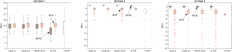
Figure 1: Comparison of the predictive MLS from the simulation study. The three panels provide results for the three cases. Each boxplot is of the 100 values of the MLS from the 100 simulation replicates, where higher values correspond to increased accuracy. In each panel, the first eight boxplots correspond to combinations of the methods BVSC and BVS with the four priors for $g$. The last boxplot (white) corresponds to the mombf/N method. BVSC dominates all other methods in the non-Gaussian cases 2 and 3. This figure appears in color in the electronic version of this article, and any mention of color refers to that version.

Figure 1 gives boxplots of the MLS of the 100 replicates for the three cases in panels (a–c). In each panel, nine methods are considered: the four variants of both BVSC and BVS, and mombf/N. We make three observations. First, the results for BVS are robust with respect to choice of prior for $g$, whereas for BVSC fixing $g=100$ is dominated by the three flexible priors. Second, for the Gaussian data in case 1 BVS is slightly better than BVSC, and mombf/N has the highest variance. Third, BVSC outperforms both BVS and mombf/N substantially in the two non-Gaussian cases 2 and 3, which in case 3 is because the data is generated from a copula model.

4.2.2 Selection Accuracy

The second measure is the precision-recall curve, which is a popular criterion for assessing classification in machine learning. Here, the classification problem is the selection from 20 covariates, using the marginal posteriors $\mbox{Pr}(\gamma_{j}=1|\text{\boldmath$y$})$, $j=1,\ldots,20$, produced by each method. Given a threshold probability value, let TP, FP and FN be true-positive, false-positive and false-negative classification rates, respectively. Then the curve plots Recall=TP/(TP+FN) on the horizontal axis, against Precision=TP/(TP+FP) on the vertical axis, as the threshold probability value varies from 0 to 1. Simultaneously high values of Recall and Precision (i.e. curves that look like a transposed letter ‘L’) indicate accurate classification.

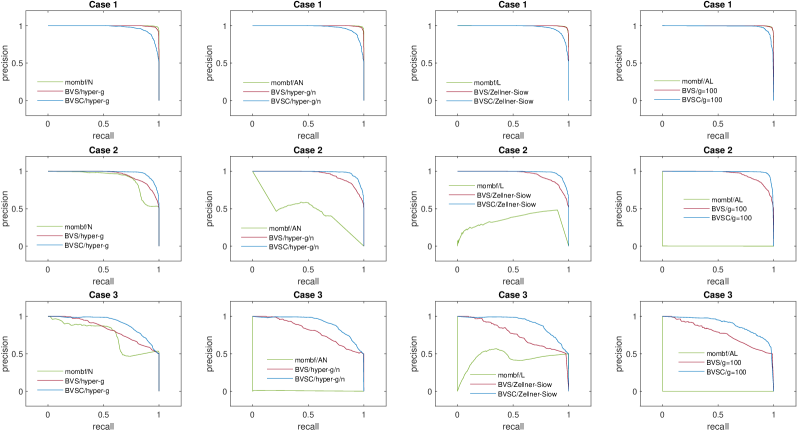
Figure 2: Comparison of the average recall-precision curves from the simulation study for a grid of thresholds in $(0,1)$. The first row (i.e. panels a,b,c,d) show results for case 1, the second row (i.e. panels e,f,g,h) for case 2, and the third row (i.e. panels i,j,k,l) for case 3. Each panel contains curves for the BVSC (blue) and the BVS (red) methods for one specific prior for $g$, along with curves from mombf (green) with one distributional assumption from N (normal), AN (asymmetric normal), L (Laplace) and AL (asymmetric Laplace) in each column. Curves with simultaneously higher recall and precision are more accurate classifiers. This figure appears in color in the electronic version of this article, and any mention of color refers to that version.

Figure 2 plots the average precision-recall curves over the 100 replicates of the simulation. For each case, 12 curves—one for each method and variant—are presented, and we make three observations. First, the asymmetric variants of mombf perform poorly for the non-Gaussian data (cases 2 and 3), despite specifically allowing for this circumstance. Second, the BVSC is much more accurate in cases 2 and 3, where it also outperforms BVS for all variants of priors for $g$. This robustness to distributional form is a result of the flexibility obtained through the non-parametric calibration of the margins. Third, BVSC is less accurate than BVS and mombf only for the Gaussian data generating process (case 1), although the under-performance is minor when compared to the gains obtained in the two non-Gaussian cases.

5 Extension to Spatial BVS for fMRI

An important application of BVS is to construct activation maps in functional magnetic resonance imaging (fMRI) studies. This involves the extension to spatial data located on a regular lattice of ‘voxels’ that partition the brain (Smith et al., 2003; Smith and Fahrmeir, 2007; Goldsmith et al., 2014; Lee et al., 2014). We show how to extend our methodology to this case, and demonstrate that the activation maps can be more accurate when taking into account the non-Gaussianity of the magnetic resonance (MR) signal using our implicit copula-based approach to variable selection. This is consistent with recent work that suggests the MR signal is neither conditionally Gaussian nor homoscedastic (Eklund et al., 2017).

5.1 Marginally calibrated variable selection for fMRI

In fMRI studies, a MR signal $\{Y_{i,t};t=1,\ldots,T\}$ is observed at each voxel $i\in\{1,\ldots,N\}$. This is matched with a series of scalar observations $\{x_{i,t};t=1,\ldots,T\}$ on a transformed stimulus, which is a delayed and continuously modified version of an original stimulus called the ‘hemodynamic response’ that is derived in a pre-processing step outlined in Smith et al. (2003, p.804). The objective in such analyses is to identify at which voxels the MR signal is related to the transformed stimulus (Bezener et al., 2018).

Denote voxel activation by the vector $\text{\boldmath$\gamma$}=(\gamma_{1},\ldots,\gamma_{N})^{\prime}$, such that voxel $i$ is activated by the stimulus if $\gamma_{i}=1$, and inactivate if $\gamma_{i}=0$. Spatial smoothing is essential to obtaining reliable activation maps, which is achieved by using the mass function of an Ising model as a prior

$$p(\text{\boldmath$\gamma$}|\theta)\propto\exp\left(\sum_{i=1}^{N}\delta_{i}\gamma_{i}+\theta\sum_{i\sim j}\omega_{ij}{\cal I}(\gamma_{i}=\gamma_{j})\right)\,.$$

Here, ${\cal I}(A)=1$ if $A$ is true and zero otherwise, and the summation over $i\sim j$ is over all pairwise neighboring elements of $\gamma$ (which are the up to 8 neighbors of each voxel in two dimensions). The weight $\omega_{ij}=1$ for immediately adjacent voxels $i,j$, and $\omega_{ij}=1/\sqrt{2}$ for diagonally adjacent voxels $i,j$, while the parameter $0\leq\theta\leq 0.45$ controls the level of spatial smoothing. The $\delta_{1},\ldots,\delta_{N}$ are coefficients of the external field and determined using a process described in Smith and Fahrmeir (2007, Sec.4.2) that computes each $\delta_{i}$ from the amount of grey matter in voxel $i$ (with more grey matter resulting in a higher value of $\delta_{i}$). This is important because only grey matter can be activated by the stimulus. Alternative binary random fields may also be used as a prior for $\gamma$ in our framework.

To extend our copula model in Section 2.1 to this case, let $\bm{Y}_{i}=(Y_{i,1},\ldots,Y_{i,T})^{\prime}$, $\text{\boldmath$x$}_{i}=(x_{i,1},\ldots,x_{i,T})^{\prime}$, $\text{\boldmath$Y$}=(\text{\boldmath$Y$}_{1}^{\prime},\ldots,\text{\boldmath$Y$}_{N}^{\prime})^{\prime}$ and $\text{\boldmath$x$}=(\text{\boldmath$x$}_{1}^{\prime},\ldots,\text{\boldmath$x$}_{N}^{\prime})^{\prime}$. Also, let $\text{\boldmath$w$}_{t}=(w_{t,1},\ldots,w_{t,m})^{\prime}$ be $m$ basis functions (which we specify later) evaluated at time point $t$ used to capture a localized baseline time trend at each voxel, and $\bm{W}=[\text{\boldmath$w$}_{1}|\ldots|\text{\boldmath$w$}_{T}]^{\prime}$. We assume $Y_{i,t}$ has a voxel-specific marginal distribution function $F_{Y_{i}}(y_{i,t})$ and density $p_{Y_{i}}(y_{i,t})$, and adopt the following copula model for the joint density of $\text{\boldmath$Y$}|\text{\boldmath$x$},\bm{W},\text{\boldmath$\gamma$}$:

$$p(\text{\boldmath$y$}|\text{\boldmath$x$},\bm{W},\text{\boldmath$\gamma$})=\prod_{i=1}^{N}\left(c_{\mbox{\tiny SBVS}}(\text{\boldmath$u$}_{i}|\text{\boldmath$x$}_{i},\bm{W},\gamma_{i})\prod_{t=1}^{T}p_{Y_{i}}(y_{i,t})\right)\,,$$ (12)

where $\text{\boldmath$u$}_{i}=(u_{i,1},\ldots,u_{i,T})^{\prime}$ and $u_{i,t}=F_{Y_{i}}(y_{i,t})$. At (12), the MR signals $\text{\boldmath$Y$}_{1},\ldots,\text{\boldmath$Y$}_{N}$ are independent over voxels when conditioning on $\gamma$, with each vector $\bm{Y}_{i}$ following a copula decomposition as at (1). For the $T$-dimensional copula density $c_{\mbox{\tiny SBVS}}$ we employ an implicit copula derived from a pseudo-regression model, as outlined below in Section 5.2.

Spatial dependence between elements of $\gamma$ is introduced using the Ising model prior, giving posterior mass function $p(\text{\boldmath$\gamma$}|\text{\boldmath$x$},\bm{W},\text{\boldmath$y$})\propto\left(\prod_{i=1}^{N}c_{\mbox{\tiny SBVS}}(\text{\boldmath$u$}_{i}|\text{\boldmath$x$}_{i},\bm{W},\gamma_{i})\right)p(\text{\boldmath$\gamma$}|\theta)$. As in Section 2, variable selection (i.e. the classification of voxels as active or inactive) using this posterior is separated from the task of marginal calibration of the distributions $F_{Y_{1}},\ldots,F_{Y_{N}}$ of the MR signal. We show in our empirical work that this changes the activation maps and improves the quality of fit (measured using mean logarithmic scores) substantially compared to the Gaussian spatial BVS of Smith et al. (2003) and Smith and Fahrmeir (2007).

5.2 Spatial variable selection copula

The implicit copula $c_{\mbox{\tiny SBVS}}$ is of the same form at every voxel, and we derive it here for voxel $i$. It is obtained from the regression $\tilde{Z}_{i,t}=\text{\boldmath$w$}_{t}^{\prime}\text{\boldmath$\alpha$}+x_{i,t}\beta_{\gamma_{i}}+\varepsilon_{i,t}$ for pseudo-response $\tilde{Z}_{i,t}$ at times $t=1,\ldots,T$. Here, $\varepsilon_{i,t}\overset{}{\sim}\operatorname{N}(0,\sigma^{2})$ and $\text{\boldmath$w$}_{t}^{\prime}\text{\boldmath$\alpha$}$ is a time trend with eight low order Fourier terms as basis functions and coefficients $\alpha$, while the transformed stimulus $x_{i,t}$ is a scalar covariate with coefficient $\beta_{\gamma_{i}}$. Variable selection is performed only on $x_{i,t}$, so that $\beta_{\gamma_{i}}=0\mbox{ iff }\gamma_{i}=0$. Smith et al. (2003) and Smith and Fahrmeir (2007) apply regressions of this form directly to the MR signal at each voxel, but here we instead extract its implicit copula for use at (12).

Setting $\widetilde{\text{\boldmath$Z$}}_{i}=(\tilde{Z}_{i,1},\ldots,\tilde{Z}_{i,T})^{\prime}$, the regression can be written as the linear model

$$\widetilde{\text{\boldmath$Z$}}_{i}=\bm{W}\text{\boldmath$\alpha$}+\text{\boldmath$x$}_{i}\beta_{\gamma_{i}}+\text{\boldmath$\varepsilon$}_{i}\,,$$ (13)

with $\text{\boldmath$\varepsilon$}_{i}=(\varepsilon_{i,1},\ldots,\varepsilon_{i,T})^{\prime}$, and $\text{\boldmath$x$}_{i},\bm{W}$ as defined in the previous subsection. Proper priors have to be employed for $\alpha$ and $\beta_{\gamma_{i}}$ to obtain a proper implicit copula. We use the same spike-and-slab prior for $\beta_{\gamma_{i}}$ as previously, so that $\beta_{\gamma_{i}}=0|\gamma_{i}=0$, and $\beta_{\gamma_{i}}|\gamma_{i}=1,g,\sigma^{2}\sim\operatorname{N}\left(0,g\sigma^{2}(\text{\boldmath$x$}_{i}^{\prime}\text{\boldmath$x$}_{i})^{-1}\right)$. We use a $\operatorname{N}(0,\sigma^{2}d\text{\boldmath$I$})$ prior for $\alpha$, with $d$ set to make the prior uninformative, along with the same four priors for $g$ used previously in Section 2.

The same process is used to construct $c_{\mbox{\tiny SBVS}}$ as in Section 2.2, but tailored to account for the time trend in (13). First, the joint distribution $\widetilde{\text{\boldmath$Z$}}_{i}|\text{\boldmath$x$}_{i},\bm{W},\gamma_{i},g,\sigma^{2}\sim N(\bm{0},\mathbf{\Omega})$, with

$$\mathbf{\Omega}=\sigma^{2}\left(\text{\boldmath$I$}+d\bm{W}\bm{W}^{\prime}+\gamma_{i}\left(\frac{g\text{\boldmath$x$}_{i}\text{\boldmath$x$}_{i}^{\prime}}{\text{\boldmath$x$}_{i}^{\prime}\text{\boldmath$x$}_{i}}\right)\right)\,,$$

where $\beta_{\gamma_{i}}$ and $\alpha$ have been integrated out analytically; see Part G.1 of the Web Appendix. Second, the pseudo-response is standardized by the marginal variances of this distribution to give $\bm{Z}_{i}=\sigma^{-1}\bm{S}_{\gamma_{i}}\widetilde{\bm{Z}}_{i}$, with $\bm{S}_{\gamma_{i}}\equiv\operatorname{diag}(s_{1}(\gamma_{i}),\ldots,s_{T}(\gamma_{i}))$ and $s_{t}(\gamma_{i})=\left(1+d\text{\boldmath$w$}_{t}^{\prime}\text{\boldmath$w$}_{t}+\gamma_{i}\left(\frac{gx_{i,t}^{2}}{\text{\boldmath$x$}_{i}^{\prime}\text{\boldmath$x$}_{i}}\right)\right)^{-\frac{1}{2}}$. Thus, $\text{\boldmath$Z$}_{i}|\text{\boldmath$x$}_{i},\bm{W},\gamma_{i},g,\sigma^{2}\sim\operatorname{N}\left(\bm{0},\bm{R}(\text{\boldmath$x$}_{i},\bm{W},\gamma_{i},g)\right)$, where

$$\bm{R}(\text{\boldmath$x$}_{i},\bm{W},\gamma_{i},g)=\bm{S}_{\gamma_{i}}\left(\text{\boldmath$I$}+d\bm{W}\bm{W}^{\prime}+\gamma_{i}\frac{g\text{\boldmath$x$}_{i}\text{\boldmath$x$}_{i}^{\prime}}{\text{\boldmath$x$}_{i}^{\prime}\text{\boldmath$x$}_{i}}\right)\bm{S}_{\gamma_{i}}\,,$$ (14)

is a correlation matrix, and the implicit copula of both $\widetilde{\bm{Z}}_{i}$ and $\bm{Z}_{i}$ (conditional on $\text{\boldmath$x$}_{i},\bm{W},\gamma_{i},g,\sigma^{2}$) is a Gaussian copula with parameter matrix $\bm{R}$ defined at (14). Finally, we obtain $c_{\mbox{\tiny SBVS}}$ by mixing over the prior for $g$, which we formalize in the following definition.

Definition 2

Let $c_{\mbox{\tiny{Ga}}}$ be the Gaussian copula density with the correlation matrix $\bm{R}$ defined at (14). If $p(g)$ is a proper prior density for $g>0$, then we call

$$c_{\mbox{\tiny SBVS}}(\bm{u}|\text{\boldmath$x$}_{i},\bm{W},\gamma_{i})=\int c_{\mbox{\tiny{Ga}}}(\bm{u};\bm{R}(\text{\boldmath$x$}_{i},\bm{W},\gamma_{i},g))p(g)\mathrm{d}g\,.$$

the density function of a spatial variable selection copula.

As in Section 2, $\sigma^{2}$ does not feature in the expression for $\bm{R}$ nor the copula density. We use this copula at (12), where the transformed stimulus values $\text{\boldmath$x$}_{i}$ and activation indicator $\gamma_{i}$ vary over voxels, whereas the matrix of linear time trend basis terms $\bm{W}$ does not.

5.3 Estimation and inference

Parameter estimation and posterior inference is obtained using an adaptation of the sampler in Section 3.1 that is presented in detail in Parts G.2 and G.3 of the Web Appendix. It is a single-site sampler in the elements of $\text{\boldmath$\gamma$}=(\gamma_{1},\ldots,\gamma_{N})^{\prime}$, which is more computationally efficient than multi-site samplers (e.g. Nott and Green (2004)) because key quantities can be pre-computed just once. This is important when undertaking variable selection in fMRI studies due to the large number of voxels $N$. The parameter $g$ is generated using a Metropolis-Hastings (MH) step with a Gaussian approximation as a proposal. This has an acceptance rate of over 80%, and replaces the HMC step in Section 3. The spatial smoothing parameter $\theta$ is generated using an adaptive random walk MH step.

Accurate Monte Carlo mixture estimates of the marginal posteriors $\mbox{Pr}(\gamma_{i}=1|\text{\boldmath$x$},\bm{W},\text{\boldmath$y$})$ can be readily computed from the conditional posteriors of the single site sampler. Plots of these are Bayesian estimates of the activation maps. An accompanying output is the map of posterior means of the amplitudes $\beta_{\gamma_{1}},\ldots,\beta_{\gamma_{N}}$, for which an efficient mixture estimate can also be constructed, as outlined in Part G.4 of the Web Appendix.

Table 2: Results from applying both the copula (SBVSC) and Gaussian (SBVS) spatial Bayesian variable selection methods to the fMRI data. The four different priors are used for $g$, giving a total of eight methods. The top rows report the mean logarithmic scores (MLS) of the MR signal (multiplied by 100 for presentation), broken down voxels classified as active, inactive and overall. Higher MLS values indicate greater accuracy. The bottom rows report the posterior mean and standard deviation of the number of active voxels $q_{\gamma}=\sum_{j=1}^{N}\gamma_{j}$.

Prior	hyper-g		hyper-g/$n$		Zellner-Siow		$g=100$
Model	SBVSC	SBVS	SBVSC	SBVS	SBVSC	SBVS	SBVSC	SBVS
Active	-411.65	-450.72	-411.65	-450.72	-411.65	-450.72	-418.37	-451.08
Inactive	-408.12	-416.48	-408.12	-416.48	-408.12	-416.48	-408.32	-416.53
Overall	-408.18	-416.92	-408.18	-416.92	-408.17	-416.92	-408.42	-416.96
$\text{$\mathds{E}$}(q_{\gamma}|\text{\boldmath$y$})$	110.8	162.0	110.8	162.0	110.8	162.0	72.1	119.5
$\mbox{Std}(q_{\gamma}|\text{\boldmath$y$})$	3.1	13.9	3.1	13.9	3.1	13.9	2.3	8.6

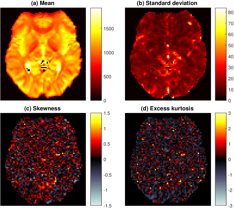
Figure 3: Sample moments of the MR signal at each voxel in the fMRI example. The four panels plot the (a) mean, (b) standard deviation, (c) Pearson skew and (d) excess kurtosis values for each voxel. Computation of the global Moran’s I spatial correlation coefficients indicates that there is strong spatial correlation in all four sample moments. This figure appears in color in the electronic version of this article, and any mention of color refers to that version.

5.4 Empirical results

To illustrate, we construct activation maps for slice 10 of individual B in Smith et al. (2003). This data includes an MR signal observed at $T=63$ time points and $N=72\times 86$ voxels from a simple visual experiment. Activation is therefore largely in the visual cortex. Figure 3 plots the first four sample moments of the MR time series at each voxel, indicating a considerable deviation from normality at many voxels. This is not captured in the Gaussian spatial BVS model (labelled ‘SBVS’ here). In contrast, our spatial BVS copula model (labelled ‘SBVSC’ here) does so using non-parametric estimators for $F_{Y_{1}},\ldots,F_{Y_{N}}$.

We estimate the SBVSC parameters for all four priors for $g$. For comparison, we also estimate the SBVS model of Smith et al. (2003) using the same priors for $g,\theta,\text{\boldmath$\gamma$}$ as in the copula model. To compare the two sets of results, Table 2 reports the mean (in-sample) logarithmic scores for both the SBVS and SBVSC models, and for each prior of $g$. To compute these we evaluate the mean in-sample logarithmic scores at each voxel $i$ as $1/T\sum_{t=1}^{T}\log(\hat{p}(y_{i,t}|\text{\boldmath$x$}))$, and then average the results across active, inactive and all voxels. The predictive densities are computed using a minor adjustment to (11) to account for the time trend terms; see Part G.5 of the Web Appendix. We make three observations. First, in all cases the SBVSC scores are higher than those for SBVS. The relative improvement is 9.5% for voxels classified as active by SBVSC, and 2% across all voxels. Second, for SBVSC setting $g=100$ degrades the results, although there is no difference between the other three priors for $g$. Third, the expected number of active voxels is lower for SBVSC, producing a sparser image than SBVS.

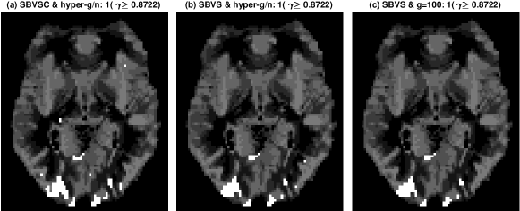
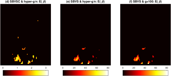
Figure 4: Posterior activation and amplitude maps for the fMRI data from three different estimators. The first row shows the activation maps (where white voxels are those classified as active), and the second shows the mean activation amplitudes. The three different estimators are: (a,d) SBVSC with hyper-g/n prior; (b,e) SBVS with hyper-g/n prior; and, (c,f) SBVS with $g=100$. This figure appears in color in the electronic version of this article, and any mention of color refers to that version.

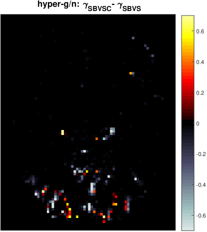
Figure 5: Difference between the activation probabilities of the copula (SBVSC) and Gaussian (SBVS) spatial Bayesian variable selection models for the fMRI data. The difference is SBVSC minus SBVS, and both models employ the same Ising prior for $\gamma$ and hyper-g/n prior for $g$. This figure appears in color in the electronic version of this article, and any mention of color refers to that version.

Based on these observations, Figure 4 compares activation and amplitude maps for three cases: panels (a,d) SBVSC with hyper-g/n prior; (b,e) SBVS with hyper-g/n prior; and (c,f) SBVS with $g=100$. The latter case is included because it is the benchmark model suggested by Smith and Fahrmeir (2007). The activation maps in the first row are obtained by defining a voxel as active if and only if $\mbox{Pr}(\gamma_{i}=1|\text{\boldmath$x$},\bm{W},\text{\boldmath$y$})\geq 0.8722$. The justification for this threshold value is that $-2\log((1-\mbox{Pr}(\gamma_{i}=1|\text{\boldmath$x$},\bm{W},\text{\boldmath$y$}))/\mbox{Pr}(\gamma_{i}=1|\text{\boldmath$x$},\bm{W},\text{\boldmath$y$})$ is approximately $\chi^{2}(1)$ distributed and the threshold corresponds to a p-value of 0.05. The maps for the two SBVS models are close to identical, but differ from those for the SBVSC model, with the latter allowing for sharper edges in the amplitude maps. To further highlight this difference, Figure 5 plots the difference in the activation probabilities between the copula and Gaussian models. These differ between -0.6 and 0.6, so that allowing for more accurate marginal calibration of the MR signal not only increases the logarithmic scores, but affects activation maps, which are the primary output of fMRI processing.

Both samplers were implemented efficiently in MATLAB. The time to undertake 1000 sweeps was approximately 10 mins (SBVS) and 11 mins (SBVSC) when $g$ is generated, and 2 mins (SBVS) and 2.3 mins (SBVSC) when $g$ is fixed. Thus, marginally-calibrated spatial BVS is only slightly slower than Gaussian spatial BVS, and can be made even faster using a lower level language. Typically, only a few thousand sweeps are needed to obtain highly accurate maps, because the Markov chain converges quickly and mixture estimators are used. While not undertaken here, the speed of the approach allows application to multiple slices using the 3D Markov random field prior for $\gamma$ in Smith and Fahrmeir (2007).

6 Discussion

This paper proposes a new tractable and general approach to undertake BVS for non-Gaussian data. It uses a copula decomposition that allows the marginal distribution of the dependent variable to be calibrated accurately using nonparametric estimation. However, we note that this does not imply the other forms of calibration or dispersion listed by Gneiting et al. (2013). In addition, a referee pointed out that the assumption at (1) that $F_{Y}$ is independent of $\bm{X}$ limits the range of distributions for $\bm{Y}|\bm{X}$ that can be represented. However, this assumption separates the variable selection problem from that of marginal calibration, which is a major advantage of our proposed approach.

The key ingredient of our methodology is a family of implicit copulas that are constructed from a regression model for a Gaussian pseudo-response with spike-and-slab priors. These mix over the different priors in Liang et al. (2008) for the scaling factor of the g-prior, producing the copula family at Defn. 1 which is a continuous mixture of Gaussian copulas. We apply our approach to an example with 6192 spatially correlated indicators, and to second example with $p=252$ correlated covariates in Part F of the Web Appendix. The empirical work demonstrates that mixing over the priors for $g$ (particularly the hyper-g prior) results in much more accurate covariate selection and predictive densities of the dependent variable, compared to fixing $g$. This is in contrast to Gaussian Bayesian variable selection, where in some examples fixed $g$ (such as $g=100$ or $g=n$) can provide good results (Smith and Kohn, 1996). Moreover, in the second example we also find that integrating out uncertainty in $F_{Y}$ as in Grazian and Liseo (2017) does not meaningfully effect covariate selection or prediction. The method is scalable to higher dimensions because estimation by stochastic search over $\gamma$ is fast when exploiting the matrix identities in the Web Appendix. The extension of the method to spatial BVS for fMRI—an important contemporary application (Lee et al., 2014; Bezener et al., 2018)—highlights its tractability.

While the use of copulas to capture dependence between multiple observations on one or more variables is rare, there are some recent examples. In regression these include implicit copulas constructed from Gaussian processes (Wilson and Ghahramani, 2010; Wauthier and Jordan, 2010) or regularized basis functions (Klein and Smith, 2019). In time series analysis, copulas have been used to capture serial dependence in univariate and multivariate data; for example, see Smith (2015) and Shi and Yang (2018). These studies all exploit a copula decomposition to allow for non-Gaussian margins. However, ours is the first study to employ our proposed copula formulation to undertake variable selection.

We finish by making some suggestions for future work. A potential extension is to multivariate regression (i.e. with multiple dependent variables), generalizing the approaches of Brown et al. (1998), Smith and Kohn (2000) and others. To do so requires the specification of an implicit copula analogous to that in Defn. 1. It would also be interesting to explore the relationship between properties of $c_{\mbox{\tiny BVS}}$, such as the dependence metrics in Part C of the Web Appendix, and covariate selection accuracy. Last, the implicit copula can be extended to other Bayesian models for fMRI data that are based on alternative specifications of (13), such as that in Lee et al. (2014). This would lead to other copula processes on the covariate space with strong potential to further improve voxel classification accuracy.

Data Availability

The data that support the findings in this paper are available in the Supporting Information.

Supporting Information

Online Appendices, Tables, and Figures referenced in Sections 1 through 5 are available with this paper at the Biometrics website on Wiley Online Library. MATLAB code to reproduce the results for the fMRI data in Section 5 is also available at the same website.

References

- (1)
- Bezener et al. (2018) Bezener, M., Hughes, J. and Jones, G. (2018). Bayesian spatiotemporal modeling using hierarchical spatial priors, with applications to functional magnetic resonance imaging (with discussion), Bayesian Analysis 13(4): 1261–1313.
- Bottolo and Richardson (2010) Bottolo, L. and Richardson, S. (2010). Evolutionary stochastic search for Bayesian model exploration, Bayesian Analysis 5(3): 583–618.
- Brown et al. (1998) Brown, P. J., Vannucci, M. and Fearn, T. (1998). Multivariate Bayesian variable selection and prediction, Journal of the Royal Statistical Society: Series B 60(3): 627–641.
- Chung and Dunson (2009) Chung, Y. and Dunson, D. (2009). Nonparametric Bayes conditional distribution modeling with variable selection, Journal of the American Statistical Association 104: 1646–1660.
- Eklund et al. (2017) Eklund, A., Lindquist, M. A. and Villani, M. (2017). A Bayesian heteroscedastic GLM with application to fMRI data with motion spikes, Neuroimage 155: 354–369.
- George and McCulloch (1993) George, E. and McCulloch, R. (1993). Variable selection via Gibbs sampling, Journal of the American Statistical Association 88: 881–889.
- George and McCulloch (1997) George, E. and McCulloch, R. (1997). Approaches to Bayesian variable selection, Statistica Sinica 7: 339–374.
- Gneiting et al. (2007) Gneiting, T., Balabdaoui, F. and Raftery, A. E. (2007). Probabilistic forecasts, calibration and sharpness, Journal of the Royal Statistical Society: Series B 69(2): 243–268.
- Gneiting et al. (2013) Gneiting, T., Ranjan, R. et al. (2013). Combining predictive distributions, Electronic Journal of Statistics 7: 1747–1782.
- Goldsmith et al. (2014) Goldsmith, J., Huang, L. and Crainiceanu, C. M. (2014). Smooth scalar-on-image regression via spatial Bayesian variable selection, Journal of Computational and Graphical Statistics 23(1): 46–64.
- Gottardo and Raftery (2009) Gottardo, R. and Raftery, A. (2009). Bayesian robust transformation and variable selection: A unified approach, Canadian Journal of Statistics 37(3): 361–380.
- Grazian and Liseo (2017) Grazian, C. and Liseo, B. (2017). Approximate Bayesian inference in semiparametric copula models, Bayesian Analysis 12(4): 991–1016.
- Griffin et al. (2017) Griffin, J., Latuszynski, K. and Steel, M. (2017). In search of lost (mixing) time: Adaptive Markov chain Monte Carlo schemes for Bayesian variable selection with very large , arXiv preprint, 1708.05678 .
- Hoffman and Gelman (2014) Hoffman, M. D. and Gelman, A. (2014). The No-U-Turn sampler: Adaptively setting path lengths in Hamiltonian Monte Carlo, Journal of Machine Learning Research 15: 1351–1381.
- Joe (2005) Joe, H. (2005). Asymptotic efficiency of the two-stage estimation method for copula-based models, Journal of Multivariate Analysis 94(2): 401–419.
- Johnson and Rossell (2012) Johnson, V. E. and Rossell, D. (2012). Bayesian model selection in high-dimensional settings, Journal of the American Statistical Association 107(498): 649–660.
- Klein and Smith (2019) Klein, N. and Smith, M. S. (2019). Implicit copulas from Bayesian regularized regression smoothers, Bayesian Analysis 14(4): 1143–1171.
- Kraus and Czado (2017) Kraus, D. and Czado, C. (2017). D-vine copula based quantile regression, Computational Statistics & Data Analysis 110: 1–18.
- Kundu and Dunson (2014) Kundu, S. and Dunson, D. B. (2014). Bayes variable selection in semiparametric linear models, Journal of the American Statistical Association 109(505): 437–447.
- Lee et al. (2014) Lee, K.-J., Jones, G. L., Caffo, B. S. and Bassett, S. S. (2014). Spatial Bayesian variable selection models on functional magnetic resonance imaging time-series data, Bayesian Analysis 9(3): 699.
- Li and Zhang (2010) Li, F. and Zhang, N. R. (2010). Bayesian variable selection in structured high-dimensional covariate spaces with applications in genomics, Journal of the American Statistical Association 105(491): 1202–1214.
- Liang et al. (2008) Liang, F., Paulo, R., Molina, G., Clyde, M. A. and Berger, J. O. (2008). Mixtures of g priors for Bayesian variable selection, Journal of the American Statistical Association 103(481): 410–423.
- Neal (2011) Neal, R. M. (2011). MCMC using Hamiltonian dynamics, in S. Brooks, A. Gelman, G. Jones and X.-L. Meng (eds), Handbook of Markov Chain Monte Carlo, CRC Press, pp. 113–162.
- Nelsen (2006) Nelsen, R. (2006). An Introduction to Copulas, 2nd edn, Springer.
- Nott and Green (2004) Nott, D. J. and Green, P. J. (2004). Bayesian variable selection and the Swendsen-Wang algorithm, Journal of Computational and Graphical Statistics 13(1): 141–157.
- O’Hara and Sillanpää (2009) O’Hara, R. and Sillanpää, M. (2009). A review of Bayesian variable selection methods: What, How, and Which, Bayesian Analysis 4: 85–118.
- Rossell and Rubio (2018) Rossell, D. and Rubio, F. J. (2018). Tractable Bayesian variable selection: beyond normality, Journal of the American Statistical Association 113(524): 1742–1758.
- Sharma and Das (2018) Sharma, R. and Das, S. (2018). Regularization and variable selection with copula prior, arXiv:1709.05514v2 .
- Shi and Yang (2018) Shi, P. and Yang, L. (2018). Pair copula constructions for insurance experience rating, Journal of the American Statistical Association 113(521): 122–133.
- Shimazaki and Shinomoto (2010) Shimazaki, H. and Shinomoto, S. (2010). Kernel bandwidth optimization in spike rate estimation, Journal of Computational Neuroscience 29(1-2): 171–182.
- Smith et al. (2003) Smith, M., Pütz, B., Auer, D. and Fahrmeir, L. (2003). Assessing brain activity through spatial Bayesian variable selection, NeuroImage 20(2): 802–815.
- Smith (2015) Smith, M. S. (2015). Copula modelling of dependence in multivariate time series, International Journal of Forecasting 31: 815–833.
- Smith and Fahrmeir (2007) Smith, M. S. and Fahrmeir, L. (2007). Spatial Bayesian variable selection with application to functional magnetic resonance imaging, Journal of the American Statistical Association 102(478): 417–431.
- Smith and Kohn (1996) Smith, M. S. and Kohn, R. (1996). Nonparametric regression using Bayesian variable selection, Journal of Econometrics 75(2): 317–343.
- Smith and Kohn (2000) Smith, M. S. and Kohn, R. (2000). Nonparametric seemingly unrelated regression, Journal of Econometrics 98: 257–281.
- Song (2000) Song, P. (2000). Multivariate dispersion models generated from Gaussian copula, Scandinavian Journal of Statistics 27(2): 305–320.
- Wauthier and Jordan (2010) Wauthier, F. L. and Jordan, M. I. (2010). Heavy-tailed process priors for selective shrinkage, Advances in Neural Information Processing Systems, pp. 2406–2414.
- Wilson and Ghahramani (2010) Wilson, A. G. and Ghahramani, Z. (2010). Copula processes, Advances in Neural Information Processing Systems, pp. 2460–2468.
- Yu et al. (2013) Yu, K., Chen, C., Reed, C. and Dunson, D. (2013). Bayesian variable selection in quantile regression, Statistics and its interface 6: 261–274.