Two-block vs. Multi-block ADMM:
An empirical evaluation of convergence

Abstract

Alternating Direction Method of Multipliers (ADMM) has become a widely used optimization method for convex problems, particularly in the context of data mining in which large optimization problems are often encountered. ADMM has several desirable properties, including the ability to decompose large problems into smaller tractable sub-problems and ease of parallelization, that are essential in these scenarios. The most common form of ADMM is the two-block, in which two sets of primal variables are updated alternatingly. Recent years have seen advances in multi-block ADMM, which update more than two blocks of primal variables sequentially. In this paper, we study the empirical question: Is two-block ADMM always comparable with sequential multi-block ADMM solving an equivalent problem? In the context of optimization problems arising in multi-task learning, through a comprehensive set of experiments we surprisingly show that multi-block ADMM consistently outperformed two-block ADMM on optimization performance, and as a consequence on prediction performance, across all datasets and for the entire range of dual step sizes. Our results have an important practical implication: rather than simply using the popular two-block ADMM, one may considerably benefit from experimenting with multi-block ADMM applied to an equivalent problem.

Keywords Alternating Direction Method of Multipliers  $\cdot$ Two-block ADMM  $\cdot$ Multi-block ADMM  $\cdot$ Convergence Analysis  $\cdot$ Nonconvex optimization  $\cdot$ Multitask Learning

1 Introduction

The past decade has seen wide ranging applications of the alternating direction method of multipliers (ADMM) for different learning problems [1, 2, 3, 4]. The success of ADMM in the context of data mining can be attributed to its ability to decouple large problems into smaller tractable sub-problems, simplicity of the updates (sometimes in closed form) for these individual sub-problems, ease of parallelization, among others. ADMM has also been widely applied to unconstrained non-smooth problems, such as the lasso and fused lasso, by introducing additional variables (lifting) thereby decoupling smooth and non-smooth terms [5, 4].

The most popular version of ADMM is the two-block ADMM which considers the following problem:

$$\min_{x,z}~{}f(x)+g(z)\quad\text{s.t.}\quad Ax+Bz=c~{},$$ (1)

where $x\in\mathbb{R}^{n},z\in\mathbb{R}^{m},A\in\mathbb{R}^{d\times n},B\in\mathbb{R}^{d\times m},c\in\mathbb{R}^{d}$ [6, 7, 8, 9]. The formulation is called two-block because of the two sets of variables $(x,z)$ which are updated alternatingly in the primal updates of ADMM. Recent years have seen the use of multi-block ADMM in some settings [6, 10, 11, 12], which considers more than two sets of variables which are sequentially updated in the primal. The literature has also looked at potential challenges in doing naive multi-block ADMM, and several approaches to doing it with theoretical guarantees of convergence have been developed [13, 14, 12].

Two-block ADMM is by far the most widely used variant of ADMM. In practice, often two-block ADMM is used without much thought regarding alternative multi-block ADMM options. For convex problems, they are supposed to give the same solution after all, with suitable choices of (dual) step sizes. Typically, a multi-block problem can be solved as a two-block problem with suitable variable and constraint grouping, and similarly two-block problems can be converted into multi-block by suitable lifting [6, 10, 15]. Our work is motivated by a desire to understand why two-block ADMM is preferred. A part of the reason may be the seemingly negative theoretical results associated with convergence of multi-block ADMM [11]. In many cases, such negative theoretical results focused on a specific problem or operating regimes where multi-block ADMM diverges. In practice, most optimization methods have such weak spots in terms of struggling in a type of problem or operating regime, e.g., the simplex algorithm for linear programs [16], stochastic gradient descent (SGD) for deep networks [17], etc. In many cases, such algorithms are empirically successful and it takes a while to improve our theoretical understanding of its behavior, e.g., smoothed analysis of the simplex algorithm [18], convergence of SGD on non-convex problems [19, 20, 21, 22], etc. Such perspective motivates our empirical work on two-block vs. multi-block ADMM comparisons.

In particular, in this paper we study the empirical question: Is two-block ADMM always comparable with multi-block ADMM solving an equivalent problem? For both two-block and multi-block ADMM, we consider linearized ADMM [2] which has considerably computational benefits and keep the (dual) step size as the only hyper-parameter. Also, for multi-block ADMM, we use the direct extension from two-block ADMM which sequentially updates the primal variables [1]. We perform experiments using optimization problems arising in multi-task learning (MTL), with application focus on modeling Alzheimer’s disease progression, Parkinson’s disease assessment, and air quality prediction. For each problem, we conduct a direct comparison between two-block and multi-block ADMM by varying one hyper-parameter—the dual step-size in ADMM (see Section 4 and 5 for details)– up to 5 orders of magnitude, running each method for 1,000 iterations, and for 10,000 iterations in some cases, and repeating each experiment 10 times to account for any inherent variability. The approaches are evaluated based on different evaluation measures including primal residual convergence and prediction performance on validation set (see Section 5).

Our results are surprising: multi-block ADMM empirically outperformed two-block ADMM on optimization performance, and as a consequence on prediction performance, across all datasets and for the entire range of dual step sizes. For optimization performance, multi-block ADMM achieves primal residuals which are a few orders of magnitude smaller than that achieved by two-block ADMM, implying a better convergence to the feasible set. Note that primal iterates in any form of ADMM are always outside the feasible set, so having a really small primal residual is important to ensure good convergence, and multi-block ADMM illustrates desirable performance here. Multi-block ADMM also achieves smaller primal objective, which is especially interesting when primal residuals are small. Finally, the models estimated using multi-block ADMM consistently outperforms the corresponding two-block versions on prediction performance evaluated on validation sets.

The take-away from the results reported is the following: if a situation calls for ADMM based optimization, rather than using the popular two-block version by default, one needs to try out equivalent multi-block versions and compare their performance. The results reported do not imply that multi-block ADMM will outperform two-block ADMM on every problem, but that one needs to at least consider multi-block as a serious alternative rather than defaulting to the two-block version due to its popularity. Thus, the contribution of the work is empirical, hoping to change the way our community uses ADMM based algorithms.

The rest of the paper is organized as follows. We review related work in Section 2. We present the MTL model in Section 3 and discuss two-block and multi-block ADMM for learning the model in Section 4. We present detailed results comparing the algorithms in Section 5 and conclude in Section 6.

2 Related Work

The success of ADMM with two blocks has encouraged the natural extension of ADMM to solve problems with multiple blocks [15, 10, 23, 24, 6]. Theoretical results [11] have shown that without additional conditions, the direct extension of ADMM with more than two blocks generally fails to converge. But for certain specific classes of problems and/or conditions, researchers have been able to show convergence guarantees for variants of multi-block ADMM. The existing variants of multi-block ADMM can be mainly grouped into two categories: Gauss-Seidel ADMM and Jacobi ADMM.

The Gauss-Seidel ADMM (GSADMM) [24, 23] seeks to solve the primal updates in a cyclic block coordinate fashion. In [7], a back substitution step was added, which facilitated the convergence proof for ADMM with multiple blocks. In [23], a block successive upper bound minimization method of multipliers (BSUMM) is proposed to solve the problem. In [25], the authors proved that multi-block ADMM can achieve $\epsilon$-optimal solutions within $O(1/\epsilon^{2})$ iterations by solving a modified version of the original problem, and whitin $O(1/\epsilon)$ iterations when applied to certain sharing problems conditioned on properties of the augmented Lagrangian function. Theoretical convergence of some of these methods need fairly strict conditions, e.g., certain local error bounds need to hold and/or the step size needs to be sufficiently small or decreasing.

Another broad approach to multi-block ADMM is Jacobi ADMM [15, 6, 26], which solves the problem in a parallel block coordinate fashion. In [15, 26], the problem is solved by using two-block ADMM with splitting variables (sADMM). [6] considers a proximal Jacobian ADMM (PJADMM) by adding proximal terms. A randomized block coordinate variant of ADMM named RBSUMM was proposed in [23]. Recently, [27] demonstrated that ADMM is convergent regardless of the number of variable blocks for certain nonconvex consensus and sharing problems.

Although general theoretical aspects of multi-block ADMM are still not well understood, it has been observed that modified versions of ADMM, including the two-block instance, though with convergence guarantee, often perform slower than the multi-block ADMM with no convergent guarantee [25]. It is thus of great interest to further study the practical aspects of convergence of multi-block ADMM. Aiming to address the lack of numerical experiments, we systematically investigate the convergence and performance of two-block and multi-block ADMM in the context of multitask learning, which has significantly benefited from advances in ADMM-type of methods.

3 Temporally Smooth Multi-task Learning (TS-MTL)

Consider a multi-task learning problem over $T$ tasks, where each task corresponds to a time point $t=1,\ldots,T$. For each time point $t$, we consider a regression task based on data $(\mathbf{y}_{t},X_{t})$, where $X_{t}\in\mathbb{R}^{n\times p}$ denotes the matrix of covariates, $p$ is the number of covariates and $n$ is the number of samples, shared across all the tasks, and $\mathbf{y}_{t}\in\mathbb{R}^{n}$ is the matrix of responses. Let $\Theta\in\mathbb{R}^{p\times T}$ denote the regression parameter matrix over all tasks, so that column $\boldsymbol{\theta}_{t}\in\mathbb{R}^{p}$ corresponds to the parameters for the task in time step $t$. This multitask learning formulation is based on our recent work [28].

We pose the multi-task learning problem for $\Theta$ such that two goals are accomplished: each $\theta_{t}$ accomplishes low regression error for each task $t$, and “nearby” $\theta_{t}$ are coupled to be similar, since the “nearby” tasks are temporarily related. The notion of “nearby” needs to be suitably defined. In this paper, we adopt an approach inspired by non-parametric regression [29], which has been recently shown to be effective for TS-MTL problems. In particular, we model a local approximation to $\theta_{t}$ in terms of the other $\theta_{\ell},\ell\neq t$ as

$$\hat{\boldsymbol{\theta}}_{t}=\sum_{\begin{subarray}{c}\ell=1\\ \ell\neq t\end{subarray}}^{T}w_{\ell,t}\boldsymbol{\theta}_{\ell},~{}\forall t,w_{\ell,t}=\frac{\exp\left(-\frac{(\ell-t)^{2}}{\sigma^{2}}\right)}{\sum_{\begin{subarray}{c}\ell^{\prime}=1\\ \ell^{\prime}\neq t\end{subarray}}^{T}\exp\left(-\frac{(\ell^{\prime}-t)^{2}}{\sigma^{2}}\right)}~{},\forall\ell\neq t,$$

where $\sigma\geq 0$ is a constant bandwidth parameter. Based on such an approximation, our TS-MTL formulation focus on encouraging sparsity of the residual

$$\boldsymbol{\theta}_{t}-\hat{\boldsymbol{\theta}}_{t}=\boldsymbol{\theta}_{t}-\sum_{\begin{subarray}{c}\ell=1\\ \ell\neq t\end{subarray}}^{T}w_{\ell,t}\boldsymbol{\theta}_{\ell}~{},~{}\forall t~{}.$$ (2)

The TS-MTL problem can now be posed as the following unconstrained problem:

$$\begin{split}\underset{\Theta,\Gamma}{\text{min}}~{}\sum_{t=1}^{T}&\|\mathbf{y}_{t}-X_{t}\boldsymbol{\theta}_{t}\|^{2}+R_{\lambda_{2}}^{\lambda_{1}}(\Theta)+\lambda_{3}\sum_{t=1}^{T}\|\boldsymbol{\theta}_{t}-\sum_{\begin{subarray}{c}\ell=1\\ \ell\neq t\end{subarray}}^{T}w_{\ell,t}\boldsymbol{\theta}_{\ell}\|_{1}~{},\end{split}$$ (3)

where $R_{\lambda_{2}}^{\lambda_{1}}(\Theta)$ is the combination of lasso and group lasso penalties, also known as the sparse group Lasso penalty, which allows simultaneous joint feature selection for all tasks and selection of a specific set of features for each task [30]. In particular,

$$R_{\lambda_{2}}^{\lambda_{1}}(\Theta)=\lambda_{1}\|\Theta\|_{1}+\lambda_{2}\|\Theta\|_{2,1}~{},$$ (4)

where $\|\Theta\|_{1}$ is the Lasso penalty and $\|\Theta\|_{2,1}=\sum_{j=1}^{p}\|\boldsymbol{\theta}_{j}\|,\boldsymbol{\theta}_{j}\in\mathbb{R}^{T}$ is the group Lasso penalty considering groups across time for each feature $j$, encouraging the regression models at different time points to share a common set of features. In the formulation, $\lambda_{1},\lambda_{2},\lambda_{3}>0$ are the regularization parameters which are fixed, and will be chosen using cross validation.

4 ADMM for Learning TS-MTL Models

The unconstrained optimization problem in (3) can be difficult to optimize directly due to the non-smooth terms. In this section, we consider two formulations, respectively solved as a two-block and multi-block ADMM, which introduce additional variables and associated linear constraints. While the use of two-block or multi-block ADMM for solving the problem is not especially novel, through extensive experiments in Section 5 we will show that the two formulations and associated ADMM algorithms behave surprisingly differently in practice.

We start by noting that the optimization problem in (3) can be formulated as the following linearly constrained optimization problem:

$$\underset{\Theta,\Gamma,Q,\Pi}{\text{min}} \sum_{t=1}^{T}\frac{1}{2}\|\mathbf{y}_{t}-X_{t}\boldsymbol{\theta}_{t}\|^{2}+R_{\lambda_{2}}^{\lambda_{1}}(Q)+\lambda_{3}\|\Pi\|_{1}$$ (5)

subject to $$\Theta-Q=0,~{}\mathbf{q}_{t}-\sum_{\begin{subarray}{c}\ell=1\\ \ell\neq t\end{subarray}}^{T}w_{|t-\ell|}\mathbf{q}_{\ell}-\boldsymbol{\gamma}_{t}=0~{}\forall t,~{}\Gamma-\Pi=0~{}.$$

Note that there are four variables $\Theta,\Gamma,Q,\Pi\in\mathbb{R}^{p\times T}$ in the formulation. The problem can also be formulated as

$$\underset{\Theta,\Gamma,Q,\Pi}{\text{min}} ~{}~{}\sum_{t=1}^{T}\frac{1}{2}\|\mathbf{y}_{t}-X_{t}\boldsymbol{\theta}_{t}\|^{2}+R_{\lambda_{2}}^{\lambda_{1}}(Q)+\lambda_{3}\|\Pi\|_{1}$$ (6)

subject to $$\Theta-Q=0,~{}\boldsymbol{\theta}_{t}-\sum_{\begin{subarray}{c}\ell=1\\ \ell\neq t\end{subarray}}^{T}w_{|t-\ell|}\boldsymbol{\theta}_{\ell}-\boldsymbol{\gamma}_{t}=0~{}\forall t,~{}\Gamma-\Pi=0~{}.$$

The only difference between (5) and (6) is the form of the constraint associated with temporal smoothness residuals:

$$\boldsymbol{\gamma}_{t}=\mathbf{q}_{t}-\sum_{\begin{subarray}{c}\ell=1\\ \ell\neq t\end{subarray}}^{T}w_{|t-\ell|}\mathbf{q}_{\ell}~{}\quad\text{vs.}\quad\boldsymbol{\gamma}_{t}=\boldsymbol{\theta}_{t}-\sum_{\begin{subarray}{c}\ell=1\\ \ell\neq t\end{subarray}}^{T}w_{|t-\ell|}\boldsymbol{\theta}_{\ell}~{},$$ (7)

but the constraints are equivalent since $\Theta=Q$.

4.1 Linearized Two-Block ADMM

The augmented Lagrangian $L_{\rho}=L_{\rho}(\Theta,\Gamma,Q,\Pi,S,U,V)$ for (5) is given by:

$$L_{\rho}= \sum_{t=1}^{T}\frac{1}{2}\|\mathbf{y}_{t}-X_{t}\boldsymbol{\theta}_{t}\|^{2}+R_{\lambda_{2}}^{\lambda_{1}}(Q)+\lambda_{3}\|\Pi\|_{1}+\text{Tr}(S^{T}(\Theta-Q))$$

$$+\frac{\rho}{2}\|\Theta-Q\|^{2}+\text{Tr}(V^{T}(\Gamma-\Pi))+\frac{\rho}{2}\|\Gamma-\Pi\|^{2}$$

$$+\sum_{t=1}^{T}\left\{\mathbf{u}_{t}^{T}\left(\mathbf{q}_{t}-\sum_{\begin{subarray}{c}\ell=1\\ \ell\neq t\end{subarray}}^{T}z_{t\ell}\right)+\right.\left.\frac{\rho}{2}\left\|\mathbf{q}_{t}-\sum_{\begin{subarray}{c}\ell=1\\ \ell\neq t\end{subarray}}^{T}z_{t\ell}\right\|^{2}\right\}$$

where $z_{t\ell}=w_{|t-\ell|}\mathbf{q}_{\ell}-\boldsymbol{\gamma}_{t}$, and $S,U,V$ represent Lagrange multipliers. The optimization problem can be solved as a two-block ADMM with two sets of primal variables: $Z_{1}=(\Theta,\Gamma)$, since $\Theta$ and $\Gamma$ can be updated in parallel, and $Z_{2}=(Q,\Pi)$ since $Q$ and $\Pi$ can be updated independently.

Let $h(\Theta)=\frac{\rho}{2}\sum_{t=1}^{T}\|\boldsymbol{\theta}_{t}-\sum_{\begin{subarray}{c}\ell=1\\ \ell\neq t\end{subarray}}^{T}w_{|t-\ell|}\boldsymbol{\theta}_{\ell}-\boldsymbol{\gamma}_{t}\|^{2}$. While the original objective function does not have terms with interactions between $\boldsymbol{\theta}_{t}$ and $\boldsymbol{\theta}_{\ell},\ell\neq t$, the augmented Lagrangian do have such terms, and such interactions are captured in $h(\Theta)$. In order to decouple the $\boldsymbol{\theta}_{t}$ updates, we will perform the ADMM updates by suitably linearizing $h(\Theta)$ around the current iterate $\Theta^{k}$. Let $\mathbf{h}_{t}^{k}=\nabla_{\boldsymbol{\theta}_{t}}h(\Theta^{k})$ denote the gradient with respect to $\boldsymbol{\theta}_{t}$. Recent work on Bregman ADMM [2] and related work on inexact ADMM [5, 1] have shown that ADMM updates with such linearization continue to work with the same rates of convergence.

Update $\boldsymbol{\theta}_{t}^{k+1}$: The update involves solving the following quadratic objective, which can be done efficiently using Cholesky decomposition as discussed in [1]:

$$\boldsymbol{\theta}_{t}^{k+1}=\underset{\boldsymbol{\theta}_{t}}{\text{argmin}}~{}\frac{1}{2}\|\mathbf{y}_{t}-X_{t}\boldsymbol{\theta}_{t}\|^{2}+(\mathbf{s}_{t}^{k})^{T}\boldsymbol{\theta}_{t}+\frac{\rho}{2}\|\boldsymbol{\theta}_{t}-\mathbf{q}_{t}\|^{2}~{}.$$ (8)

Update $\boldsymbol{\gamma}_{t}^{k+1}$: With $c_{t}^{k}=(\boldsymbol{\pi}_{t}^{k}+\mathbf{q}_{t}^{k}-\sum_{\begin{subarray}{c}\ell=1\\ \ell\neq t\end{subarray}}^{T}w_{|t-\ell|}\mathbf{q}_{\ell}^{k})$, the update for $\boldsymbol{\gamma}_{t}$ needs to solve:

$$\boldsymbol{\gamma}_{t}^{k+1}=\underset{\boldsymbol{\gamma}_{t}}{\text{argmin}}~{}\frac{\rho}{2}\left\|\boldsymbol{\gamma}_{t}-c_{t}^{k}\right\|^{2}-(\mathbf{u}_{t}^{k}-\mathbf{v}_{t}^{k})^{T}\boldsymbol{\gamma}_{t}~{}.$$ (9)

Update $Q$: The update for $Q$ is based on linearization and we need to compute the proximal operator for $R_{\lambda_{1}}^{\lambda_{2}}(\cdot)$:

$$Q^{k+1}=\underset{Q}{\text{argmin}}~{} \Bigg{(}\Bigg{.}\frac{\rho}{2}\|Q-\Theta^{k+1}\|^{2}-\text{Tr}((S^{k}+H^{k}+A^{k})^{T}Q)+\frac{\rho_{1}}{2}\|Q-Q^{k}\|^{2}+R_{\lambda_{2}}^{\lambda_{1}}(Q)~{}\Bigg{.}\Bigg{)},$$ (10)

where $A^{k}$ is such that $\text{Tr}((A^{k})^{T}Q)=\sum_{t=1}^{T}(\mathbf{u}_{t}^{k})^{T}(\mathbf{q}_{t}-\sum_{\ell\neq t}w_{|t-\ell|}\mathbf{q}_{\ell})$, and $\rho_{1}>0$ is a suitably chosen constant. In particular, since $h(Q)$ is smooth and has Lipschitz continuous gradients say with constant $\nu$ under 2-norm, it suffices to have $\rho_{1}\geq 2\nu$ [2]. The expression can be simplified to get in the form of a proximal operator computation for $R_{\lambda_{1}}^{\lambda_{2}}(Q)$.

Update $\Pi$: For the update $\Pi$, we need to compute the proximal operator for $L_{1}$-norm:

$$\Pi^{k+1}=\underset{\Pi}{\text{argmin}}~{}\frac{\rho}{2}\|\Pi-\Gamma^{k+1}\|^{2}-\text{Tr}((V^{k})^{T}\Pi)+\lambda_{3}\|\Pi\|_{1}~{}.$$ (11)

Dual Updates $S,U,V$: Following standard ADMM dual updates, the updates for the dual variables for our setting are as follows:

$$S^{k+1} =S^{k}+\rho(\Theta^{k+1}-Q^{k+1})$$ (12)

$$\mathbf{u}_{t}^{k+1} =\mathbf{u}_{t}^{k}+\rho(\mathbf{q}_{t}^{k+1}-\sum_{\begin{subarray}{c}\ell=1\\ \ell\neq k\end{subarray}}^{T}w_{|t-\ell|}\mathbf{q}_{\ell}^{k+1}-\boldsymbol{\gamma}_{t}^{k+1})~{},~{}\forall t$$ (13)

$$V^{k+1} =V^{k}+\rho(\Gamma^{k+1}-\Pi^{k+1})~{}.$$ (14)

4.2 Linearized Multi-Block ADMM

The augmented Lagrangian $L_{\rho}=L_{\rho}(\Theta,\Gamma,Q,\Pi,S,U,V)$ for (6) is given by:

$$L_{\rho}= \sum_{t=1}^{T}\frac{1}{2}\|\mathbf{y}_{t}-X_{t}\boldsymbol{\theta}_{t}\|^{2}+R_{\lambda_{2}}^{\lambda_{1}}(Q)+\lambda_{3}\|\Pi\|_{1}+\text{Tr}(S^{T}(\Theta-Q))$$

$$+\frac{\rho}{2}\|\Theta-Q\|^{2}+\text{Tr}(V^{T}(\Gamma-\Pi))+\frac{\rho}{2}\|\Gamma-\Pi\|^{2}$$

$$+\sum_{t=1}^{T}\left\{\mathbf{u}_{t}^{T}\left(\boldsymbol{\theta}_{t}-\sum_{\begin{subarray}{c}\ell=1\ell\neq t\end{subarray}}^{T}z_{t\ell}\right)+\right.\left.\frac{\rho}{2}\left\|\boldsymbol{\theta}_{t}-\sum_{\begin{subarray}{c}\ell=1\ell\neq t\end{subarray}}^{T}z_{t\ell}\right\|^{2}\right\}~{},$$

where $z_{t\ell}=w_{|t-\ell|}\boldsymbol{\theta}_{\ell}-\boldsymbol{\gamma}_{t}$.

The optimization problem can be solved as a multi-block ADMM with 3 sets of primal variables: $Z_{1}=\Theta$, $Z_{2}=\Gamma$, and $Z_{3}=(Q,\Pi)$. Unlike the two-block case earlier, $\Theta$ and $\Gamma$ here are coupled, and hence the updates need to be sequential, i.e., updates to $\Theta$, followed by updates to $\Gamma$, followed by updates to $(Q,\Pi)$ which can be done in parallel. Note that one can stack $(\Theta,\Gamma)$ into a long vector and update them jointly by solving a high-dimensional quadratic objective. We do not consider such a two-block formulation because we have already considered a two-block formulation which is arguably simpler, since the quadratic objective there only involves $\Theta$. As before, we work with a linearized version of $h(\Theta)$ for the updates.

Update $\boldsymbol{\theta}_{t}^{k+1}$: The update involves solving the following unconstrained quadratic objective:

$$\boldsymbol{\theta}_{t}^{k+1}=\underset{\boldsymbol{\theta}_{t}}{\text{argmin}}~{} \Bigg{(}\Bigg{.}\frac{1}{2}\|\mathbf{y}_{t}-X_{t}\boldsymbol{\theta}_{t}\|^{2}+(\mathbf{s}_{t}^{k})^{T}\boldsymbol{\theta}_{t}+\frac{\rho}{2}\|\boldsymbol{\theta}_{t}-\mathbf{q}_{t}\|^{2}+(\mathbf{u}_{t}^{k}+\mathbf{h}_{t}^{k})^{T}\boldsymbol{\theta}_{t}+\frac{\rho_{1}}{2}\|\boldsymbol{\theta}_{t}-\boldsymbol{\theta}_{t}^{k}\|^{2}\Bigg{.}\Bigg{)}~{},$$ (15)

where $\rho_{1}>0$ is a suitably chosen constant. In particular, since $h(\Theta)$ is smooth and has Lipschitz continuous gradients with constant $\nu$ under 2-norm, it suffices to have $\rho_{1}\geq 2\nu$ [2].

Update $\boldsymbol{\gamma}_{t}^{k+1}$: With $c_{t}^{k+1}=(\boldsymbol{\pi}_{t}^{k}+\boldsymbol{\theta}_{t}^{k+1}-\sum_{\begin{subarray}{c}\ell=1\\ \ell\neq t\end{subarray}}^{T}w_{|t-\ell|}\boldsymbol{\theta}_{\ell}^{k+1})$, the update for $\boldsymbol{\gamma}_{t}$ needs to be solve:

$$\boldsymbol{\gamma}_{t}^{k+1}=\underset{\boldsymbol{\gamma}_{t}}{\text{argmin}}~{}\frac{\rho}{2}\left\|\boldsymbol{\gamma}_{t}-c_{t}^{k+1}\right\|^{2}-(\mathbf{u}_{t}^{k}-\mathbf{v}_{t}^{k})^{T}\boldsymbol{\gamma}_{t}~{}.$$ (16)

Update $Q$: The update for $Q$ effectively needs to compute the proximal operator for $R_{\lambda_{1}}^{\lambda_{2}}(\cdot)$ [31, 32]:

$$Q^{k+1}=\underset{Q}{\text{argmin}}~{}\frac{\rho}{2}\|Q-\Theta^{k+1}\|^{2}-(S^{k})^{T}Q+R_{\lambda_{2}}^{\lambda_{1}}(Q)~{}.$$ (17)

Update $\Pi$: The update for $\Pi$ needs to solve:

$$\Pi^{k+1}=\underset{\Pi}{\text{argmin}}~{}\frac{\rho}{2}\|\Pi-\Gamma^{k+1}\|^{2}-\text{Tr}((V^{k})^{T}\Pi)+\lambda_{3}\|\Pi\|_{1}~{}.$$ (18)

Dual Updates for $S,U,V$: The updates for the dual variables are as follows:

$$S^{k+1} =S^{k}+\rho(\Theta^{k+1}-Q^{k+1})$$ (19)

$$\mathbf{u}_{t}^{k+1} =\mathbf{u}_{t}^{k}+\rho(\boldsymbol{\theta}_{t}^{k+1}-\sum_{\begin{subarray}{c}\ell=1\\ \ell\neq k\end{subarray}}^{T}w_{|t-\ell|}\boldsymbol{\theta}_{\ell}^{k+1}-\boldsymbol{\gamma}_{t}^{k+1})~{},\forall t$$ (20)

$$V^{k+1} =V^{k}+\rho(\Gamma^{k+1}-\Pi^{k+1})~{}.$$ (21)

4.3 Two- vs. multi-block ADMM

From the presented two-block and multi-block ADMMs definition, we notice that the only difference is the fact that multi-block ADMM has an additional block due to the coupling of $\Theta$ and $\Gamma$ variables. Table 1 shows a side-by-side comparison of both ADMM variants. In the two-block version, $\Theta$ and $\Gamma$ are update independently, and as such, $\boldsymbol{\gamma}_{t}^{k+1}$ is updated based on the previous value of the lifting variable $\mathbf{q}_{t}^{k+1}$, while on the multi-block version $\boldsymbol{\theta}_{t}^{k+1}$ uses the already updated primal variable $\boldsymbol{\theta}_{t}^{k+1}$. From this perspective, the multi-block ADMM performs a block coordinate descent on the primal variables $\Theta$ and $\Gamma$, while the two-block carry out a block update.

Table 1: Side-by-side comparison between the two-block and multi-block ADMM. Two variables in the same block means that they can be updated independently.

Two-block
$Z_{1}=(\Theta,\Gamma)$	$\Theta^{k+1}=$ Eq. (8)
	$\Gamma^{k+1}=$ Eq. (9)
$Z_{2}=(Q,\Pi)$	$Q^{k+1}=$ Eq. (10)
	$\Pi^{k+1}=$ Eq. (11)

Multi-block
$Z_{1}=(\Theta)$	$\Theta^{k+1}=$ Eq. (15)
$Z_{2}=(\Gamma)$	$\Gamma^{k+1}=$ Eq. (16)
$Z_{3}=(Q,\Pi)$	$Q^{k+1}=$ Eq. (17)
	$\Pi^{k+1}=$ Eq. (18)

5 Experimental Results

In this section, we present experimental analysis to evaluate convergence and performance aspects of multi-block ADMM and two-block ADMM in solving TS-MTL formulation for three multitask learning problems: ($i$) Alzheimer’s disease progression, ($ii$) Parkinson’s disease assessment, and ($iii$) Air quality prediction. Before presenting the datasets, we discuss the experimental setup and evaluation metrics used for all three datasets.

Experimental methodology: We randomly split the data into training and test sets using a proportion of 70% of the data for training and 30% to evaluate the models. From the training set, 20% of the data is used as validation set. Ten independent executions were perform to account for variability in the data. For hyper-parameter selection we consider a grid of regularization parameter values, where each regularization parameter varied from $10^{-1}$ to $10^{3}$ in log scale. For this selection, the dual step size $\rho$ was set to 1, which is a commonly used value [1]. The data was z-scored before applying regression methods. As the dual step size parameter $\rho$ plays an important role at the convergence of ADMM-type of methods, we considered a wide range of values in our experiments, once the methods regularization parameters are defined.

Evaluation metrics: For the quantitative performance evaluation, we computed the Root Mean Squared Error (rMSE) between the predicted and target clinical scores for each time point (task). For aggregated performance over all time points, the normalized mean squared error (nMSE) [33, 34] is used. The rMSE and nMSE are defined as follows: $\text{rMSE}(Y_{t},\hat{Y}_{t})=(\frac{1}{n_{t}}\sum_{i=1}^{n_{t}}(Y_{t}^{i}-\hat{Y}_{t}^{i})^{2})^{1/2}$, and $\text{nMSE}(Y,\hat{Y})=(\sum_{t=1}^{k}\frac{\|Y_{t}-\hat{Y}_{t}\|_{2}^{2}}{\sigma(Y_{t})})/(\sum_{t=1}^{k}n_{t})$, where $Y$ and $\hat{Y}$ are the ground truth cognitive scores and the predicted cognitive scores, respectively, and $n_{t}$ is the number of samples of the $t$-th time point. Smaller values for nMSE and rMSE represent better regression performance. The average (avg) and standard deviation (std) of performance measures across multiple runs on different splits of data are shown as avg $\pm$ std for the predictive performance experiment.

We show nMSE performance of the methods on the validation set over time in order to correlate the reduction in the primal residuals with the actual generalization performance of the multitask regressors. We report the primal residual as the sum of the squares of the three primal residuals defined by the constraints in Eqs. (5) and (6). It is an aggregated measure of how much the current solution violates the constraints.

5.1 Alzheimer’s disease progression

We used the dataset from ADNI , which is a multi-site study that aimed to improve clinical trials for the prevention and treatment of Alzheimer disease (AD). The study gathered and analyzed thousands of structural MRI brain scans, genetic profiles, and biomarkers in blood and cerebrospinal fluid that are used to measure the progress of disease or the effects of treatment. For this study, we used data from the first phase of ADNI project, called ADNI-1. Subjects perform an initial screening, referred to as baseline (BL), in which demographics information and an initial brain scan are collected. After approval, the subject is scheduled to attend a calendar of follow-up visits that are denoted by the duration starting from the baseline. We use the notation, for example, Month 6 (M6) to denote the time point half year after the baseline. Currently, ADNI has up to Month 48 follow-up data available for some patients. Table 2 presents the number of patients at each time step (follow-up visits) used in this study.

Table 2: ADNI: Number of patients (samples) at each time step (task). M6, M12, M24, M36, and M48 correspond to the number of months after the baseline screening was taken. Number of patients decrease as many drop out the study.

Baseline	Months after baseline
	M6	M12	M24	M36	M48
788	718	662	532	345	91

At each visit, subject’s cognitive function is measured by its performance on a set of neuro-psychological tests of most cognitive domains such as memory, verbal communication, reasoning, coordination of movement, and planning of tasks. Following ADNI guidelines, a few cognitive scores are taken at each visit, including [35, 36]: Alzheimer’s Disease Assessment Scale (ADAS-Cog), Mini-Mental State Exam (MMSE), and Rey Auditory Verbal Learning Test (RAVLT-TOTAL).

Using the MRI brain scans from each visit, the multi-task learning problem involves accurately predicting a given cognitive score over multiple time steps, i.e., each task focuses on modeling a given cognitive score at a given time step, and different tasks focus on different time steps for the same cognitive score. Instead of using raw structural MRI images, we used the features from cortical reconstruction and volumetric segmentations. Details of the feature extraction procedure are available at: http://adni.loni.usc.edu/methods/mri-tool/. Note that modeling different cognitive scores are treated as separate multitask learning problems, and the tasks correspond to the time points for a given cognitive score.

Convergence results on ADNI

Figure 1 shows the convergence of the two-block and multi-block ADMMs for the ADAS cognitive score. Due to space limitations we do not present the curves for MMSE and RAVLT-TOTAL, as they showed similar behaviors. As we can see, the multi-block ADMM has a smooth and steady convergence than the two-block version for all the dual step sizes tested. On the other hand, the two-block starts with a convergence rate similar to multi-block, but the primal residual increases ($\rho=0.1$ and $\rho=1$) or get stuck and oscillate in a region of the optimization space ($\rho=10$). The superior convergence of multi-block ADMM reflects the better generalization of the trained multitask learning regressors, measured by their performance on the validation set. In all the step sizes investigated, notably, the multi-block ADMM achieved solutions with higher generalization capacity.

$\boldsymbol{\rho}=0.01$	$\boldsymbol{\rho}=0.1$	$\boldsymbol{\rho}=1$	$\boldsymbol{\rho}=10$

Figure 1: Primal residual, validation nMSE performance, and primal objective computed on ADAS cognitive scores from the ADNI dataset considering several values for the dual step size $\rho$. Plot shows the average curves for 10 independent runs. In the Multi-block ADMM, the primal residual has a smoother behavior and mostly monotonically decreases over time, while two-block ADMM shows a more unstable convergence. Better convergence of multi-block ADMM leads to a lower nMSE in the validation set.

It is worth noting that not all variation in the primal residual directly affect the validation performance. This can be clearly observed for $\rho=0.1$ and $\rho=1$, where increments in the primal residual after a period of smooth decreasing do not drop the nMSE performance, which in fact continued to decrease.

A condensed visualization of the convergence and validation performance of the methods is presented in Figure 2. For each step size $\rho$, we computed and compared the the average of primal residual and validation nMSE over the last 100 iterations out of the 1,000 iterations used for training the model. The deviation bars show the variation over 10 independent runs. We extended the range of values for dual step size $\rho\in$ [0.001, 0.01, 0.1, 1, 10, 20, 30]. For ADNI, the maximum step size was set to 30, as beyond this value we have empirically observed that the two-block ADMM diverges for this particular problem. For all cases, the multi-block outperforms the two-block ADMM.

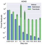
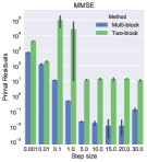
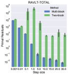
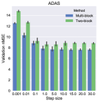
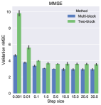
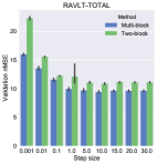
Figure 2: Comparison of two-block and multi-block ADMM for TS-MTL formulation on ADNI-2. Validation nMSE and primal residual are computed as the average over the last 100 iterations of the ADMM. Deviation bars show the variation over 10 independent executions of the methods with different train and test data split.

ADMM with longer training time: A closer observation of Figure 1, particularly the method’s convergence for smaller dual step sizes, $\rho\leq 0.01$, leads to the question whether the two-block ADMM would achieve similar performance to multi-block ADMM if we had continued the optimization process for a longer period of time. To answer this question, we extended the number of iterations for the ADMMs to 10,000 and generated the primal residual curves, as shown in Figure 3. We observe that even for relatively small step sizes ($\rho=0.001$) the two-block ADMM still presents the same unstable behavior for MMSE and RAVLT-TOTAL cognitive scores. For ADAS, the two-block variant shows a slower convergence rate than the multi-block ADMM.

$\boldsymbol{\rho}=0.001$	$\boldsymbol{\rho}=0.01$	$\boldsymbol{\rho}=0.1$

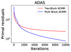
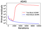
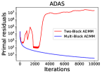
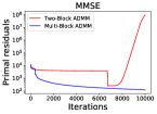
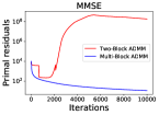
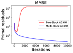
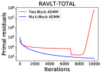
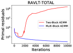
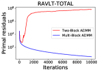
Figure 3: Average curves of primal residuals over 10 executions for all three cognitive scores with longer training time (10,000 iterations) for the ADNI dataset. Multi-block shows a better convergence than two-block ADMM.

Prediction Performance: The final quantitative performance of the multitask learning regressors is measured by their performance on the held-out (test) data set. Table 3 reports the rMSE per task (time point) and nMSE for the three cognitive scores investigated on ADNI dataset. To compute the prediction performance, we used the step size that led to the lowest nMSE on the validation set.

Table 3: Prediction performance results of the three cognitive scores using the dataset ADNI. Multi-block ADMM produced more accurate predictions than the two-block version for all cognitive scores on both nMSE and rMSE.

		ADAS			MMSE			RAVLT-TOTAL
Time points		Two-Block	Multi-Block		Two-Block	Multi-Block		Two-Block	Multi-Block
nMSE		6.48$\pm$0.21	5.09$\pm$0.26		2.81$\pm$0.08	2.24$\pm$0.08		8.99$\pm$0.25	7.22$\pm$0.25
BL   rMSE		6.94$\pm$0.21	6.39$\pm$0.21		2.34$\pm$0.11	2.23$\pm$0.06		9.66$\pm$0.34	9.20$\pm$0.41
M6   rMSE		7.54$\pm$0.36	6.74$\pm$0.21		2.34$\pm$0.11	2.23$\pm$0.06		9.97$\pm$0.49	9.26$\pm$0.31
M12 rMSE		8.71$\pm$0.60	7.64$\pm$0.52		3.41$\pm$0.20	2.97$\pm$0.18		10.92$\pm$0.36	9.62$\pm$0.37
M24 rMSE		9.92$\pm$0.54	9.15$\pm$0.69		4.20$\pm$0.31	3.71$\pm$0.27		11.82$\pm$0.28	10.39$\pm$0.31
M36 rMSE		9.24$\pm$0.35	7.94$\pm$0.44		3.38$\pm$0.29	3.11$\pm$0.19		10.58$\pm$0.62	9.03$\pm$0.40
M48 rMSE		11.50$\pm$1.85	7.59$\pm$1.12		5.74$\pm$0.56	3.64$\pm$0.62		15.12$\pm$1.69	10.70$\pm$0.66

Reflecting the performance on the validation set, the multitask learning formulation optimized by the multi-block ADMM produced lower error on the test set. The improvement is noticed for all cognitive scores and time points (tasks), but is more pronounced in the last time points (M36 and M48), which contains the smallest amount of samples. These results reaffirm the superior performance of the multi-block over the two-block ADMM in our multitask learning formulation for the Alzheimer’s Disease progression problem.

5.2 Parkinson’s disease assessment

For this experiment, we used data from the Parkinson’s Progression Marker Initiative (PPMI) repository. The dataset includes information from healthy individuals and patients diagnosed with Parkinson’s disease. Biospecimen and demographics information are collected from all patients at the beginning of the study, which is referred to baseline (BL), and cognitive assessments are performed in each scheduled visit. Subject’s cognitive function is measured by the MDS-UPDRS-Total score. Not all patients attended all visits, causing some time steps to have a smaller amount of patients. Table 4 shows the number of patients which had their cognitive state assessed at each visit.

Table 4: Parkinson’s dataset: Number of patients (samples) at each time step (task). MX correspond to the number of months X after the baseline screening was taken.

Baseline	Months after baseline
	M3	M6	M9	M12	M18	M24	M30	M36	M42	M48	M54	M60	M72	M84
185	99	99	90	199	97	195	92	209	92	216	80	214	121	82

A set of biological specimens are used to predict the cognitive state of the patient at a certain time in the future (visits). These variables have been identified in the literature as potential biomarkers for Parkinson’s disease progression [37] and [38]. The variables used are listed below.

Cerebrospinal Fluid:

ABeta 1-42, pTau, tTau, CSF Alpha-synuclein, p-tau/t-tau, p-tau/Abeta 1-42, and t-tau/Abeta 1-42.

Plasma:

Total Cholesterol, HDL, Triglycerides, Apolipoprotein A1, LDL, and EGF ELISA.

Serum:

Serum IGF-1.

RNA:

UBC, DJ-1, SNCA-3UTR-2, RPL13, FBXO7-001, SNCA-3UTR-1, DHPR, GLT25D1, FBXO7-007, MON1B, SNCA-E4E6, SNCA-007, FBXO7-005, SRCAP, FBXO7-010, ZNF746, GUSB, SNCA-E3E4, and FBXO7-008.

Besides the biospecimen variables, we include demographics information which may be relevant for the prediction task. Four variables are incorporated: race, family history, gender, and age. Family history is a binary variable informing whether any family member has been diagnosed with PD.

Based on the patients information at the BL time step, the goal is to predict patient’s cognitive function at the following time-steps (visits). Therefore, a predictive model with sparsity structures will be able to identify the variables that most explain the evolution of patient’s cognitive functions. From the multitask learning perspective, predicting the MDS-UPDRS-Total score for each time step (visit) is considered as a task.

We compared the performance of TS-MTL with two-block and multi-block ADMM for several values for the dual step size $\rho$ and the results are showed in Figure 4. It is worth mentioning that the two-block ADMM diverged for $\rho>1$, while multi-block ADMM converged for larger values of $\rho$. We notice that multi-block ADMM achieved consistently lower validation nMSE for the entire range for the dual step size $\rho$. Multi-block primal residuals are significantly smaller for $\rho$ that led to best validation nMSEs ($\rho=0.5$ and $\rho=1$).

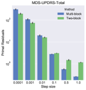
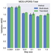
Figure 4: Comparison of two-block and multi-block ADMM for TS-MTL formulation on Parkinson’s disease dataset. Validation nMSE and primal residual are computed as the average over the last 100 iterations of the ADMM. Deviation bars show the variation over 10 independent executions of the methods with different train and test data split.

Convergence curves for both ADMM methods on PD dataset are shown in Figure 5. Notably, multi-block ADMM achieved lower primal residuals and validation nMSE. For $\rho=0.5$ and $\rho=1$, two-block ADMM stagnates and could not longer reduce primal residual and validation nMSE. It is highly probable that even if more iterations were performed, the two-block ADMM would not obtain results comparable to the multi-block version.

$\boldsymbol{\rho}=0.01$	$\boldsymbol{\rho}=0.5$	$\boldsymbol{\rho}=1$

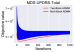
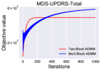
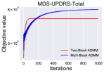
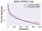
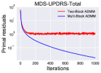
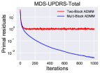
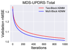
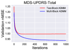
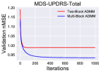
Figure 5: Average curves of objective function, primal residuals, and validation nMSE over 10 executions on the Parkinson’s disease dataset. Many values for learning rate $\rho$ were investigated. Multi-block shows a better convergence than two-block ADMM.

5.3 Air quality prediction

For the Air quality dataset the goal is to predict CO concentration for a certain hour of the day given measurements from 5 distinct sensors + temperature and humidity information. In this setup, we train one regression model for each hour of the day. Although the 24-th hour is connected to 1st hour of the next day, we are not considering this circular dependence for this experiment.

Similar to the other datasets, we conducted experiments with TS-MTL using both two-block and multi-block ADMM for several values of the dual step size $\rho$, and the results are presented in Figures 6 and 7. Again, multi-block shows a steady reduction of primal residuals during optimization, along with a more stable validation performance curves. Although multi-block does not present significant lower nMSE on the validation set in the range of values for $\rho\in[1e^{-4},1e^{-2}]$, it is clearly better for larger values (Figure 6 bottom).

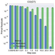
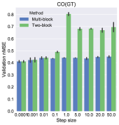
Figure 6: Comparison of two-Block and multi-Block ADMM for TS-MTL formulation on Air Quality data. Multi-block shows similar or better performance than two-block ADMM.

$\boldsymbol{\rho}=0.001$	$\boldsymbol{\rho}=0.01$	$\boldsymbol{\rho}=1$

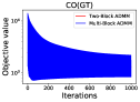
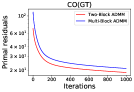
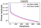
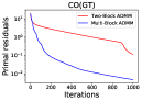
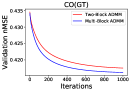
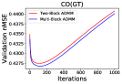
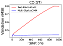
Figure 7: Average curves of objective value, primal residuals, and validation nMSE over 10 executions for Air Quality dataset. Multi-block shows a better convergence than two-block ADMM.

6 Conclusions

In this paper, we reported an experimental study on the convergence aspects of two variants of Alternating Direction Method of Multipliers (ADMM): two-block and multi-block. For many optimization problems associated with data mining and machine learning models, for example, both versions can be used. Given the fact that two-block ADMM has been widely used in the last decade, it has continued to be the method of choice without much thought regarding the use of alternative multi-block ADMM options. For convex problems, they are supposed to give the same solution after all, with suitable choices of (dual) step sizes. However, a question that arises is whether in practice the two-block ADMM is comparable/competitive with multi-block ADMM solving an equivalent problem.

We studied this question in the context of optimization problems arising from multitask learning (MTL) with focus on modeling Alzheimer’s disease (AD) progression, Parkinson’s disease assessment, and air quality prediction. For all three problems, multi-block ADMM showed superior performance when compared to the two-block counterpart, both in terms of convergence stability and prediction power.

Although multi-block ADMM requires further theoretical investigations, we surprisingly showed that in practice it is indeed a candidate to be considered when solving large convex optimization problems if using ADMM. Therefore, we suggest that researchers and practitioners to try out the equivalent multi-block versions of the two-block ADMM and then compare their performance.

Additional, both theoretical and empirical, results for multi-block ADMM are still necessary to precisely characterize the convergence and performance of multi-block ADMM, and these are the future research steps.

References

- [1] S. Boyd, N. Parikh, E. Chu, B. Peleato, and J. Eckstein. Distributed Optimization and Statistical Learning via the Alternating Direction Method of Multipliers. Foundation and Trends in Machine Learning, pages 1–122, 2011.
- [2] H. Wang and A. Banerjee. Bregman Alternating Direction Method of Multipliers. In Advances in Neural Information Processing Systems (NIPS), pages 2816–2824, 2014.
- [3] G. Ye and X. Xie. Split Bregman method for large scale fused Lasso. Computational Statistics & Data Analysis, 55(4):1552–1569, 2011.
- [4] B. Wahlberg, S. Boyd, M. Annergren, and Y. Wang. An ADMM algorithm for a class of total variation regularized estimation problems. IFAC Proceedings Volumes, 45(16):83–88, 2012.
- [5] J. Yang and Y. Zhang. Alternating direction algorithms for L1-problems in compressive sensing. SIAM Journal on Scientific Computing, 33(1):250–278, 2011.
- [6] W. Deng, M. Lai, Z. Peng, and W. Yin. Parallel Multi-Block ADMM with O(1/ k) Convergence. Journal of Scientific Computing, 71(2):712–736, May 2017.
- [7] B. He, M. Tao, and X. Yuan. Alternating direction method with Gaussian back substitution for separable convex programming. SIAM Journal on Optimization, 22(2):313–340, 2012.
- [8] E. Hu and J.T. Kwok. Efficient Kernel Learning from Side Information Using ADMM. In IJCAI, pages 1408–1414, 2013.
- [9] P. Das, N. Johnson, and A. Banerjee. Online lazy updates for portfolio selection with transaction costs. In AAAI, 2013.
- [10] H. Wang, A. Banerjee, and Z. Luo. Parallel direction method of multipliers. In Advances in Neural Information Processing Systems (NIPS), pages 181–189, 2014.
- [11] C. Chen, B. He, Y. Ye, and X. Yuan. The direct extension of ADMM for multi-block convex minimization problems is not necessarily convergent. Mathematical Programming, 155(1-2):57–79, 2016.
- [12] Y. Wang, W. Yin, and J. Zeng. Global convergence of ADMM in nonconvex nonsmooth optimization. arXiv preprint arXiv:1511.06324, 2015.
- [13] F. Wang, W. Cao, and Z. Xu. Convergence of multi-block Bregman ADMM for nonconvex composite problems. arXiv preprint arXiv:1505.03063, 2015.
- [14] T. Lin, S. Ma, and S. Zhang. On the sublinear convergence rate of multi-block ADMM. Journal of the Operations Research Society of China, 3(3):251–274, 2015.
- [15] X. Wang, M. Hong, S. Ma, and Z. Luo. Solving multiple-block separable convex minimization problems using two-block alternating direction method of multipliers. arXiv preprint arXiv:1308.5294, 2013.
- [16] V. Klee and G.J. Minty. How good is the simplex algorithm. Technical report, Washington University Seattle.. Dept of Mathematics, 1970.
- [17] D. P Kingma and J. Ba. Adam: Amethod for stochastic optimization. In International Conference on Learning Representations, 2014.
- [18] D. A Spielman and S. Teng. Smoothed analysis of algorithms: Why the simplex algorithm usually takes polynomial time. Journal of the ACM (JACM), 51(3):385–463, 2004.
- [19] S.S. Du, X. Zhai, B. Poczos, and A. Singh. Gradient Descent Provably Optimizes Over-parameterized Neural Networks. arXiv:1810.02054 [cs, math, stat], 2018.
- [20] S.S. Du, J.D. Lee, H. Li, L. Wang, and X. Zhai. Gradient Descent Finds Global Minima of Deep Neural Networks. arXiv:1811.03804 [cs, math, stat], 2018.
- [21] D. Zou, Y. Cao, D. Zhou, and Q. Gu. Stochastic Gradient Descent Optimizes Over-parameterized Deep ReLU Networks. arXiv:1811.08888 [cs, math, stat], November 2018.
- [22] A. Brutzkus, A. Globerson, E. Malach, and S. Shalev-Shwartz. SGD Learns Over-parameterized Networks that Provably Generalize on Linearly Separable Data. arXiv:1710.10174 [cs], 2017.
- [23] M. Hong, T. Chang, X. Wang, M. Razaviyayn, S. Ma, and Z. Luo. A block successive upper bound minimization method of multipliers for linearly constrained convex optimization. arXiv preprint arXiv:1401.7079, 2014.
- [24] M. Hong and Z. Luo. On the linear convergence of the alternating direction method of multipliers. Mathematical Programming, 162(1):165–199, 2017.
- [25] T. Lin, S. Ma, and S. Zhang. Iteration complexity analysis of multi-block admm for a family of convex minimization without strong convexity. Journal of Scientific Computing, 69(1):52–81, 2016.
- [26] N. Parikh, S. Boyd, et al. Proximal algorithms. Foundations and Trends in Optimization, 1(3):127–239, 2014.
- [27] M. Hong, Z. Luo, and M. Razaviyayn. Convergence analysis of alternating direction method of multipliers for a family of nonconvex problems. SIAM Journal on Optimization, 26(1):337–364, 2016.
- [28] Xiaoli Liu, Peng Cao, André R. Gonçalves, Dazhe Zhao, and Arindam Banerjee. Modeling alzheimer’s disease progression with fused laplacian sparse group lasso. ACM Trans. Knowl. Discov. Data, 12(6):65:1–65:35, 2018.
- [29] L. Wasserman. All of Nonparametric Statistics. Springer-Verlag New York, 2006.
- [30] L. Yuan, J. Liu, and J. Ye. Efficient Methods for Overlapping Group Lasso. IEEE Transactions on Pattern Analysis and Machine Intelligence, 35(9):2104–2116, 2013.
- [31] Y. L. Yu. Better approximation and faster algorithm using the proximal average. In Advances in Neural Information Processing Systems (NIPS), pages 458–466, 2013.
- [32] Y. L. Yu. On decomposing the proximal map. In Advances in Neural Information Processing Systems (NIPS), pages 91–99, 2013.
- [33] A. Argyriou, T. Evgeniou, and M. Pontil. Convex multi-task feature learning. Machine Learning, 73(3):243–272, 2008.
- [34] J. Zhou, J. Liu, V. A. Narayan, J. Ye, and Alzheimer’s Disease Neuroimaging Initiative. Modeling disease progression via multi-task learning. NeuroImage, 78:233–248, 2013.
- [35] J. Wan, Z. Zhang, B. D. Rao, S. Fang, J. Yan, A. J. Saykin, L. Shen, and Alzheimer’s Disease Neuroimaging Initiative. Identifying the Neuroanatomical Basis of Cognitive Impairment in Alzheimer’s Disease by Correlationand Nonlinearity-Aware Sparse Bayesian Learning. IEEE Transactions on Medical Imaging, 33(7):1475–1487, 2014.
- [36] H. Wang, F. Nie, H. Huang, J. Yan, S. Kim, S. Risacher, A. Saykin, and L. Shen. High-Order Multi-Task Feature Learning to Identify Longitudinal Phenotypic Markers for Alzheimer’s Disease Progression Prediction. In Advances in Neural Information Processing Systems (NIPS), 2012.
- [37] S. Khoo, D. Petillo, U. Kang, J. H. Resau, B. Berryhill, J. Linder, L. Forsgren, L.A. Neuman, and A. Tan. Plasma-based circulating microrna biomarkers for parkinson’s disease. Journal of Parkinson’s disease, 2(4):321–331, 2012.
- [38] L. Parnetti, A. Castrioto, D. Chiasserini, E. Persichetti, N. Tambasco, O. El-Agnaf, and P. Calabresi. Cerebrospinal fluid biomarkers in parkinson disease. Nature Reviews Neurology, 9(3):131, 2013.