Two Types of Solar Confined Flares

Abstract

With the aim of understanding the physical mechanisms of confined flares, we selected 18 confined flares during 2011-2017, and classified the confined flares into two types based on their different dynamic properties and magnetic configurations. “Type I” of confined flares are characterized by slipping reconnection, strong shear, and stable filament. “Type II” flares have nearly no slipping reconnection, and have a configuration in potential state after the flare. Filament erupts but is confined by strong strapping field. “Type II” flares could be explained by 2D MHD models while “type I” flares need 3D MHD models. 7 flares of 18 ($\sim$39 %) belong to “type I” and 11 ($\sim$61 %) are “type II” confined flares. The post-flare loops (PFLs) of “type I” flares have a stronger non-potentiality, however, the PFLs in “type II” flares are weakly sheared. All the “type I” flares exhibit the ribbon elongations parallel to the polarity inversion line (PIL) at speeds of several tens of km s^-1. For “type II” flares, only a small proportion shows the ribbon elongations along the PIL. We suggest that different magnetic topologies and reconnection scenarios dictate the distinct properties for the two types of flares. Slipping magnetic reconnections between multiple magnetic systems result in “type I” flares. For “type II” flares, magnetic reconnections occur in anti-parallel magnetic fields underlying the erupting filament. Our study shows that “type I” flares account for more than one third of the overall large confined flares, which should not be neglected in further studies.

1 Introduction

Solar flares are among the most energetic phenomena in the solar atmosphere filled with magnetized plasma. They are often associated with coronal mass ejections (CMEs), which are the dominant contributor to adverse Space Weather at Earth (e.g., Gosling et al. 1991). It is widely believed that the flares and CMEs are two manifestations of the same underlying physical processes. The flares associated with a CME are usually referred to be eruptive events, while the flares that are not accompanied by a CME are called confined events (Svestka & Cliver 1992). Although confined flares have no influence on our space weather conditions, the better understanding of confined flares helps to reveal the physical mechanism of flares and their relationship with CMEs.

The process of eruptive two-ribbon flares is usually described by the CSHKP model (Carmichael 1964; Sturrock 1966; Hirayama 1974; Kopp & Pneuman 1976) and its extension in three dimensions (3D, Aulanier et al. 2012; Janvier et al. 2014). In the CSHKP model, magnetic energy is stored in sheared magnetic arcades or a core flux rope above the polarity inversion line (PIL). Due to the loss of equilibrium, the core magnetic flux system (sheared or twisted) starts to move upward and stretches the embedding magnetic fields. Thus the current sheet is formed underlying the rising core magnetic flux system, and magnetic reconnection occurring in the current sheet releases large amounts of energy via a reconfiguration of the magnetic connectivity. The accelerated particles propagate along the reconnected field lines towards the denser lower atmosphere and generate flare loops and ribbons. As the magnetic reconnection goes on, the reconnection sites are ascending and the flare ribbons are widely observed to separate from each other perpendicularly to the PIL. The erupting core magnetic flux system propels plasma into the interplanetary space and forms a CME.

In the classical two-dimensional (2D) scenario, the preferred sites for the formation of current sheets are the topological features such as magnetic null points and separatrix, which highlight discontinuities in magnetic connectivity (Priest & Forbes 2002). Different from the 2D mode, magnetic reconnection in three dimensions (3D) can also occur at the regions of very strong magnetic connectivity gradients, i.e., quasi-separatrix layers (QSLs, Démoulin et al. 1996; Chandra et al. 2011). The close correspondence between flare ribbons and the photospheric signature of QSLs has been shown in many studies (Schmieder et al. 1997; Masson et al. 2009; Zhao et al. 2014; Savcheva et al. 2015; Yang et al. 2015), which provides a strong evidence for the QSL reconnection. When magnetic reconnection occurs along the QSL, magnetic connectivity is continuously exchanged between neighboring field lines, and the magnetic field lines are observed to “slip” inside the plasma, named slipping reconnection in sub-Alfvénic regime (Priest & Démoulin 1995; Aulanier et al. 2006). In recent years, the standard 3D flare model has been proposed to interpret the intrinsic 3D nature of eruptive flares (Aulanier et al. 2012; Janvier et al. 2014). In this model, the magnetic flux rope is surrounded by the QSLs and the current layer forms along the QSLs. The magnetic reconnection occurs below the erupting flux rope when the current layer at the QSL becomes thin enough, and the flare ribbons coincide with the double J-shaped QSL footprints. Recent high-quality imaging and spectroscopic observations have revealed the signatures of QSL reconnections during eruptive flares (Dudík et al. 2014, 2016; Li & Zhang 2015; Zheng et al. 2016; Gou et al. 2016; Li et al. 2016; Jing et al. 2017). The flare loops were observed to slip along the developing flare ribbons at speeds of several tens of km s^-1 (Dudík et al. 2014, 2016). Two flare ribbons exhibited the elongation motions in opposite directions along the polarity inversion line (Li & Zhang 2014), and the ribbon substructures were seen to undergo a quasi-periodic slipping motion along the ribbon (Li & Zhang 2015).

For confined flares, the key question is the factor determining the confined character of solar flares. Wang & Zhang (2007) analyzed eight X-class flares and found that the confined events occur closer to the magnetic center and the eruptive events tend to occur close to the edge of active regions (ARs), implying that the strong external field overlying the AR core is probably the main reason for the confinement. Similar results have been found by Baumgartner et al. (2018) based on a statistical analysis of 44 flares during 2011-2015. Amari et al. (2018) suggested that the role of the magnetic cage crucially affects the class of eruption$-$either confined or eruptive. To date, many studies have made the consistent conclusion that the decay index of the potential strapping field determines the likelihood of ejective/confined eruptions (Green et al. 2002; Shen et al. 2011; Yang et al. 2014; Thalmann et al. 2015; Chen et al. 2015; Li et al. 2018a). Previous studies showed that the torus instability of a magnetic flux rope occurs when the critical decay index reaches 1.5 (Bateman 1978; Kliem & Török 2006). Zuccarello et al. (2015) performed a series of numerical magnetohydrodynamics (MHD) simulations to flux rope eruptions and found that the critical decay index for the onset of the torus instability lies in a range of 1.3-1.5. Another factor determining whether a flare event is CME-eruptive or not is the non-potentiality of ARs including the free magnetic energy, relative helicity, and magnetic twists (Falconer et al. 2002, 2006; Nindos & Andrews 2004; Tziotziou et al. 2012). Sun et al. (2015) suggested that AR eruptiveness is related to relative value of magnetic non-potentiality over the constraint of background field. However, in the statistical study of Jing et al. (2018), the unsigned twist number of magnetic flux rope plays little role in differentiating between confined and ejective flares and the decay index of the potential strapping field above the flux rope well discriminates them.

In recent years, abundant observations of solar flares show that some flares are not consistent with the classical flare models. This kind of atypical flares has been investigated by several case studies. Liu et al. (2014) carried out the first topological study of an “unorthodox” X-class confined flare exhibiting a cusp-shaped structure, and concluded that the QSL reconnections at the T-type hyperbolic flux tube above the flux rope result in the dynamics of nested loops within the cusp. In the study of Dalmasse et al. (2015), the atypical confined flare was caused by multiple and sequential magnetic reconnections occurring in a complex magnetic configuration of several QSLs. In the recent paper of Joshi et al. (2019), they presented another case study of an atypical confined flare and found that a curved magnetic polarity inversion line of the AR is a key ingredient for producing the atypical flares. However, all of these works are case studies and it is not clear about the physical characteristics and reconnection process of atypical confined flares due to the lack of statistical studies.

In our study, we carry out a statistical analysis of 18 confined flares larger than M5.0 class during 2011-2017. Based on the flare dynamics and extrapolated coronal magnetic fields, we first classify the confined flares into two types. In “type I” confined flares, multiple slipping magnetic reconnections occur in a complex magnetic configuration along two or more QSLs overlying the core magnetic structure, and the entire magnetic system involved in the flare still remains stabilized. “Type II” has the magnetic configuration consistent with the classical flare models, but strong strapping fields are present over the flaring region in the high atmosphere. The structure of the paper is as follows. In Section 2, we describe our event sample and the extrapolated method. Section 3 presents the detailed analysis for three events as typical examples. Finally, in Section 4 we discuss our results and conclude in Section 5.

2 Observations and Data Analysis

In this study, we examined the Geostationary Operational Environmental Satellite (GOES) soft X-ray (SXR) flare catalog to search for flare events larger than M5.0 within $45^{\circ}$ from the disk center in the period from 2011 January to 2017 December. For each event, the CME catalog (Gopalswamy et al. 2009) of the Solar and Heliospheric Observatory (SOHO)/Large Angle and Spectrometric Coronagraph (LASCO) was checked to determine whether the flare was confined or not. We regarded a flare as confined if there is no CME within 60 min of the flare start time in the quadrant consistent with the flare position. In addition, we also visually inspected the Solar Dynamics Observatory (SDO; Pesnell et al. 2012) and the twin Solar Terrestrial Relations Observatory (STEREO; Kaiser et al. 2008; Howard et al. 2008) observations to further verify the classification of eruptive and confined flares. A total of 18 confined flares from 12 ARs fulfilled the selection criteria above (see Table 1).

To analyze the structure and dynamics of each confined flare, we used the E(UV) observations from the Atmospheric Imaging Assembly (AIA; Lemen et al. 2012) on board the SDO, with a resolution of $\sim$0$\arcsec$.6 per pixel and a cadence of 12/24 s. Four channels of AIA 1600, 304, 171, and 131 Å were mainly applied to classify these confined flares. The topology of the magnetic fields of the AR is important to interpret the development of the flare. Thus we performed the nonlinear force-free field (NLFFF) extrapolations (Wheatland et al. 2000; Wiegelmann 2004) to the selected events and obtained their 3D source coronal magnetic fields. The vector magnetogram used as the bottom boundary condition (z=0) for the extrapolations was an Helioseismic and Magnetic Imager (HMI; Scherrer et al. 2012) data product called Space-Weather HMI AR Patches (Bobra et al. 2014). The vector magnetogram was pre-processed to remove the net force and torque on the photospheric boundary (Wiegelmann et al. 2006). We also calculated the squashing factor (Q) and twist number based on the extrapolated 3D magnetic fields with the code introduced by Liu et al. (2016b). The QSL distribution can be quantified by the Q factor, which measures the magnetic field connectivity gradient by tracing field lines pointwise (Titov et al. 2002).

3 Results

We looked through the AIA 1600, 304, 171, and 131 Å movies for all the 18 confined flares, and found that our events could be categorized into two groups:

“Type I” flares.-The common characteristic among all the flares in this group is that the flaring structure is complex with two or more sets of magnetic systems, and it is not associated with any eruption of core filament. The post-flare loops (PFLs) are strongly sheared with respect to the PIL of the AR and they are overlying the non-eruptive filament.

“Type II” flares.-The flares in this group are associated with the failed eruption of a core filament, and have the weakly sheared PFLs underlying the erupting filament. Large-scale strapping loop bundles overlying the flaring region could be seen in high-temperature wavelengths (131 and 94 Å) during the development of the flare. In other words, this group of flares are consistent with the classical flare models.

According to the classification criteria of confined flares, 7 flares of 18 ($\sim$39 %) belong to “type I” and 11 ($\sim$61 %) are “type II” confined flares (see Table 1). Two events of “type I” and one event of “type II” are taken as examples to analyze the flare dynamics and magnetic topological structures in detail.

3.1 “Type I”: the X1.5-class Flare on 2011 March 09

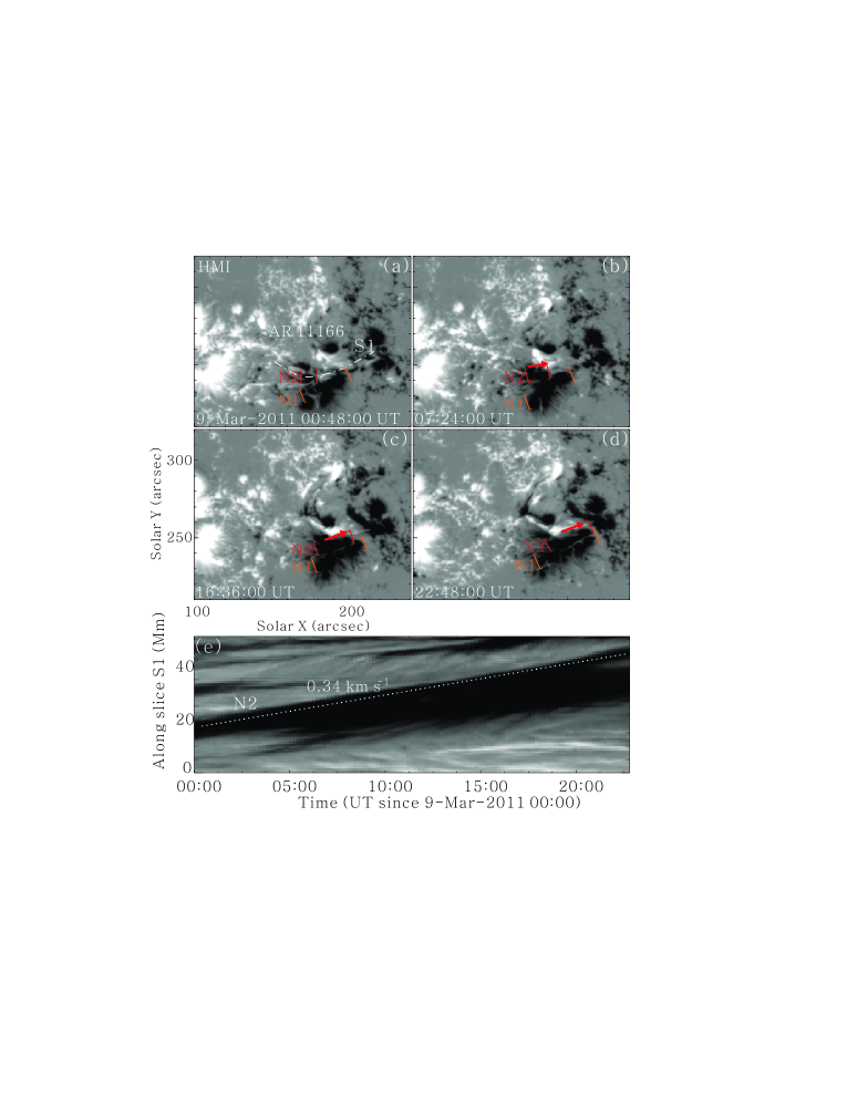
Figure 1: Temporal evolution of the HMI LOS magnetic field (saturating at $\pm$1000 G) prior to the X1.5-class flare on 2011 March 09. Negative patch N1 is the formerly existed magnetic flux and negative patch N2 is new emerging flux. White dash-dotted curve “S1” in panel (a) represents the location used to obtain the stack plot shown in panel (e). Red arrows in panels (b)-(d) indicate the shearing motion of the emerging flux N2. White dotted line in panel (e) denotes the shearing motion of N2 along slice “S1”. The FOV of panels (a)-(d) is the same as Figure 2.

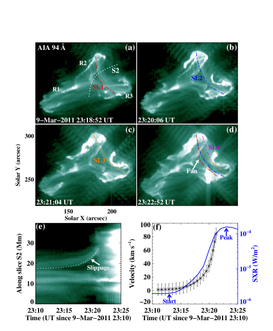
Figure 3: Apparent slipping motion of flare loops in the impulsive phase of the flare. Panels (a)-(d): time series of 94 Å images showing the slipping flare loops connecting ribbons R2 and R3. Dash-dotted curves (SL1-SL4) traced the easternmost part of the slipping loop bundles. These successively visible loop structures (SL1-SL4) delineated a “fan-shaped surface” shown in panel (d). White dotted curve “S2” in panel (a) denotes the location used to obtain the stack plot shown in panel (e). Panels (e)-(f): stack plot along slice “S2” and the velocity-time profile (black curve) showing the acceleration process of the slipping motion. The uncertainty of the speed was estimated to be about 8.5 km s^-1 due to the uncertainty in the height measurement of 2 pixels. The blue curve in panel (f) is the GOES SXR 1$-$8 Å flux variation.

One selected event of “type I” confined flares is the X1.5-class event occurring in AR 11166 near the solar disk center (N$08^{\circ}$, W$11^{\circ}$) on 2011 March 09. The GOES soft X-ray 1$-$8 Å flux showed that the X1.5-class flare initiated at 23:13 UT and reached its peak at 23:23 UT (Figure 3(f)). Line-of-sight (LOS) magnetograms from the HMI on board the SDO are used to investigate the evolution of photospheric magnetic fields before the flare. The evolution of the AR presented localized magnetic flux emergence and strong shearing motions as displayed in Figure 1. The new negative-polarity patch N2 emerged nearby the pre-existing negative-polarity patch N1 about one day before the flare onset. Simultaneously, the emerging patch N2 showed a strong shearing motion towards the northwest, together with a weak shear of pre-existing patch N1 along the same direction with N2. Along the shearing direction of patch N2 (white dash-dotted curve “S1” in Figure 1(a)), we obtain a stack plot (Figure 1(e)) based on the 12-min LOS magnetograms. The average shearing speed of emerging patch N2 was about 0.34 km s^-1, comparable to the statistical results showing that the maximum shear-flow speeds of the above M1.0 flaring-AR have a peak value of 0.3$-$0.4 km s^-1 (Park et al. 2018; Hou et al. 2018).

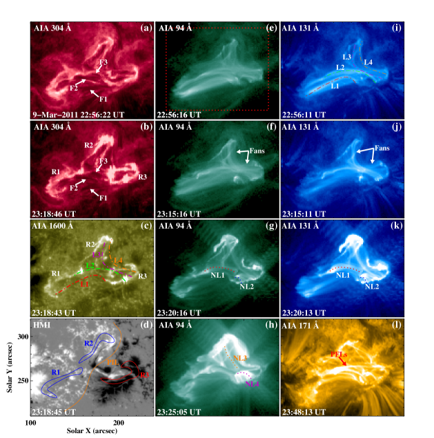
Figure 2: Appearance of the X1.5-class flare on 2011 March 09 in different (E)UV wavelengths and the corresponding LOS magnetogram from the SDO/AIA and SDO/HMI. F1-F3 in panels (a)-(b) are three non-eruptive filaments at the flaring region. R1-R3 in panels (b)-(d) denote three flare ribbons and they are outlined by blue and red contours in panel (d). The orange curve in panel (d) indicates the average orientation of the polarity inversion line (PIL) of the AR obtained from the HMI LOS magnetogram. The red dotted rectangle in panel (e) denotes the FOV of Figures 3(a)-(d). L1-L4 in panels (c) and (i) are four brightened loop bundles identified in 131 Å prior to the flare. NL1-NL4 in panels (g)-(h) and (k) denote newly formed loop bundles during the flare. PFLs in panel (l) represents post-flare loops in the low-temperature channel of 171 Å after the flare. The animation of this figure includes AIA 304, 171, 94 and 131 Å images from 22:30 UT to 24:00 UT. The video duration is 37 s.

At the flaring region, three filaments F1-F3 existed between the positive and negative magnetic fluxes (Figures 2(a) and (d)). Their lengths are about 10-30 Mm, belonging to the category of mini-filaments (Hermans & Martin 1986; Hong et al. 2017). During the flare process, these filaments did not show the rise phase and were not associated with any failed eruptions. They were stably present after the flare and seemed not to be affected by the evolution of the flare (Figure 2(b)). For “type I” confined flares, high-temperature flare loops displayed significant dynamic evolution, and thus AIA 94 and 131 Å observations (about 7 MK for 94 Å and 11 MK for 131 Å; O’Dwyer et al. 2010) were analyzed in detail. From about 22:47 UT ($\sim$26 min before the flare onset), the flare loops started to be illuminated in 131 Å channel indicating the initiation of magnetic reconnections. We identified two sets of bright loop bundles labeled L1-L4 in the hot line (131 Å) at 22:56 UT (Figure 2(i)), displaying two different magnetic connectivities. These loop bundles can not be clearly discerned in 94 Å (Figure 2(e)), meaning that their temperature is around 10 MK. As the flare developed, more flare loops appeared and delineated “fan-shaped surfaces” (Figures 2(f) and (j)). At about 23:20 UT, new loop bundles NL1 and NL2 were formed (Figures 2(g) and (k)), implying the reconfiguration of magnetic fields caused by magnetic reconnections. Later on, the 94 Å observations showed the formation of another two loop bundles NL3 and NL4 at 23:25 UT (Figure 2(h)). The PFLs detected in the low-temperature line (171 Å at $\sim$0.6 MK) were formed overlying the non-eruptive filaments (Figure 2(l)).

The comparison of the 1600 Å image with HMI LOS magnetogram showed that the flare consisted of two positive-polarity ribbons R1 and R2 and a semi-circular ribbon R3 (Figures 2(c)-(d)). The pre-flare evolution of magnetic fields showed that ribbon R3 was located at the emerging and shearing negative-polarity patch N2 (Figures 1(d) and 2(d)). We overplotted the pre-flare loop bundles L1-L4 of 131 Å on the 1600 Å image and found that their footpoints were perfectly co-spatial with the flare ribbons. The eastern footpoints of loops L1-L2 were located at ribbon R1 and their western footpoints at ribbon R3. The north ends of loops L3-L4 anchored in ribbon R2 and their south ends at ribbon R3. The correspondence of the loop footpoints with the flare ribbons implies that the magnetic reconnections mainly occur in the two sets of magnetic connectivities outlined by loops L1-L4. We suggest that L2 and L3 are reconnecting, then L1 and L4 move toward the reconnection region and reconnect subsequently. During the development of the flare, ribbons R1-R3 did not show any evident separation motion perpendicular to the PIL (orange line in Figure 2(d)). Ribbons R1 and R3 exhibited the elongation motions at their hook parts along the magnetic PIL. Ribbon brightening of R1 spread towards the south and R3 appeared to spread mostly northward at an average speed of 33 km s^-1 (see Table 1).

The flare loops exhibited an apparent slipping motion towards the northwest in the impulsive of the flare in 94 Å channel (Figure 3). From about 23:15 UT, the loop bundle connecting ribbons R2 and R3 was seen to slip. The easternmost loop of the bundle can be clearly discerned (SL1-SL4 in Figures 3(a)-(d)) and thus was used to trace the dynamic evolution of the loop bundle. The south footpoints of the slipping loops SL1-SL4 moved along ribbon R3 to the west, and the displacement of their north footpoints along ribbon R2 was not evident compared with that of the south ends. The morphology of the loops was changed gradually from curved to straight, suggesting that each time it was not the same structure, but a new flare loop. The new flare loop became visible due to the slipping magnetic reconnections, similar to the observations of Li & Zhang (2014, 2015). Eventually, these successively visible loop structures delineated a “fan-shaped surface” (Figure 3(d)). To analyze the slipping motion, we placed an artificial cut “S2” along the slipping direction (white dotted curve in panel (a)). This cut was used to produce the time-distance plot in AIA 94 Å shown in Figure 3(e). As shown from the time-distance plot, the slipping motion exhibited an acceleration process during the flare evolution. By tracing the easternmost loop in the time-distance plot (dotted line in panel (e)), we obtained the velocity-time plot of the slipping motion (black curve in Figure 3(f)). The slippage can be described by two kinematic phases: a slow slipping phase and a fast slipping phase. The slipping motion was slow in the early stage and reached $\sim$11 km s^-1 at about 23:17 UT. Then the apparent slipping speed started to increase impulsively and up to $\sim$84 km s^-1 at about 23:21 UT. We assumed an error of two pixels (1$\arcsec$.2) in the height measurement and the uncertainty in the speed was estimated to be about 8.5 km s^-1. The speed profile of the slippage has a similar trend to the GOES SXR 1$-$8 Å flux variation (blue curve in panel (f)), but with a delay of several minutes.

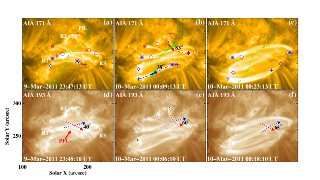
Figure 4: Time series of 171 and 193 Å images showing the morphology of PFLs. Green dash-dotted line is the duplication of the PIL (the orange curve in Figure 2(d)). 38^∘ in panel (b) is the inclination angle between the blue arrow (the tangent of the blue dash-dotted line) and the green arrow (the tangent of the PIL). 83^∘ is the inclination angle between the red dash-dotted curve and the PIL. Blue marks in panels (a)-(c) indicate the footpoints of the measured PFLs connecting ribbons R1 and R3. Red marks denote the footpoints of another set of PFLs connecting ribbons R2 and R3. Red and blue dotted lines in panels (d)-(f) are used to estimate the mutual orientation between the two sets of PFLs.

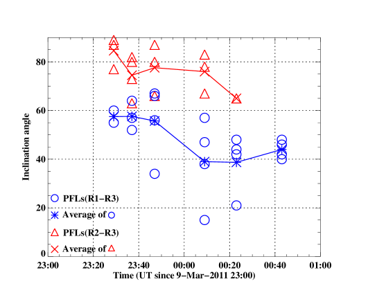
Figure 5: Inclination angles of the observed PFLs with respect to the PIL during the development of the flare. The blue circles denote the inclination angles of the PFLs connecting ribbons R1 and R3, and the blue asterisks are the average angles at the same time. The red symbols are for the PFLs connecting ribbons R2 and R3.

We investigated the development of PFLs in the gradual phase of the flare and estimated the inclination angles of PFLs with respect to the PIL (Figure 4). The average orientation of the PIL is determined from the HMI LOS magnetogram prior to the flare onset. The inclination angle $\theta$ corresponds to the angle between the tangents of the PFL and PIL at their intersection (panel (b)), which is consistent with the method of Zhang et al. (2017). The complementary angle of $\theta$ has been referred to as the shear angle in previous studies (Su et al. 2007; Aulanier et al. 2012). Similar to the pre-flare morphology (Figure 2(i)), the PFLs also exhibited two different magnetic connectivities. One set of PFLs seemed to connect ribbons R2 and R3 (red symbols and red dash-dotted line in panels (a)-(b)), and another overlying set of PFLs connecting R1 and R3 (blue symbols and blue dash-dotted line in panels (a)-(c)). In Figures 4(d)-(e), we measured the mutual orientation between the two sets of PFLs (blue dotted lines connecting ribbons R1 and R3; red dotted lines connecting R2 and R3). The angles (40, 60 and 65^∘) are obtained by measuring the angles between the tangents of red and blue loops. Starting from 23:30 UT, about 35 PFLs have been identified and their $\theta$ values were estimated. Figure 5 shows the results of $\theta$ for these PFLs, separated into two groups according to their connectivity. The set of PFLs connecting R1 and R3 has a higher non-potentiality, e.g., strong shear (or deviating from potential fields). Their $\theta$ values range from 15^∘ to 67^∘ (blue symbols), and the average $\theta$ is about 48^∘ (see Table 1). Another set of PFLs connecting R2 and R3 has larger $\theta$ values of 63^∘-90^∘, implying that they are approximately perpendicular to the PIL and weakly sheared fields.

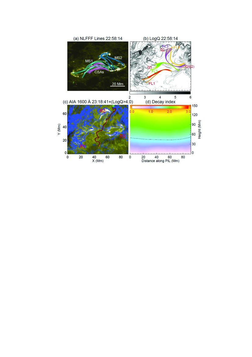
Figure 6: 3D magnetic field structure, QSL and decay index distribution. Panel (a): side view of the extrapolated field lines at 22:58 UT showing two magnetic systems (MS1 and MS2, cyan and blue lines) involved in the flare and the underlying core sheared arcades (CSAs, pink lines). The background is the 1600 Å image showing the locations of flare ribbons. Panel (b): selected four strands of magnetic field lines (FL1-FL4) by comparing with the observed flare loop bundles (L1-L4 in Figure 2(i)) plotted over the distribution of the squashing factor Q on the bottom boundary. FL1-FL2 delineate a QSL structure Q1 and FL3-FL4 outline another QSL structure Q2. Panel (c): overlay between the flare ribbons (underlying 1600 Å image) and the QSL map (blue curves). All regions with Q_thresh$>$10⁴ are shown in this panel. The PIL is extracted from the bottom boundary of the extrapolated NLFFFs and marked by the red curve. The “$\times$” symbol shows the starting point of the PIL. Panels (b)-(c) have the same FOV. Panel (d): distribution of the decay index above the PIL (red curve in panel (c)) prior to the flare onset. The black line marks the positions where decay index n reaches the critical value of 1.5.

Figure 6 displays the coronal magnetic field lines and the photospheric Q-map. The extrapolation results show the existence of two sets of magnetic systems (MS1 and MS2, cyan and blue lines in panel (a)) and the underlying three sets of core sheared arcades (CSAs, pink lines in panel (a)) at the flaring region. MS1 seems to connect ribbons R1 and R3, and MS2 connects ribbons R2 and R3. The surface delineated by MS1 lies below the corresponding surface of MS2, with both of them overlying the CSAs. The three CSAs are strongly sheared with the average twist number of about 0.5-0.7, which probably correspond to the three non-eruptive filaments (F1-F3 in Figure 2(a)). We identified four field line strands (FL1-FL4 in Figure 6(b)) by comparing with the observed high-temperature loop bundles (L1-L4 in Figure 2(i)), and plotted them over the photospheric Q-map (Figure 6(b)). The four strands FL1-FL4 are anchored in the locations with high Q value of about 10⁴-10⁵, indicating the positions of QSLs with strong connectivity gradients. FL1-FL2 delineate a QSL structure labeled Q1, and FL3-FL4 outline another QSL structure Q2 (Figure 6(b)). The overlay between the flare ribbons (underlying 1600 Å image) and the photospheric Q-map is shown in panel (c). We can see that the Q distribution nearby ribbon R1 is very complex and is poorly matched with R1. However, the other two ribbons R2 and R3 have a good correspondence with high Q regions, with R2 residing in the north end of Q2 and R3 in the common west end of Q1 and Q2. The close relations between observed flare ribbons and calculated high Q regions imply that the dominant reconnection process during the flare occurs along the two QSLs. It is noted that not all high-Q regions have corresponding flaring activity. The reason is that in some high-Q regions, no current is accumulated and thus no flaring activity is observed (Savcheva et al. 2015). In order to estimate the magnetic field gradient in the environment of CSAs, we computed the distribution of the decay index n above the PIL prior to the flare onset (Figure 6(d)). The black line marks the position where n reaches the critical value of 1.5 for the onset of torus instability (Kliem & Török 2006). The critical height is above 45 Mm at all portions above the PIL.

3.2 “Type I”: the X2.0-class Flare on 2014 October 26

Another selected event of “type I” confined flares is the X2.0-class flare occurring in the famous AR 12192 on 2014 October 26. AR 12192 was the biggest sunspot region in the solar cycle 24 and produced 6 X-class flares, 22 M-class flares, and 53 C-class flares during its disk passage. The most peculiar aspect of this AR was that all the X-class flares were confined and none of them were associated with CMEs. The famous AR drew considerable attention and has been extensively studied (Thalmann et al. 2015; Sun et al. 2015; Chen et al. 2015; Liu et al. 2016a; Sarkar & Srivastava 2018). They suggested that the weaker non-potentiality and stronger strapping magnetic field resulted in the confinement of the flares. Zhang et al. (2017) analyzed the evolution of four confined X-class flares on 2014 October 22-26 and concluded that the complex magnetic structures are responsible for the confined character of solar flares.

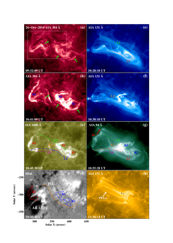
Figure 7: SDO/AIA multi-wavelengths (E)UV images and SDO/HMI LOS magnetogram showing the appearance of the X2.0-class flare in AR 12192 on 2014 October 26. The green arrows in panels (a)-(b) point to the non-eruptive filament along the PIL. The white dotted rectangle in panel (a) denotes the FOV of Figures 8(a)-(c). R1-R3 are three flare ribbons in the central region of the AR, and their brightness contours in 1600 Å are shown in panel (d). The orange curve in panel (d) indicates the average orientation of the PIL of the AR. Dotted curves L1-L4 in panels (e)-(g) outline the four loop bundles identified in 131 and 94 Å, and their duplicates are drawn by dash-dotted lines in panels (c) and (g). The red arrow in panel (g) denotes the elongation motion of ribbon R1. White arrow in panel (h) points to the post-flare loops in 171 Å. The animation of this figure includes AIA 304, 171, 94, and 131 Å images from 10:20 UT to 12:00 UT. The video duration is 25 s.

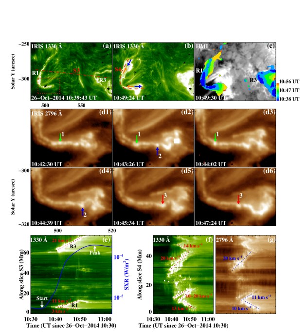
Figure 8: Dynamic evolution of ribbons R1 and R3 from IRIS high-resolution observations. Panels (a)-(b): IRIS 1330 Å images showing flare ribbons R1 and R3. Red dash-dotted line “S3” in panel (a) and dashed curve “S4” in panel (b) respectively denote the locations used to obtain the stack plots shown in panels (e) and (f)-(g). Red dotted rectangle in panel (a) denotes the FOV of panels (d1)-(d6). Orange and blue arrows in panel (b) represent the bi-directional slippage of ribbon R1. Panel (c): SDO/HMI LOS magnetogram with an overlay of the evolving positions of ribbons R1 and R3. The color indicates the time of the ribbon brightness at 10:38-10:56 UT in 1330 Å SJIs. Panels (d1)-(d6): time series of IRIS 2796 Å images showing the slippage of traced bright knots (“1”$-$“3”) within ribbon R1. Bright knots “1” and “3” slipped towards the east and knot “2” slipped in the opposite direction. Panel (e): 1330 Å stack plot along slice “S3” (panel (a)) displaying the motions of R1 and R3 perpendicular to the PIL. Blue curve is the GOES SXR 1-8 Å flux of the flare. Panels (f)-(g): 1330 and 2796 Å stack plots along slice “S4” (panel (b)) showing the bi-directional slippage along ribbon R1. The animation of this figure includes IRIS 1330 and 2796 Å images from 10:00 UT to 11:15 UT. The video duration is 24 s.

A total of 6 flares in AR 12192 satisfied our selection criteria, including 4 X-class flares and 2 M-class flares. The X2.0-class flare on October 26 was analyzed in detail in this study, which has never been investigated thoroughly in previous studies. The X2.0-class flare has the simultaneous high-resolution observations from the Interface Region Imaging Spectrograph (IRIS; De Pontieu et al. 2014) showing clear dynamic evolution of flare ribbons. The onset time of the X2.0-class flare was 10:35 UT and the peak time was 10:56 UT as shown from the GOES SXR 1$-$8 Å flux (Figure 8(e)). The AR was located at the S$10^{\circ}$-$20^{\circ}$ latitude and W$30^{\circ}$-$45^{\circ}$ longitude during the flare. The 304 Å observations showed that a “reverse S-shaped” filament was present along the PIL of the AR, with a length of about 45 Mm (green arrows in Figure 7(a)). After the flare onset, the western part of the filament was activated and associated with EUV brightenings (Figure 7(b)). However, the entire filament did not show any rise phase except for the moderate brightenings and remained stabilized through the flare. Three flare ribbons appeared in the central region of the AR, including one negative-polarity ribbon (R1) in the trailing sunspot of the AR and two positive-polarity ribbons (R2 and R3) anchoring in the periphery of the leading sunspot (Figures 7(c)-(d)). The location and morphology of the flare ribbons in this event are similar to the other five flares in the same AR, implying that they are homologous flares with an analogous triggering mechanism.

High-temperature flare loops exhibited a complicated structure as seen from the 131 and 94 Å observations. Four loop bundles (L1-L4 in panels (e)-(g)) overlying the non-eruptive filament were identified, which were probably involved in the magnetic reconnections of the flare. At 10:28 UT prior to the flare, L1 and L2 showed faint brightenings (panel (e)), indicative of the onset of weak magnetic reconnections. Then at 10:38 UT, a shorter and brighter loop bundle L3 (panel (f)) appeared underlying L1 and L2. Simultaneously, three flare ribbons R1-R3 were formed at the footpoints of the heated flare loops (panel (f)). Associated with the development of the flare, flare loops connecting ribbons R1 and R2 exhibited an apparent slipping motion towards the north along ribbon R1 (red arrow in panel (g)), implying the occurrence of slipping magnetic reconnections. At the peak time of the flare, the southernmost loop L4 connecting ribbons R1 and R3 was seen in the 94 Å channel, and L3-L4 jointly comprised a “triangle-shaped flag surface” (Figures 7(c) and (g)). At last, these high-temperature flare loops gradually cooled down and formed PFLs overlying the non-eruptive filament in 171 Å (panel (h)). We suggest that L1-L2 outline a set of sheared magnetic system and L3-L4 delineate another set of magnetic system. The two systems are interacting and reconnecting with each other, which generates the confined flare.

This flare was also observed by the IRIS slit jaw imagers (SJIs) in 1330 and 2796 Å channels with a spatial pixel size of 0$\arcsec$.33, a field of view (FOV) of 120$\arcsec$$\times$119$\arcsec$ and a cadence of about 18 seconds. Figure 8 shows the observational results from the IRIS, displaying the detailed dynamic evolution of flare ribbons R1 and R3. As seen from the stack plot (Figure 8(e)) along slice “S3” (dash-dotted line in Figure 8(a)) in 1330 Å, ribbons R1 and R3 spread fast perpendicular to the PIL at respective speeds of about 11 km s^-1 and 21 km s^-1 along the same direction. As seen from Table 1, four of six flares in the same AR exhibited the perpendicular motion with respect to the PIL at speeds of 10-21 km s^-1. The ribbon motion is probably controlled by the magnetic environment and the ribbons in some flares can not really move due to strong fields.

In addition to the motions perpendicular to the PIL, bidirectional slipping motion of ribbon R1 along the PIL was also detected (orange and blue arrows in panel (b)). To analyze the slipping motions, we place an hook-shaped cut “S4” (dashed curve in panel (b)) along ribbon R1 and obtained the stack plots in IRIS 1330 and 2796 Å (Figures 8(f)-(g)). The slipping motions were in both directions with speeds of 10-20 km s^-1. These velocities are generally lower than those reported from other flares (Dudík et al. 2014, 2016; Li & Zhang 2015; Li et al. 2018b). The overlay of the flare ribbon time evolution over the magnetogram is displayed in Figure 8(c). The color indicates the time of the ribbon brightness observed in IRIS 1330 Å SJIs. It clearly shows the bidirectional elongations of ribbon R1 and the unidirectional perpendicular expansions of ribbons R1 and R3. Figures 8(d1)-(d6) display the zoomed 2796 Å images of the south part of ribbon R1. As seen from these zoomed images, ribbon R1 was composed of numerous bright knots, which exhibited apparent slipping motions along R1. Three individual bright knots within R1 were tracked (labeled as “1”$-$“3”) at 10:42-10:47 UT. Bright knot “1” slipped towards the east along the straight part of R1, with a displacement of about 2.4 Mm in 1.5 min and an average speed of 27 km s^-1. Bright knot “2” slipped toward the west at a faster speed of about 36 km s^-1. At 10:45:34 UT, another bright knot “3” was traced to slip in the same direction as knot “1”. The elongation motion of flare ribbons parallel to the PIL can also be observed in other five flares of the same AR (see Table 1). The elongation velocity is in the range of 11-45 km s^-1, which is comparable to the previous case and statistical studies (Krucker et al. 2003; Lee & Gary 2008; Qiu et al. 2017).

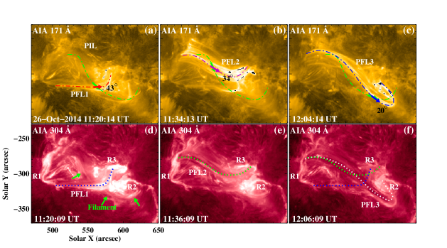
Figure 9: Time series of 171 and 304 Å images showing the sheared PFLs. Green dash-dotted line is the duplication of the PIL (the orange curve in Figure 7(d)). PFL1-PFL3 are three sets of PFLs, appearing successively during the gradual phase of the flare. Three examples of PFLs (red, purple and blue dash-dotted curves in panels (a)-(c)) are shown to estimate their inclination angles with respect to the PIL. Green arrows in panel (d) point to the non-eruptive filament underlying the PFLs. Blue, green and white dotted curves in panels (d)-(f) represent the connectivities of dark arcades between ribbons R1-R3.

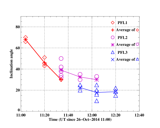
Figure 10: Inclination angles of the observed PFLs with respect to the PIL during the development of the flare. Red symbols denote the inclination angles of the PFL1 and the average values. The purple symbols are for the PFL2, and the blue marks for the PFL3.

Starting from about 11:00 UT, the reconnected flare loops gradually cooled down and formed PFLs in 171 Å (Figures 9(a)-(c)). A set of PFLs (PFL1 in Figure 9(a)) connecting the south part of ribbon R1 and R3 were initially detected. We estimated the inclination angles $\theta$ of PFL1 with respect to the PIL and displayed the measurement results in Figure 10. The PIL in this event is determined according to the position of the non-eruptive filament (Su et al. 2006). PFL1 shows an increasing shear, with the $\theta$ values ranging from 70^∘ to 30^∘ (red symbols in Figure 10). As seen from the 304 Å images, PFL1 appeared as bright and dark alternatively arcades (Figure 9(d)), indicative of the presence of hot and cold materials along the PFLs. PFL1 were overlying the non-eruptive filament (green arrows in Figure 9(d)), implying that the filament did not play any part in the reconnection process. From about 11:28 UT, another set of PFLs (PFL2 in Figures 9(b) and (e)) appeared connecting the north part of ribbon R1 and R3. The inclination angles $\theta$ of PFL2 were in the range of 30^∘-50^∘ (purple symbols in Figure 10), suggesting that PFL2 were strongly sheared loops with respect to the PIL. About 1 hour after the flare peak (11:50 UT), another set of large-scale PFLs were observed connecting ribbons R1 and R2 (PFL3 in Figures 9(c) and (f)). They were nearly parallel to the PIL and had a higher non-potentiality, with the $\theta$ of 10^∘-25^∘ (blue marks in Figure 10). The three sets of PFLs were successively formed and ultimately delineated two groups of magnetic connectivities (Figure 9(f)), similar to the pre-reconnecting high-temperature flare loops (Figure 7). Moreover, the PFLs of the other five flares in the same AR also exhibited a strong shear, with $\theta$ values of 20^∘-45^∘ (see Table 1).

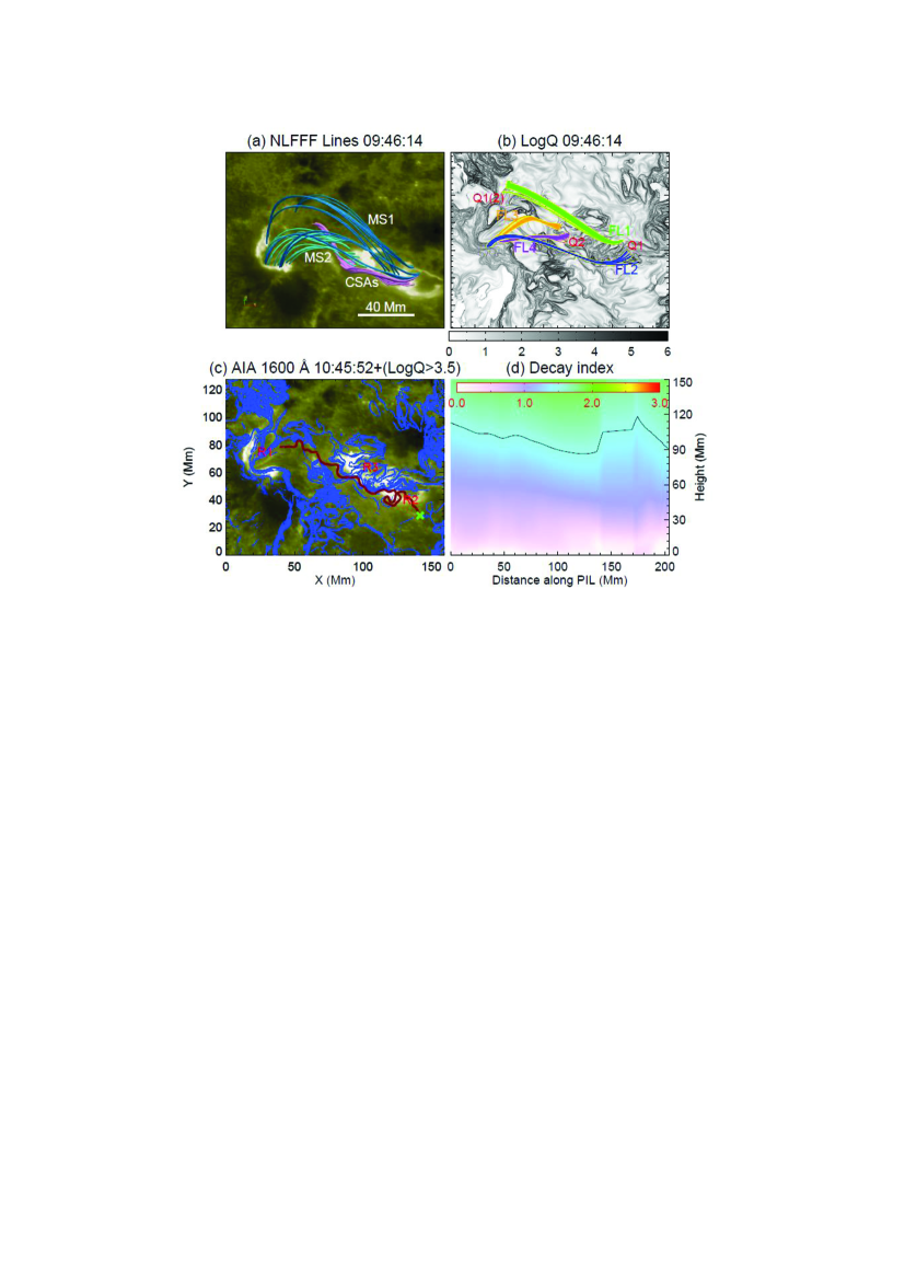
Figure 11: Magnetic field structure, QSL and decay index distribution. Panel (a): 3D structure of the field lines of the NLFFF showing the CSAs (pink lines) and two sets of overlying magnetic systems (MS1 and MS2, blue and cyan lines). Panel (b): selected four strands of field lines (FL1-FL4) plotted over the distribution of the squashing factor Q in the z=0 plane. FL1-FL2 delineate a QSL structure Q1 and FL3-FL4 outline another QSL structure Q2. Panel (c): overlay between the flare ribbons (underlying 1600 Å image) and the QSL map (blue curves). All regions with Q_thresh$>$10^3.5 are shown in this panel. The PIL is extracted from the bottom boundary of the extrapolated NLFFF and marked by the red curve. The “$\times$” symbol shows the starting point of the PIL. Panels (b)-(c) have the same FOV. Panel (d): distribution of the decay index n above the PIL (red curve in panel (c)) prior to the flare onset. The black line marks the positions where decay index n reaches the critical value of 1.5.

Figure 11(a) shows the 3D structure of the magnetic field lines of the NLFFF based on the photospheric vector magnetogram at 09:46 UT. We find that a set of CSAs along the PIL and two sets of sheared magnetic systems (MS1 and MS2) overlying the flux rope are present in the central region of the AR. CSAs consist of weakly twisted field lines with the average twist number of 0.6. Compared to Figure 7, CSAs bear a good resemblance to the observed non-eruptive filament. The east ends of MS1 and MS2 both anchored in ribbon R1 and their respective west ends in two positive-polarity ribbons R2 and R3. The extrapolated magnetic topology of the AR core is approximately consistent with the results of Inoue et al. (2016) and Jiang et al. (2016), who analyzed the X3.1-class flare on October 24 and suggested that the AR was composed of multiple strongly-sheared flux tubes. Based on the observed loop bundles L1-L4 in Figure 7, we select four strands of field lines (FL1-FL4 in Figure 11(b)) and find that their footpoints are located at the regions with high Q value. Thus it is deduced that two QSLs are connected with the flare, which are respectively outlined by FL1-FL2 and FL3-FL4.

The photospheric intersections of the two QSLs (Q1 and Q2) and the brightening ribbons in 1600 Å image (panel (c)) show an approximate correspondence. Ribbon R1 has a similar morphology with the common eastern end of Q1 and Q2, although there is a little displacement between them. The displacement is probably caused by the evolution of QSL structures during the development of the flare. The western two ribbons R2 and R3 are approximately matched with the western ends of Q1 and Q2. Due to the evident evolution of flare ribbons perpendicular to the PIL (Figure 8), the correspondences between pre-flare QSLs and flare ribbons are not as good as the first event on 2011 March 09. We display the distribution of the decay index n above the PIL prior to the flare onset in panel (d). It shows that the decay index n does not reach the critical value of 1.5 until 90 Mm, implying a strong confinement overlying the filament.

3.3 “Type II”: the M5.3-class Flare on 2012 July 04

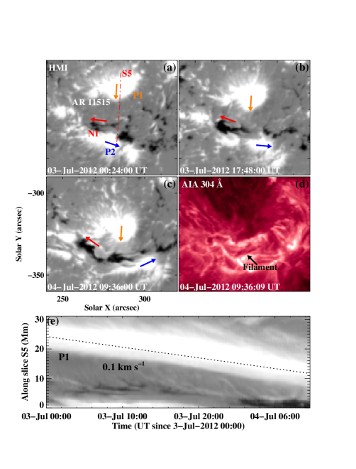
Figure 12: Magnetic field evolution of AR 11515 prior to the M5.3-class flare on 2012 July 04. Panels (a)-(c): SDO/HMI LOS magnetograms (saturating at $\pm$1000 G) showing the photospheric evolution at the flaring region. Orange arrows represent the converging motion of the positive-polarity sunspot P1. Red and blue arrows denote the shearing motions of N1 and P2 in opposite directions. The slice “S5” is drawn as red dash-dotted line in panel (a), for which the time-distance plot is presented in panel (e). Panel (d): SDO/AIA 304 Å image showing the location of the filament before the eruption. Panel (e): time-distance plot along the slice “S5” in the LOS magnetograms displaying the southward convergence of P1.

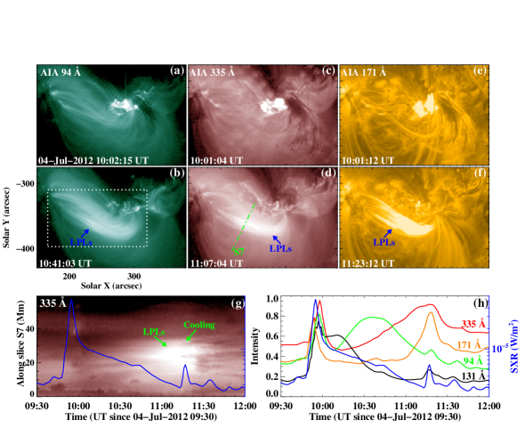
Figure 15: Late phase of the M5.3-class flare. Panels (a)-(f): SDO/AIA 94, 335 and 171 Å images showing the brightening late-phase loops (LPLs) in different wavelengths. The white box in panel (b) is used to obtain the emission variations as shown in panel (h). “S7” in panel (d) is used to obtain the time-distance plot shown in panel (g). Panels (g)-(h): time-distance plot along slice “S7” in 335 Å and the EUV emission variations within the white box (panel (a)) showing the late phase of the flare. Blue curves are the GOES SXR 1-8 Å flux variation of the flare.

One selected event of “type II” flares is the M5.3-class flare occurring in AR 11515 on 2012 July 04. The GOES soft X-ray 1-8 Å flux showed that the flare initiated at 09:47 UT and reached its peak at 09:55 UT (Figures 15(g)-(h)). The SDO/HMI LOS magnetograms showed that the photospheric magnetic field at the flaring region has a tripolar structure in which the negative-polarity patch N1 emerged between positive-polarity sunspot P1 and positive-polarity patch P2 (Figure 12). The emergence of N1 started almost from the beginning of July 03, and simultaneously N1 and P2 exhibited the shearing motion in opposite directions (red and blue arrows in Figures 12(a)-(c)). More significantly, the positive-polarity sunspot P1 showed a converging motion towards the PIL between P1 and N1 (orange arrows in panels (a)-(c)). Along the converging direction (“S5” in panel (a)), we obtained a stack plot based on HMI LOS magnetograms and found that the converging speed of P1 towards the south was about 0.1 km s^-1 (panel (e)). As seen from the 304 Å image, a filament was present along the PIL between P1 and N1 (panel (d)), which erupted later on and generated the M5.3-class flare. The filament had a “reverse S” shape and seemed to be composed of multiple twisted fine structures.

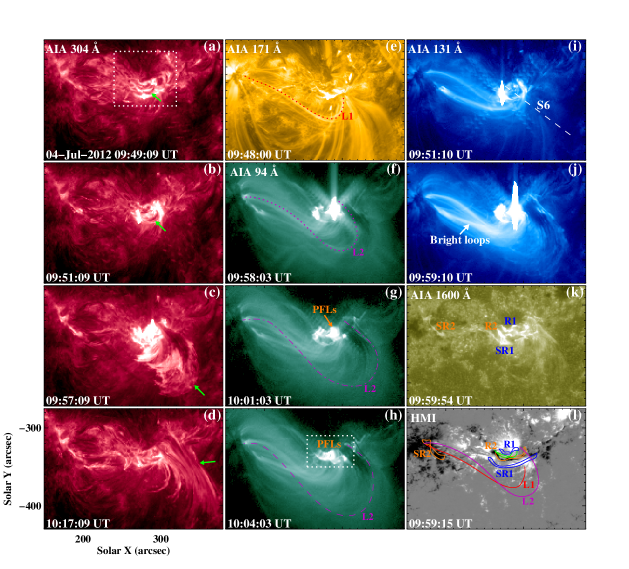
Figure 13: SDO/AIA multi-wavelengths (E)UV images and SDO/HMI LOS magnetogram showing the evolution of the M5.3-class flare on 2012 July 04. Green arrows in panels (a)-(d) point to the erupting filament involved in the event. White rectangles in panels (a) and (h) respectively denote the FOVs of Figures 12(a)-(d) and 14(a)-(c). Red and purple curves in panels (e)-(h) outline two large-scale loop bundles L1 and L2 overlying the flaring region. PFLs in panels (g)-(h) are post-flare loops underlying the eruptive filament in 94 Å. Dashed line “S6” (panel (i)) represents the location used to obtain the stack plot shown in Figures 14(d)-(e). R1 and R2 are two main ribbons, and SR1 and SR2 are two secondary ribbons. The pre-eruption filament (green lines), four flare ribbons (blue and orange contours) and loop bundles (red and purple lines) are plotted over the LOS magnetogram in panel (l). The animation of this figure includes AIA 171, 304, 94 and 131 Å images from 09:30 UT to 11:00 UT. The video duration is 22 s.

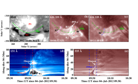
Figure 14: Appearance of post-flare loops (PFLs) and kinematic evolution of the erupting filament. Panels (a)-(c): SDO/HMI LOS magnetogram and SDO/AIA 335 Å images showing the average orientation of the PIL (green curves) of the flaring region and the approximately potential PFLs. P1 and N1 in panel (a) are two magnetic structures where two main ribbons R1 and R2 are located. Purple, red and blue curves in panels (b)-(c) outline three PFLs and their inclination angles with respect to PIL are also shown. Panels (d)-(e): time-distance plots along slice “S6” (Figure 13(i)) in 131 and 335 Å displaying the kinematic evolution of the erupting filament. Two dashed lines respectively denote the start and peak times of the flare.

The 304 Å observations showed that the southwest part of the filament started to rise up slowly from about 09:45 UT and the remanent part was still stable (Figure 13(a)). The ascent of the filament was associated with the EUV brightenings near its two ends (Figure 13(b)). To study the kinematics of the filament in detail, we take a slice along the eruption direction of the filament (“S6” in Figure 13(i)). Figures 14(d)-(e) show the stack plots of the slice in 131 and 335 Å passbands. The evolution of the filament exhibited a slow rise phase and a rapid-acceleration phase. The initial speed of the filament was $\sim$10 km s^-1 during the slow rising process at about 09:45-09:49 UT (Figure 14(d)). The flare was initiated at 09:47 UT, about 2 min later than the slow rise of the filament. Almost from 09:50 UT, the erupting velocity increased rapidly and reached $\sim$100 km s^-1. The 335 Å stack plot shows a larger velocity of $\sim$150 km s^-1 in the impulsive acceleration phase (Figure 14(e)). Later on, the velocity of the filament started to decrease. Finally the filament material drained back along its west leg to the solar surface (Figures 13(c)-(d) and 14(d)-(e)), and the eruption became failed (Ji et al. 2003). As seen from the 171 and 94 Å images, large-scale EUV loops were present over the flaring region (L1 and L2 in Figures 13(e)-(h)). Associated with the eruption of the filament, these large-scale EUV loops were disturbed and pushed outward. Taking L2 for example, its projected height increased by about 24 Mm in 6 min. The flare consisted of two main ribbons (R1 and R2 in Figure 13(k)) and two weakly-brightened secondary ribbons (SR1 and SR2).

Two main ribbons R1 and R2 do not exhibit discernable separation motion perpendicular to the PIL, probably due to the block effect of the strong magnetic field in the sunspot. We also do not see ribbon elongations along the PIL, implying the almost simultaneous magnetic reconnections along the PIL. The pre-eruption filament, four flare ribbons and large-scale loop bundles are plotted over the LOS magnetogram (Figure 13(l)) to analyze their magnetic connectivity. It showed that the filament was located between two main ribbons R1 and R2, implying that the main reconnection process occurs underlying the eruptive filament. R1 and R2 respectively anchored in the converging positive-polarity sunspot P1 and the shearing negative-polarity patch N1 (Figures 12 and 13(l)). Large-scale loop bundle L1 connected two secondary ribbons SR1 and SR2, indicative of their conjugated property. SR1 was located at the southernmost shearing positive-polarity patch P2 and SR2 at the remote negative-polarity sunspot (Figures 12 and 13(l)). Loop bundle L2 was seen to connect the positive and negative sunspots of the AR, which probably constrained the eruption of the filament.

Starting from about 10:00 UT, PFLs appeared underlying the eruptive filament due to the cooling of reconnected loops (Figures 13(g)-(h) and 14(b)-(c)). These PFLs seemed to be quasi-parallel with each other, connecting two main ribbons R1 and R2. As seen from Figure 14(a), the PIL between ribbons R1 and R2 is strongly curved encircling the positive-polarity sunspot. To evaluate the non-potentiality of the PFLs, we measured the inclination angles $\theta$ of PFLs with respect to the PIL (Figures 14(b)-(c)). The $\theta$ value is about 80^∘-86^∘, implying that the PFLs are approximately perpendicular to the PIL and nearly potential fields.

In the decay phase of the flare, the central flare loops gradually faded away, however, another set of longer loops connecting the central flaring region with the remote ribbon started to brighten up (Figures 15(a)-(b)). These brightening loops initially appeared in the high-temperature passbands such as 131 and 94 Å (Figures 13(i)-(j) and 15(a)-(b)), then became visible sequentially in cooler AIA passbands such as 335 (about 2.5 MK) and 171 Å (about 0.6 MK; Figures 15(c)-(f)). These loops are morphologically similar in different passbands, implying that they are the same structures. We cut a slice of the AIA 335 Å images (“S7” in Figure 15(d)) and plotted its time evolution in Figure 15(g). It showed that these longer brightening loops were formed at about 10:45 UT in 335 Å, with a time delay of 50 min after the flare peak. Thus the long brightening loops are identified as late-phase loops (Woods et al. 2011; Liu et al. 2013). About 60 min later, the late-phase loops (LPLs) in 335 Å started to cool down at 11:45 UT. The EUV emissions summed over the cutout of the AR (white rectangle in panel (b)) in different passbands are shown in Figure 15(h). All the EUV emission variations in different passbands exhibit a main phase and a late phase. The emission variations in all temperatures reach their peaks at almost the same time in the main phase, however there are larger time lags between the peaks of the late phase in different temperatures. In 94 Å, the peak flux of the late phase is almost the same as the main phase and the time lag between the two peaks is about 40 min. The time differences between the late phase peaks and the main phase peaks in 335 and 171 Å are 80 and 85 min, respectively.

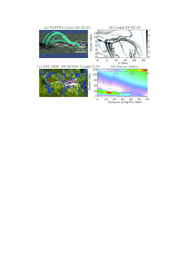
Figure 16: Magnetic field structure and distributions of QSL and decay index. Panel (a): side view of the 3D magnetic topology of the pre-explosion AR at about 09:22 UT on 2012 July 04 resulting from the NLFFF extrapolation. Pink lines are the flux rope (FR) field lines, and cyan lines correspond to the overlying strapping fields. The yellow bar marks the position and extent of the vertical plane where panel (b) is obtained. Panel (b): Q distribution in a vertical plane across the pre-eruptive FR. Q1 is the FR-related QSL and Q2 is the dome-shaped QSL encircling Q1. Panel (c): overlay between the flare ribbons (underlying 1600 Å image) and the QSL map (blue curves). All regions with Q_thresh$>$10^3.5 are shown in this panel. The PIL between two main ribbons R1 and R2 is extracted from the bottom boundary of the extrapolated NLFFFs and marked by the red curve. The “$\times$” symbol shows the starting point of the PIL. Panel (d): distribution of the decay index above the PIL (red curve in panel (c)) prior to the flare onset. The white lines mark the positions where decay index n reaches the critical value of 1.5.

The topology of the 3D magnetic field reveals the existence of a flux rope (FR) and the overlying constraining fields (Figure 16(a)). FR is moderately twisted with an average twist number of 2.0, and bears a good resemblance to the observed filament (Figures 12 and 13). The overlying cyan fields connect the flaring region with remote brightenings, corresponding to the identified large-scale loop bundles L1 and L2 in Figure 13. As seen from the distribution of the Q factor (Figure 16(b)) in a vertical plane across the pre-eruptive FR axis (yellow bar in Figure 16(a)), a QSL structure (Q1) of upside-down teardrop shape at the boundary of the FR and a larger dome-shaped QSL (Q2) encircling Q1 are present. In panel (c), we show the matches between the QSLs and the flare ribbons. It is seen that the flare ribbons are well matched with the two QSLs (Q1 and Q2). At the locations of two strongly curved main ribbons R1 and R2, the intersections of Q1 with the lower boundary are present and display the similar shapes with ribbons R1 and R2. This implies that magnetic reconnection probably occurs at the FR-related Q1 underlying the FR and results in the formation of main ribbons R1 and R2 (Janvier et al. 2014; Jiang et al. 2018; Liu et al. 2018a), which is consistent with the CSHKP flare model. The majority of secondary ribbon SR1 is well matched by the southern footpoints of the dome-shaped Q2. We note that the west hook of SR1 is poorly matched, probably due to the higher complexity of magnetic fields at this location. The remote secondary ribbon SR2 shows a good correspondence with the remote footpoints of Q2 (eastern ends of cyan lines in panel (a)), indicative of the occurrence of secondary magnetic reconnection along the large-scale Q2.

In Figure 16(d), we display the distribution of the decay index n above the PIL prior to the flare onset. It is seen that the decay index n shows an unusual distribution. Above the eastern half of the PIL (30-60 Mm along the PIL), n reaches 1.5 at varying heights, which are all above 90 Mm, suggesting the presence of strong confinement at this region. Above the western half of the PIL (0-30 Mm along the PIL), n reaches 1.5 at a height around 15 Mm, keeping larger than 1.5 until 40 Mm, then drops below 1.5 in a large range of height (from 40 Mm to a height larger than 150 Mm), though n is increasing in this height range. This kind of distribution is called a “saddle-like” profile, which has been studied (Guo et al. 2010; Wang et al. 2017; Liu et al. 2018b), and is usually associated with failed eruption. The “saddle-like” profile exhibits a local torus-stable (n$<$1.5) region enclosed by two torus-unstable domains. Eruptions occurring in a region having “saddle-like” decay index distribution may be slowed down in the highly located torus-stable region if the initial disturbance is not large enough, thus fails to erupt out into the interplanetary space. In our case, the eruption of the filament occurred at the western part of the filament (see Figure 13), above which n had a “saddle-like” distribution, having an apparent rising velocity around 150 km s^-1 (Figure 14). The eruption may happen when the flux rope supporting the filament enters the local torus-unstable region between 15-40 Mm. It keeps rising up and then enters the torus-stable region. This region provides strong confinement again. With a small initial velocity, the flux rope has no enough disturbance to erupt out and is slowed down by the slow decaying, strong strapping fields in the torus-stable region. The particular distribution of n, along with the clear signature of a failed eruption of a filament, suggests that the strong confinement above the filament plays the major role in confining the eruption in this case.

4 Discussion

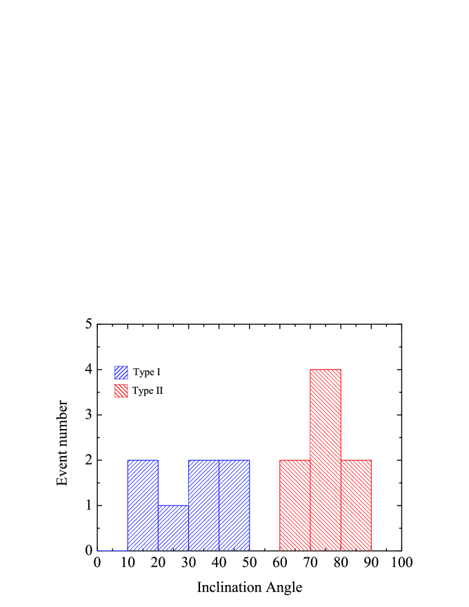
Figure 17: Histogram of measured inclination angle of PFLs for the 15 confined flares. Blue/red represents “type I”/“type II” flares. The bin size in the histogram is $10^{\circ}$.

The two types of flares display different flaring structures and dynamic evolution. We estimated the inclination angles $\theta$ of PFLs with respect to the PIL for 15 flares (PFLs in 3 circular-ribbon flares are too compact and thus are not measured in Table 1) and displayed the histogram for the two types of flares in Figure 17. It shows that the $\theta$ for “type I” is in the range from $10^{\circ}$ to $50^{\circ}$. The $\theta$ for “type II” is evidently higher than “type I”, in the range of $60^{\circ}$- $90^{\circ}$. The difference of the $\theta$ value for the two types of flares is probably caused by the different magnetic environments where reconnection occurs. For “type I” flares, slipping reconnection occurs between two sets of magnetic systems and results in the interchange of their magnetic connectivities. The mutual orientation between two reconnecting systems is less favorable for reconnection, and thus the reconnection is limited and the new reconnected magnetic field is still strongly sheared (Galsgaard et al. 2007; Zuccarello et al. 2017). For “type II” flares, magnetic reconnection occurs in anti-parallel magnetic fields underlying the erupting flux rope or at the 3D null-point in the fan-spine topology, which is the effective reconnection process leading to the flux rope erupiton (Archontis & Török 2008; Leake et al. 2013, 2014). In this situation, a large majority of free magnetic energy is released and the newly formed PFLs generally relax fully to a quasi-potential state.

In order to estimate the magnetic field gradient in the environment of the filaments, we computed the distribution of the decay index n above the PIL. For the first flare on 2011 March 09, the decay index distribution has a modest critical height around 45 Mm (Figure 6). While for the event occurring on 2014 October 26, the distribution has a critical height above 90 Mm (Figure 11). The former is a modest height with which both confined and eruptive flares may occur (e.g., Liu et al. 2016a). The latter seems to indicate a strong confinement overlying the filament. However, the magnetic reconnections during the two “type I” flares occur in these strapping fields overlying the filaments (MS1 and MS2 in Figures 6(a) and 11(a)), so it is difficult to distinguish the overlying fields as reconnecting fields or confining fields. In both events, the filaments are stable and do not show any eruption signatures. Thus the confinement of the overlying strapping fields, no matter it is large or small, would not play a significant role in the eruptiveness of the flares. We suggest that the analysis of the decay index in complex “type I” flares does not provide a useful clue for the class of eruption (Zuccarello et al. 2017).

For the “type II” flare on 2012 July 04, the decay index distribution has a “saddle-like” profile at the western part above the filament (Figure 16), having a local torus-unstable region within 15-40 Mm, which is enclosed by two torus-stable regions. The filament experienced a failed eruption at the western part of the PIL with a relatively slow initial velocity around 150 km s^-1 (Figures 13-14). With this small initial disturbance, the flux rope supporting the filament may be slowed down in the higher located torus-stable region, thus fails to erupt out. Unlike “type I” confined flares, this “type II” event has clear failed eruption signatures, and its post-flare loops have weakly sheared configuration, suggesting that most helicity of the erupting system is released during the eruption. Thus, a flux rope must have erupted at first, though finally being stopped in the higher corona. The strong confinement of the strapping magnetic fields should have played a significant role in confining the eruption associated with this kind of standard confined flares.

All the “type I” flares exhibit the elongation motion parallel to the PIL at speeds of a few tens of km s^-1 (Table 1). The elongation motion of flare ribbons is not present in a 2D framework, however, it can be explained by the 3D reconnection along the QSLs (Priest & Démoulin 1995; Masson et al. 2012). High-resolution observations of the IRIS displayed the bi-directional slipping motion of ribbon substructures (Figure 8). We suggest that the slipping substructures along two directions respectively correspond to the footpoints of two magnetic systems (MS1 and MS2 in Figure 11). The continuous slipping magnetic reconnection between the two magnetic systems results in the exchange of their connectivities and the tangential movement of reconnecting field lines one to each other. Flare loops in this kind of flares also displayed the apparent slipping motions along the ribbons. In the first event, the acceleration process of the slipping motion during the flare is first presented (Figure 3). The slippage of flare loops exhibits two kinematic phases: a slow slipping phase and a fast slipping phase. The simulation results of Janvier et al. (2013) showed that the slipping speed of field lines would increase as the expansion of the torus-unstable flux rope resulted in the evolution of QSLs toward separatrices. The acceleration of the slippage in our observations implies that the QSLs are displaced devoid of any flux rope eruption. All these observations of flare loops or ribbon motions during “type I” confined flares provide the evidence for slipping magnetic reconnections between different sets of magnetic systems. The constant flux emergence and shearing motion (Figure 1) probably help to accumulate the current at the interface between the two systems (Krall et al. 1982; Yan et al. 2018). Magnetic reconnections could occur within the current layer in the vicinity of QSLs, similar to the simulations of Aulanier et al. (2005). The slipping reconnection causes no significant topological change and thus the equilibrium of the entire system is not destabilized. The flares finally develop into confined events due to the lack of any erupting magnetic structures such as magnetic flux ropes and sheared magnetic loop bundles. The scenario of “type I” confined flares is similar to the “unorthodox” and “atypical” flares in previous case studies (Liu et al. 2014; Dalmasse et al. 2015; Joshi et al. 2019), which are both inconsistent with the classical flare models.

“Type II” confined flares are accompanied by the flux rope eruption, that becomes failed due to the presence of strong strapping fields overlying the flaring region. They can be described by the classical flare models. The two-ribbon “type II” flares are consistent with the CSHKP model (Shibata & Magara 2011) and its extension in 3D (Aulanier et al. 2012; Janvier et al. 2014). The circular-ribbon “type II” flares have a fan-spine topology and the null-point reconnections lead to the occurrence of the flares (Lau & Finn 1990; Priest & Titov 1996; Liu et al. 2011). The early dynamic evolution of the “type II” flare is similar to eruptive flares, differently, the material motion of the filament is hindered and its trajectory is changed while encountering with the ambient background fields in the gradual phase of the flare. This kind of confined flares has been extensively studied and the strength of the overlying field is thought to be an important factor determining whether a flare is confined (Cheng et al. 2011; Nindos et al. 2012; Liu et al. 2016a; Amari et al. 2018). In the event on 2012 July 04, the formations of secondary flare ribbons and late-phase flare loops (Figures 13 and 15) both suggest that the large-scale constraining fields overlying the erupting flux rope are partially reconnected (Sun et al. 2013; Dai & Ding 2018). However, the remaining constraining fields that are not reconnecting still hold a high flux ratio compared to the flux rope, hence inhibit the eruption of the flux rope.

5 Conclusion

In this study, we selected 18 confined flares (GOES class $\geq$M5.0 and $\leq$$45^{\circ}$ from disk center) that occurred between 2011 January and 2017 December, i.e., 7 yr from the activity minimum of solar cycle 24. According to their different dynamic properties and magnetic configurations, we first divide the confined flares into two types. For “type I” confined flares, the magnetic configuration is very complex with two or more QSLs overlying the core magnetic structure, and multiple slipping reconnections along these QSLs trigger the occurrence of the flare. Eventually, the slipping magnetic reconnections do not cause any eruption of magnetic structures and the entire magnetic system still remains stabilized. “Type II” confined flare has the magnetic configuration consistent with the classical flare models, but strong strapping fields are present over the flaring region in the high atmosphere. Based on the classification criteria, 7 flares of 18 ($\sim$39 %) belong to “type I” and 11 ($\sim$61 %) are “type II” confined flares.

The complexity of the magnetic fields involved in “type I” flares is shown in several aspects. The pre-flare loops and PFLs are both composed of two or more sets of magnetic systems. PFLs have a stronger non-potentiality, with the inclination angle $\theta$ in the range of 10^∘-50^∘. All the “type I” flares exhibit the ribbon elongations parallel to the PIL at speeds of several tens of km s^-1. All these observations indicate the 3D nature of magnetic reconnection in solar flares. We suggest that magnetic reconnection between different magnetic systems results in the flare occurrence. However, the reconnection is probably limited and has a low efficiency for the mutual orientation between two systems is less favorable for reconnection. Thus the equilibrium of the entire system is not destabilized and the flare finally develops into a confined event.

The two types of confined flares show distinct properties in several aspects. The complex PFLs in “type I” flares are composed of two or more sets of magnetic connectivities overlying the non-eruptive filament and are strongly sheared. However, the PFLs in “type II” flares are formed underlying the erupting magnetic structure. They are approximately parallel with each other and have a weak non-potentiality. Moreover, all the “type I” flares exhibit the ribbon elongations along the PIL at apparent speeds of several tens of km s^-1, suggestive of the occurrence of slipping magnetic reconnections along the QSLs. Only 3 of 10 “type II” flares display the ribbon elongations. This implies that unlike “type I” flares the QSL reconnection is probably not dominant in “type II” flares, and in most “type II” flares magnetic reconnection is almost simultaneous along the current sheet, consistent with the CSHKP model. The filament at the flaring region plays different roles in these two types of confined events. The filament in “type I” seems not to be affected by the flare and is not associated with any eruption process. In “type II”, the filament becomes unstable due to the loss of equilibrium or suffering MHD instabilities, and the rise of the filament causes the subsequent reconnection and the occurrence of the flare.

Overall, our results suggest that there are two types of confined flares that are triggered by different physical mechanisms. To our knowledge, “type II” confined flares have been extensively studied in the literature and the main reason for the confinement has been well understood. However, “type I” confined flares have been rarely analyzed due to their complexity. Our study shows that “type I” accounts for more than one third of all the large confined flares, which should not be neglected in further studies.

Table 1: Event list

Event	Date	Time	GOES	AR	Filament	Separation	Elongation	Angle	Type I/II
No.			class			(km s-1)	(km s-1)	(degree)
1	20110309	23:23	X1.5	11166	S	No	33$\pm$3	48$\pm$2	I
2	20110730	02:09	M9.3	11261	E	5$\pm$1	11$\pm$2	74$\pm$2	II
3	20120510	04:18	M5.7	11476	E	No	No	-	II
4	20120704	09:55	M5.3	11515	E	No	No	83$\pm$2	II
5	20120705	11:44	M6.1	11515	E	No	No	82$\pm$2	II
6	20131101	19:53	M6.3	11884	E	No	15$\pm$3	64$\pm$2	II
7	20140107	10:13	M7.2	11944	E	No	No	-	II
8	20140204	04:00	M5.2	11967	E	No	No	71$\pm$2	II
9	20141022	01:59	M8.7	12192	S	12$\pm$2	45$\pm$5	34$\pm$2	I
10	20141022	14:28	X1.6	12192	S	No	16$\pm$4	45$\pm$2	I
11	20141024	21:40	X3.1	12192	S	15$\pm$2	23$\pm$4	25$\pm$2	I
12	20141025	17:08	X1.0	12192	S	10$\pm$1	12$\pm$2	20$\pm$2	I
13	20141026	10:53	X2.0	12192	S	21$\pm$2	20$\pm$3	18$\pm$2	I
14	20141027	00:34	M7.1	12192	A	No	11$\pm$3	37$\pm$2	I
15	20141204	18:25	M6.1	12222	E	12$\pm$3	No	79$\pm$2	II
16	20150824	07:33	M5.6	12403	E	-	-	-	II
17	20150928	14:58	M7.6	12422	E	No	No	67$\pm$2	II
18	20170906	09:10	X2.2	12673	E	8$\pm$1	10$\pm$2	73$\pm$2	II

• Notes.

• Flare peak time.

• The filament dynamics in the flaring region: “S”, “E” and “A” respectively means stable, eruptive and activated.

• The separation motion of flare ribbons perpendicular to the PIL. The velocity is obtained by the linear fitting to the stack plot along a slice perpendicular to the PIL. We assumed an error of two pixels (1$\arcsec$.2) in the location measurement and the uncertainty in the speed was thus estimated according to different durations of the separation motions.

• The elongation motion of flare ribbons along the PIL. The velocity is obtained by the linear fitting to the stack plot along a slice along the ribbon. The error estimation is similar to the separation motion.

• The inclination angle $\theta$ of PFLs with respect to the PIL. $\theta$ is the average value by measuring different PFLs that can be clearly discerned. If there are two or more sets of PFLs, $\theta$ corresponds to the most strongly sheared set of loops. The PIL information used in this study is from the LOS photospheric magnetograms from the SDO/HMI.

References

- (1) Amari, T., Canou, A., Aly, J.-J., Delyon, F., & Alauzet, F. 2018, Nature, 554, 211
- (2) Archontis, V., & Török, T. 2008, A&A, 492, L35
- (3) Aulanier, G., Janvier, M., & Schmieder, B. 2012, A&A, 543, A110
- (4) Aulanier, G., Pariat, E., & Démoulin, P. 2005, A&A, 444, 961
- (5) Aulanier, G., Pariat, E., Démoulin, P., & DeVore, C. R. 2006, Sol. Phys., 238, 347
- (6) Bateman, G. 1978, MHD Instabilities (Cambridge, MA: MIT Press)
- (7) Baumgartner, C., Thalmann, J. K., & Veronig, A. M. 2018, ApJ, 853, 105
- (8) Bobra, M. G., Sun, X., Hoeksema, J. T., et al. 2014, Sol. Phys., 289, 3549
- (9) Carmichael, H. 1964, NASA Special Publication, 50, 451
- (10) Chandra, R., Schmieder, B., Mandrini, C. H., et al. 2011, Sol. Phys., 269, 83
- (11) Chen, H., Zhang, J., Ma, S., et al. 2015, ApJ, 808, L24
- (12) Cheng, X., Zhang, J., Ding, M. D., Guo, Y., & Su, J. T. 2011, ApJ, 732, 87
- (13) Dai, Y., & Ding, M. 2018, ApJ, 857, 99
- (14) Dalmasse, K., Chandra, R., Schmieder, B., & Aulanier, G. 2015, A&A, 574, A37
- (15) Démoulin, P., Priest, E. R., & Lonie, D. P. 1996, J. Geophys. Res., 101, 7631
- (16) De Pontieu, B., Title, A. M., Lemen, J. R., et al. 2014, Sol. Phys., 289, 2733
- (17) Dudík, J., Janvier, M., Aulanier, G., et al. 2014, ApJ, 784, 144
- (18) Dudík, J., Polito, V., Janvier, M., et al. 2016, ApJ, 823, 41
- (19) Falconer, D. A., Moore, R. L., & Gary, G. A. 2002, ApJ, 569, 1016
- (20) Falconer, D. A., Moore, R. L., & Gary, G. A. 2006, ApJ, 644, 1258
- (21) Galsgaard, K., Archontis, V., Moreno-Insertis, F., & Hood, A. W. 2007, ApJ, 666, 516
- (22) Gopalswamy, N., Yashiro, S., Michalek, G., et al. 2009, Earth Moon and Planets, 104, 295
- (23) Gosling, J. T., McComas, D. J., Phillips, J. L., & Bame, S. J. 1991, J. Geophys. Res., 96, 7831
- (24) Gou, T., Liu, R., Wang, Y., et al. 2016, ApJ, 821, L28
- (25) Green, L. M., Matthews, S. A., van Driel-Gesztelyi, L., Harra, L. K., & Culhane, J. L. 2002, Sol. Phys., 205, 325
- (26) Guo, Y., Ding, M. D., Schmieder, B., et al. 2010, ApJ, 725, L38
- (27) Hermans, L. M., & Martin, S. F. 1986, BAAS, 18, 991
- (28) Hirayama, T. 1974, Sol. Phys., 34, 323
- (29) Hong, J., Jiang, Y., Yang, J., Li, H., & Xu, Z. 2017, ApJ, 835, 35
- (30) Hou, Y., Zhang, J., Li, T., Yang, S. H., & Li, X. H. 2018, A&A, 619, A100
- (31) Howard, R. A., Moses, J. D., Vourlidas, A., et al. 2008, Space Sci. Rev., 136, 67
- (32) Inoue, S., Hayashi, K., & Kusano, K. 2016, ApJ, 818, 168
- (33) Janvier, M., Aulanier, G., Bommier, V., et al. 2014, ApJ, 788, 60
- (34) Janvier, M., Aulanier, G., Pariat, E., & Démoulin, P. 2013, A&A, 555, A77
- (35) Ji, H., Wang, H., Schmahl, E. J., Moon, Y.-J., & Jiang, Y. 2003, ApJ, 595, L135
- (36) Jiang, C., Wu, S. T., Yurchyshyn, V., et al. 2016, ApJ, 828, 62
- (37) Jiang, C., Zou, P., Feng, X., et al. 2018, ApJ, 869, 13
- (38) Jing, J., Liu, C., Lee, J., et al. 2018, ApJ, 864, 138
- (39) Jing, J., Liu, R., Cheung, M. C. M., et al. 2017, ApJ, 842, L18
- (40) Joshi, N. C., Zhu, X., Schmieder, B., et al. 2019, ApJ, 871, 165
- (41) Kaiser, M. L., Kucera, T. A., Davila, J. M., et al. 2008, Space Sci. Rev., 136, 5
- (42) Kliem, B., & Török, T. 2006, Physical Review Letters, 96, 255002
- (43) Kopp, R. A., & Pneuman, G. W. 1976, Sol. Phys., 50, 85
- (44) Krall, K. R., Smith, J. B., Jr., Hagyard, M. J., West, E. A., & Cummings, N. P. 1982, Sol. Phys., 79, 59
- (45) Krucker, S., Hurford, G. J., & Lin, R. P. 2003, ApJ, 595, L103
- (46) Lau, Y.-T., & Finn, J. M. 1990, ApJ, 350, 672
- (47) Lee, J., & Gary, D. E. 2008, ApJ, 685, L87
- (48) Lemen, J. R., Title, A. M., Akin, D. J., et al. 2012, Sol. Phys., 275, 17
- (49) Li, H., Liu, Y., Liu, J., Elmhamdi, A., & Kordi, A.-S. 2018a, PASP, 130, 124401
- (50) Li, T., Hou, Y., Yang, S., & Zhang, J. 2018b, ApJ, 869, 172
- (51) Li, T., Yang, K., Hou, Y., & Zhang, J. 2016, ApJ, 830, 152
- (52) Li, T., & Zhang, J. 2014, ApJ, 791, L13
- (53) Li, T., & Zhang, J. 2015, ApJ, 804, L8
- (54) Liu, K., Zhang, J., Wang, Y., & Cheng, X. 2013, ApJ, 768, 150
- (55) Liu, L., Cheng, X., Wang, Y., et al. 2018a, ApJ, 867, L5
- (56) Liu, L., Wang, Y., Wang, J., et al. 2016a, ApJ, 826, 119
- (57) Liu, L., Wang, Y., Zhou, Z., et al. 2018b, ApJ, 858, 121
- (58) Liu, R., Kliem, B., Titov, V. S., et al. 2016b, ApJ, 818, 148
- (59) Liu, R., Titov, V. S., Gou, T., et al. 2014, ApJ, 790, 8
- (60) Liu, W., Berger, T. E., Title, A. M., Tarbell, T. D., & Low, B. C. 2011, ApJ, 728, 103
- (61) Masson, S., Aulanier, G., Pariat, E., & Klein, K.-L. 2012, Sol. Phys., 276, 199
- (62) Masson, S., Pariat, E., Aulanier, G., & Schrijver, C. J. 2009, ApJ, 700, 559
- (63) Nindos, A., & Andrews, M. D. 2004, ApJ, 616, L175
- (64) Nindos, A., Patsourakos, S., & Wiegelmann, T. 2012, ApJ, 748, L6
- (65) O’Dwyer, B., Del Zanna, G., Mason, H. E., Weber, M. A., & Tripathi, D. 2010, A&A, 521, A21
- (66) Park, S.-H., Guerra, J. A., Gallagher, P. T., Georgoulis, M. K., & Bloomfield, D. S. 2018, Sol. Phys., 293, 114
- (67) Pesnell, W. D., Thompson, B. J., & Chamberlin, P. C. 2012, Sol. Phys., 275, 3
- (68) Priest, E. R., & Démoulin, P. 1995, J. Geophys. Res., 100, 23443
- (69) Priest, E. R., & Forbes, T. G. 2002, A&A Rev., 10, 313
- (70) Priest, E. R., & Titov, V. S. 1996, Philosophical Transactions of the Royal Society of London Series A, 354, 2951
- (71) Qiu, J., Longcope, D. W., Cassak, P. A., & Priest, E. R. 2017, ApJ, 838, 17
- (72) Sarkar, R., & Srivastava, N. 2018, Sol. Phys., 293, 16
- (73) Savcheva, A., Pariat, E., McKillop, S., et al. 2015, ApJ, 810, 9
- (74) Scherrer, P. H., Schou, J., Bush, R. I., et al. 2012, Sol. Phys., 275, 207
- (75) Schmieder, B., Aulanier, G., Demoulin, P., et al. 1997, A&A, 325, 1213
- (76) Shen, Y.-D., Liu, Y., & Liu, R. 2011, Research in Astronomy and Astrophysics, 11, 594
- (77) Shibata, K., & Magara, T. 2011, Living Reviews in Solar Physics, 8, 6
- (78) Sturrock, P. A. 1966, Nature, 211, 695
- (79) Su, Y., Golub, L., & Van Ballegooijen, A. A. 2007, ApJ, 655, 606
- (80) Su, Y. N., Golub, L., van Ballegooijen, A. A., & Gros, M. 2006, Sol. Phys., 236, 325
- (81) Sun, X., Bobra, M. G., Hoeksema, J. T., et al. 2015, ApJ, 804, L28
- (82) Sun, X., Hoeksema, J. T., Liu, Y., et al. 2013, ApJ, 778, 139
- (83) Svestka, Z., & Cliver, E. W. 1992, in IAU Colloq. 133, Eruptive Solar Flares, Vol. 399, ed. Z. Svestka, B. V. Jackson, & M. E. Machado (New York: Springer), 1
- (84) Thalmann, J. K., Su, Y., Temmer, M., & Veronig, A. M. 2015, ApJ, 801, L23
- (85) Titov, V. S., Hornig, G., & Démoulin, P. 2002, Journal of Geophysical Research (Space Physics), 107, 1164
- (86) Tziotziou, K., Georgoulis, M. K., & Raouafi, N.-E. 2012, ApJ, 759, L4
- (87) Wang, D., Liu, R., Wang, Y., et al. 2017, ApJ, 843, L9
- (88) Wang, Y., & Zhang, J. 2007, ApJ, 665, 1428
- (89) Wheatland, M. S., Sturrock, P. A., & Roumeliotis, G. 2000, ApJ, 540, 1150
- (90) Wiegelmann, T. 2004, Sol. Phys., 219, 87
- (91) Wiegelmann, T., Inhester, B., & Sakurai, T. 2006, Sol. Phys., 233, 215
- (92) Woods, T. N., Hock, R., Eparvier, F., et al. 2011, ApJ, 739, 59
- (93) Yan, X. L., Wang, J. C., Pan, G. M., et al. 2018, ApJ, 856, 79
- (94) Yang, K., Guo, Y., & Ding, M. D. 2015, ApJ, 806, 171
- (95) Yang, S., Zhang, J., & Xiang, Y. 2014, ApJ, 793, L28
- (96) Zhang, J., Li, T., & Chen, H. 2017, ApJ, 845, 54
- (97) Zhao, J., Li, H., Pariat, E., et al. 2014, ApJ, 787, 88
- (98) Zheng, R., Chen, Y., & Wang, B. 2016, ApJ, 823, 136
- (99) Zuccarello, F. P., Aulanier, G., & Gilchrist, S. A. 2015, ApJ, 814, 126
- (100) Zuccarello, F. P., Chandra, R., Schmieder, B., Aulanier, G., & Joshi, R. 2017, A&A, 601, A26