Restoring Images with Unknown Degradation Factors
by Recurrent Use of a Multi-branch Network

Abstract

The employment of convolutional neural networks has achieved unprecedented performance in the task of image restoration for a variety of degradation factors. However, high-performance networks have been specifically designed for a single degradation factor. In this paper, we tackle a harder problem, restoring a clean image from its degraded version with an unknown degradation factor, subject to the condition that it is one of the known factors. Toward this end, we design a network having multiple pairs of input and output branches and use it in a recurrent fashion such that a different branch pair is used at each of the recurrent paths. We reinforce the shared part of the network with improved components so that it can handle different degradation factors. We also propose a two-step training method for the network, which consists of multi-task learning and fine-tuning. The experimental results show that the proposed network yields at least comparable or sometimes even better performance on four degradation factors as compared with the best dedicated network for each of the four. We also test it on a further harder task where the input image contains multiple degradation factors that are mixed with unknown mixture ratios, showing that it achieves better performance than the previous state-of-the-art method designed for the task.

1 Introduction

The problem of image restoration, i.e., restoring an original, clean image from its degraded version(s), has been studied for a long time in computer vision and image processing. As with other problems of computer vision, deep learning has been applied to this problem, leading to significant improvement of performance. There are many factors causing image degradation, for each of which there are a large number of studies in the past, such as motion/defocus blur [56, 47, 71, 70, 12], several types of noises (e.g., Gaussian, real-world noise, etc.) [13, 9, 69, 68], JPEG compression noise [76, 8, 4, 25], rain streak [38, 28, 10], raindrop [33, 79, 29], haze [23, 45, 2] etc.

Previous studies have treated each of these degradation factors individually and developed “dedicated” methods for each factor. It is also the case with recent studies utilizing deep learning[32, 50, 59, 37, 78, 82]; This means that it needs to be known in advance which factor of degradation needs to be removed from the image. Although this will be fine for photo-editing software, where users specify it, this is insufficient for real-world applications such as self-driving/driver assistance and surveillance.

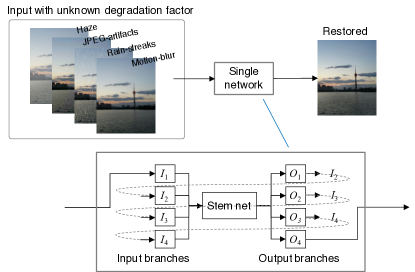
Figure 1: Illustration of the goal and our approach. To restore a clean image from an input with unknown degradation factor, we use a network with multiple input and output branches. Receiving an input image from $I_{1}$, it yields an improved image in terms of a single degradation factor from $O_{1}$. It is then fed to $I_{2}$ and improved in terms of another factor, outputting the improved image from $O_{2}$. This is repeated until $O_{4}$, yielding the final output. Each box inside the bottom large box represents a sub-network.

Thus, it is desirable to enable to deal with input images with unknown degradation factor(s), as shown in the upper row of Fig. 1. It should be noted that a few studies tackled this problem [80, 58]. However, their performances are no so high; they are significantly lower than those of dedicated networks used in the ideal case when they are applied to images having the assumed degradation factor.

How can we restore images with unknown degradation factors to a higher level? We can think of two approaches. One is to build a universal network that can deal with any degradation factors; it is a network equipped with a single input receiving a degraded image and a single output yielding a restored image. However, such a design has difficulty. A very successful approach to image restoration so far is to have a network predict only the difference from the input image to the desired high-quality image [42, 51, 37], as shown in Fig. 2. As seen in the figure, the residual images tend to have considerably different statistical properties for different factors, making it difficult to have a single output deal with them.

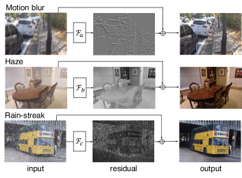
Figure 2: The approach that is currently very successful for image restoration tasks. CNNs $\mathcal{F}^{\prime}s$ are used to predict the difference (or residue) from an input to its ideally restored version (i.e., a clean image). A single network is designed and trained for each task.

The other approach is to cascade multiple networks, each of which is a dedicated network for a single factor. It should perform well if each component network works well on the target factor and also does no harm on the other factors as well as restored clean images. This approach, however, will suffer from a high memory consumption; the total number of parameters in the cascade increases proportionally with the number of factors we consider, leading to excessive memory use in the case of many factors.

In this paper, we consider yet another (the third) approach, which may be considered as an intermediate solution between the above two. We consider a single network with multiple input and output branches, as shown in Fig. 1. Each output branch forms a pair with one of the input branches, which is used for removing a single degradation factor. Then, we recurrently use this network, that is, we feed the output from an output branch back to one of the input branches and repeat this procedure for the number of factors with a different input-output pair at each time. (This may be viewed as a cascading repetition of the same network with each cascading point connected with a different input-output pair.) To train the network, we consider a two-step method; in the first step, we train it in a multi-task learning (MTL) framework, and in the second step, we fine-tune it so that it can be used in a recurrent manner.

This approach resolves the difficulties above with the two approaches. As the network has multiple input and output branches, we can employ the standard formulation of predicting a residual image for each factor. Our training scheme enables us to equip the network with the property that it does not affect the factors other than the target one including clean images.

Although our network has multiple input and output branches, its stem, i.e., the shared main body, is dominant in terms of the number of parameters. To provide it with a sufficient representational power to deal with multiple degradation factors, we propose a new design of a network component built upon the dual residual networks, which was recently proposed by Liu et al. [42]. Although the authors have shown that the base network architecture is effective for various degradation factors, its internal components need to be changed for different degradation factors. We present two improvements to its basic block. One is an improved attention mechanism that utilizes amplitude of spatial derivatives of activation (i.e., $|I^{(c)}_{x}|$ and $|I^{(c)}_{y}|$) to compute attention weights. The other is a new internal design, in which the two operations employed in DuRB-U and -US [42] are fused; we will refer to it as DuRB-M. We show through experiments that these two improvements do contribute to achieving the goal of this study.

2 Related Work

Image Restoration

Image restoration has been studied for a long time. Most of the early studies incorporate models of degraded images along with priors of clean natural images, based on which they formulate and solve an optimization problem. Examples are the studies on motion blur removal [15, 71, 70, 1] and those on haze removal [23, 3, 45]. Recently, CNN-based methods have achieved good performance for all sorts of image restoration tasks [60, 18, 46, 82, 74, 52, 83, 37, 35, 87, 67, 14, 44]. For motion blur removal, Nah et al. [46] proposed a network architecture having modified residual blocks and trained it on a large scale dataset (GoPro Data). Kupyn et al. [32] proposed a GAN [20] -based method, updating the former state-of-the-art. For haze removal, Zhang et al. [82] proposed a GAN-based CNN that jointly estimates multiple unknowns comprising a haze model. Ren et al. [53] proposed a method of weighting several enhanced versions of an input image with the weights predicted by a CNN.

For rain-streak removal, Li et al. proposed a RNN-based method [37] and Li et al. proposed non-locally enhanced dense block (NEDB) [35]. For JPEG-compression noise removal, Galteri et al. [16] proposed a GAN-based method and Zhang et al. [87] proposed a non-local attention mechanism. Finally, Liu et al. recently proposed a network architecture having dual residual connections, updating state-of-the-art performance on most of the above tasks.

Single Net for Multiple Degradation Factors   A more challenging problem is to restore a clean image from an input image with an unknown combination of multiple degradation factors, which were studied in [80, 58]. However, there seems to be a large room for improvement, because the performances of their methods are inferior with large margin to the state-of-the-art method designed for each single factor in the removal performance of that factor. There are studies that train a network on two or more degradation factors that are similar (e.g., deblurring and super-resolution [72, 86]) or closely related with each other (e.g., denoising and deblur/decompression [19, 46] and rain-streak and haze [36]) to improve performance. These methods are specifically designed for a particular set of degradation factors; thus it will be hard to apply them to the removal of a diverse range of factors. There are also studies that train different networks with an identical design on different degradation factors e.g., noise, rain-streak, and super-resolution [31]; or noise, mosaic, JPEG-compression noise, and super-resolution [87]. Our study differs from these in the motivation explained in Sec. 1 and also in that we train the same network on multiple factors.

Use of Recurrent Paths for Image Restoration   A number of studies on image-to-image translation tasks have employed the idea of using the entire or a part of a network in a recurrent fashion for several purposes, such as improved efficiency and accuracy, e.g., image compression [27], saliency detection [48], segmentation [66], and depth estimation [64]. It has been adopted for image restoration tasks on single images [21, 84, 61, 50] as well as videos [40, 55, 75]. For instance, it has been shown [61, 17, 6] that recurrently scaling-up input images for training networks is effective for dynamic scene deblurring. Gao et al. [17] point out that blurring effects vary in magnitude depending on the scale of input images. While sharing all layers to deal with multiple scales often ends up with learning only single-scale features, assigning different layers for different scales [46, 6] is inefficient. Thus, they propose a selective sharing approach to share all layers for multiple scales of input images except the convolutional layers at the beginning and end, and those employed for down/up-scaling. For the rain-streak removal task, it has been known to be an effective strategy to progressively restore a clean image from the input. This strategy is implemented by repeatedly sending the output of a network back to its input and performing forward computation; for this purpose, multiple gating units (e.g. LSTM) is employed [37] or one Conv-LSTM is used at the beginning of the network [51].

Multi-task Learning   It has been well known that multi-task learning (MTL) [7] is effective for deep networks applied to many computer vision tasks; [7, 43, 30, 73, 22, 39] to name a few. To enable MTL to work, there should arguably be some relation among the tasks jointly learned; in other words, there should be overlaps among the representations to be learned inside networks for those tasks. It remains unknown if MTL is effective for diverse image restoration tasks; different degradation factors could be orthogonal with each other. In fact, the aforementioned studies on the restoration from combined degradation factors attempt to deal with different factors by adaptively selecting different networks [80] or different operations [58] depending on the factors existing in the input image.

3 Design of the Proposed Network

As shown in Fig. 1, the proposed network consists of multiple input branches, a stem network, and multiple output branches. We first describe the design of the stem network, and then present the design of output branches and finally input branches.

3.1 Design of the Stem Network

The stem network, which occupies the dominant portion in the entire network in terms of the number of parameters, is built upon the dual residual network of Liu et al. [42]. Its main part consists of a number of stacks of the basic blocks named DuRB-$X$’s. In our preliminary experiments, we tested all the variants of the basic blocks presented in their paper to build the stem network, and found that some of them work fairly well but never match the best network currently reported for each task. Aiming at achieving better performance, we propose to make two improvements in the basic block. The goal is to build a single architecture that can deal with many degradation factors. We will call the improved block DuRB-M. We build the stem network by DuRB-M for several times; we use five stacks in our experiments.

3.1.1 Improved Attention Mechanism

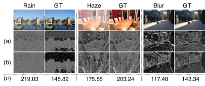
Figure 3: Absolute spatial derivatives of images in (a) vertical and (b) horizontal directions. (The values in the three color channels are summed together.) The values in the bottom are computed with the application of (1) on all the three color channels.

The dual residual networks employ an attention mechanism, which is the channel-wise attention that was originally developed for object recognition in the study of squeeze-and-excitation (SE) networks [26], and has been widely used for many other tasks. A SE-block computes and applies attention weights on the channels of the input feature map. To determine the weight on each channel, it computes the averages of activation values of channels; then, they are converted by two fully-connected layers with ReLU and sigmoid activaton functions to generate channel-wise weights. The aggregation of activation values is equivalent to global average pooling. We enhance this attention mechanism by incorporating a different aggregation method of channel activation.

Our idea is to use different statistics of channel activation values in addition to their averages. For this, we choose to use (absolute) spatial derivatives of channel activation values. More specifically, denoting an activation value at spatial position $(i,j)$ of channel $c$ by $y_{c,i,j}$, we calculate

$$\small v_{c}=\frac{1}{N}\sum_{i,j}\lvert y_{c,i+1,j}-y_{c,i,j}\rvert^{\beta}+\frac{1}{M}\sum_{i,j}\lvert y_{c,i,j+1}-y_{c,i,j}\rvert^{\beta},$$ (1)

where $N$ and $M$ denote the number of values in the corresponding spatial derivative maps; $\beta$(=3 for our experiments) is a scalar to enhance derivative values. This is also known as the total variation [54]. Figure 3 shows how the absolute spatial derivatives behaves for different inputs using input images (instead of intermediate layer features) as examples. It is observed that they provide different responses between clean and degraded images of the same scenes.

Figure 4 illustrates the proposed attention mechanism. We compute the global average and the total variation of activation values of each channel and input it to the same pipeline as the SE-block to generate attention weights over the channels. We replace the corresponding part in the SE-ResNet module with this reinforced attention mechanism. We will refer to the updated module as the “improved SE-ResNet module” in what follows. We will show the effectiveness of the above design though experiments including ablation tests.

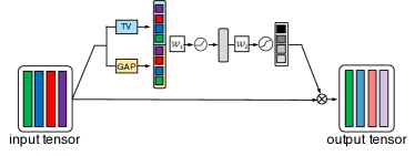
Figure 4: The proposed attention mechanism improving the SE block. It generates channel-wise attention weights by global average pooling (the same as the standard SE block) and total variation (TV) of each channel activation values.

3.1.2 Improved Design of a Dual Residual Block

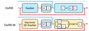
Figure 5: The proposed basic block (DuRB-M) used for building our network.

The design of the dual residual networks [42] aims at making maximum use of paired operations that are believed to fit for image restoration tasks. The choice of the paired operations is arbitrary and four choices are suggested depending on the type of degradations. We pay attention on the two of them, in both of which the first operation is up-convolution. Specifically, one is the pair of up-convolution (i.e., up-sampling followed by convolution) and simple convolution. The block employing the pair is named DuRB-U and applied to motion blur removal. (See the upper panel of Fig. 5.) The other is the pair of up-sampling followed by convolution and a SE-ResNet module. The block is named DuRB-US and applied to haze removal.

In this paper, aiming at development of a block structure that can deal with multiple degradation factors we propose a new design, which we call DuRB-M. The idea is to integrate the above two designs (i.e., DuRB-U and -US) and also replace the ResNet module in the original DuRB structure with the aforementioned improved SE-ResNet module. To be specific, while keeping the same up-convolution for the first operation, we employ parallel computation of the second operations of DuRB-U and -US, i.e., convolution and a SE-block, for the second operation of the new block design; see the lower panel of Fig. 5. The output maps of the two operations are merged by concatenation in the channel dimension, followed by $3\times 3$ convolution to adjust the number of channels.

3.2 Design of the Output Branches

Minimal Design   A minimal design of the output branches is to use a subnetwork of the same design but with different weights for each branch specific to a single degradation factor. Let $g_{i}$ $(i=1,\ldots)$ denote a subnetwork comprising one of the output branches. All $g_{i}$’s have an identical design, which starts with two sets of up-sampling plus convolution (implemented by PixelShuffle [57]) and ReLU in this order, followed by convolution with a hyperbolic tangent activation function. The internal convolution layers all employ $3\times 3$ kernels. The number of their channels are 96 for the first two conv. layers and 48 for the last one.

Improved Design

Although the above design works fairly well, further improvement can be achieved by inserting additional DuRB-M block(s), which is the same as those constituting the stem network, to some of the output branches. As shown in Fig. 2, the differences between different degradation factors are so large and they may not be fully absorbed by the lightweight $g_{i}$ of an identical design. We hypothesize that the difficulty with each degradation factor differs, and it can be handled by a hierarchical structure; easier factors are handled at a lower stage of the hierarchy and more difficult ones are at a higher stage. We conducted a systematic search, determining the following order for the primary four factors considered in this study: rain-streak, motion-blur, JPEG artifacts, and haze. To be specific, we stack three DuRB-M blocks in a row right after the stem network and insert $g_{i}$ ($i=1,2,3,4$) to each output of the stem network and the three stacked blocks; the inserted $g_{i}$’s handle the four factors in the above order.

3.3 Design of Input Branches

Although it is less essential to have multiple branches for the input of our network than for its output, we can achieve better performance by using different branches for the input. We adopt several ideas from the literature to design them. For motion blur, we employ the scale-recurrent [61] and selective parameter sharing [17] strategies, intending to restore clear textures progressively, and increase the capacity for removing various scales of blurring. We employ Gao et al. [17]’s implementation for this branch and accordingly update $g_{2}$ in the input branch. For haze removal, the basic design seems powerful enough [42]. For JPEG-noise removal, we employ the same strategy used for motion blur removal. Further details are given in supplementary material.

Table 1: An ablation test to evaluate the effectiveness of several components in the proposed block, DuRB-M. A single model is trained jointly on the four factors. PSNR/SSIM is shown.

	TV	GAP	Fusion	motion blur	haze	rain-streak	JPEG artifact
	✗	✗	✗	28.60 / 0.8698	30.00 / 0.9789	32.37 / 0.9136	28.13 / 0.8254
	✓	✗	✗	28.92 / 0.8778	32.35 / 0.9815	32.65 / 0.9162	28.14 / 0.8253
	✗	✓	✗	28.77 / 0.8737	32.48 / 0.9820	32.61 / 0.9150	28.14 / 0.8251
	✗	✗	✓	29.32 / 0.8853	33.80 / 0.9846	32.78 / 0.9186	28.15 / 0.8268
MBN	✓	✓	✓	29.35 / 0.8861	34.06 / 0.9860	32.83 / 0.9191	28.19 / 0.8271

4 Training Method

We train the proposed network in two steps. In the first step, we consider only its (non-recurrent) forward paths with different input-output branch pairs. We jointly train the forward paths on multiple degradation factors. After this step, the network can handle each degradation factor by using the corresponding input-output branch. In the second step, we fine-tune the network so that the network can deal with an image with unknown degradation factor by using the recurrent paths, as shown in Fig. 1.

4.1 Joint Training of Forward Paths

We first train our network in different forward paths jointly on multiple factors in the following way. We split the training process into a series of cycles, in each of which we train the network on a combination of all the degradation factors. To be specific, each cycle contains one or more randomly chosen minibatches of a single factor. Considering that the loss decreases at a different speed for different factors, we choose the number of minibatches in one cycle, specifically, one for haze removal, one for rain-streak removal, one for JPEG artifacts removal, and three for motion blur removal. The minibatches are randomly chosen from the training split of each dataset and packed in a random order in a row for the cycle. We then iterate this cycle until convergence. Each input image in a minibatch is obtained by randomly cropping a region from an original training image. The crop size is 128$\times$128 pixels and 256$\times$256 pixels for rain-streak and the other factors, respectively. Further details are given in the supplementary material.

4.2 Finetuning to Enable Recurrent Computation

After the joint training on the forward paths, we fine-tune the network so that it can be used in the recurrent computation mode. We first choose in what order the multiple degradation factors are processed in the recurrent path. We conduct a test to choose their order, as it affects the final performance; details will be given in Sec. 5.2. We then train the network on this recurrent path in the following way. Choosing a training sample of a degradation factor, we input it into the recurrent path. We then compute the loss for the final output against the ideal clean image. As we know the degradation factor of the input, we also compute the loss for the intermediate output at the corresponding output branch against the same clean image. We then compute a weighted sum of the two losses with fixed weights (0.8 for the intermediate output and 0.2 for the last output in our experiments), minimizing it by backpropagation as usual. Using a larger weight on the intermediate output, we intend to make the forward path specializing in that degradation factor continue to remove it, while guaranteeing that the other paths do no harm on the final results.

5 Experimental Results

5.1 Ablation Test on the DuRB-M Block

We have proposed two design improvements of the Dual Residual Block for multi-task learning. We present here an ablation study to evaluate the contribution of each design component. For this purpose, we train a number of networks with different configurations according to the training step of Sec. 4.1 on the same datasets of four degradation factors as Sec. 5.3. The stem net consists of five stacks of the DuRB-M block. For the sake of efficiency, we chose the minimal design for the output branches (Sec. 3.2) and identical design for the input branches (thus, there is only a single input branch). See the supplementary material for details. Table 1 shows the results. TV and GAP mean the channel-wise Total Variation and the channel-wise Global Average Pooling, respectively, both of which are used for attention computation. Fusion means the improved design of the dual residual block that employ fused operations (Sec. 3.1.2). It can be confirmed that the use of all the three components yields the maximum accuracy for all the factors.

5.2 Order of Factors in the Recurrent Path

In this study, we consider four degradation factors. Thus, the proposed network has four pairs of input-output branches. To examine the impact of the order of these factors processed in the recurrent path, we conducted an experiment. As exhaustive search needs tests on 24 order patterns, we employ a two-step approach. First, we choose three factors and test all the order patterns for them. Then, for the best order of the three factors, we insert the last factor into one of the four places. Table 2 shows the results; the first test on the three chosen factors, i.e., motion-blur, haze, and rain-streak is shown on the left and the second test on the last factor, i.e., JPEG noise on the right. It is seen that at least the orders of the first three factors have non-negligible effects. From the results, we choose the order J$\rightarrow$H$\rightarrow$B$\rightarrow$R for the subsequent experiments.

Table 2: Order of the degradation factors processed in the recurrent path. The results are averaged over three/four tasks.

order PSNR / SSIM B$\rightarrow$H$\rightarrow$R 31.83 / 0.9396 B$\rightarrow$R$\rightarrow$H 31.84 / 0.9395 H$\rightarrow$B$\rightarrow$R 32.07 / 0.9403 H$\rightarrow$R$\rightarrow$B 32.06 / 0.9402 R$\rightarrow$B$\rightarrow$H 31.81 / 0.9128 R$\rightarrow$H$\rightarrow$B 32.02 / 0.9401 order PSNR / SSIM J$\rightarrow$H$\rightarrow$B$\rightarrow$R 31.14 / 0.9123 H$\rightarrow$J$\rightarrow$B$\rightarrow$R 31.13 / 0.9121 H$\rightarrow$B$\rightarrow$J$\rightarrow$R 31.12 / 0.9121 H$\rightarrow$B$\rightarrow$R$\rightarrow$J 31.13 / 0.9121

Table 3: Comparison of the proposed method (MBN/R-MBN) with state-of-the-art methods on the removal task of each of four degradation factors (PSNR/SSIM). Methods in the “dedicated” block are designed for a single degradation factor. MBN is trained on all the factors but requires specification of the target factor. R-MBN and cascade do not need it. The best one is in bold and the second is with underline.

baselines	motion blur removal		haze removal		rain-streak removal		JPEG artifacts removal (q=10)
dedicated	Liu et al. [42]	29.90 / 0.9100	Cai et al. [5]	19.82 / 0.82	Wang et al. [65]	30.05 / 0.93	Dong et al. [14]	28.98 / 0.82
	Zhang et al. [81]	30.63 / 0.9053	Ren et al. [53]	24.91 / 0.92	Li et al. [37]	32.48 / 0.91	Chen et al. [11]	29.15 / 0.81
	Purohit et al. [49]	30.79 / 0.9100	Liu et al. [42]	32.12 / 0.98	Li et al. [35]	33.16 / 0.92	Zhang et al. [85]	29.19 / 0.81
	Gao et al. [17]	31.35 / 0.9174	Liu et al. [41]	32.16 / 0.98	Liu et al. [42]	33.21 / 0.93	Zhang et al. [87]	29.63 / 0.82
MBN	30.70 / 0.9111		32.68 / 0.98		33.40 / 0.93		28.24 / 0.83
cascade	17.48 / 0.7306		27.03 / 0.87		21.52 / 0.76		16.97 / 0.64
R-MBN	30.67 / 0.9110		32.38 / 0.98		33.40 / 0.93		28.19 / 0.83

Table 4: Results of restoration from images with mixed degradation factors. R-MBN is trained only on images with a pure, uncombined factor. R-MBN* and Suganuma et al. [58] are trained on images with mixed factors.

	rain	blur	haze	JPEG	R-MBN	R-MBN∗	Suganuma et al. [58]
One task	✓	✗	✗	✗	38.63 / 0.9797	34.84 / 0.9684	30.50 / 0.8660
	✗	✓	✗	✗	33.66 / 0.9525	31.41 / 0.9429	27.55 / 0.8411
	✗	✗	✓	✗	30.07 / 0.9710	30.61 / 0.9747	25.73 / 0.9019
	✗	✗	✗	✓	31.72 / 0.9154	30.89 / 0.9127	28.99 / 0.8584
Two tasks	✓	✓	✗	✗	28.59 / 0.8454	29.91 / 0.9072	26.13 / 0.7853
	✓	✗	✓	✗	28.42 / 0.9441	28.41 / 0.9451	24.12 / 0.8139
	✓	✗	✗	✓	25.66 / 0.7515	29.25 / 0.8753	27.18 / 0.7828
	✗	✓	✓	✗	26.58 / 0.9163	27.57 / 0.9216	23.27 / 0.7776
	✗	✓	✗	✓	26.90 / 0.8012	27.42 / 0.8292	26.04 / 0.7714
	✗	✗	✓	✓	24.89 / 0.8548	26.60 / 0.8693	24.42 / 0.8075
Three tasks	✓	✓	✓	✗	22.57 / 0.7894	26.12 / 0.8786	22.38 / 0.7195
	✓	✓	✗	✓	23.64 / 0.6912	26.20 / 0.7879	24.91 / 0.7214
	✓	✗	✓	✓	21.15 / 0.7045	25.23 / 0.8269	22.04 / 0.6732
	✗	✓	✓	✓	21.29 / 0.7154	24.71 / 0.7843	22.59 / 0.7117
Four tasks	✓	✓	✓	✓	18.84 / 0.6249	23.58 / 0.7436	22.04 / 0.6733
	Random combinations				25.41 / 0.7881	27.37 / 0.8502	24.58 / 0.7618

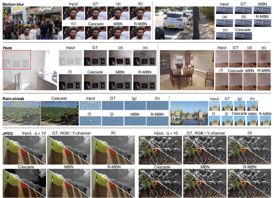
Figure 6: Qualitative comparison on the four degradation factors. Motion blur: (a) [81]; (b) [17]; (c) [42]. Haze: (d) [53]; (e) [41]; (f) [42]. Rain-streak: (g) [37]; (h) [35]; (i) [77]; (j) [42]. JPEG artifact: (k) [87]. “Cascade” is the cascade of four models as in Table 3.

5.3 Performance on Single Factor Removal

We first show the performance of our models on single factor removal tasks. We consider two models. One is the model obtained right after the first training step, which has multiple input-output pairs. The other is the final model obtained after the fine-tuning, which has a single input and output. Their difference is whether we need to specify the degradation factor of the input images or not.

Datasets   We choose dataset(s) for each task that is the most widely used in recent studies. We use the GoPro dataset [46] for motion blur removal. It consists of 2,013 and 1,111 non-overlapped training (GoPro-train) and test (GoPro-test) pairs of blurred and sharp images, respectively. We use the RESIDE dataset [34] for haze removal, which consists of 13,990 samples of indoor scenes and a few test subsets. Following [42] and [53], we use a subset SOTS (Synthetic Objective Testing Set) that contains 500 indoor scene samples for evaluation. We use the DID-MDN dataset [83] for rain-streak removal. It consists of 12,000 training pairs and 1,200 test pairs of clear image and synthetic rainy image. As for JPEG artifacts removal, we use the training subset (800 images) of the DIV2K dataset [63] and LIVE1 dataset (29 images) for training and testing our networks, following the study of the state-of-the-art method [87].

Results   Table 3 shows the results. It includes the performance of four best published methods for each degradation factor (“dedicated”). We use the authors’ codes for them. MBN indicates our model after the 1st training step and R-MBN indicates our model after the fine-tuning. As a baseline of the latter, we consider a cascade of the four best dedicated models (i.e., the last row in the “dedicated” block), which at least formally does not need specification of a degradation factor. To be specific, we cascade the models of Zhang et al. [87]’s, Liu et al. [42]’s, Gao et al. [17]’s, and Liu et al. [42] in this order (J$\rightarrow$H$\rightarrow$B$\rightarrow$R).

It is seen from the table that MBN yields at least comparable performance to the best dedicated models. More importantly, R-MBN, which has only a single input and output and thus can deal with images with any degradation factor, achieves very similar performance to MBN. This will be a big advantage in real world applications, despite some gap with the best dedicated model (e.g., motion blur). Figure 6 shows a few examples of restoration from each of the four factors. It can be observed that the proposed MBN can restore high-quality images comparable to the state-of-the-art methods, and R-MBN attains similar quality to MBN. These agree well with the above quantitative comparison. It is also seen that the cascade of the four networks yield only sub-optimal results. For JPEG, we show RGB images as well as Y-channel images, as the latter are mainly used in the previous studies including RNAN [87]. It is seen from the restored RGB images that our networks recover more precise colors.

5.4 Removal of Unknown Combined Degradations

An even harder task is to restore images with mixed degradation factors with unknown mixing ratios. We tested two versions of our model on this task. One is the model trained by the aforementioned method on training images having a single degradation factor, i.e., R-MBN in Table 3. We also train the same network on a set of images with mixed degradation factors, which are generated as explained below. We refer to it as “R-MBN*”. We compare these with the method of Suganuma et al. [58], for which, following their paper, we train their network on the same set of images with mixed degradation factors. We omit the results of the earlier study [80] on this task, since they perform worse than [58], as is reported in [58].

Dataset   Since the datasets used in the previous studies [80, 59] are not fit for the purpose here, we created a new dataset covering the same four degradation factors. For this purpose, we use the outdoor scenes in RESIDE-$\beta$ [34], which is the dataset for haze removal, as source images and add synthesized degradation to them. We synthesize motion blur effects, rain-streak effects, and JPEG artifacts by the method of Hendrycks et al. [24], GIMP on Ubuntu 18.04.2 [62], and the Python Imaging Library, respectively. For haze, we use the original data in the RESIDE-$\beta$ dataset. Then, we create two training datasets; a set of images with a pure degradation factor out of the four and a set of images with combined degradation factors. For the latter, we create each image so that it has a combination of $X$ factors, where $X$ is a random number chosen from $\{1,2,3,4\}$. We create two groups of test sets associated with the two training datasets. The first group contains four test sets of images with a pure degradation factor and the second group contains twelve test sets covering all the combinations of either two, three, or four factors; see Table 4. Further details are given in the supplementary material.

Experiments   We consider two versions of our model trained differently; they have the same architecture as the last experiment. The first model is trained on the training set of pure, uncombined factors by the aforementioned two-step method. The second model is obtained by fine-tuning the first one from its first step’s checkpoint on the training set of combined factors. The method of Suganuma et al. is also trained on them, following the suggested method in their paper. Then we test the three models on all the test sets, i.e., the four of pure factors and the twelve of combined factors.

Results   Table 4 shows the results. It is seen that unsurprisingly, our model trained on single-factor data (R-MBN) achieves the best performance on single-factor test sets; and that trained on combined-factor data (R-MBN*) achieves the best performance on combined-factor test sets. More importantly, the latter outperforms the method of Suganuma et al. with large margins, while it is not so inferior to the model trained on pure factors (R-MBN). Thus, from a practical application point of view, R-MBN* will be the first choice for images having combined factors and R-MBN is recommended for images with a single factor. Additionally, although R-MBN is inferior to R-MBN* in the case of combined factors, the gap is not so large up to combination of two factors, and it is still mostly better than the method of Suganuma et al. Considering the fact that R-MBN is trained only on images with pure factors, this result is encouraging for a further study toward “universal image restoration method” that can handle any degradation factors including those that have not seen before.

6 Conclusion

In this paper, we have considered the problem of restoring a clean image from its degraded version with an unknown degradation factor, subject to the condition that it is one of the known factors. To solve this problem, we proposed a network having multiple pairs of input and output branches and use it in a recurrent fashion such that a different branch pair is used at each of the recurrent paths. The shared part of the network is build upon dual residual networks recently proposed by Liu et al. We showed improved designs of its component block, named DuRB-M, that enables to handle different degradation factors. We have also proposed a two-step training method for the network, which consists of multi-task learning and fine-tuning. We showed through several experimental results the effectiveness of the proposed method.

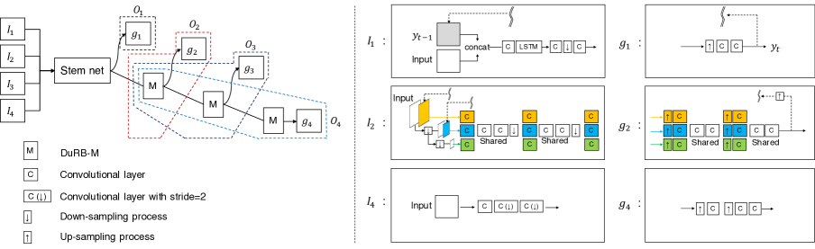
Figure 7: An illustration of the architecture of the proposed network with the optimized input/output branches. ($I_{1},O_{1}$) is used for rain-streak. ($I_{2},O_{2}$) is for motion-blur. ($I_{3},O_{3}$) is for JPEG artifacts. $(I_{4},O_{4})$ is for haze.

Appendix

Appendix A Detailed Design of Input/Output Branches

The input-output branch pairs comprising the proposed network can have different designs for different degradation factors, as they are specifically used for an individual factor. The network works fairly well even when employing the same design (but with unshared weights) for all the factors considered in this study. However, as explained in the main paper, the network with factor-specific input/output branches achieves the best performance; the results reported in Sec.5.3 and 5.4 were obtained by one such design. In the main paper, we provide only a brief summary about it due to the lack of space. Here, we provide its details as well as underlying thoughts and experiments conducted to validate its design.

A.1 Hierarchical Design of Output Branches

Figure 7 shows the the proposed network with the complete illustration of all the branches. As briefly explained in Sec. 3.3, we employ a hierarchical design utilizing additional DuRB-M blocks in the design of output branches for different factors, as shown in the upper-left of Fig. 7. We found this design to performs the best in an experiment, where we compared possible configurations of three factors shown Fig. 8; we chose the three factors ( motion blur, haze, and rain-streak) for the sake of efficiency.

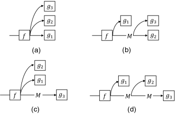
Figure 8: Possible configurations of output branches with additional DuRB-M blocks. M indicates a DuRB-M block. Note that we consider configurations of selected three factors in our comparative experiments for the sake of efficiency.

Assuming the above result applies to the case of four factors, we ran a systematic search to find the best alignment of $g_{1},\ldots,g_{4}$ and the four factors. As there are 24 ways of alignment in total, we employ the following two-step search strategy for the sake of efficiency. We first search for the optimal alignment for three selected factors, motion blur, haze, and rain-streak. We then consider inserting JPEG artifacts (J) into the best alignment of the three factors. To make this search efficient, we also employ an identical design for the input branches as well as output branches for all the factors. The former consists of three conv. layers with $48$, $96$, and $96$ channels and with stride $=1$, 2, and 2, respectively. For the latter, we use the minimal design introduced in Sec. 3.2 for all $g_{i}$’s ($i=1,2,3,4$).

Table 5 shows the results of the first stage of this search. ‘$\rightarrow$’ indicates a DuRB-M block. It is seen that R$\rightarrow$B$\rightarrow$H performs the best. We then test inserting J into R$\rightarrow$B$\rightarrow$H, as shown in Table 6. Based on the results, we choose R$\rightarrow$B$\rightarrow$J$\rightarrow$H. Note that this ‘order’ of the factors in the network design is different from the order of the degradation factors processed in a recurrent path, which is chosen to be J$\rightarrow$H$\rightarrow$B$\rightarrow$R, as is explained in Sec. 5.2; that is, J is first removed by using the corresponding input/output pair, next H is removed by using the corresponding pair, similarly, B and R.

Table 5: B: motion-blur removal, H: haze removal, and R: rain-streak removal. The values (PSRN/SSIM are averaged accuracy over the three tasks.

Alignment PSNR / SSIM B$\rightarrow$H$\rightarrow$R 30.61 / 0.9244 B$\rightarrow$R$\rightarrow$H 30.42 / 0.9227 H$\rightarrow$B$\rightarrow$R 30.57 / 0.9244 H$\rightarrow$R$\rightarrow$B 30.34 / 0.9219 R$\rightarrow$B$\rightarrow$H 30.79 / 0.9246 R$\rightarrow$H$\rightarrow$B 30.29 / 0.9201

Alignment PSNR / SSIM BH$\rightarrow$R 30.24 / 0.9217 B$\rightarrow$HR 30.36 / 0.9216 HR$\rightarrow$B 30.02 / 0.9189 H$\rightarrow$RB 30.41 / 0.9236 RB$\rightarrow$H 30.47 / 0.9219 R$\rightarrow$BH 30.38 / 0.9228 RBH 30.32 / 0.9206

Table 6: B: motion-blur removal, H: haze removal, and R: rain-streak removal. The values (PSRN/SSIM are averaged accuracy over the three tasks.

Alignment PSNR / SSIM J$\rightarrow$R$\rightarrow$B$\rightarrow$H 30.09 / 0.8997 R$\rightarrow$J$\rightarrow$B$\rightarrow$H 30.18 / 0.9004 R$\rightarrow$B$\rightarrow$J$\rightarrow$H 30.22 / 0.8995 R$\rightarrow$B$\rightarrow$H$\rightarrow$J 30.17 / 0.9004

Alignment PSNR / SSIM JR$\rightarrow$B$\rightarrow$H 30.20 / 0.8985 R$\rightarrow$BJ$\rightarrow$H 30.13 / 0.8991 R$\rightarrow$B$\rightarrow$HJ 30.02 / 0.8995

A.2 Specific Design for Each Degradation Factor

Based on the above experiment (i.e., Table 6), we use the input/output pair $(I_{1},O_{1})$ for rain-streak, $(I_{2},O_{2})$ for motion blur, $(I_{3},O_{3})$ for JPEG artifacts, and $(I_{4},O_{4})$ for haze, respectively, as shown in Fig. 7. We explain the design of each branch pair below.

A.2.1 Rain-streak

We adopt the design of [51]. The input branch $I_{1}$ consists of a ConvLSTM module and two convolutional layers. The ConvLSTM module consists of a convolutional layer with 32 channels and a LSTM, which has four units with 32 channels. The subsequent two convolutional layers have 64 and 96 channels, respectively, in between which there is a $\times 1/2$ down-sampling layer. We use $3\times 3$ kernels for all the convolutional layers in $I_{1}$. The output branch $O_{1}$, which consists only of $g_{1}$, is designed to be symmetric to $I_{1}$; $g_{1}$ consists of a [conv.+up-sampling] and two conv. layers. These three conv. layer have 96, 48, and 3 channels, respectively.

A.2.2 Motion Blur

We adopt the design of [17]. The input branch $I_{2}$ contains three internal branches, so does $O_{2}$. The whole network is recurrently used (within the motion blur removal task) by using these three internal input-output pairs. Specifically, the input image is first down-sampled by the factor of 1/4 and inputted to one of the three. The output from the corresponding internal output branch is then fed back to the second internal input branch, where it is concatenated in the channel dimension with the original image down-sampled by the factor of 1/2. This is repeated once more, yielding the final result.

As shown in Fig. 7, $I_{2}$ (after the down-sampling) starts with three parallel conv. layers followed by two conv. layers and a $\times 1/2$ down-sampling layer. These conv. layers have 32 channels. For down-sampling, we use Pixel-unshuffle. After these, $I_{2}$ proceeds with another set of three parallel conv. layer, two conv. layer, and a $\times 1/2$ down-sampling layer. These conv. layers all have 64 channels. Finally, $I_{2}$ ends with another set of three parallel conv. layers with 96 channels. $I_{1}$ has 13 conv. layers in total, each of which has $3\times 3$ kernels and a subsequent ReLU layer.

The output branch $O_{2}$ consists of one DuRB-M block and $g_{2}$, and the latter has a symmetric structure to $I_{2}$. As shown in Fig. 7, $g_{2}$ starts with three parallel paths consisting of a $\times 2$ up-sampling layer with a built-in conv. layer (w/ 96 channels) and a conv. layer (w/ 64 channels) followed by two additional conv. layers (w/ 64 channels). The same structure is repeated once (channels of the conv. layers are 64, 32, and 32, respectively), connecting to the output. All the conv. layers use 3$\times$3 kernels. A ReLU layer follows every conv. layer except the one employed in each up-sampling module.

A.2.3 JPEG Artifacts

The output branch $O_{3}$ consists of a series of two DuRB-M blocks followed by $g_{3}$. We use the same design for $I_{3}$ and $g_{3}$ as $I_{2}$ and $g_{2}$, respectively. We found this works well for this factor.

A.2.4 Haze

The output branch $O_{4}$ consists of a series of three DuRB-M blocks followed by $g_{4}$. For $I_{4}$ and $g_{4}$, we employ the minimal design explained in the main paper, as shown in Fig. 7.

Table 7: The number of parameters and the memory footprint of the three sections of the proposed network, i.e., the input branches, the stem network, and the output branches, for the model with the minimal design of the input/output branches and the model with the improved design.

# of param.	input	stem	output
minimal design	0.07M	3.94M	0.52M
improved design	2.35M	3.94M	4.96M
GPU memory	input	stem	output
minimal design	0.3MB	15.76MB	2.08MB
improved design	9.43MB	15.76MB	19.87MB

Table 8: The number of parameters and the memory footprint of each component of the proposed network. M_i indicates a DuRB-M block.

minimal # of param. memory in-branch conv.$\times$3 0.07 (M) 0.3 (MB) stem M1 0.64 15.76 M2 0.74 M3 0.74 M4 0.84 M5 0.98 out-branch g1 0.13 2.08 (=0.52$\times 4$) g2 0.13 g3 0.13 g4 0.13

improved # of param. memory in-branch $I_{1}$ 0.32 (M) 1.26 (MB) $I_{2}$ 0.98 3.93 $I_{3}$ 0.98 3.93 $I_{4}$ 0.07 0.3 stem M1 0.64 15.76 M2 0.74 M3 0.74 M4 0.84 M5 0.98 out-branch g1 0.04 0.16 M${}_{6}+$g2 0.98 + 0.48 5.86 M${}_{6}+$M${}_{7}+$g3 0.98+1.43+0.48 11.56 M${}_{6}+$M${}_{7}+$M${}_{8}+$g4 0.98+1.43+1.43+0.13 15.87

A.3 Number of parameters

Our network is composed of the input branches, the stem network, and the output branches. The motivation behind this composition is to make it possible to deal with multiple degradation factors with a compact network. The network is recurrently used, in which each input/output branch pair is specifically used for a single factor while the stem network is used for all the factors. Table 7 shows the number of parameters and memory footprint for the three sections for two different designs, i.e., the minimal design and the improved design; the latter was used for the experiments of Sec. 5.3 and 5.4. Table 8 shows those for each component of the networks. It is seen from Table 7 that the improved design of input/output branches needs a lot more parameters and memory as compared with the minimal design; however they are still comparable to those needed by the stem network. Considering that the network deals with the four different degradation factors, we think this is acceptable.

Appendix B Details of Training

Global Settings

We use the Adam optimizer with $(\beta_{1},\beta_{2})=(0.9,0.999)$ and $\epsilon=1.0\times 10^{-8}$ for training all the models. For loss functions, we use a weighted sum of SSIM and $l_{1}$ loss, specifically, $1.1\times$SSIM$+0.75\times l_{1}$ following Liu et al.’s setting [42], for all the tasks. The initial learning rate is set to 0.0001 for all the tasks. All the experiments are conducted using PyTorch. Our code and trained models is publicly available (https://github.com/6272code/6272-code). For data augmentation, we use horizontal flip for the removal of motion blur, rain-streak, and JPEG artifacts; for haze, we use horizontal and vertical flips, and image rotations with a degree randomly chosen from $[90,180,270]$.

Training MBN (Sec. 5.3)

We set the size of minibatch to $40$ for training the network. We reduced learning rate by $\times 0.1$ twice at the iterations where the training loss stopped decreasing. The model is trained $1.2\times 10^{5}$ iterations. By an iteration, we mean a cycle (i.e., a set of multiple minibatches containing different factors), as explained in Sec. 4.1. The crop size is $128\times 128$ and $256\times 256$ pixels for rain-streak and the other factors, respectively.

Training R-MBN (Sec. 5.3)

We fine-tuned the MBN model. The learning rate was set to be 0.000001 for the training. We fixed parameters of all the input branches to accelerate training. The crop size is $128\times 128$ and $256\times 256$ pixels for rain-streak and the other factors, respectively. We stopped the fine-tuning when the training loss stopped decreasing. The size of minibatches was set to $4$.

Configuration for Systematic Search of Output Branches

The models are trained for $1\times 10^{5}$ iterations with batchsize $=3$. We resize the images of GoPro dataset and DIV to $\times 1/2$ for training to reduce memory usage. Note that this configuration is used only here. We use the crop size of $256\times 256$ pixels for all the models.

Training Details for Ablation Tests1 (Sec. 5.1)

We employ the model having the best design of output branches found by the systematic search. We train all the models for $5\times 10^{4}$ iterations with batchsize $=20$. We set crop size to $256\times 256$ pixels for all the models here.

Training Details for Ablation Tests2 (Sec. 5.2)

We use batchsize $=4$ and learning rate $=0.000001$. All the models are fine-tuned for $1\times 10^{4}$ iterations starting from the checkpoint at the $8\times 10^{4}$ iteration of training of MBN used in Table 3. For crop size, we use $256\times 256$ pixels for motion blur, haze and JPEG artifacts, and $128\times 128$ for rain-streak.

Training Details for Removal of Unknown Combined Degradations

We have trained two versions of the proposed model, i.e., R-MBN and R-MBN*. For R-MBN, we trained it on uncombined single-factor data with the proposed two-step training method. The crop size is $128\times 128$ pixels and $256\times 256$ pixels for rain-streak and the other factors, respectively. The model was trained for $8.5\times 10^{4}$ iterations in the first step, and for $2.5\times 10^{4}$ iterations in the second step. For R-MBN*, we fine-tuned the model on the training set of combined factors with crop size of $256\times 256$ pixels, starting from a checkpoint of the training of R-MBN. We fixed the parameters of all the input branches to accelerate training. This version was also trained for $2.5\times 10^{4}$ iterations.

Appendix C Data Used for Experiments on Unknown Combined Degradations (Sec. 5.4)

As noted in the main paper, we created a dataset for the experiments on removal of unknown combined degradation factors. This dataset is created from the 8,970 outdoor scenes provided in RESIDE-$\beta$ [34]. We split the scenes into 8,478 and 492 and use the former for training and the latter for test. The test set contains the same images used in the synthetic-objective-test (SOTS), which is a popular benchmark test set of RESIDE. We then synthesize pure degradation on the aforementioned training and test images, yielding two training subsets and 16 test subsets, as explained in Sec. 5.4 of the main paper.

Synthesis of Motion Blur

We employ Hendrycks et al.’s approach [24] to synthesize motion blur. The (radius, sigma) used in the approach are randomly chosen from $\{(10,1.5),(10,2.5),(12,3),(12,3.5),(13,8),(15,12)\}$ for each input. The angle of motion blur is randomly generated according to the uniform distribution with the range [-45,45] (in degrees).

Synthesis of Rain-streak

We followed a tutorial on the creation of rain-streak effects. The rain-streaks are synthesized by motion-blurring Gaussian noise on an image by GIMP on Ubuntu 18.04.2. For each image, we randomly choose a noise level from $[0.55,0.65,0.7,0.8]$ for generating Gaussian noise; we decide the magnitude of motion blur (motion blur length) by randomly selecting a value from $\{10,20,35,50\}$. The direction of rain-streaks for an image is randomly chosen by randomly selecting a motion blur’s angle from $\{110,105,100,90,85,80,70\}$ (in degrees).

Synthesis of JPEG Artifacts

We simply compress each image by JPEG. To be specific, we use Pillow, i.e., $\mathtt{PIL.Image.save(buff,quality=X)}$. The compression quality is chosen for each image from the range of $[15,16,\dots,50]$.

Synthesis of Haze

RESIDE-$\beta$ consists of a large number of clean images and their hazy versions with different haze levels. There are two parameters ($v_{1}$ and $v_{2}$) used for generating hazy effects in the RESIDE-$\beta$ dataset: $v_{1}\in\{1,0.95,0.9,0.8,0.85\}$ and $v_{2}\in\{0.2,0.16,0.12,0.1,0.08,0.06,0.04\}$. For each clean image, there are 35 ($=5\times 7$, all the combinations of $v1$ and $v2$) hazy versions in the dataset. We use these images for our purpose; specifically, for each clean image, we randomly choose $v_{1}$ from the above set, and $v_{2}$ from $\{0.2,0.16,0.12,0.1,0.08\}$.

Order of Synthesis

When applying the above effects on an image, their order is important. Considering a natural process of image formation, we employ the following order: haze, rain-streak, motion blur, JPEG artifacts. This order applies to all the cases of combining two, three, four, and random number factors. Examples of the synthesized images are shown in Fig. 9 and 10.

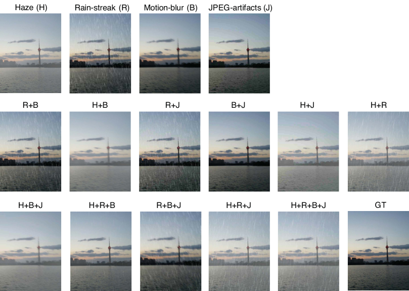
Figure 9: Examples of the images with synthetic degradation. These are used in the experiment of Sec. 5.4 of the main paper.

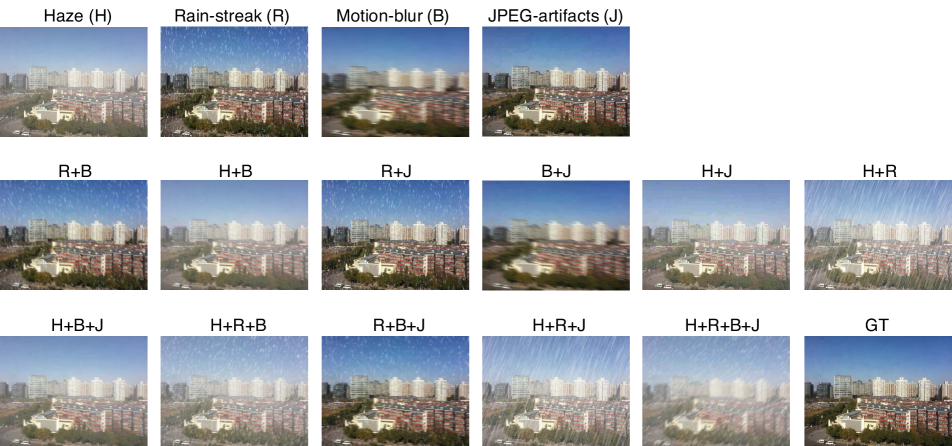
Figure 10: Examples of the images with synthetic degradation. These are used in the experiment of Sec. 5.4 of the main paper.

Appendix D Examples of Restoration from Combined Degradation (Sec. 5.4)

In Sec. 5.4 of the main paper, we evaluate the performances of several methods using the dataset created as above. Figure 11 shows several examples of the results obtained by the proposed methods (R-MBN and R-MBN*) and the baseline (Suganuma et al. [58]), which are omitted in the main paper due to lack of space. R-MBN is trained on images with a single degradation factor, whereas R-MBN* is trained on images with mixed degradation factors. In the last two rows of the figure, we show the outputs of an object detector (YOLO-v3) applied to each image, i.e., the original input, the restored images by the methods, and the ground-truth image.

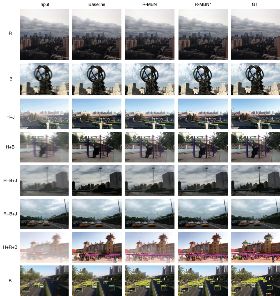
Figure 11: Qualitative evaluation of the proposed method (R-MBN and R-MBN*) and the compared baseline (i.e., Suganuma et al. [58]). R, B, J and H means rain-streak, motion blur, JPEG artifacts, and haze. R-MBN and R-MBN* are the proposed models. Object detection is performed by YOLO-v3.

References

- [1] D. Babacan, R. Molina, M. Do, and A. Katsaggelos. Bayesian blind deconvolution with general sparse image priors. In ECCV, 2012.
- [2] D. Berman, T. Treibitz, and Sh. Avidan. Non-local image dehazing. In CVPR, 2016.
- [3] D. Berman, T. Treibitz, and Sh. Avidan. Air-light estimation using haze-lines. In ICCP, 2017.
- [4] K. Bredies and M. Holler. A total variation-based jpeg decompression model. SIAM Journal on Imaging Sciences, 5(1):366–393, 2012.
- [5] B.L. Cai, X.M. Xu, K. Jia, C.M. Qing, and D.C. Tao. Dehazenet: An end-to-end system for single image haze removal. IEEE Transactions on Image Processing, 25(11):5187–5198, 2016.
- [6] J.R. Cai, W.M. Zuo, and L. Zhang. Extreme channel prior embedded network for dynamic scene deblurring. In arXiv, preprint arXiv:1903.00763, 2019.
- [7] R. Caruana. Multitask learning. Machine Learning, 28(1):41–75, 1997.
- [8] H.B. Chang, M.K. Ng, and T.Y. Zeng. Reducing artifacts in jpeg decompression via a learned dictionary. IEEE Transactions on Signal Processing, 62(3):718–728, 2014.
- [9] F. Chen, L. Zhang, and H.M. Yu. External patch prior guided internal clustering for image denoising. In ICCV, 2015.
- [10] Y.L. Chen and C.T. Hsu. A generalized low-rank appearance model for spatio-temporally correlated rain streaks. In ICCV, 2013.
- [11] Y.J. Chen and T. Pock. Trainable nonlinear reaction diffusion: A flexible framework for fast and effective image restoration. IEEE Transactions on Pattern Analysis and Machine Intelligence, 39(6):1256–1272, 2017.
- [12] H.J. Cheong, E.J. Chae, E.S. Lee, G.H. Jo, and J. Paik. Fast image restoration for spatially varying defocus blur of imaging sensor. Sensors, 15(1):880–898, 2015.
- [13] K. Dabov, A. Foi, V. Katkovnik, and K. Egiazarian. Image denoising by sparse 3-d transform-domain collaborative filtering. IEEE Transactions on Image Processing, 16(8):2080–2095, 2007.
- [14] C. Dong, Y Deng, C. Change Loy, and X.O. Tang. Compression artifacts reduction by a deep convolutional network. In ICCV, 2015.
- [15] R. Fergus, B. Singh, A. Hertzmann, S. Roweis, and W. Freeman. Removing camera shake from a single photograph. ACM Transactions on Graphics, 25(3):787–794, 2006.
- [16] L. Galteri, L. Seidenari, M. Bertini, and A.D. Bimbo. Deep generative adversarial compression artifact removal. In ICCV, 2017.
- [17] H.Y. Gao, X. Tao, X.Y. Shen, and J.Y. Jia. Dynamic scene deblurring with parameter selective sharing and nested skip connections. In CVPR, 2019.
- [18] D. Gong, J. Yang, L.Q. Liu, Y.N. Zhang, I. Reid, C.H. Shen, A.D. Hengel, and Q.F. Shi. From motion blur to motion flow: A deep learning solution for removing heterogeneous motion blur. In CVPR, 2017.
- [19] M. González, J. Preciozzi, P. Musé, and A. Almansa. Joint denoising and decompression using cnn regularization. In CVPR Workshops, 2018.
- [20] I. Goodfellow, J. Pouget-Abadie, M. Mirza, B. Xu, D. Warde-Farley, S. Ozair, A. Courville, and Y. Bengio. Generative adversarial nets. In NeurIPS, 2014.
- [21] W. Han, S.Y. Chang, D. Liu, M. Yu, M. Witbrock, and T. Huang. Image super-resolution via dual-state recurrent networks. In CVPR, 2018.
- [22] K.M. He, G. Gkioxari, P. Dollar, and R. Girshick. Mask r-cnn. In ICCV, 2017.
- [23] K.M. He, J. Sun, and X.O. Tang. Single image haze removal using dark channel prior. IEEE Transactions on Pattern Analysis and Machine Intelligence, 33(12):2341–2353, 2011.
- [24] D. Hendrycks and T. Dietterich. Benchmarking neural network robustness to common corruptions and perturbations. In ICLR, 2019.
- [25] N. Hideki and N. Michiharu. Local map estimation for quality improvement of compressed color images. Pattern Recognition, 44(4):788–793, 2011.
- [26] J. Hu, L. Shen, and G. Sun. Squeeze-and-excitation networks. In CVPR, pages 7132–7141, 2018.
- [27] N. Johnston, D. Vincent, D. Minnen, M. Covell, S. Singh, T. Chinen, S. Jin Hwang, J. Shor, and G. Toderici. Improved lossy image compression with priming and spatially adaptive bit rates for recurrent networks. In CVPR, 2018.
- [28] L.W. Kang, C.W. Lin, and Y.H. Fu. Automatic single-image-based rain streaks removal via image decomposition. IEEE Transactions on Image Processing, 21(4):1742–1755, 2012.
- [29] R. Kanthan and N. Sujatha. Rain drop detection and removal using k-means clustering. In ICCIC, 2015.
- [30] A. Kendall, Y. Gal, and R. Cipolla. Multi-task learning using uncertainty to weigh losses for scene geometry and semantics. In CVPR, 2018.
- [31] I. Kligvasser, T.R. Shaham, and T. Michaeli. xunit: Learning a spatial activation function for efficient image restoration. In CVPR, 2018.
- [32] O. Kupyn, V. Budzan, M. Mykhailych, D. Mishkin, and J. Matas. Deblurgan: Blind motion deblurring using conditional adversarial networks. In CVPR, 2018.
- [33] H. Kurihata, T. Takahashi, I. Ide, Y. Mekada, H. Murase, Y. Tamatsu, and T. Miyahara. Rainy weather recognition from in-vehicle camera images for driver assistance. In IVS, 2005.
- [34] B.Y. Li, W.Q. Ren, D.P. Fu, D.C. Tao, D. Feng, W.J. Zeng, and Z.Y. Wang. Reside: A benchmark for single image dehazing. In arXiv, preprint arXiv:1712.04143, 2017.
- [35] G.B. Li, X. He, W. Zhang, H.Y. Chang, L. Dong, and L. Lin. Non-locally enhanced encoder-decoder network for single image de-raining. In Proc. ACM-MM, 2018.
- [36] R.T. Li, L.F. Cheong, and R.T. Tan. Heavy rain image restoration: Integrating physics model and conditional adversarial learning. In CVPR, 2019.
- [37] X. Li, J.L. Wu, Z.C. Lin, H. Liu, and H.B. Zha. Recurrent squeeze-and-excitation context aggregation net for single image deraining. In ECCV, 2018.
- [38] Y. Li, R. Tan, X.J. Guo, J.B. Lu, and M. Brown. Rain streak removal using layer priors. In CVPR, 2016.
- [39] B. Lim, S.H. Son, H.W. Kim, S.J. Nah, and K.U. Mu Lee. Enhanced deep residual networks for single image super-resolution. In CVPR workshops, 2017.
- [40] J.Y. Liu, W.H. Yang, S. Yang, and Z.M. Guo. Erase or fill? deep joint recurrent rain removal and reconstruction in videos. In CVPR, 2018.
- [41] X.H. Liu, Y.R. Ma, Z.H. Shi, and J. Chen. Griddehazenet: Attention-based multi-scale network for image dehazing. In ICCV, 2019.
- [42] X. Liu, M. Suganuma, Z. Sun, and T. Okatani. Dual residual networks leveraging the potential of paired operations for image restoration. In CVPR, 2019.
- [43] Y. Liu, Z.W. Wang, H.L. Jin, and I. Wassell. Multi-task adversarial network for disentangled feature learning. In CVPR, 2018.
- [44] T. Martyniuk. Multi-task learning for image restoration. Master’s thesis, Ukrainian Catholic University, 2019.
- [45] G.F. Meng, Y. Wang, J.Y. Duan, S.M. Xiang, and C.H. Pan. Efficient image dehazing with boundary constraint and contextual regularization. In ICCV, 2013.
- [46] S. Nah, T.H. Kim, and K.M. Lee. Deep multi-scale convolutional neural network for dynamic scene deblurring. In CVPR, 2017.
- [47] J.S. Pan, Z. Hu, Z.X. Su, and M.H. Yang. Deblurring text images via l0-regularized intensity and gradient prior. In CVPR, 2014.
- [48] Y.R. Piao, W. Ji, J.J. Li, M. Zhang, and H.C. Lu. Depth-induced multi-scale recurrent attention network for saliency detection. In ICCV, 2019.
- [49] K. Purohit, A. Shah, and AN Rajagopalan. Bringing alive blurred moments. In CVPR, 2019.
- [50] R. Qian, R. Tan, W.H. Yang, J.J. Su, and J.Y. Liu. Attentive generative adversarial network for raindrop removal from a single image. In CVPR, 2018.
- [51] D.W. Ren, W.M. Zuo, Q.H. Hu, P.F. Zhu, and D.Y. Meng. Progressive image deraining networks: A better and simpler baseline. In CVPR, 2019.
- [52] W.Q. Ren, S. Liu, H. Zhang, J.S. Pan, X.C. Cao, and M.H. Yang. Single image dehazing via multi-scale convolutional neural networks. In ECCV, 2016.
- [53] W.Q. Ren, L. Ma, J.W. Zhang, J.S. Pan, X.C. Cao, W. Liu, and M.H. Yang. Gated fusion network for single image dehazing. In CVPR, 2018.
- [54] L. Rudin, S. Osher, and E. Fatemi. Nonlinear total variation based noise removal algorithms. Journal of Physics D, 60(1-4):259–268, 1992.
- [55] M.S.M. Sajjadi, R. Vemulapalli, and M. Brown. Frame-recurrent video super-resolution. In CVPR, 2018.
- [56] Q. Shan, J.Y. Jia, and A. Agarwala. High-quality motion deblurring from a single image. ACM Transactions on Graphics, 27(3):73, 2008.
- [57] W.Z. Shi, J. Caballero, F. Huszar, J. Totz, A. Aitken, R. Bishop, D. Rueckert, and Z.H. Wang. Real-time single image and video super-resolution using an efficient sub-pixel convolutional neural network. In CVPR, 2016.
- [58] M. Suganuma, X. Liu, and T. Okatani. Attention-based adaptive selection of operations for image restoration in the presence of unknown combined distortions. In CVPR, 2019.
- [59] M. Suganuma, M. Ozay, and T. Okatani. Exploiting the potential of standard convolutional autoencoders for image restoration by evolutionary search. In ICML, 2018.
- [60] J. Sun, W.F. Cao, Z.B. Xu, and J. Ponce. Learning a convolutional neural network for non-uniform motion blur removal. In CVPR, 2015.
- [61] X. Tao, H.Y. Gao, X.Y. Shen, J. Wang, and J.Y. Jia. Scale-recurrent network for deep image deblurring. In CVPR, 2018.
- [62] The GIMP Development Team. Gimp.
- [63] R. Timofte and Other 76 authors. Ntire 2017 challenge on single image super-resolution: Methods and results. In CVPR Workshops, 2017.
- [64] R. Wang, S.M. Pizer, and J.M. Frahm. Recurrent neural network for (un-) supervised learning of monocular video visual odometry and depth. In CVPR, 2019.
- [65] T.Y. Wang, X. Yang, K. Xu, S.Z. Chen, Q. Zhang, and R.W.H. Lau. Spatial attentive single-image deraining with a high quality real rain dataset. In CVPR, 2019.
- [66] W. Wang, K.C. Yu, J. Hugonot, P. Fua, and M. Salzmann. Recurrent u-net for resource-constrained segmentation. In ICCV, 2019.
- [67] Z.Y. Wang, D. Liu, S.Y. Chang, Q. Ling, Y.Z. Yang, and T. Huang. D3: Deep dual-domain based fast restoration of jpeg-compressed images. In CVPR, 2016.
- [68] J. Xu, L. Zhang, and D. Zhang. A trilateral weighted sparse coding scheme for real-world image denoising. In ECCV, 2018.
- [69] J. Xu, L. Zhang, W.M. Zuo, D. Zhang, and X.C. Feng. Patch group based nonlocal self-similarity prior learning for image denoising. In ICCV, 2015.
- [70] L. Xu and J.Y. Jia. Two-phase kernel estimation for robust motion deblurring. In ECCV, 2010.
- [71] L. Xu, S.C. Zheng, and J.Y. Jia. Unnatural L0 sparse representation for natural image deblurring. In CVPR, 2013.
- [72] X.Y. Xu, D.Q. Sun, J.S. Pan, Y.J. Zhang, H. Pfister, and M.H Yang. Learning to super-resolve blurry face and text images. In ICCV, 2017.
- [73] Y. Yan, C.L. Xu, D.W. Cai, and J. Corso. Weakly supervised actor-action segmentation via robust multi-task ranking. In CVPR, 2017.
- [74] D. Yang and J. Sun. Proximal dehaze-net: A prior learning-based deep network for single image dehazing. In ECCV, 2018.
- [75] W.H. Yang, J.Y. Liu, and J.S. Feng. Frame-consistent recurrent video deraining with dual-level flow. In CVPR, 2019.
- [76] Y.Y. Yang, N. Galatsanos, and A. Katsaggelos. Regularized reconstruction to reduce blocking artifacts of block discrete cosine transform compressed images. IEEE Transactions on Circuits and Systems for Video Technology, 3(6):421–432, 1993.
- [77] R. Yasarla and V.M. Patel. Uncertainty guided multi-scale residual learning-using a cycle spinning cnn for single image de-raining. In CVPR, 2019.
- [78] J.Y. Yoo, S.H. Lee, and N. Kwak. Image restoration by estimating frequency distribution of local patches. In CVPR, 2018.
- [79] S.D. You, R. Tan, R. Kawakami, Y. Mukaigawa, and K. Ikeuchi. Adherent raindrop modeling, detectionand removal in video. IEEE Transactions on Pattern Analysis and Machine Intelligence, 38(9):1721–1733, 2016.
- [80] K. Yu, C. Dong, L. Lin, and C.L. Chen. Crafting a toolchain for image restoration by deep reinforcement learning. In CVPR, 2018.
- [81] H.G. Zhang, Y.C. Dai, H.D. Li, and P. Koniusz. Deep stacked hierarchical multi-patch network for image deblurring. In CVPR, 2019.
- [82] H. Zhang and V. Patel. Densely connected pyramid dehazing network. In CVPR, 2018.
- [83] H. Zhang and V. Patel. Density-aware single image de-raining using a multi-stream dense network. In CVPR, 2018.
- [84] J.W. Zhang, J.S. Pan, J. Ren, Y.B. Song, L.C. Bao, R.WH Lau, and M.H. Yang. Dynamic scene deblurring using spatially variant recurrent neural networks. In CVPR, 2018.
- [85] K. Zhang, W.M. Zuo, Y.J. Chen, D.Y. Meng, and L. Zhang. Beyond a gaussian denoiser: Residual learning of deep cnn for image denoising. IEEE Transactions on Image Processing, 26(7):3142–3155, 2017.
- [86] X.Y. Zhang, H. Dong, Z. Hu, W.S. Lai, F. Wang, and M.H. Yang. Gated fusion network for joint image deblurring and super-resolution. In arXiv preprint arXiv:1807.10806, 2018.
- [87] Y.L. Zhang, K.P. Li, K. Li, B.N. Zhong, and Y. Fu. Residual non-local attention networks for image restoration. In ICLR, 2019.