Decaying turbulence and magnetic fields in galaxy clusters

Abstract

We explore the decay of turbulence and magnetic fields generated by fluctuation dynamo action in the context of galaxy clusters where such a decaying phase can occur in the aftermath of a major merger event. Using idealized numerical simulations that start from a kinetically dominated regime we focus on the decay of the steady state rms velocity and the magnetic field for a wide range of conditions that include varying the compressibility of the flow, the forcing wave number, and the magnetic Prandtl number. Irrespective of the compressibility of the flow, both the rms velocity and the rms magnetic field decay as a power-law in time. In the subsonic case we find that the exponent of the power-law is consistent with the $-3/5$ scaling reported in previous studies. However, in the transonic regime both the rms velocity and the magnetic field initially undergo rapid decay with an $\approx t^{-1.1}$ scaling with time. This is followed by a phase of slow decay where the decay of the rms velocity exhibits an $\approx-3/5$ scaling in time, while the rms magnetic field scales as $\approx-5/7$. Furthermore, analysis of the Faraday rotation measure reveals that the Faraday RM decays also decays as a power law in time $\approx t^{-5/7}$; steeper than the $\sim t^{-2/5}$ scaling obtained in previous simulations of magnetic field decay in subsonic turbulence. Apart from galaxy clusters, our work can have potential implications in the study of magnetic fields in elliptical galaxies.

1 Introduction

Free decay of magnetohydrodynamic (MHD) turbulence has been an active area of research in a variety of contexts. Starting from the generation of large-scale primordial magnetic fields in the early Universe (Christensson et al., 2001; Banerjee & Jedamzik, 2004; Sethi & Subramanian, 2005; Brandenburg et al., 2015, 2017b; Reppin & Banerjee, 2017) decaying MHD turbulence has also been studied in connection with the recent detection of strong optical polarization in gamma-ray burst (GRB) afterglows (Uehara et al., 2012; Mundell et al., 2013; Zrake, 2014) as well as to measure the decay rates of sub and super-Alfvénic supersonic turbulence in the interstellar medium (ISM; Mac Low et al., 1998). Work in primordial magnetic fields focussed on the occurrence of inverse cascade of magnetic energy from small to large-scales in presence or absence of magnetic helicity and how the cascade depends on the magnetic Prandtl number ($\rm Pm$) and Reynolds numbers. In the absence of helicity Banerjee & Jedamzik (2004) showed that the decay law of magnetic energy ($E_{\rm m}$) depends on the large-scale spectral index ($n$) of magnetic field fluctuations. Specifically, $E_{\rm m}(t)\sim t^{-6/5}$ for $n=2$ and $\sim t^{-10/7}$ when one assumes a blue spectrum (i.e. $n=4$) for the field. Remarkably, these power law scalings are similar to what one obtains in the decay of kinetic energy in isotropic hydrodynamic turbulence where the exponent of the power law depends on the scaling of the energy spectrum $E(k)$ at low $k$. For instance, if $E(k\rightarrow 0)\sim k^{4}$, the turbulent kinetic energy $u^{2}(t)\sim t^{-10/7}$ and for $E(k\rightarrow 0)\sim k^{2},u^{2}(t)\sim t^{-6/5}$ (Batchelor & Proudman, 1956; Saffman, 1967; Lesieur & Ossia, 2000; Ishida et al., 2006; Davidson et al., 2012, and references therein). More recently Brandenburg et al. (2015) reported an inverse cascade of energy with $E_{\rm m}(t)\propto t^{-1}$ even in the absence of helicity. This was later confirmed by Zrake (2014) but the cascade is likely to be suppressed at large $\rm Pm$ (Reppin & Banerjee, 2017).

A common feature in the above mentioned works on primordial magnetic fields and the work of Zrake (2014) is that they all start from a magnetically dominated regime with the field initialized by a power spectrum peaked at around a large wavenumber. In galaxies and clusters the magnetic Reynolds numbers ($\rm Rm$) are large enough to excite a Fluctuation/small-scale dynamo (Kazantsev, 1968; Zeldovich et al., 1990) which amplifies dynamically negligible seed fields by turbulent stretching of the field lines. The resulting field exhibits an intermittent structure with the magnetic energy spectrum peaked at resistive scales at early times which then gradually shifts to larger scales (i.e. to smaller $k$) as the dynamo approaches saturation. How does such a configuration decay? Note that a key difference here is that in contrast to a magnetically dominated regime one starts in the kinetically dominated regime, grows and saturates the field to a fraction of the equipartition value and then allows for the free decay of turbulence along with the field. Apart from the obvious excitement about gaining theoretical insights of such a process, free decay of magnetic fields initially amplified by fluctuation dynamo is of relevance in galaxy clusters in the aftermath of epochs of major mergers. Although turbulence and magnetic fields in galaxy clusters have been studied in great detail (Dolag et al., 1999, 2002; Brüggen et al., 2005; Ryu et al., 2008; Cho & Ryu, 2009; Bhat & Subramanian, 2013; Porter et al., 2015; Marinacci et al., 2015; Vazza et al., 2017, 2018; Marinacci et al., 2018; Domínguez-Fernández et al., 2019; Mohapatra & Sharma, 2019; Roh et al., 2019; Shi & Zhang, 2019), one of the early works which explored the decay of dynamo generated fields in these systems is by Subramanian et al. (2006). Aided by incompressible non-helical turbulence simulations, they observed that both the field and turbulent speed undergo a power-law decay, decreasing by a factor of 2 during this stage, whereas their scales increase by about the same factor. While central cluster volumes are expected to be subsonic (and dominated by solenoidal modes), transonic turbulence can occur in the outskirts (Ryu et al., 2008; Paul et al., 2011; Miniati, 2014, 2015; Vazza et al., 2017; Donnert et al., 2018). In this work, we revisit and expand the study with the aim to probe how non-helical turbulence and magnetic fields generated by fluctuation dynamos decay under different conditions such as the compressibility of the flow, forcing scale of turbulent driving, and varying magnetic Prandtl numbers.

The content of this paper is organized as follows. In Section 2 we outline the numerical set-up, initial conditions and parameter space covered by our simulations. Thereafter, in section 3, we present the results spread over two subsections. In the first, we focus on the decay of subsonic turbulence which was driven purely by solenoidal modes. In particular, we discuss the time evolution of the field structure, rms velocity and rms magnetic field and the power spectra obtained from the different runs. In the next subsection, we describe the results obtained from a simulation where turbulence was driven by a mixture of solenoidal and compressive modes with the amplitude of the forcing adjusted such that the steady state velocity was transonic. In Section 4, we analyze the temporal evolution of the Faraday rotation measure (RM) in the case of decaying transonic turbulence. Finally, in Section 5, we summarize the main results and discuss future research directions emanating from this work.

2 Numerical set-up and initial conditions

In order to study the dynamics of decaying non-helical turbulence and magnetic fields starting from a kinetically dominated regime, we performed a suite of non-ideal, three-dimensional simulations of fluctuation dynamos with the FLASH code (Fryxell et al., 2000). In this code, shocks that naturally occur in transonic and supersonic turbulence are accurately handled by Riemann solvers without using artificial viscosity. The numerical setup used to perform these non-ideal compressible simulations is identical to the one described in Sur et al. (2018). Specifically, we adopt an isothermal equation of state with initial density and sound speed set to unity in a box of unit length having $256^{3}-512^{3}$ grid points with periodic boundary conditions. Turbulence is driven as a stochastic Ornstein–Uhlenbeck process (Eswaran & Pope, 1988; Benzi et al., 2008), with a finite time correlation. Recent studies of turbulence in galaxy clusters suggest that the kinetic energy of cluster turbulence is dominated by the solenoidal component (Miniati, 2015; Vazza et al., 2017). While the dominance of such modes is expected in cluster cores, compressive motions are also likely to contribute in the outskirts. We therefore, chose to drive turbulence using purely solenoidal modes for the subsonic simulations and used a mixed forcing prescription as described in Federrath et al. (2010) to drive turbulence in the transonic case. More details about the latter are presented in the subsection 3.2. In the runs presented here, we have chosen the forcing scale of driven turbulence to be either in the range $1\leq|\mbox{\boldmath$k$}{}|L/2\pi\leq 3$ such that the average forcing wavenumber $k_{\rm f}L/2\pi\sim 2$ or at larger $k$ in the range $4\leq|\mbox{\boldmath$k$}{}|L/2\pi\leq 6$ ($k_{\rm f}L/2\pi\sim 5$). Here $L$ is the length of the box. The former corresponds to forcing near the box scale thereby containing only a few turbulent cells, while the latter corresponds to driving motions on very small scales resulting in a larger number of turbulent cells. We also adjust the strength of the forcing to achieve a steady state rms Mach number $\mathcal{M}\approx 0.15-0.18$ in the subsonic runs and $\mathcal{M}\approx 1$ in the transonic case. The initial magnetic field was chosen to be of the form $\mbox{\boldmath$B$}{}=B_{0}[0,0,\sin(10\pi x)]$ with the amplitude $B_{0}$ adjusted to a value such that the initial plasma $\beta\sim 10^{6}$. Further, to maintain divergence of the magnetic field to machine precision level, we use the unsplit staggered mesh algorithm in FLASH with a constrained transport scheme (Lee & Deane, 2009; Lee, 2013) and Harten-Lax-van Leer-Discontinuities (HLLD) Riemann solver (Miyoshi & Kusano, 2005) to resolve shocks.

Table 1: Key parameters for various simulation runs. $\mathcal{M}$ is the average value of the rms Mach number obtained in the steady state before the forcing is turned off. In the last column $t_{\rm 0}$ refers to the time (in code units) when the turbulent forcing was turned off.

Run	$N^{3}$	$k_{\rm f}$	$\mathcal{M}$	$\rm Pm$	${\rm Re}=u\,l_{\rm f}/\nu$	$t_{0}$
A	$512^{3}$	2.0	0.18	1	1080	80.6
B	$512^{3}$	2.0	0.17	5	350	61.0
C	$256^{3}$	5.0	0.17	1	420	62.6
D	$512^{3}$	5.0	0.15	5	250	25.2
E	$512^{3}$	5.0	1.0	1	1200	6.55

Table LABEL:sumsim provides a summary of the parameters of the runs considered here. In order to simulate forced and then decaying turbulence, the flow is driven until the nonlinear saturated phase of the dynamo has been captured over sufficient eddy turnover times defined as $t_{\rm ed}=l_{\rm f}/u_{\rm rms}$, after which the forcing is switched off. Here $l_{\rm f}=2\pi/k_{\rm f}$ is the forcing scale and time $t_{\rm 0}$ in Table LABEL:sumsim refers to the time in code units when the driving is halted. In what follows, we start by discussing the results obtained in the decaying regime when turbulence was forced subsonically.

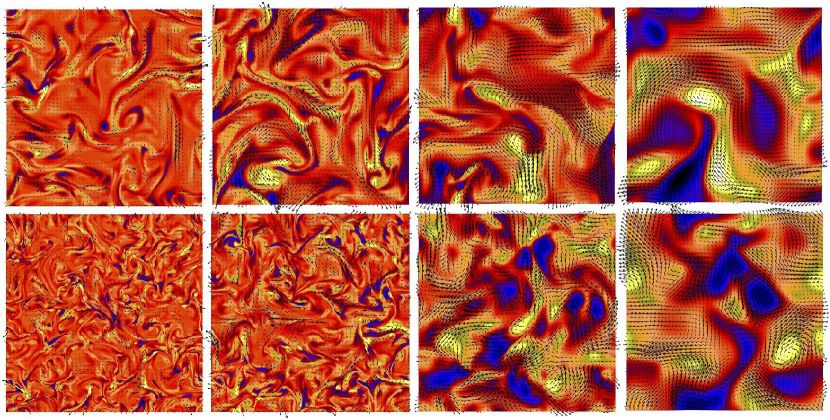
Figure 1: Two-dimensional slices of $B_{z}/B_{\rm rms}$ in the $x-y$ plane from runs B (top row) and D (bottom row), showing the field structure in kinematic (first column), saturated (second column) and decaying phases (last two columns). The fields are strong in blue and yellow regions and negligible in orange regions. The field in the plane of the slices are shown with vectors whose length is proportional to the field strength. For clarity of the color contrast, we have restricted the range of $B_{z}/B_{\rm rms}$ to be $\pm 3.0$ in the kinematic and saturated phase and to $\pm 1.5$ in the decay phases.

3 Results

3.1 Decaying regime in subsonic turbulence

3.1.1 Field structure and time evolution

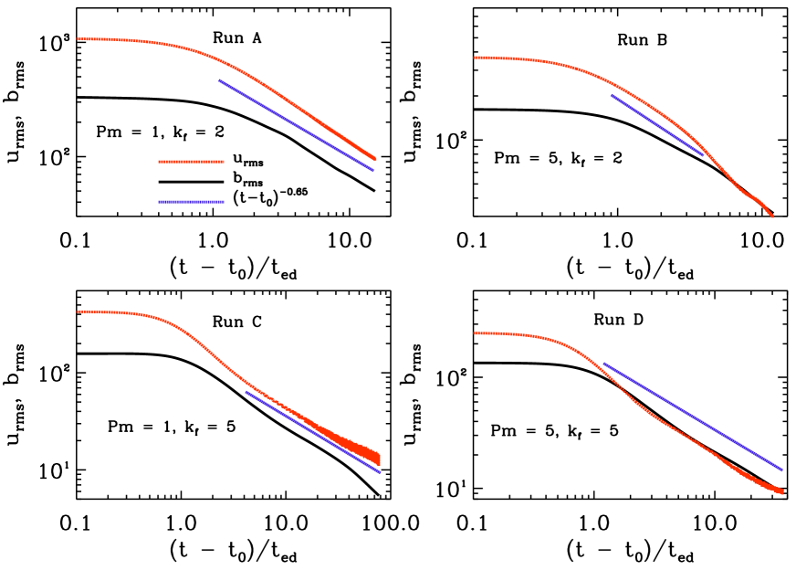
Figure 2: Time evolution of $u_{\rm rms}$ and $b_{\rm rms}$ in the decaying regime as a function of the eddy turnover time. Both variables are normalized in units of ($l_{\rm f}/\nu$), while time is expressed in units of $t^{\prime}=(t-t_{0})/t_{\rm ed}$. The blue dotted lines in each panel shows the $t^{\prime(-0.65)}$ scaling.

In Fig. 1, we show the two-dimensional structure of the magnetic field in kinematic (first column), saturated (second column), and decaying phases (last two columns) for runs B and D. Both these runs have $\rm Pm=5$. However the forcing in run B is at $k_{\rm f}=2$, while it is at $k_{\rm f}=5$ in run D. The slices are in the $x-y$ plane and the $z$-component of the magnetic field normalized to its rms value is shown in color. The field in the plane of the slices are shown with vectors whose length is proportional to the field strength. Because of the presence of only a few turbulent cells, stretching of the magnetic field lines by turbulent eddies is more prominently visible in run B compared to run D (see second column). Field structure at this stage is expected to be highly intermittent having complex internal structure. Once the turbulent forcing is turned off, the intermittency gradually decreases as the field decays together with the turbulence. Structures on smaller scales decay faster and the volume filling factor of the field increases with time. This results in the field structure becoming more homogeneous in both the runs. The magnetic field structures in $\rm Pm=1$ runs (not shown here) also show qualitatively similar features.

Figure 3: The spectra of kinetic (dotted) and magnetic (solid) energies at various stages of evolution, starting from the time turbulent forcing is turned off. In each panel, kinetic and magnetic energies at that time is shown as red dotted and solid lines respectively. The final kinetic and magnetic energy spectra in the decay phase are plotted as thick dotted and thick blue solid lines, respectively. Wavenumber is normalized in units of $k_{\rm min}=2\pi$.

The time evolution of the fluctuation dynamo generated magnetic field in the kinematic stage and all the way up to saturation has been thoroughly studied by a number of authors. Starting from a weak initial seed field, random stretching and folding of the field lines by the turbulent eddies leads to an exponential growth of the magnetic energy eventually saturating at about $10-30$ per cent of the equipartition value (e.g. Haugen et al., 2004; Schekochihin et al., 2004; Brandenburg & Subramanian, 2005; Cho et al., 2009; Federrath et al., 2011; Bhat & Subramanian, 2013; Sur et al., 2018). However as our main objective is to explore the decay of the turbulent velocity and the magnetic field, we show in Fig. 2 the time evolution of the rms velocity ($u_{\rm rms}$) by red dashed lines and the magnetic field ($b_{\rm rms}$) by black solid lines, after the driving was switched off. For clarity in accurately estimating the power-law slopes, we choose to multiply the $u_{\rm rms}$ and $b_{\rm rms}$ by $(l_{\rm f}/\nu)$ while time in the abscissa is represented in units of $t^{\prime}=(t-t_{0})/t_{\rm ed}$, where we use the steady state value of $u_{\rm rms}$ in the estimate of $t_{\rm ed}$. The figure shows that in all the runs both $u_{\rm rms}$ and $b_{\rm rms}$ continue to remain approximately constant for about an eddy-turnover time before eventual decay. The decay of both $u_{\rm rms}$ and $b_{\rm rms}$ can be approximated by $(t-t_{0})^{-0.65}$ power-law scaling (blue dotted line), which is in close agreement with the $-3/5$ scaling obtained from simple analytical estimates (see section 2.2 of Subramanian et al., 2006). The decay of $u_{\rm rms}$ slows down once the velocity reaches the box scale. Note that to achieve $\rm Pm>1$, we have increased the viscosity thereby lowering the Reynolds number. Because of this runs B and D show that the initial decay of $u_{\rm rms}$ is faster than that of $b_{\rm rms}$ before slowing down. In a nutshell, we find that in subsonic turbulence the decay of the rms velocity and the magnetic field is in close agreement with the $-3/5$ power-law scaling and independent of the forcing wave numbers and magnetic Prandtl numbers explored here.

3.1.2 Power Spectra

The evolution of kinetic $K(k)$ and magnetic $M(k)$ energy spectra in the kinematic growth phase and saturated phase of fluctuation dynamos is also known from earlier studies. We therefore focus our discussion only for the decay regime. Fig. 3 shows the temporal evolution of $K(k)$ and $M(k)$ denoted by dotted and solid lines, respectively. To guide the readers, we begin by plotting $K(k)$ and $M(k)$ at a time just before the turbulent forcing is turned off. By then the magnetic field is already saturated. These are denoted by thin dotted red and solid red lines for $K(k)$ and $M(k)$, respectively. Note that in agreement with previous studies (Subramanian et al., 2006; Bhat & Subramanian, 2013; Porter et al., 2015; Sur et al., 2018), $M(k)$ at saturation exceeds $K(k)$ on all but the largest scales. After the forcing is turned off the velocity can still drive turbulent motions on scales where the kinetic energy exceeds the magnetic energy. As shown in Fig. 2 these motions can sustain dynamo action for about an eddy turnover time before terminal decay of turbulence and field sets in.

The overall picture that emerges from Fig. 3 is the following. Both $K(k)$ and $M(k)$ collapses from the high-$k$ end in all the runs. In this phase, run A shows a $\sim k^{-2}$ scaling of both $K(k)$ and $M(k)$ in the range $5<k<15$. Gradually the peak of $K(k)$ shifts to the box scale beyond which the decay is expected to slow down. Similarly $M(k)$ which was peaked around $k\sim 7-9$ in the steady state also approaches the box scale. This implies that the field distribution gradually becomes more homogeneous in agreement with Fig. 1. The spectra at the final time is shown by thick dotted line for $K(k)$ and by thick solid blue line for $M(k)$ in all the panels. Similar behavior is obtained in run B ($\rm Pm=5$) where both $K(k)$ and $M(k)$ also show a $\sim k^{-2}$ scaling during the initial phase of the decay ultimately reaching the box scale. In runs C and D, turbulence was forced at $k_{\rm f}=5$. In the saturated state $M(k)$ peaks at $k\approx 10$ for run C and between $k=10$ and $15$ in run D. In both runs, the spectra shows that at the high-$k$ end both $K(k)$ and $M(k)$ scale as $k^{-3}$ in a narrow range of wave numbers. On the other hand, at the low-$k$ end, $M(k)$ shows a $\sim k^{1.8}$ scaling in both runs during the initial decay which then flattens once the magnetic field is homogenized on the scale of the box.

3.2 Decaying regime in transonic turbulence

We have so far considered the free decay of MHD turbulence in subsonic flows that were artificially driven only by solenoidal modes. Does the decay behavior change when turbulent driving results in transonic flows that are likely to occur in cluster outskirts? Before delving into the results, we first discuss the applicability of driving turbulence purely by solenoidal modes in these regions. Recent cosmological simulations of hierarchical structure formation by Miniati (2015) and Vazza et al. (2017) show that about $50-80$ per cent of the kinetic energy in cluster turbulence is still dominated by solenoidal modes with the contribution from the compressional modes only increasing during merger events. Vazza et al. (2017) further show that while solenoidal turbulence dominates the dissipation of turbulent motions in the central cluster volume at all epochs, dissipation via compressive modes is important at large radii and close to merger events. In the context of our numerical set-up, the above findings suggest that instead of driving turbulence only by solenoidal modes, using a combination of sheared (solenoidal) and compressive forcing is likely to be more closer to reality. To this effect, we make use of the mixed forcing implementation detailed in Federrath et al. (2010, 2011) and report the results obtained from a $512^{3}$ simulation (run E) with ${\rm Re}=\rm Rm\approx 1200$, where the amplitude of the forcing was adjusted such that the steady state $\mathcal{M}\approx 1$. Although the outer correlation scales of gas motions in cluster outskirts are expected to be of the order of the curvature radius of the shocks (which is of order Mpc; Ryu et al., 2008), the eddy turnover time on the outer scale will be larger than on smaller scales. We therefore chose to force turbulence at $k_{\rm f}=5$. Keeping all other conditions the same (i.e. the basic setup, the initial and boundary conditions as described in Sec. 2), we use the mixed forcing implementation of Federrath et al. (2010) where the force field is decomposed into its solenoidal and compressive parts by applying a projection in Fourier space. In index notation, the projection operator can be expressed as $\mathcal{P}^{\zeta}_{ij}({\mbox{\boldmath$k$}{}})=\zeta\,\mathcal{P}^{\perp}_{ij}+(1-\zeta)\,\mathcal{P}^{\parallel}_{ij}$ where $\mathcal{P}^{\perp}_{ij}$ and $\mathcal{P}^{\parallel}_{ij}$ are the solenoidal and compressive projection operators, respectively, and the parameter $\zeta=[0,1]$. Choosing $\zeta=0.2$, we find that at $\mathcal{M}\approx 1$ this results in a solenoidal ratio, i.e. the ratio of the specific kinetic energy in solenoidal modes to the total specific kinetic energy, $\chi_{\rm sol}=e_{\rm sol}/e_{\rm tot}\approx 0.8$, in the saturated phase of the dynamo. This could be due to vorticity generation in interacting shock waves (Sun & Takayama, 2003; Kritsuk et al., 2007; Ryu et al., 2008; Porter et al., 2015).

Figure 4: Same as in Fig. 2, but now for run E with $\mathcal{M}\approx 1,{\rm Pm}=1$.

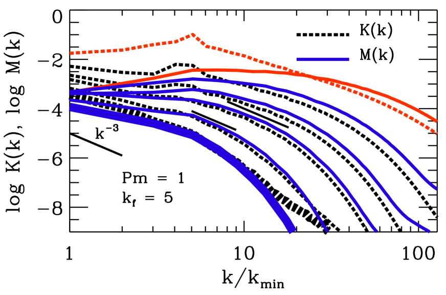
Figure 5: Evolution of $K(k)$ and $M(k)$ in the decay phase for run E starting from the steady state (thin red dashed and red solid lines). Thin black dashed and thin blue solid lines are shown at times $t^{\prime}\approx 10,18,27$ and $55$. The final $K(k)$ and $M(k)$ spectra at $t^{\prime}=112$ are shown by thick dashed black and thick blue solid lines, respectively. Wavenumber is normalized in units of $k_{\rm min}=2\pi$.

Figure 4 shows the evolution of the normalized $u_{\rm rms}$ and $b_{\rm rms}$ from the transonic run. Both the velocity and the magnetic field continue to evolve in steady state for $\approx 2-3\,t_{\rm ed}$ after turbulent forcing has been switched off. Subsequently, during the interval $t^{\prime}=7-20$, both $u_{\rm rms}$ and $b_{\rm rms}$ rapidly decays approximately as $t^{\prime(-1.1)}$. A possible cause for the brisk decrease of $u_{\rm rms}$ could be due to the decay of shocks and shock fronts. Beyond this phase, a change in slope is observed with $u_{\rm rms}$ scaling approximately as $t^{\prime(-0.65)}$ and $b_{\rm rms}$ scaling $\approx t^{\prime(-5/7)}$. The reason for the $t^{\prime(-0.65)}$ scaling of $u_{\rm rms}$ can be understood from the fact that once turbulent driving is turned off, the rms $\mathcal{M}$ also starts to decay. In fact, we find that by $t^{\prime}\sim 20\,t_{\rm ed}$ the rms Mach number decreased by a factor of ten from the steady state value $\mathcal{M}\approx 1$. What follows thereafter is the terminal decay of subsonic motions. Fig. 5 shows time evolution of $K(k)$ and $M(k)$ in the decay phase. As before, the red dashed and red solid lines are the spectra in the non-linear stage just before the turbulent forcing is switched off. Subsequently thin black dashed and blue solid lines depict the spectra of $K(k)$ and $M(k)$, respectively at times $t^{\prime}=10,18,27$ and $55$. Early into the decay, $K(k)$ has a $\sim k^{-3}$ slope in the range $k\sim 8-20$ and thereafter in the range $k\sim 3-6$. The final spectra at $t^{\prime}=112$ are denoted by thick lines.

4 Faraday rotation measure in decaying turbulence

An important observational diagnostic of intracluster magnetic fields is the Faraday rotation of polarized radio emission of background radio sources as seen through the cluster (Clarke et al., 2001; Bonafede et al., 2010, 2013; Govoni et al., 2010, 2017; Han, 2017). This is quantified by the Faraday rotation measure (RM) defined as, ${\rm RM}=K\int_{L}\,n_{\rm e}\mbox{\boldmath$B$}{}\cdot d{\mbox{\boldmath$l$}{}}$. Here $K=0.81\,{\rm rad\,m^{-2}\,cm^{3}\,\,{\rm\mu G}^{-1}\,pc^{-1}}$ is a constant, $n_{\rm e}$ is the thermal electron density measured in ${\rm cm^{-3}}$, $B$ is the magnetic field in $\,{\rm\mu G}$, and the integration is along the line-of-sight (LOS) ’$L$’ (measured in kpc) from the source to the observer. Since the decay of the Faraday RM was already explored for subsonic flows in Subramanian et al. (2006), we limit our analysis here to only transonic flows. Similar to the technique described in Sur et al. (2018), we focus on the decaying phase and compute the RM using $512^{2}$ LOS through the simulation domain along each of the $x,y,$ and $z$ directions of the simulation box. Unlike incompressible flows, we retain $n_{\rm e}$ inside the integral when computing the RM. Since fluctuation dynamo generated fields are expected to be statistically isotropic with $\langle{\rm RM}\rangle=0$ the quantity of interest is the normalized standard deviation of RM, $\bar{\sigma}_{\rm RM}=\sigma_{\rm RM}/\sigma_{\rm RM0}$, where we define the normalization factor for the intracluster gas as

$$\sigma_{\rm RM0} = K\,{\bar{n}_{\rm e}}\frac{b_{\rm rms}}{\sqrt{3}}L\sqrt{\frac{2\pi}{k_{\rm f}L}}\sim 250\,{\rm rad\,m^{-2}}\,\left(\frac{\overline{n}_{\rm e}}{10^{-3}\,{\rm cm^{-3}}}\right)$$ (1)

$$\times\left(\frac{b_{\rm rms}}{2\,{\rm\mu G}}\right)\,\left(\frac{L}{750\,{\rm Mpc}}\right)^{1/2}\,\left(\frac{l_{\rm f}}{100\,{\rm kpc}}\right)^{1/2}.$$

The above factor derives from a simple model of random magnetic fields, where the equipartition fields are assumed to be random with a correlation length $l_{\rm f}=2\pi/k_{\rm f}$. For example, a fluctuation dynamo generated field ordered on the forcing scale is expected to yield $\bar{\sigma}_{\rm RM}\sim 1$. The final value of $\bar{\sigma}_{\rm RM}$ is taken to be the average of the $\bar{\sigma}_{\rm RM}$ values obtained from the estimate of the standard deviations of ${\rm RM}$ along the three LOS. Furthermore, to explore how $\sigma_{\rm RM}$ evolves from steady state as the turbulence decays, we choose to normalize equation (1) using the equipartition value of $b_{\rm rms}$ before turbulent forcing is turned off.

Figure 6: Time evolution of the normalized standard deviation of RM in the decaying phase for the transonic run. The red dotted line shows the $t^{-2/5}$ scaling.

In the subsonic case Subramanian et al. (2006) found that $b_{\rm rms}\propto u_{\rm rms}\propto t^{-3/5}$ and $l_{0}\propto t^{2/5}$, which implies that the observed RM is expected to decrease with time as

$$\bar{\sigma}_{\rm RM}\propto b_{\rm rms}\,l_{0}^{1/2}\propto[(t-t_{0})/t_{\rm ed}]^{-2/5}.$$ (2)

From Fig. 6 we find that for the transonic run the steady state value of $\bar{\sigma}_{\rm RM}\approx 0.56$ similar to what was obtained in Sur et al. (2018). This corresponds to a $\sigma_{\rm RM}\approx 53\,{\rm rad\,m^{-2}}$ (for $\bar{n}_{\rm e}=10^{-4}\,{\rm cm^{-3}},b_{\rm rms}=1\,\,{\rm\mu G}$, path length $L=5\,{\rm Mpc}$, and turbulence forcing scale $l_{\rm f}=800\,{\rm kpc}$), in close agreement with the Faraday RM observed in cluster outskirts (Böhringer et al., 2016). Thereafter, in the decay phase $\bar{\sigma}_{\rm RM}$ scales $\approx t^{-5/7}$; different from the $t^{-2/5}$ scaling (shown by red dotted line) obtained in the subsonic case.

5 Discussion and Conclusions

In this paper, we have explored the free decay of turbulence and magnetic fields in the context of galaxy clusters. The physical picture that forms the basis of our investigation is as follows. We assume that random weak magnetic fields can be amplified to equipartition strengths during the epoch of major mergers. Indeed, as shown by Subramanian et al. (2006) seed fields of $10^{-8}{\rm G}$ strength can be rapidly amplified to $\,{\rm\mu G}$ levels by fluctuation dynamo action assuming that the major merger phase lasts for $\approx 3\,{\rm Gyr}$. After this turbulence is expected to decay resulting in the decay of the magnetic field. Numerically, these two phases composed of turbulent driving and subsequent decay can be simulated using simple idealized simulations. This is the approach that we have followed here. In our simulations, weak seed fields are exponentially amplified by fluctuation dynamo action and then turbulent driving is turned off once the steady state has been captured over sufficient number of eddy turnover times. Keeping in mind that cluster turbulence can be both subsonic (near the centre) and transonic (in the outskirts), we adjusted the amplitude of the driving such that the resulting flows encompass both the above-mentioned regimes.

Consistent with previous works on fluctuation dynamos the field structure is intermittent in the steady state (Haugen et al., 2004; Brandenburg & Subramanian, 2005; Cho et al., 2009; Cho & Ryu, 2009; Bhat & Subramanian, 2013; Porter et al., 2015; Federrath, 2016; Sur et al., 2018). In the saturated state the magnetic spectra exhibit a broad maximum on scales smaller than the forcing scale, while the kinetic energy peaks at the forcing scale. Once the forcing is turned off, we find that both the rms velocity and the magnetic field decays as a power law in time irrespective of whether the turbulent flow in steady state was subsonic or transonic. In cases where the forcing amplitude resulted in subsonic flows the power law exponent in the decay phase is close to the $-3/5$ scaling reported previously (Subramanian et al., 2006). Analysis of the power spectra in Figs 3 and 5 reveals that the decay starts from the high-$k$ end and once the velocity and the magnetic field reaches the box scale the decay slows down. Interestingly, in the transonic case both $u_{\rm rms}$ and $b_{\rm rms}$ initially decay rapidly with time scaling as $t^{\prime(-1.1)}$ (see Fig. 4). We found that this is accompanied by a decreases of the rms Mach number from $\mathcal{M}\approx 1$ to $\sim 0.1$. Beyond this phase, $u_{\rm rms}\sim t^{-0.65}$, while $b_{\rm rms}\sim t^{-5/7}$. A naive estimate from the same figure shows that by $10\,t_{\rm ed}$ (after the turbulent driving is switched off), the rms magnetic field decreased by a factor $\sim 2.25$, while by $50\,t_{\rm ed}$ it has decreased by a factor $\sim 10$. Assuming $l_{\rm f}=100\,{\rm kpc}$ and $u_{\rm rms}=300\,{\rm km\,s^{-1}}$, the eddy turnover time at the forcing scale, $t_{\rm ed}\sim 3\times 10^{8}\,{\rm yr}\approx 0.3\,{\rm Gyr}$. Thus, if the saturated field strength at the end of the merger event was $\sim 1\,\,{\rm\mu G}$, then by $\sim 3\,{\rm Gyr}$ into the decay, $b_{\rm rms}\sim 0.5\,\,{\rm\mu G}$, which would further decrease to $\sim 0.1\,\,{\rm\mu G}$ in about $15\,{\rm Gyr}$. While fluctuation dynamo generated fields were shown to possess significant degree of coherence even in transonic and supersonic flows (Sur et al., 2018), here we applied the analysis to compute the evolution of $\bar{\sigma}_{\rm RM}$ in the decaying phase. In our transonic run, we find that $\bar{\sigma}_{\rm RM}$ also decreases in time as a power law but the decay is $\propto t^{-5/7}$ in comparison to the $\sim t^{-2/5}$ scaling obtained for subsonic runs. While the Faraday RM provides information on the LOS magnetic field, the intensity and polarization of synchrotron emission will provide information on magnetic fields in the sky plane (i.e. perpendicular to the LOS). In a future work, we therefore intend to pursue how the synchrotron intensity and degree of polarization evolves in forced and decaying phases.

Apart from galaxy clusters, another intriguing area where our work can be applied concerns magnetic fields in elliptical galaxies. Because of lack of radio detection of synchrotron emission from the ISM, very little is known about the strength and structure of magnetic fields in these galaxies (Mathews & Brighenti, 1997, 2003), even though the possibility of fluctuation dynamo action cannot be completely ruled out (Moss & Shukurov, 1996). If we assume elliptical galaxies result from mergers of spirals (Barnes, 1992; Naab & Burkert, 2003; Bournaud et al., 2005, 2007; Naab & Ostriker, 2017), the parent spirals may already harbour equipartition strength random magnetic fields resulting from fluctuation dynamo action. Although turbulence is expected to be initially supersonic, it will eventually decay to subsonic levels as these galaxies gradually exhaust their molecular and atomic clouds in earlier star formations. For simplicity, let us assume that equipartition fields are of strengths $\sim 10\,\,{\rm\mu G}$ and that $l_{\rm f}=100\,{\rm pc}$ and $u_{\rm rms}\sim 10\,{\rm km\,s^{-1}}$ implying $t_{\rm ed}\sim 10^{7}\,{\rm yr}$ in the parent spirals. Then our estimates from Fig. 4 suggest that by $100\,t_{\rm ed}\sim 1\,{\rm Gyr}$, the equipartition field strength would be reduced to $\sim 0.5\,{\rm\mu G}$ in elliptical galaxies. In addition to random magnetic fields, spirals also possess large-scale mean magnetic fields ordered on kpc scales. The large scale and the random magnetic fields are generated by different but related physical mechanisms. In the absence of sustained turbulent driving, these helical fields are also expected to decay. While this has been studied for non-helical, subsonic turbulent driving (e.g., Bhat et al., 2014; Brandenburg et al., 2019), a systematic analysis of free decay of helical magnetic fields in transonic and supersonic turbulence still remains to be performed.

References

- Banerjee & Jedamzik (2004) Banerjee R., Jedamzik K., 2004, Phys. Rev. D, 70, 123003
- Barnes (1992) Barnes J. E., 1992, ApJ, 393, 484
- Batchelor & Proudman (1956) Batchelor G. K., Proudman I., 1956, Philosophical Transactions of the Royal Society of London Series A, 248, 369
- Benzi et al. (2008) Benzi R., Biferale L., Fisher R. T., Kadanoff L. P., Lamb D. Q., Toschi F., 2008, Physical Review Letters, 100, 234503
- Bhat & Subramanian (2013) Bhat P., Subramanian K., 2013, MNRAS, 429, 2469
- Bhat et al. (2014) Bhat P., Blackman E. G., Subramanian K., 2014, MNRAS, 438, 2954
- Böhringer et al. (2016) Böhringer H., Chon G., Kronberg P. P., 2016, A&A, 596, A22
- Bonafede et al. (2010) Bonafede A., Feretti L., Murgia M., Govoni F., Giovannini G., Dallacasa D., Dolag K., Taylor G. B., 2010, A&A, 513, A30
- Bonafede et al. (2013) Bonafede A., Vazza F., Brüggen M., Murgia M., Govoni F., Feretti L., Giovannini G., Ogrean G., 2013, MNRAS, 433, 3208
- Bournaud et al. (2005) Bournaud F., Jog C. J., Combes F., 2005, A&A, 437, 69
- Bournaud et al. (2007) Bournaud F., Jog C. J., Combes F., 2007, A&A, 476, 1179
- Brandenburg & Subramanian (2005) Brandenburg A., Subramanian K., 2005, Phys. Rep., 417, 1
- Brandenburg et al. (2015) Brandenburg A., Kahniashvili T., Tevzadze A. G., 2015, Physical Review Letters, 114, 075001
- Brandenburg et al. (2019) Brandenburg A., Kahniashvili T., Mandal S., Pol A. R., Tevzadze A. G., Vachaspati T., 2019, Physical Review Fluids, 4, 024608
- Brandenburg et al. (2017b) Brandenburg A., Kahniashvili T., Mandal S., Pol A. R., Tevzadze A. G., Vachaspati T., 2017b, Phys. Rev. D, 96, 123528
- Brüggen et al. (2005) Brüggen M., Ruszkowski M., Simionescu A., Hoeft M., Dalla Vecchia C., 2005, ApJ, 631, L21
- Cho & Ryu (2009) Cho J., Ryu D., 2009, ApJ, 705, L90
- Cho et al. (2009) Cho J., Vishniac E. T., Beresnyak A., Lazarian A., Ryu D., 2009, ApJ, 693, 1449
- Christensson et al. (2001) Christensson M., Hindmarsh M., Brandenburg A., 2001, Phys. Rev. E, 64, 056405
- Clarke et al. (2001) Clarke T. E., Kronberg P. P., Böhringer H., 2001, ApJ, 547, L111
- Davidson et al. (2012) Davidson P. A., Okamoto N., Kaneda Y., 2012, Journal of Fluid Mechanics, 706, 150
- Dolag et al. (1999) Dolag K., Bartelmann M., Lesch H., 1999, A&A, 348, 351
- Dolag et al. (2002) Dolag K., Bartelmann M., Lesch H., 2002, A&A, 387, 383
- Domínguez-Fernández et al. (2019) Domínguez-Fernández P., Vazza F., Brüggen M., Brunetti G., 2019, MNRAS, 486, 623
- Donnert et al. (2018) Donnert J., Vazza F., Brüggen M., ZuHone J., 2018, Space Sci. Rev., 214, 122
- Eswaran & Pope (1988) Eswaran V., Pope S. B., 1988, Physics of Fluids, 31, 506
- Federrath (2016) Federrath C., 2016, Journal of Plasma Physics, 82, 535820601
- Federrath et al. (2010) Federrath C., Roman-Duval J., Klessen R. S., Schmidt W., Mac Low M. M., 2010, A&A, 512, A81
- Federrath et al. (2011) Federrath C., Chabrier G., Schober J., Banerjee R., Klessen R. S., Schleicher D. R. G., 2011, Physical Review Letters, 107, 114504
- Fryxell et al. (2000) Fryxell B., et al., 2000, ApJS, 131, 273
- Govoni et al. (2010) Govoni F., et al., 2010, A&A, 522, A105
- Govoni et al. (2017) Govoni F., et al., 2017, A&A, 603, A122
- Han (2017) Han J. L., 2017, ARA&A, 55, 111
- Haugen et al. (2004) Haugen N. E., Brandenburg A., Dobler W., 2004, Phys. Rev. E, 70, 016308
- Ishida et al. (2006) Ishida T., Davidson P. A., Kaneda Y., 2006, Journal of Fluid Mechanics, 564, 455
- Kazantsev (1968) Kazantsev A. P., 1968, Soviet Journal of Experimental and Theoretical Physics, 26, 1031
- Kritsuk et al. (2007) Kritsuk A. G., Norman M. L., Padoan P., Wagner R., 2007, ApJ, 665, 416
- Lee (2013) Lee D., 2013, Journal of Computational Physics, 243, 269
- Lee & Deane (2009) Lee D., Deane A. E., 2009, Journal of Computational Physics, 228, 952
- Lesieur & Ossia (2000) Lesieur M., Ossia S., 2000, Journal of Turbulence, 1, 7
- Mac Low et al. (1998) Mac Low M.-M., Klessen R. S., Burkert A., Smith M. D., 1998, Physical Review Letters, 80, 2754
- Marinacci et al. (2015) Marinacci F., Vogelsberger M., Mocz P., Pakmor R., 2015, MNRAS, 453, 3999
- Marinacci et al. (2018) Marinacci F., et al., 2018, MNRAS, 480, 5113
- Mathews & Brighenti (1997) Mathews W. G., Brighenti F., 1997, ApJ, 488, 595
- Mathews & Brighenti (2003) Mathews W. G., Brighenti F., 2003, ARA&A, 41, 191
- Miniati (2014) Miniati F., 2014, ApJ, 782, 21
- Miniati (2015) Miniati F., 2015, ApJ, 800, 60
- Miyoshi & Kusano (2005) Miyoshi T., Kusano K., 2005, Journal of Computational Physics, 208, 315
- Mohapatra & Sharma (2019) Mohapatra R., Sharma P., 2019, MNRAS, 484, 4881
- Moss & Shukurov (1996) Moss D., Shukurov A., 1996, MNRAS, 279, 229
- Mundell et al. (2013) Mundell C. G., et al., 2013, Nature, 504, 119
- Naab & Burkert (2003) Naab T., Burkert A., 2003, ApJ, 597, 893
- Naab & Ostriker (2017) Naab T., Ostriker J. P., 2017, ARA&A, 55, 59
- Paul et al. (2011) Paul S., Iapichino L., Miniati F., Bagchi J., Mannheim K., 2011, ApJ, 726, 17
- Porter et al. (2015) Porter D. H., Jones T. W., Ryu D., 2015, ApJ, 810, 93
- Reppin & Banerjee (2017) Reppin J., Banerjee R., 2017, Phys. Rev. E, 96, 053105
- Roh et al. (2019) Roh S., Ryu D., Kang H., Ha S., Jang H., 2019, arXiv e-prints, p. arXiv:1906.12210
- Ryu et al. (2008) Ryu D., Kang H., Cho J., Das S., 2008, Science, 320, 909
- Saffman (1967) Saffman P. G., 1967, Journal of Fluid Mechanics, 27, 581
- Schekochihin et al. (2004) Schekochihin A. A., Cowley S. C., Taylor S. F., Maron J. L., McWilliams J. C., 2004, ApJ, 612, 276
- Sethi & Subramanian (2005) Sethi S. K., Subramanian K., 2005, MNRAS, 356, 778
- Shi & Zhang (2019) Shi X., Zhang C., 2019, MNRAS, 487, 1072
- Subramanian et al. (2006) Subramanian K., Shukurov A., Haugen N. E. L., 2006, MNRAS, 366, 1437
- Sun & Takayama (2003) Sun M., Takayama K., 2003, Journal of Fluid Mechanics, 478, 237
- Sur et al. (2018) Sur S., Bhat P., Subramanian K., 2018, MNRAS, 475, L72
- Uehara et al. (2012) Uehara T., et al., 2012, ApJ, 752, L6
- Vazza et al. (2017) Vazza F., Jones T. W., Brüggen M., Brunetti G., Gheller C., Porter D., Ryu D., 2017, MNRAS, 464, 210
- Vazza et al. (2018) Vazza F., Brunetti G., Brüggen M., Bonafede A., 2018, MNRAS, 474, 1672
- Zeldovich et al. (1990) Zeldovich Y. B., Ruzmaikin A. A., Sokoloff D. D., 1990, The almighty chance, doi:10.1142/0862.
- Zrake (2014) Zrake J., 2014, ApJ, 794, L26