Hyperon production in $\Lambda_{c}^{+}\to K^{-}p\pi^{+}$ and $\Lambda_{c}^{+}\to K^{0}_{S}p\pi^{0}$

Abstract

We investigate $S=-1$ hyperon production from the $\Lambda_{c}^{+}\to K^{-}p\pi^{+}$ and $\Lambda_{c}^{+}\to K^{0}_{S}p\pi^{0}$ decays within the effective Lagrangian approach. We consider the $\Sigma/\Lambda$ ground states, $\Lambda(1520)$, $\Lambda(1670)(J^{p}=1/2^{-})$, $\Lambda(1890)(J^{p}=3/2^{+})$; $\Lambda/\Sigma$-pole contributions from the combined resonances between 1800 MeV and 2100 MeV; and $N/\Delta$-pole and $K^{\ast}$-pole contributions, which include the proton, $\Delta(1232)$, and $K(892)$. We calculate the Dalitz plot density $(d^{2}\Gamma/dM_{K^{-}p}dM_{K^{-}\pi^{+}}$) for the $\Lambda_{c}^{+}\to K^{-}p\pi^{+}$ decay. The calculated result is in good agreement with experimental data from the Belle Collaboration. Using the parameters from the fit, we present the Dalitz plot density for the $\Lambda_{c}^{+}\to K^{0}_{S}p\pi^{0}$ decay. In our calculation, a sharp peak-like structure near 1665 MeV is predicted in the $\Lambda_{c}^{+}\to K^{-}p\pi^{+}$ decay because of the interference effects between the $\Lambda(1670)$ resonance and $\eta$-$\Lambda$ loop channels. We also demonstrate that we can access direct information regarding the weak couplings of $\Lambda(1670)$ and $\Sigma(1670)$ from the $\Lambda_{c}^{+}\to K^{0}_{S}p\pi^{0}$ decay. Finally, a possible interpretation for the 1665 MeV structure beyond our prediction is briefly discussed.

I Introduction

In the constituent quark model, low-lying baryons with $J^{p}=1/2^{+}$ and $J^{p}=3/2^{+}$ make up the ground-state 56-plet in approximate flavor-spin SU(6) multiplets. Odd-parity baryons are classified into a band with orbital excitation $L=1$, which entails $P=-1$; in combination with $S=1/2$ or $3/2$, this gives negative-parity baryons with $J^{p}=1/2^{-}$, $3/2^{-}$, and $5/2^{-}$. However, the excited states of hyperons are still much less well known compared with the nucleon resonances. Thus, studying hyperon resonances may provide some hints regarding the role of confinement in the nonperturbative QCD region.

In the $S=-1$ sector, only a few states are directly measured in production experiments, whereas other broad states are studied in multichannel particle-wave analyses, mostly with $\overline{K}N$ scattering data. For example, only the $\Lambda(1520)(J^{p}=3/2^{-})$ above the $\overline{K}N$ threshold is reconstructed from its decay channels, $\pi\Sigma$, $\overline{K}N$, and $\pi\pi\Lambda$. Other $\Lambda^{\ast}$ and $\Sigma^{\ast}$ resonances are overlaid with relatively large decay widths so that it is challenging to identify their lineshapes separately from the others in the invariant mass spectra.

In the mass region from 1600 to 2000 MeV, 8 $\Lambda^{\ast}$ and 5 $\Sigma^{\ast}$ resonances are listed in the Particle Data Group (PDG) tables with three- and four-star ratings Tanabashi:2019oca . $\Lambda(1600)(J^{p}=1/2^{+})$ and $\Sigma(1660)(J^{p}=1/2^{+})$ lie below the $\eta\Lambda$ threshold (1663.5 MeV) and are known to have a strong coupling to the $\overline{K}N$, $\pi\Lambda$ and $\pi\Sigma$ channels Gao:2012 . The next $\Lambda(1670)(J^{p}=1/2^{-})$ and $\Sigma(1670)(J^{p}=3/2^{-})$ are very close to the $\eta\Lambda$ threshold. The $\Lambda(1670)$ is interpreted as a resonance strongly coupled to a pure $I=0$ $\eta\Lambda$ state. The nature of the $\Sigma(1670)$ is still poorly known, and the production angular distribution of the $K^{-}p\to\Sigma(1670)^{+}\pi^{-}$ reaction is interpreted as evidence for two mass-degenerate $\Sigma(1670)$ resonances Eberhard:1969 . One couples strongly to $\pi\Sigma$, and the other couples to $\pi\pi\Sigma$. $\Lambda(1690)(J^{p}=3/2^{-})$ decays largely to $\pi\Sigma(1385)$. Above 1700 MeV, another eight $\Lambda^{\ast}$ and $\Sigma^{\ast}$ resonances with three- and four-star ratings appear near each other in the mass range up to 2000 MeV.

A recent observation of hidden-charm pentaquark states reported by the LHCb Collaboration emphasizes the importance of understanding $\Lambda^{\ast}$ and $\Sigma^{\ast}$ resonances in the $K^{-}p$ invariant mass spectrum for $\Lambda_{b}\to J/\psi K^{-}p$ decays LHCb1:2015 ; LHCb2:2019 . In the charm sector, possible evidence for a new $\Lambda^{\ast}$ resonance at a mass of approximately 1665 MeV, just above $\eta\Lambda$ threshold, has been reported from the Belle Collaboration in the $K^{-}p$ invariant mass spectrum for $\Lambda_{c}^{+}\to K^{-}p\pi^{+}$ decays Tanida:2018 . The new $\Lambda^{\ast}$ resonance shows a narrow peak with a Breit-Wigner width of approximately 10 MeV, which could be interpreted as either a dynamically generated $\Lambda(1671)(J^{p}=3/2^{+})$ Kamano:2015hxa , $\Lambda(1667)(J^{p}=3/2^{-})$ in the $D_{03}$ partial wave BChao:2012 , or an exotic $\Lambda^{\ast}$ state. More recently, the peak-like structure was interpreted using the threshold cusp, enhanced by the triangle singularities Liu .

In the $\Lambda^{+}_{c}\to\overline{K}N\pi$, an isospin $I=0$ amplitude of the $\overline{K}N$ system dominates compared with the $I=1$ amplitude because the $\Lambda_{c}^{+}$ is an iso-singlet state and the transition amplitude $c\to su\overline{d}$ has $\Delta I=1$ with $I=1$ pion emission Miyahara:2015cja . Therefore, excited $\Lambda$ hyperons can be selectively produced in the $\overline{K}N$ invariant mass spectrum. Conversely, the large branching fraction of $\Gamma(\Lambda^{+}_{c}\to\Lambda\pi^{0}\pi^{+})/\Gamma_{\rm total}=(7.1\pm 0.4)$% Tanabashi:2019oca ; Ablikim:2017 supports a possible population of excited $\Sigma$ hyperons decaying to $\overline{K}N$, as $\Lambda\pi^{0}$ is a pure $I=1$ state.

Therefore, the $\Lambda^{+}_{c}\to\overline{K}N\pi$ decays are good probes to test the isospin symmetry in non-leptonic decays of the charmed baryon. The $I=1$ $\Sigma^{\ast}$ resonances can only be involved in the $\Lambda_{c}^{+}\to K^{0}_{S}p\pi^{0}$ decays, while the $I=0$ $\Lambda^{\ast}$ resonances are dominant in the $\Lambda_{c}^{+}\to K^{-}p\pi^{+}$ decays. In this respect, it is necessary to conduct measurements of the $\Lambda_{c}^{+}\to K^{0}_{S}p\pi^{0}$ decay. A charged $K^{0}_{S}p$ system ensures a production of $\Sigma^{\ast+}$ hyperons isolated from $\Lambda^{\ast}$ hyperons, thereby providing a good opportunity to test isospin symmetry.

Moreover, a possible interference effect among $\overline{K}N$, $\overline{K}\pi$, and $\pi N$ channels is also very interesting. A strong $K^{\ast}$ band crossing the $\Lambda(1520)$ band shows evidence for interference between $K^{\ast}$ and $\Lambda(1520)$ production channels in the $\Lambda_{c}^{+}\to K^{-}p\pi^{+}$ decay Yang:2015ytm . The phase in the interference between the two resonances can be deduced from experimental data.

In this paper, we report numerical calculation results for $S=-1$ hyperon production from the $\Lambda_{c}^{+}\to K^{-}p\pi^{+}$ and $\Lambda_{c}^{+}\to K^{0}_{S}p\pi^{0}$ decays within the effective Lagrangian approach. We consider the $\Sigma/\Lambda$ ground states, $\Lambda(1520)$, $\Lambda(1670)(J^{p}=1/2^{-})$, $\Lambda(1690)(J^{p}=3/2^{-})$; $\Lambda/\Sigma$-pole contributions from the combined resonances between 1800 MeV and 2100 MeV; and $N/\Delta$-pole and $K^{\ast}$-pole contributions, including the proton, $\Delta(1232)$, and $K(892)$.

We calculate the Dalitz plot density $(d^{2}\Gamma/dM_{K^{-}p}dM_{K^{-}\pi^{+}}$) for the $\Lambda_{c}^{+}\to K^{-}p\pi^{+}$ decay, which is in good agreement with experimental data from the Belle Collaboration. Using the coupling constants from the fit, we present the Dalitz plot density for the $\Lambda_{c}^{+}\to K^{0}_{S}p\pi^{0}$ decay. In our calculation, a sharp resonance-like structure near 1665 MeV is predicted to appear because of the interference effect between $\Lambda(1670)$ production and $\eta$-$\Lambda$ channels. We also demonstrate that we can access direct information regarding weak couplings of $\Lambda(1670)$ and $\Sigma(1670)$ from the $\Lambda_{c}^{+}\to K^{0}_{S}p\pi^{0}$ decay. Finally, a possible interpretation for the 1665 MeV structure beyond our prediction is briefly discussed.

II Theoretical framework

In this Section, we introduce the theoretical framework to study the hadronic $\Lambda^{+}_{c}$ decay within the effective Lagrangian approach. We consider the charged $(\Lambda^{+}_{c}\to\pi^{+}K^{-}p)$ and neutral $(\Lambda^{+}_{c}\to\pi^{0}\overline{K}^{0}p)$ decay channels. Relevant Feynman diagrams for the two channels are illustrated in Fig.  1. The diagrams in Fig. 1($a$), $(b)$, ($c$), ($d)$ denote $Y^{(*)}$-pole, $N/\Delta$-pole, $K^{*}$-pole, and $\eta$-$\Lambda$-loop diagrams, respectively. Although tens of baryon resonances can be accessible from the $\Lambda^{+}_{c}$ decay Tanabashi:2019oca , we take into account only a few resonances to minimize theoretical uncertainties and control numerical calculations.

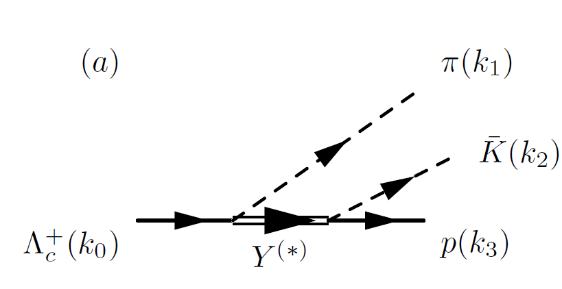
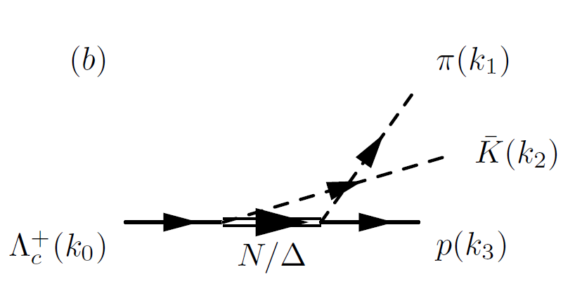
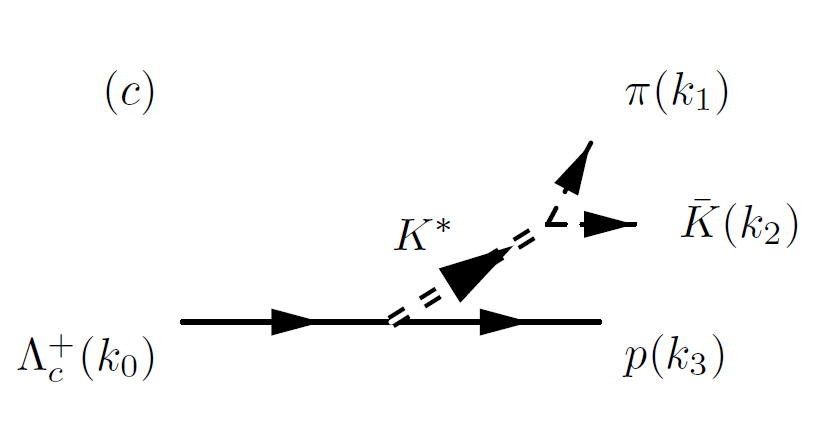
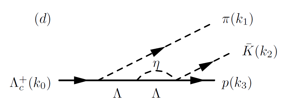
Figure 1: Relevant Feynman diagrams for $\Lambda^{+}_{c}\to\pi\overline{K}p$: ($a$) $Y^{(*)}$-pole diagram, ($b$) $N/\Delta$-pole diagram, ($c$) $K^{*}$-pole diagram, and ($d$) $\eta$-$\Lambda$ loop diagram, where $Y=(\Lambda,\Sigma)$. See the text for details.

Selection criteria for the resonances in the numerical calculations are based on the following points. First, by investigating the Dalitz plot of the Belle experimental data for the charged channel given in Fig. 3 of Ref. Yang:2015ytm (and in Fig 1(a) in the present work), we observe clear signals from $\Lambda(1520)$, $\Lambda(1670)$ (or $\Sigma(1670)$), $\Delta(1232)$, and $K(892)$. Second, there are possible non-resonant backgrounds (BKG) shown in the lower $M^{2}_{K^{-}p}$ region, which can be explained by the ground-state $\Lambda$ and $\Sigma$. Third, excluding $\Delta(1232)$, whose contribution provides a diagonal band in the Dalitz plot, there are no obvious non-strange resonances. This observation can be understood as the color factors of the $u$ and $\overline{d}$ quarks from $W^{+}$ decay are constrained to form the color-singlet pion and resonances. Hence, we only take into account the ground-state nucleon and $\Delta(1232)$. Finally, the authors of Ref. Miyahara:2015cja suggested that, even in the Cabibbo-favored (CF) decays such as those in the diagram ($a$), the isospin $I=1$ hyperon-resonance $(\Sigma^{*})$ contributions are suppressed because of the strong $[ud]$ di-quark correlation inside $\Lambda^{+}_{c}$, whereas the $I=0$ contributions $(\Lambda^{*})$ prevail for the $\Lambda^{+}_{c}$ weak decay with $\pi^{+}$.

		$\Lambda^{+}_{c}\to\pi^{+}K^{-}p$				$\Lambda^{+}_{c}\to\pi^{0}\overline{K}^{0}p$
$B(M,J^{P})$	$\Gamma$ [MeV]	$g_{K^{-}pB}$	$g_{\pi^{+}\Lambda^{+}_{c}B}$	$g_{\pi^{+}pB}$	$g_{K^{-}\Lambda^{+}_{c}B}$	$g_{\overline{K}^{0}pB}$	$g_{\pi^{0}\Lambda^{+}_{c}B}$	$g_{\pi^{0}pB}$	$g_{\overline{K}^{0}\Lambda^{+}_{c}B}$
$p(938,1/2^{+})$	$0$	$-$	$-$	$-$	$-$	$-$	$-$	$13$	$(-7.11,25.90)$
$\Delta(1232,3/2^{+})$	$117$	$-$	$-$	$2.17$	$\underline{0.09}$	$-$	$-$	$1.77$	$\underline{0.09}$
$\Lambda(1116,1/2^{+})$	$0$	$-13.4$	$(-4.6,15.8)$	$-$	$-$	$-$	$-$	$-$	$-$
$\Lambda(1520,3/2^{-})$	$15.6$	$10.92$	$\underline{-0.006}$	$-$	$-$	$-$	$-$	$-$	$-$
$\Lambda(1670,1/2^{-})$	$35$	$1.62$	$\underline{-0.11}$	$-$	$-$	$-$	$-$	$-$	$-$
$\Lambda(1890,3/2^{+})$	$150$	$0.67$	$\underline{0.1}$	$-$	$-$	$-$	$-$	$-$	$-$
$\Sigma(1193,1/2^{+})$	$0$	$4.09$	$(5.4,-2.7)$	$-$	$-$	$5.78$	$(5.4,-2.7)$	$-$	$-$
$K(892,1^{-})$	$50$	$g_{\pi^{+}K^{-}K^{*0}}=3.76$		$g_{K^{*0}p\Lambda^{+}_{c}}=\underline{-0.77}$		$g_{\pi^{0}\overline{K}^{0}K^{*0}}=-2.66$		$g_{K^{*0}p\Lambda^{+}_{c}}=\underline{-0.77}$

Table 1: Relevant inputs for numerical calculations: Full decay widths and strong and weak decay constants for the hadrons involved Sharma:1998rd . The values in parentheses represent the parity violating (PV) and parity conserving (PC) couplings as $(g^{\mathrm{PV}},g^{\mathrm{PC}})$. The weak couplings are in units of $G_{F}V_{ud}V^{*}_{cs}10^{-2}\,\mathrm{GeV}^{2}\approx(1.11\times 10^{-7})$. The underlined values indicate those determined by reproducing the Belle experimental data for $\Lambda^{+}_{c}\to\pi^{+}K^{-}p$ Yang:2015ytm .

Combining these observations and discussions, we can minimize the number of relevant contributions for the $\Lambda^{+}_{c}$ decay into seven and four contributions for the charged and neutral channels, respectively, as shown in Table 1. The table provides the quantum numbers, full widths, and relevant coupling constants. The underlined values in the table indicate those fitted to reproduce the charge-channel data.

There is one caveat: If the $I=0$ $uds$-quark cluster dominates the $\Lambda^{+}_{c}$ hadronic decays together with $\pi^{+}$ in the final state, as suggested in Ref. Miyahara:2015cja , one may expect $\Gamma_{\Lambda^{+}_{c}\to\pi^{+}\Sigma^{0}}/\Gamma_{\Lambda^{+}_{c}\to\pi^{+}\Lambda}\approx 0$, for instance. On the contrary, this decay ratio turns out be almost unity experimentally  Tanabashi:2019oca . Similarly, considering the isospin decompositions of the final state of the $\Lambda^{+}_{c}\to\pi^{+}\overline{K}N$ in the isospin limit, the decay ratio of the neutral and charged channels as in the present work becomes unity because $\mathcal{A}^{(1)}$ disappears in Eq. (35) of Ref. Lu:2016 . However, this is not the case Tanabashi:2019oca , although there can be more complicated contributions, such as the higher-mass hyperon and $\Delta$ resonances, $K^{*}$ contribution, and interferences. Hence, although we have reduced theoretical uncertainties using the $I=0$ meson-baryon channel dominance in the final state Miyahara:2015cja , actual experimental data can exhibit sizable $I=1$ $\Sigma^{*}$-resonance contributions that are different from the present numerical results, which illustrates the future experimental data qualitatively.

Once the relevant contributions are fixed, the effective Lagrangians for the interaction vertices shown in Fig. 1 are defined in general as follows:

$$\mathcal{L}^{\mathrm{weak}}_{PBB} = i(\overline{B}\Gamma_{5}\gamma_{5})P(g^{\mathrm{PV}}_{PBB}-g^{\mathrm{PC}}_{PBB}\gamma_{5})B+\mathrm{h.c.},$$ (1)

$$\mathcal{L}^{\mathrm{weak}}_{PBB^{\prime}} = \frac{i}{M_{P}}(\overline{B}^{\prime}_{\mu}\Gamma_{5})(\partial^{\mu}P)(g^{\mathrm{PV}}_{PBB^{\prime}}-g^{\mathrm{PC}}_{PBB^{\prime}}\gamma_{5})B+\mathrm{h.c.},$$ (2)

$$\mathcal{L}^{\mathrm{strong}}_{PBB} = -ig_{PBB}(\overline{B}\Gamma_{5})PB+\mathrm{h.c.},$$ (3)

$$\mathcal{L}^{\mathrm{strong}}_{PBB^{\prime}} = -\frac{ig_{PBB^{\prime}}}{M_{P}}(\overline{B}^{\prime}_{\mu}\Gamma_{5}\gamma_{5})(\partial^{\mu}P)B+\mathrm{h.c.},$$ (4)

$$\mathcal{L}_{VBB} = g_{VN\Lambda_{c}}\overline{B}\not{V}\gamma_{5}(g^{\mathrm{PV}}_{VBB}-g^{\mathrm{PC}}_{VBB}\gamma_{5})B+\mathrm{h.c.},$$ (5)

$$\mathcal{L}_{PPV} = ig_{PPV}V_{\mu}\left[P\partial^{\mu}P^{\dagger}-P^{\dagger}\partial^{\mu}P\right]+\mathrm{h.c.},$$ (6)

where $P$, $B$, $B^{\prime}$, and $V$ represent the $0^{-}$ pseudoscalar meson, $1/2^{\pm}$ baryon, $3/2^{\pm}$ baryon, and $1^{-}$ vector meson, respectively. $\Gamma_{5}$ defines the parity for the created baryon ($\overline{B}$) by

$$\Gamma_{5}=\Big{\{}\begin{array}[]{c}\gamma_{5}\,\,\,\mathrm{for}\,\,\,1/2^{+},\,3/2^{+},\\ 1_{4\times 4}\,\,\,\mathrm{for}\,\,\,1/2^{-},\,3/2^{-}.\end{array}$$ (7)

In principle, the PC and PV vertices have different coupling strengths. Note that Ref. Sharma:1998rd , using the heavy-quark effective field theory (HQEFT), provides the PC and PV weak couplings for $\Lambda^{+}_{c}$ decays into octet hadrons. For instance, $g^{\mathrm{PV}}_{\pi^{+}\Lambda\Lambda^{+}_{c}}=-4.6$ and $g^{\mathrm{PC}}_{\pi^{+}\Lambda\Lambda^{+}_{c}}=15.8$ in units of $G_{F}V_{ud}V^{*}_{cs}10^{-2}\mathrm{GeV}^{2}$. Here, $G_{F}$ and $V_{ud,cs}$ indicate the Fermi constant and CKM matrix elements, respectively. However, regarding $\Lambda^{+}_{c}$ decays into hyperon resonances, there is little experimental or theoretical information from which to extract relevant PC and PV weak couplings. Hence, to reduce theoretical uncertainties, we assume that $g^{\mathrm{PC}}_{PY^{*}\Lambda^{+}_{c}}=g^{\mathrm{PV}}_{PY^{*}\Lambda^{+}_{c}}=g_{PY^{*}\Lambda^{+}_{c}}$ for the hyperon resonances and determine the value of $g_{PY^{*}\Lambda^{+}_{c}}$ using the experimental data, as described previously.

The invariant amplitudes for the diagrams in Fig. 1 can be computed straightforwardly using the effective Lagrangians defined above. The total invariant amplitude is as follows:

$$i\mathcal{M}^{(a)}_{B} = ig_{KNB}\frac{\overline{u}_{p}\Gamma_{5}\Delta(q_{2+3})\Gamma_{5}\gamma_{5}(g^{\mathrm{PV}}_{\pi B\Lambda_{c}}-g^{\mathrm{PC}}_{\pi B\Lambda_{c}}\gamma_{5})u_{\Lambda^{+}_{c}}}{q^{2}_{2+3}-M^{2}_{B}-i\Gamma_{B}M_{B}},$$ (8)

$$i\mathcal{M}_{B^{\prime}}^{(a)} = -\frac{ig_{KNB^{\prime}}}{M_{K}M_{\pi}}\frac{\overline{u}_{p}\gamma_{5}\Gamma_{5}[\Delta_{\mu\nu}(q_{2+3})k^{\mu}_{2}k^{\nu}_{1}]\Gamma_{5}(g^{\mathrm{PV}}_{\pi B^{\prime}\Lambda_{c}}-g^{\mathrm{PC}}_{\pi B^{\prime}\Lambda_{c}}\gamma_{5})u_{\Lambda^{+}_{c}}}{q^{2}_{2+3}-M^{2}_{B^{\prime}}-i\Gamma_{B^{\prime}}M_{B^{\prime}}},$$ (9)

$$i\mathcal{M}^{(b)}_{B} = ig_{\pi NB}\frac{\overline{u}_{p}\Gamma_{5}\Delta(q_{1+3})\Gamma_{5}\gamma_{5}(g^{\mathrm{PV}}_{KB\Lambda_{c}}-g^{\mathrm{PC}}_{KB\Lambda_{c}}\gamma_{5})u_{\Lambda^{+}_{c}}}{q^{2}_{1+3}-M^{2}_{B}-i\Gamma_{B}M_{B}},$$ (10)

$$i\mathcal{M}_{B^{\prime}}^{(b)} = -\frac{ig_{\pi NB^{\prime}}}{M_{K}M_{\pi}}\frac{\overline{u}_{p}\gamma_{5}\Gamma_{5}[\Delta_{\mu\nu}(q_{1+3})k^{\mu}_{1}k^{\nu}_{2}]\Gamma_{5}(g^{\mathrm{PV}}_{KB^{\prime}\Lambda_{c}}-g^{\mathrm{PC}}_{KB^{\prime}\Lambda_{c}}\gamma_{5})u_{\Lambda^{+}_{c}}}{q^{2}_{1+3}-M^{2}_{B^{\prime}}-i\Gamma_{B^{\prime}}M_{B^{\prime}}},$$ (11)

$$i\mathcal{M}^{(c)}_{V} = ig_{\pi KV}\frac{\overline{u}_{p}\left[\not{q}_{1-2}-\not{q}_{1+2}(M^{2}_{\pi}-M^{2}_{K})/M^{2}_{V}\right]\gamma_{5}(g^{\mathrm{PV}}_{VN\Lambda_{c}}-g^{\mathrm{PC}}_{VN\Lambda_{c}}\gamma_{5})u_{\Lambda^{+}_{c}}}{M^{2}_{12}-M^{2}_{V}-i\Gamma_{V}M_{V}},$$ (12)

where the propagators for the spin-$1/2$ and spin-$3/2$ baryons are defined by

$$\Delta(q)=(\not{q}+M_{B}),$$

$$\Delta_{\mu\nu}(q)=(\not{q}+M_{B}) \Bigl{[}g_{\mu\nu}-\frac{1}{3}\gamma_{\mu}\gamma_{\nu}-\frac{1}{3M_{B}}(\gamma_{\mu}q_{\nu}-\gamma_{\nu}q_{\mu})$$ (13)

$$-\frac{2}{3M^{2}_{B}}q_{\mu}q_{\nu}\Bigr{]}.$$

Now, the resonance-band patterns on the Dalitz plot are discussed in detail, as these patterns indicate nontrivial interferences between the resonance contributions and additional contributions. By carefully examining the $\Lambda(1670)$ band at $M^{2}_{K^{-}p}\approx 2.79\,\mathrm{GeV}^{2}$ in the Dalitz plot given in Fig. 1(a), quite different patterns are observed between the left and right sides of the $K^{*}$ band. Moreover, the $K^{*}$ band exhibits a nontrivial pattern as well, i.e., it is distorted in the region where interference with the $\Lambda(1670)$ band occurs. To interpret this complicated pattern in the $\Lambda(1670)$-$K^{*}$ interference region, we consider the $\eta$-$\Lambda$ loop in a simple model; the loop channel opens at $(M_{\eta}+M_{\Lambda})^{2}=2.767\,\mathrm{GeV}^{2}$, and it can cause complicated structures, such as a cusp Bugg:2008wu . The relevant Feynman diagram for describing the $\eta$-$\Lambda$ loop is depicted in Fig 1(d). This simple diagram is important for the following reasons. First, all the vertex structures are theoretically known, i.e., the weak $\pi\Lambda\Lambda^{+}_{c}$ and strong $\eta\Lambda\Lambda$ vertices are given by HQEFT Sharma:1998rd and the Nijmegen soft-core potential Rijken:2010zzb as shown in Eq. (1). The $\eta\overline{K}p\Lambda$ vertex is characterized by the Weinberg-Tomozawa (WT) chiral interaction:

$$\mathcal{L}_{\Phi\Phi^{\prime}BB^{\prime}}=-\frac{ig_{\Phi\Phi^{\prime}BB^{\prime}}}{4f^{2}_{\Phi}}\overline{B}(\Phi^{\prime}\not{\partial}\Phi-\Phi\not{\partial}\Phi^{\prime})B,$$ (14)

where $\Phi$ and $B$ denote the octet pseudo-scalar meson and baryon, respectively. Explicitly for the diagram given in Fig. 1(d), we use $g_{K^{-}p\eta\Lambda}=3/2$ Hyodo:2011ur , $g_{\eta\Lambda\Lambda}=-6.86$ Hyodo:2011ur , and $f_{\Phi}=f_{\pi}\times 1.123\approx 105$ MeV Miyahara:2015cja for numerical calculations. Second, as discussed in Ref. Miyahara:2015cja , the $I=1$ meson-baryon channel is suppressed similar to the $\eta$-$\Sigma^{0}$ one, in terms of the strong di-quark configuration inside $\Lambda^{+}_{c}$.

Using the relevant interaction Lagrangians for the vertices in Eqs. (1) and (14), the diagram with a meson-baryon loop is computed as follows:

$$i\mathcal{M}_{\eta\Lambda} = -\frac{g_{K^{-}p\eta\Lambda}\,g_{\eta\Lambda\Lambda}\theta_{\eta\Lambda}}{4f^{2}_{\Phi}}\int\frac{d^{4}q}{(2\pi)^{4}}\left[\frac{\overline{u}_{p}(\not{q}+\not{k}_{3})(\not{q}_{2+3}-\not{q}+M_{\Lambda})\gamma_{5}(\not{q}_{2+3}+M_{\Lambda})(g^{\mathrm{PV}}_{\pi^{+}\Lambda\Lambda^{+}_{c}}-\gamma_{5}g^{\mathrm{PC}}_{\pi^{+}\Lambda\Lambda^{+}_{c}})u_{\Lambda^{+}_{c}}}{[q^{2}-M^{2}_{\eta}][(q-q_{2+3})^{2}-M^{2}_{\Lambda}][q_{2+3}^{2}-M^{2}_{\Lambda}]}\right]$$ (15)

$$\approx \frac{ig_{K^{-}p\eta\Lambda}\,g_{\eta\Lambda\Lambda}\theta_{\eta\Lambda}}{4f^{2}_{\Phi}}\,G(q^{2}_{2+3})\,\frac{\overline{u}_{p}(\not{q}_{2+3}+\not{k}_{3}-M_{\Lambda})\gamma_{5}(\not{q}_{2+3}+M_{\Lambda})(g^{\mathrm{PV}}_{\pi^{+}\Lambda\Lambda^{+}_{c}}-\gamma_{5}g^{\mathrm{PC}}_{\pi^{+}\Lambda\Lambda^{+}_{c}})u_{\Lambda^{+}_{c}}}{[q_{2+3}^{2}-M^{2}_{\Lambda}]},$$ (16)

where $q_{i+j}\equiv k_{i}+k_{j}$, The step function for the $\eta$-$\Lambda$ channel threshold is defined by $\theta_{\eta\Lambda}=\theta(M_{\overline{K}p}-M_{\eta}-M_{\Lambda})$. In deriving the $\eta$-$\Lambda$ loop integral in Eq. (15), the on-shell factorization Hyodo:2011ur is employed, which assumes that $\Lambda$ in the loop is almost its on-shell. This approximately satisfies the following relationship:

$$(\not{q}_{2+3}-\not{q})u_{\Lambda}\approx M_{\Lambda}u_{\Lambda}\to\not{q}\approx(\not{q}_{2+3}-M_{\Lambda}).$$ (17)

The loop divergence is regularized by the dimensional regularization and the meson-baryon propagating function $G$ is given by Nam:2003ch

$$G_{\mathrm{dim}}(q^{2}_{2+3}) = i\int\frac{d^{4}q}{(2\pi)^{4}}\frac{2M_{\Lambda}}{[q^{2}-M^{2}_{\eta}][(q-q_{2+3})^{2}-M^{2}_{\Lambda}]}$$ (18)

$$= \frac{2M_{\Lambda}}{16\pi^{2}}\left[\frac{M^{2}_{\eta}-M^{2}_{\Lambda}+q^{2}_{2+3}}{2q^{2}_{2+3}}\ln\frac{M^{2}_{\eta}}{M^{2}_{\Lambda}}+\frac{\xi}{2q^{2}_{2+3}}\ln\frac{M^{2}_{\eta}+M^{2}_{\Lambda}-q^{2}_{2+3}-\xi}{M^{2}_{\eta}+M^{2}_{\Lambda}-q^{2}_{2+3}+\xi}\right]+\frac{2M_{\Lambda}}{16\pi^{2}}\ln\frac{M^{2}_{\Lambda}}{\mu^{2}},$$ (19)

where $\xi$ is defined by

$$\xi\equiv\sqrt{[q^{2}_{2+3}-(M^{2}_{\eta}-M^{2}_{\Lambda})^{2}][q^{2}_{2+3}-(M^{2}_{\eta}+M^{2}_{\Lambda})^{2}]}.$$ (20)

The subtraction scale for the regularization is chosen as $\mu=630$ MeV, which is responsible for dynamically reproducing the $S=-1$ hyperon resonances in the couple-channel chiral-unitary model (ChUM) Hyodo:2011ur .

The total amplitude consists of the relevant contributions as follows:

$$i\mathcal{M}_{\mathrm{total}} = i\sum_{\Lambda^{*}}c_{\Lambda^{*}}\mathcal{M}_{\Lambda^{*}}F_{\Lambda^{*}}+ic_{\Lambda}\mathcal{M}_{\Lambda}F_{\Lambda}+ic_{\Sigma}\mathcal{M}_{\Sigma}F_{\Sigma}$$ (21)

$$+ ic_{N}\mathcal{M}_{N}F_{N}+ic_{\Delta}\mathcal{M}_{\Delta}F_{\Delta}+ic_{K^{*}}\mathcal{M}_{K^{*}}F_{K^{*}}$$

$$+ ic_{\eta{\textrm{-}}\Lambda}\mathcal{M}_{\eta{\textrm{-}}\Lambda}F_{\eta{\textrm{-}}\Lambda},$$

where the coefficients $c_{h}$ and $F_{h}$ denote the relative phase factor and phenomenological form factor for the hadron $h$, respectively. Note that the $\Lambda^{*}$ ($N$) contribution is only given in the charged (neutral) channel. The phenomenological form factors are considered because the hadrons are spatially extended objects. In the present work, we employ the following parameterization:

$$F_{h}(q^{2}_{h})=\frac{\mathcal{C}\Lambda^{4}}{\Lambda^{4}+(q^{2}_{h}-M^{2}_{h})},$$ (22)

where $q_{h}$ and $M_{h}$ denote the momentum transfer and mass of the intermediate hadron, respectively. For brevity, we fix the cutoff mass $\Lambda=1.0$ GeV for all hadrons throughout the present work. To compensate for this simplification regarding the cutoff choices, we introduce a phenomenological parameter $\mathcal{C}$ in Eq. (22), which will be adjusted to reproduce the decay width of the experimental data.

III Numerical results and Discussions

In this Section, we discuss the numerical results for the $\Lambda_{c}^{+}$ decays. We first show the numerical results for the Dalitz plots for the charged ($\Lambda^{+}_{c}\to\pi^{+}K^{-}p$) and neutral ($\Lambda^{+}_{c}\to\pi^{0}\overline{K}^{0}p$) channels in Fig. 2. According to the calculated Dalitz plot density, simulated events are generated over the phase space available. We assume a uniform experimental acceptance for the $\pi\overline{K}p$ phase space. Note that all unknown weak coupling constants and phase factors in Eq. (21) are carefully determined to reproduce the data, focusing on the complicated interference patterns in the Dalitz plot of the Belle data Yang:2015ytm , as listed in Table 1 and 2. To determine the phenomenological parameter for the form factor in Eq. (22), which will provide the overall strength of the decay width, we employ the experimental data for the decay ratio between the charged and neutral channels. Considering that the $\Lambda^{+}_{c}(2286,1/2^{+})$ baryon has a life time of $\tau_{\Lambda^{+}_{c}}=(2\times 10^{-13})$ s, which corresponds to $\Gamma_{\Lambda^{+}_{c}}=(3.29\times 10^{-9})$ MeV Tanabashi:2019oca and employing the PDG values of the partial decay ratios for the charge and neutral decays, the resulting relationship is

$$\Gamma_{\Lambda^{+}_{c}\to\pi^{+}K^{-}p} = (2.09\times 10^{-10})\,\mathrm{MeV},~{}~{}~{}~{}~{}~{}$$

$$\Gamma_{\Lambda^{+}_{c}\to\pi^{0}\overline{K}^{0}p} = (1.31\times 10^{-10})\,\mathrm{MeV}.$$ (23)

We note that $\overline{K}^{0}$ is a mixture of $K^{0}_{S}$ and $K^{0}_{L}$ in the same proportion, if we ignore the CP violation. Furthermore, in general, in the experimental data, the $K^{0}_{S}$ was measured for the $\Lambda^{+}_{c}$ decay, as shown in Tanabashi:2019oca . Thus, we simply doubled the experimental partial-decay ratio in our theoretical calculations, as shown in Eq. (III). To reproduce these decay widths, we choose $\mathcal{C}_{\mathrm{charged}}=5.25$ and $\mathcal{C}_{\mathrm{neutral}}=3.15$ in Eq. (22).

	$c_{h}$		$c_{h}$
$p(939)$	$-0.9i$	$\Delta(1232)$	1
$\Lambda(1116)$	$-0.9i$	$\Sigma(1193)$	$-0.9i$
$\Lambda^{*}(1520)$	1	$K^{*}(892)$	$i$
$\Lambda^{*}(1670)$	1	$\eta$-$\Lambda$	$1.8i$
$\Lambda^{*}(1890)$	1

Table 2: Relative phase factors for the amplitudes in Eq. (21). Note that the phase factor for the $\eta$-$\Lambda$ loop contribution is also introduced.

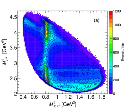
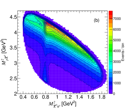
Figure 2: (Color online) Dalitz plots for (a) $\Lambda^{+}_{c}\to\pi^{+}K^{-}p$ for $\Lambda^{+}_{c}\to\pi^{+}K^{-}p$ and (b) $\Lambda^{+}_{c}\to\pi^{0}\overline{K}^{0}p$.

As clearly shown in Fig 2(a), the contributions from $\Lambda(1520)$ and $\Lambda(1670)$, as the horizontal bands, are consistent with the data. We also note that the small contribution from $\Lambda(1890)$ increases the strength of the $K^{*}$ band in the interference region. The $\Delta(1232)$ contribution provides the sloped band in the upper region of the Dalitz plots. The nontrivial pattern shown in the $K^{*}$-$\Lambda(1670)$ interference region is qualitatively reproduced by the $\eta$-$\Lambda$ loop. We verified that the $\Lambda(1670)$ band becomes smooth and shows no complicated interference patterns without the $\eta$-$\Lambda$ loop. From this observation, we conclude that the nontrivial interference patterns in the region of interest are due to the $\eta$-$\Lambda$ loop and nontrivial phase factors given in Table 2. Moreover, this observation indicates that the coherent sum using Breit-Wigner amplitudes does not accurately represent reality.

Once all the couplings are considered, including the phase factors shown in Tables 1 and 2, we attempt to predict the neutral channel, i.e., $\Lambda^{+}_{c}\to\pi^{0}\overline{K}^{0}p$, which has not yet been reported experimentally. Note that we choose the same phase factor $-0.9i$ for the proton as for the $\Lambda$ and $\Sigma$ BKGs. The numerical result for the Dalitz plot is depicted in Fig. 2(b). Because there are no $I=0$ hyperon resonances in this channel, we observe dominant contributions from the $K(892)$, $\Delta(1232)$, and $p$, in addition to the small ground-state $\Sigma$ background. Note the lack of an $I=0$ channel opening effect here.

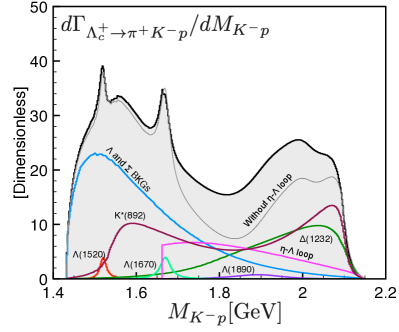
r1.cmt0.5cm(a) r1.cmt0.5cm(b)

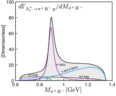
Figure 3: (Color online) Invariant-mass distributions for the charged channel as functions of (a) $M_{K^{-}p}$ and (b) $M_{\pi^{+}K^{-}}$.

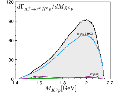
r1.cmt0.5cm(a) r1.cmt0.5cm(b)

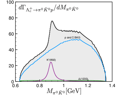
Figure 4: (Color online) Invariant-mass distributions for the neutral channel as functions of (a) $M_{\overline{K}^{0}p}$ and (b)$M_{\pi^{0}\overline{K}^{0}}$.

With these data, it is possible to investigate the invariant-mass distributions. In Figs. 3(a) and (b), we draw their numerical results as functions of $M_{K^{-}p}$ and $M_{\pi^{+}K^{-}}$, respectively, for the charged channel. The curves for each contribution are also shown to highlight their complicated combination for the distribution. As shown in Fig. 3(a), peaks for the $\Lambda(1520)$ and $\Lambda(1670)$ contributions are easily observed. The two bumps are generated by the $K(892)$ contribution at $M_{K^{-}p}\approx 1.6$ GeV and $2.1$ GeV, whereas the ground-state $\Lambda$ and $\Sigma$ BKGs dominate the low-invariant-mass region. Interestingly, because of the interference between the $\eta$-$\Lambda$ loop and $\Lambda(1670)$, a peak-like sharp structure appears in the vicinity of $M_{K^{-}p}\approx 1.67$ GeV. Notably, this peak-like structure is inevitable when reproducing the nontrivial interference pattern observed in the charged-channel Dalitz plot from the experimental data. In Fig. 3(b), the distribution as a function of $M_{\pi^{+}K^{-}}$, the $K(892)$ dominates in addition to the considerable contributions from the hyperon BKGs and $\Delta$, while the $\eta$-$\Lambda$ loop contribution is not obvious.

Similarly, Figs. 4(a) and (b) provide the numerical results for the invariant-mass distributions for the neutral channel, i.e., $\Lambda^{+}_{c}\to\pi^{0}\overline{K}^{0}p$, which has not yet been reported experimentally. As shown in Fig. 4(a), considering the $I=1$ channel suppression, DCS Miyahara:2015cja , and absence of $I=0$ hyperons, the distribution as a function of $M_{\overline{K}^{0}p}$ does not show peak-like structures at all. Instead, the proton-pole contribution dominates the distribution and provides a large bump structure at $M_{\overline{K}^{0}p}\approx 2$ GeV, whereas the ground-state $\Sigma$, $\Delta(1232)$, and $K(892)$ contributions are small. In Fig. 4(b), we show the distribution as a function of $M_{\pi^{0}\overline{K}^{0}}$. We observe a clear peak generated from the $K(892)$ contribution on top of the $p$-pole contribution.

Finally, an important aspect of the results is the considerably narrow band structure at $M_{K^{-}p}\approx 1.67$ GeV, as shown in the Dalitz plot in Fig. 4(a). Compared with the width of $\Lambda(1520)$, the band width is similar to that of $\Gamma_{\Lambda(1520)}\approx 15$ MeV. There are several possibilities to explain the narrow band. First, there have thus far been no such hyperon resonances with such a narrow width at $M_{Y^{*}}=(1.6\sim 1.7)$ GeV Tanabashi:2019oca . Given this observation, the band might signal a missing hyperon resonance, as reported in Ref. Kamano:2015hxa , i.e., $\Lambda(1671)(J^{p}=3/2^{+})$ with a width of $\Gamma\approx 10$ MeV. However, we verified that it is difficult to reproduce the nontrivial interference pattern by combining the two Breit-Wigner-type amplitudes, i.e., the new hyperon resonance and $K(892)$ contributions. Second, there are complicated interferences between the known hyperon resonances at $M_{\overline{K}p}=(1.6\sim 1.7)$ GeV, such as $\Lambda(1600)$, $\Lambda(1670)$, $\Lambda(1690)$. However, we verified that it is almost impossible to form this peak structure numerically. Third, the interference between the $\Lambda(1670)$ and $\eta$-$\Lambda$ loop channels has been explored in this work and the nontrivial interference pattern and narrow peak-like structure have been qualitatively explained. However, as discussed in Section II, theoretical considerations simplify the interpretation; for example, the strong di-quark correlation inside $\Lambda^{+}_{c}$ and color-factor for the non-strange resonances provide constraints.

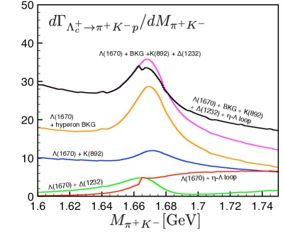
Figure 5: (Color online) The interference patterns between $\Lambda(1670)$ and other contributions. See the text for details.

The interference effects between the $\Lambda(1670)$ and other channels are illustrated in the vicinity of $M_{K^{-}p}\approx 1.67$ GeV in Fig. 5. It is obvious that the $\Delta(1232)$, $K(892)$, and hyperon BKG channels enhance the $\Lambda(1670)$ structure and result in a large peak at 1.67 GeV. On the other hand, A strong destructive interference effect between the $\Lambda(1670)$ and $\eta$-$\Lambda$ loop channels is observed and provides the sharp peak-like structure near the $\eta$-$\Lambda$ threshold.

IV Summary

In this study, we investigated the excited hyperon production in the $\Lambda^{+}_{c}\to\pi^{+}K^{-}p$ (charged) and $\Lambda^{+}_{c}\to\pi^{0}\overline{K}^{0}p$ (neutral) decays within the effective Lagrangian approach. We determined relevant model parameters for phenomenological form factors at the tree-level Born approximation based on experimental data for $\Lambda^{+}_{c}\to\pi^{+}K^{-}p$ Yang:2015ytm and the known decay branching ratios for $\Lambda^{+}_{c}$  Tanabashi:2019oca . We list important observations as follows:

• To reduce the number of hyperons considered, we accounted for the strong di-quark correlation inside $\Lambda^{+}_{c}$ and color-factor constraint of the quarks from $W^{+}$, which makes it possible to drop the $\Sigma^{*}$, $\Delta^{*}$, and $N^{*}$ contributions in the numerical calculations, although there seem non-negligible $I=0$ contributions in reality. As a result of these assumptions, the theoretical uncertainties were substantially diminished.

• Regarding the charged-channel decay, on top of the hyperon backgrounds, $\Lambda(1520)$ and $\Lambda(1670)$ exhibited obvious peaks in the invariant-mass distribution in addition to the bump structure, caused by the interference between the $\Delta(1232)$ and $K(892)$. The Belle experimental data for the Dalitz plot are qualitatively reproduced.

• A nontrivial interference pattern was observed in the charged-channel Dalitz plot at the interference region between $\Lambda(1670)$ and $K(892)$, which can be explained successfully by including the $\eta$-$\Lambda$ loop contribution. Moreover, this complicated interference generates the peak-like structure at $M_{K^{-}p}\approx 1.655$ MeV.

• Given the previous point, we did not observe a sharp peak (band) structure in the neutral channel, as the $I=0$ meson-baryon channel opening was absent. By contrast, a sharp peak-like structure, together with a nontrivial interference pattern in experiments, indicate a small but finite $I=1$ channel opening is possible as a next-to-leading contribution to the di-quark configuration of $\Lambda^{+}_{c}$.

• Regarding the neutral channel with the model parameters, determined by the charged-channel data and theory models, a strong background from the proton-pole contribution was observed. The result was an absence of clear peak-like structures in the invariant-mass distribution as a function of $M_{\overline{K}^{0}p}$, while the $K(892)$ contribution showed an obvious peak on top of the proton background in the invariant-mass distribution as a function of $M_{\pi^{0}\overline{K}^{0}}$.

As discussed, the charmed-baryon decays are good places to study weak interactions in the context of Cabibbo-favored decays, isospin selections, and confinement corresponding to the color factor of $W^{+}$ decays. Moreover, the internal structure of the involved hadrons can be probed by comparing the di-quark scenario with experiments. The channel-opening effects are clearly also important. Therefore, the charmed-baryon decay with $S=0$ hadrons is an interesting alternative to understanding weak and strong interactions. Related studies are in progress and will appear elsewhere.

- (1) M. Tanabashi et al. [Particle Data Group], Phys. Rev. D 98, 030001 (2018).
- (2) P. Gao, J. Shi and B. S. Zou, Phys. Rev. C 86, 025201 (2012).
- (3) P. Eberhard, J. H. Friedman, M. Pripstein and R. R. Ross, Phys. Rev. Lett. 22, 200 (1969).
- (4) T. Skwarnicki on behalf of the LHCb Collaboration, Hadron spectroscopy and exotic states at LHCb, talk given at Moriond QCD 2019, http://moriond.in2p3.fr/2019/QCD/Program.html.
- (5) R. Aaij et al. (LHCb Collaboration), Phys. Rev. Lett. 115, 072001 (2015).
- (6) K. Tanida on behalf of Belle Collaboration, Possibility of a new narrow resonance near the threshold, talk given at HYP2018.
- (7) H. Kamano, S. X. Nakamura, T.-S. H. Lee and T. Sato, Phys. Rev. C 92, no. 2, 025205 (2015) Erratum: [Phys. Rev. C 95, no. 4, 049903 (2017)].
- (8) B. Chao and J.-J. Xie, Phys. Rev. C 85, 055202 (2012).
- (9) X.-H. Liu, G. Li, J.-J. Xie and Q. Zhao, arXiv:1906.07942 (2019).
- (10) K. Miyahara, T. Hyodo and E. Oset, Phys. Rev. C 92, no. 5, 055204 (2015).
- (11) M. Ablikim et al (BESIII Collaboration), Phys. Rev. Lett. 118, 112001 (2017).
- (12) S. B. Yang et al. [Belle Collaboration], Phys. Rev. Lett. 117, no. 1, 011801 (2016).
- (13) C.-D. Lü, W. Wang and F.-S. Yu, Phys. Rev. D 93, 217 (2016).
- (14) K. K. Sharma and R. C. Verma, Eur. Phys. J. C 7, 217 (1999).
- (15) D. V. Bugg, J. Phys. G 35, 075005 (2008).
- (16) T. A. Rijken, M. M. Nagels and Y. Yamamoto, Prog. Theor. Phys. Suppl. 185, 14 (2010).
- (17) T. Hyodo and D. Jido, Prog. Part. Nucl. Phys. 67, 55 (2012).
- (18) C.-D. Lü, W. Wang and F.-S. Yu, Phys. Rev. D 93, 217 (2016).
- (19) S. i. Nam, H. C. Kim, T. Hyodo, D. Jido and A. Hosaka, J. Korean Phys. Soc. 45, 1466 (2004).