A family of multi-parameterized proximal point algorithms

Abstract

In this paper, a multi-parameterized proximal point algorithm combining with a relaxation step is developed for solving convex minimization problem subject to linear constraints. We show its global convergence and sublinear convergence rate from the prospective of variational inequality. Preliminary numerical experiments on testing a sparse minimization problem from signal processing indicate that the proposed algorithm performs better than some well-established methods.

Keywords: Convex optimization, proximal point algorithm, complexity, signal processing

Mathematics Subject Classification(2010): 65Y20, 90C25, 92C55

1 Introduction

We focus on the following convex minimization problem with linear equality constraints,

$$\begin{array}[]{lll}\min\{f(\mathbf{x})\ |A\mathbf{x}=b,\mathbf{x}\in\mathcal{X}\},\end{array}$$ (1)

where $f:\mathcal{R}^{n}\rightarrow\mathcal{R}\cup\{+\infty\}$ is a proper closed convex function but possibly nonsmooth, $A\in\mathcal{R}^{m\times n}$ and $b\in\mathcal{R}^{m}$ are given matrix and vector, respectively, $\mathcal{X}\subseteq\mathcal{R}^{n}$ is a closed convex set. Without loss of generality, the solution set of the problem (1) denoted by $\mathcal{X}^{*}$ is assumed to be nonempty.

The augmented Lagrangian method (ALM), independently proposed by Hestenes [8] and Powell [12], is a benchmark method for solving problem (1). Its iteration scheme reads as

$$\left\{\begin{array}[]{l}\mathbf{x}^{k+1}=\arg\min\limits_{\mathbf{x}\in\mathcal{X}}f(\mathbf{x})+\frac{\beta}{2}\|A\mathbf{x}-b-\lambda^{k}/\beta\|^{2},\\ \lambda^{k+1}=\lambda^{k}-\beta(A\mathbf{x}^{k+1}-b),\end{array}\right.$$

where $\beta,\lambda$ denote the penalty parameter and the Lagrange multiplier w.r.t. the equality constraint, respectively. As analyzed in [13], ALM can be viewed as an application of the well-known proximal point algorithm (PPA) that can date back to the seminal work of Martinet [11] and Rockafellar [14] for the dual problem of (1). Obviously, the efficiency of ALM heavily depends on the solvability of the $\mathbf{x}$-subproblem, that is, whether or not the core $\mathbf{x}$-subproblem has closed-form solution. Unfortunately, in many real applications [2, 4, 9, 10], the coefficient matrix $A$ is not identity matrix (or does not satisfies $AA^{\sf T}=I_{m}$), which makes it difficult even infeasible for solving this subproblem of ALM. To overcome such difficulty, Yang and Yuan [15] proposed a linearized ALM aiming at linearizing the $\mathbf{x}$-subproblem such that its closed-form solution can be easily derived. We refer to the recent progress on this direction [3, 6].

Under basic regularity condition $\mbox{ri~{}dom}(f)\cap X\neq\emptyset$, it is well-known that $x^{*}$ is an optimal solution of (1) if and only if there exists $\lambda^{*}\in\mathcal{R}^{m}$ such that the following variational inequality holds

$$\textrm{VI}(f,\mathcal{J},\mathcal{M}):\quad f(\mathbf{x})-f(\mathbf{x}^{*})+(w-w^{*})^{\sf T}\mathcal{J}(w^{*})\geq 0,\quad\forall w\in\mathcal{M},$$ (2)

where

$$w=\left(\begin{array}[]{c}\mathbf{x}\\ \lambda\\ \end{array}\right),\quad w^{*}=\left(\begin{array}[]{c}\mathbf{x}^{*}\\ \lambda^{*}\\ \end{array}\right),\quad\mathcal{J}(w)=\left(\begin{array}[]{c}-A^{\sf T}\lambda\\ A\mathbf{x}-b\end{array}\right)\quad\textrm{and}\quad\mathcal{M}=\mathcal{X}\times\mathcal{R}^{m}.$$

From the aforementioned assumption on the solution set of the problem (1), the solution set of (2) denoted by $\mathcal{M}^{*}$ is also nonempty. When PPA is applied to solve the variational inequality $\textrm{VI}(f,\mathcal{J},\mathcal{M})$, it usually reads the unified updating scheme: at the $k$-th iteration, find $w^{k+1}$ satisfying

$$f(\mathbf{x})-f(\mathbf{x}^{k+1})+(w-w^{k+1})^{\sf T}\left[\mathcal{J}(w^{k+1})+G(w^{k+1}-w^{k})\right]\geq 0,\quad\forall w\in\mathcal{M}.$$ (3)

We call $G$ the proximal matrix that is usually required to be symmetric positive definite to ensure the convergence of (3). To our knowledge, this idea was initialized by He et al. [HLHY02]. Clearly, different structures of $G$ would result in different versions of PPA. From a computational perspective, our motivation is to design a multi-parameterized PPA for solving problem (1) while maintaining the efficiency as the linearized ALM, although the feasible starting point may be different. Interestingly, many customized proximal matrices shown in [5, 7, 10, 16] turn out to be special cases of our multi-parameterized proximal matrix (See Remark 2.2 for details). In this sense, our proposed algorithm can be viewed as a general customized PPA for solving problem (1). Moreover, we adopt a relaxation strategy to accelerate the convergence.

2 Main Algorithm

In this paper, we design the following multi-parameterized proximal matrix

$$G=\left[\begin{array}[]{cc}rI_{n}+\frac{(\theta-1)^{2}-\rho}{s}A^{\sf T}A&(\theta-1)A^{\sf T}\\ (\theta-1)A&sI_{m}\end{array}\right]\in\mathcal{R}^{(n+m)\times(n+m)},$$ (4)

where $I_{m}\in\mathcal{R}^{m\times m}$ denotes the identity matrix, $\theta$ is an arbitrary real scalar and

$$\rho\in(-\infty,1],\quad(r,s)\in\left\{(r,s)|~{}r>0,s>0,rs>\|A^{\sf T}A\|_{2}\right\}.$$ (5)

The notation $\|A^{\sf T}A\|_{2}=\sqrt{\lambda_{\max}(A^{\sf T}A)}$ represents the spectral norm of $A^{\sf T}A.$ It is easy to check that the above matrix $G$ is symmetric positive definite for any parameters $(\rho,r,s)$ satisfying (5).

Now, substituting the matrix $G$ into (3) we have

$$\left\{\begin{array}[]{l}A\mathbf{x}^{k+1}-b+(\theta-1)A(\mathbf{x}^{k+1}-\mathbf{x}^{k})+s(\lambda^{k+1}-\lambda^{k})=0,\\ \mathbf{x}^{k+1}\in\mathcal{X},\quad f(\mathbf{x})-f(\mathbf{x}^{k+1})+(\mathbf{x}-\mathbf{x}^{k+1})^{\sf T}R_{k+1}\geq 0,\quad\forall\mathbf{x}\in\mathcal{X},\end{array}\right.$$ (6)

with

$$R_{k+1}=-A^{\sf T}\lambda^{k+1}+\left[rI_{n}+\frac{(\theta-1)^{2}-\rho}{s}A^{\sf T}A\right](\mathbf{x}^{k+1}-\mathbf{x}^{k})+(\theta-1)A^{\sf T}(\lambda^{k+1}-\lambda^{k}).$$ (7)

By the equation in (6), it can be deduced that

$$\lambda^{k+1}=\lambda^{k}-\frac{1}{s}\left[\theta(A\mathbf{x}^{k+1}-b)+(1-\theta)(A\mathbf{x}^{k}-b)\right],$$

which further makes (7) become

$$R_{k+1} = -A^{\sf T}\left[(2-\theta)\lambda^{k+1}+(\theta-1)\lambda^{k}+\frac{\rho-(\theta-1)^{2}}{s}A(\mathbf{x}^{k+1}-\mathbf{x}^{k})\right]+r(\mathbf{x}^{k+1}-\mathbf{x}^{k})$$

$$= -A^{\sf T}\left[\lambda^{k}-\frac{(2-\theta)}{s}(A\mathbf{x}^{k}-b)\right]+\left[rI_{n}+\frac{\rho-1}{s}A^{\sf T}A\right](\mathbf{x}^{k+1}-\mathbf{x}^{k}).$$

Based on the inequality in (6), i.e., the first-order optimality condition of $\mathbf{x}$-subproblem, we obtain

$$\mathbf{x}^{k+1}=\arg\min\limits_{\mathbf{x}\in\mathcal{X}}\left\{f(\mathbf{x})+\frac{r}{2}\left\|\mathbf{x}-\mathbf{x}^{k}-\frac{1}{r}A^{\sf T}\left[\lambda^{k}-\frac{2-\theta}{s}(A\mathbf{x}^{k}-b)\right]\right\|^{2}+\frac{\rho-1}{2s}\left\|A(\mathbf{x}-\mathbf{x}^{k})\right\|^{2}\right\}.$$ (8)

Then, our relaxed multi-parameterized PPA (RM-PPA) is described as Algorithm 2.1, where we use $\widetilde{w}^{k}:=(\widetilde{\mathbf{x}}^{k},\widetilde{\lambda}^{k})$ to replace the output of (3) with given iterate $(\mathbf{x}^{k},\lambda^{k})$, and we use $(\mathbf{x}^{k+1},\lambda^{k+1})$ to stand for the new iterate after combining a relaxation step. Finally, the inequality (3) becomes

$$f(\mathbf{x})-f(\widetilde{\mathbf{x}}^{k})+(w-\widetilde{w}^{k})^{\sf T}\left[\mathcal{J}(\widetilde{w}^{k})+G(\widetilde{w}^{k}-w^{k})\right]\geq 0,\quad\forall w\in\mathcal{M}.$$ (9)

Algorithm 2.1

 [RM-PPA for solving problem (1)]1 Choose $\sigma\in(0,2),\theta\in\mathcal{R}$ and $(\rho,r,s)$ satisfying (5).
2 Initialize $(\mathbf{x}^{0},\lambda^{0})\in\mathcal{M}.$
3 for $k=1,2,\cdots,$ do
4   $\widetilde{\mathbf{x}}^{k}=\arg\min\limits_{\mathbf{x}\in\mathcal{X}}\left\{f(\mathbf{x})+\frac{r}{2}\left\|\mathbf{x}-\mathbf{x}^{k}-\frac{1}{r}A^{\sf T}\left[\lambda^{k}-\frac{2-\theta}{s}(A\mathbf{x}^{k}-b)\right]\right\|^{2}+\frac{\rho-1}{2s}\left\|A(\mathbf{x}-\mathbf{x}^{k})\right\|^{2}\right\}$.
5   $\widetilde{\lambda}^{k}=\lambda^{k}-\frac{1}{s}\left[\theta(A\widetilde{\mathbf{x}}^{k}-b)+(1-\theta)(A\mathbf{x}^{k}-b)\right]$.
6   $\left(\begin{array}[]{c}\mathbf{x}^{k+1}\\ \lambda^{k+1}\\ \end{array}\right)=\left(\begin{array}[]{c}\mathbf{x}^{k}\\ \lambda^{k}\\ \end{array}\right)-\sigma\left(\begin{array}[]{c}\mathbf{x}^{k}-\widetilde{\mathbf{x}}^{k}\\ \lambda^{k}-\widetilde{\lambda}^{k}\\ \end{array}\right)$.
7 end  

Remark 2.1

If we set $\rho=1$ in (8), then the $\mathbf{x}$-subproblem amounts to estimating the proximity operator of $f$ when $X=\mathcal{R}^{n}$. The implementation of (8) for such cases is thus extremely simple. Here, we allow $\rho\in(-\infty,1]$ just from the theoretical point of view.

Remark 2.2

Note that ${1}/{s}$ in step 5 actually plays a role of penalty parameter in ALM, while $r$ can be treated as the proximal parameter as used in the customized PPA [7]. The quadratic term

$$\frac{\rho-1}{2s}\left\|A(\mathbf{x}-\mathbf{x}^{k})\right\|^{2}=\frac{\rho-1}{2s}\left\|(A\mathbf{x}-b)-(A\mathbf{x}^{k}-b)\right\|^{2}$$

plays a second penalty role for the equality constraint relating to its $k$-th iteration. By the way of updating $\widetilde{\lambda}^{k}$, it uses the convex combination of the feasibility error at the current iteration and the former iteration when $\theta\in[0,1]$. The parameterized matrix designed in this paper is more general than some in the literature:

• If $(\theta,\rho)=(0,1)$, then our matrix $G$ given by (4) will become that in [7, Eq.(2.5)]. And in such case, the variable $\lambda$ updates practically in the same way as in ALM, but the core $\mathbf{x}$-subproblem in Algorithm 2.1 is a proximal mapping to have a unique minimum since the subproblem is strongly convex.

• If $(\theta,\rho)=(2,1)$, then our parameterized proximal matrix turns to the matrix $Q$ involved in [5, page 158]. If $(\theta,\rho)=(\tau+1,1)$, then our matrix $G$ is identical to that in [10, Eq. (3.1)] but Algorithm 2.1 uses an additional relaxation step for fast convergence. Moreover, we establish the worst-case $\mathcal{O}(1/t)$ ergodic convergence rate for the objective function value error and the feasibility error.

• Regardless of step 6, it is easy to check that Algorithm 2.1 with $\theta=\rho=1$ is a linearization of ALM:

  $$\left\{\begin{array}[]{l}\mathbf{x}^{k+1}=\arg\min\limits_{\mathbf{x}\in\mathcal{X}}\left\{f(\mathbf{x})+\frac{1}{2s}\|A\mathbf{x}-b-s\lambda^{k}\|^{2}+\frac{1}{2}\|\mathbf{x}-\mathbf{x}^{k}\|^{2}_{rI_{n}-\frac{1}{s}A^{\sf T}A}\right\},\\ \lambda^{k+1}=\lambda^{k}-\frac{1}{s}(A\mathbf{x}^{k+1}-b).\end{array}\right.$$ (10)

  Specifically, by letting $\beta=1/s$ the scheme (10) is ALM with extra proximal term $\frac{1}{2}\|\mathbf{x}-\mathbf{x}^{k}\|^{2}_{rI_{n}-\frac{1}{s}A^{\sf T}A}$ which eliminates the term $\|A\mathbf{x}\|^{2}$ in the iteration. Algorithm 2.1, in such choice of parameters, is a linearized ALM. Besides, our parameter $\theta$ is more general and flexible than that $\theta\in[-1,1]$ in [16].

3 Convergence Analysis

Before analyzing the global convergence and sublinear convergence rate of Algorithm 2.1, we give a fundamental lemma as the following.

Lemma 3.1

The sequence $\{w^{k}\}$ generated by Algorithm 2.1 satisfies

$$\|w^{k+1}-w^{*}\|_{\widetilde{G}}^{2}+\frac{1-\rho}{s}\|A\mathbf{x}^{k+1}-A\mathbf{x}^{*}\|^{2}\leq\|w^{k}-w^{*}\|_{\widetilde{G}}^{2}+\frac{1-\rho}{s}\|A\mathbf{x}^{k}-A\mathbf{x}^{*}\|^{2}-T_{k+1},~{}~{}\forall w^{*}\in\mathcal{M}^{*},$$

where $T_{k+1}$ is given by (16) and

$$\widetilde{G}=\left[\begin{array}[]{cc}rI_{n}+\frac{(\theta-1)^{2}-1}{s}A^{\sf T}A&(\theta-1)A^{\sf T}\\ (\theta-1)A&sI_{m}\end{array}\right].$$ (11)

Proof According to the inequality (2) and the skew-symmetric property of $\mathcal{J}(w)$, i.e.

$$(w-\bar{w})^{\sf T}[\mathcal{J}(w)-\mathcal{J}(\bar{w})]\equiv 0,\quad\textrm{for any }w,\bar{w}\in\mathcal{M},$$ (12)

the inequality (9) with setting $w=w^{*}$ gives $(w^{*}-\widetilde{w}^{k})^{\sf T}G(\widetilde{w}^{k}-w^{k})\geq 0.$ Note that the step 6 shows

$$\widetilde{w}^{k}-w^{k}=(w^{k+1}-w^{k})/\sigma,$$ (13)

so we have

$$(w^{*}-\widetilde{w}^{k})^{\sf T}G(w^{k+1}-w^{k})\geq 0.$$

Since the matrix $G$ can be decomposed as $G=\widetilde{G}+\textrm{Diag}\left((1-\rho)A^{\sf T}A/s,\textbf{0}_{m}\right),$ where $\textbf{0}_{m}$ denotes the zero matrix of size $m\times m$ and $\widetilde{G}$ is given by (11), we thus obtain

$$(w^{*}-\widetilde{w}^{k})^{\sf T}\widetilde{G}(w^{k+1}-w^{k})+\frac{1-\rho}{s}(A\mathbf{x}^{*}-A\widetilde{\mathbf{x}}^{k})^{\sf T}(A\mathbf{x}^{k+1}-A\mathbf{x}^{k})\geq 0.$$ (14)

Then, applying the identity

$$2(a-l)\widetilde{G}(c-d)=\|a-d\|_{\widetilde{G}}^{2}-\|a-c\|_{\widetilde{G}}^{2}+\|c-l\|_{\widetilde{G}}^{2}-\|d-l\|_{\widetilde{G}}^{2}$$

to the left-hand side of (14), the following inequality holds immediately

$$\|w^{*}-w^{k+1}\|_{\widetilde{G}}^{2}+\frac{1-\rho}{s}\|A\mathbf{x}^{*}-A\mathbf{x}^{k+1}\|^{2}\leq\|w^{*}-w^{k}\|_{\widetilde{G}}^{2}+\frac{1-\rho}{s}\|A\mathbf{x}^{*}-A\mathbf{x}^{k}\|^{2}-T_{k+1},$$ (15)

where

$$T_{k+1}=\|w^{k}-\widetilde{w}^{k}\|_{\widetilde{G}}^{2}-\|w^{k+1}-\widetilde{w}^{k}\|_{\widetilde{G}}^{2}+\frac{1-\rho}{s}\left(\|A(\mathbf{x}^{k}-\widetilde{\mathbf{x}}^{k})\|^{2}-\|A(\mathbf{x}^{k+1}-\widetilde{\mathbf{x}}^{k})\|^{2}\right).$$

Substituting (13) into the expression of $T_{k+1}$, it can be deduced that

$$T_{k+1} = \|w^{k}-\widetilde{w}^{k}\|_{\widetilde{G}}^{2}-\|w^{k+1}-w^{k}+w^{k}-\widetilde{w}^{k}\|_{\widetilde{G}}^{2}+\frac{1-\rho}{s}\left(\|A(\mathbf{x}^{k}-\widetilde{\mathbf{x}}^{k})\|^{2}-\|A(\mathbf{x}^{k+1}-\mathbf{x}^{k}+\mathbf{x}^{k}-\widetilde{\mathbf{x}}^{k})\|^{2}\right)$$ (16)

$$= \sigma(2-\sigma)\|w^{k}-\widetilde{w}^{k}\|_{\widetilde{G}}^{2}+\frac{(1-\rho)\sigma(2-\sigma)}{s}\|A(\mathbf{x}^{k}-\widetilde{\mathbf{x}}^{k})\|^{2}$$

$$= \frac{2-\sigma}{\sigma}\|w^{k}-w^{k+1}\|_{\widetilde{G}}^{2}+\frac{(1-\rho)(2-\sigma)}{s\sigma}\|A(\mathbf{x}^{k}-\mathbf{x}^{k+1})\|^{2}.$$

This completes the whole proof. $\ \ \ \blacksquare$

Lemma 3.1 shows the sequence $\{w^{k}\}$ is contractive under the $\widetilde{G}$-norm w.r.t. the solution set $\mathcal{M}^{*}$, since the matrix $\widetilde{G}$ is positive definite and the term $T_{k+1}\geq 0$. Similar to the convergence proof in e.g. [2] and the proof of Lemma 3.1, the global convergence and sublinear convergence rate of Algorithm 2.1 can be easily established as as below, whose proof is omitted here for the sake of conciseness.

Theorem 3.1

Let $(\rho,r,s)$ satisfy (5) and $\{w_{k}\}$ be generated by Algorithm 2.1. Then,

• there exists a $w^{\infty}\in\mathcal{M}^{*}$ such that $\lim_{k\to\infty}w^{k}=w^{\infty}$;

• for any $t>0$, let $\mathbf{w}_{t}=\frac{1}{t+1}\sum_{k=0}^{t}\widetilde{w}^{k}$ and $\mathbf{x}_{t}=\frac{1}{t+1}\sum_{k=0}^{t}\widetilde{\mathbf{x}}^{k}$. Then,

  $$f(\mathbf{x}_{t})-f(\mathbf{x})+(\mathbf{w}_{t}-w)^{\sf T}\mathcal{J}(w)\leq\frac{1}{2\sigma(t+1)}\left\{\|w^{0}-w\|_{\widetilde{G}}^{2}+\frac{1-\rho}{s}\|A\mathbf{x}^{0}-A\mathbf{x}\|^{2}\right\},\quad\forall w\in\mathcal{M}.$$

Theorem 3.1 illustrates that Algorithm 2.1 converges globally with a sublinear ergodic convergence rate. Furthermore, we can deduce a compact result as the following corollary by making using of the second result in Theorem 3.1. For any $\xi>0$, let $\Gamma_{\xi}=\{\lambda~{}|~{}\xi\geq\|\lambda\|\}$ and

$$\gamma_{\xi}=\inf\limits_{\mathbf{x}^{*}\in\mathcal{X}^{*}}\sup\limits_{\lambda\in\Gamma_{\xi}}\left\|(\mathbf{x}^{0}-\mathbf{x}^{*};\lambda^{0}-\lambda)\right\|_{\widetilde{G}}^{2}+\frac{1-\rho}{s}\|A\mathbf{x}^{0}-b\|^{2}.$$ (17)

Corollary 3.1

Let $\{w_{k}\}$ be generated by Algorithm 2.1. For any $\xi>0$, there exists a $\gamma_{\xi}<\infty$ defined in (17) such that for any $t>0$, we have

$$f(\mathbf{x}_{t})-f(\mathbf{x}^{*})+\xi\|A\mathbf{x}_{t}-b\|\leq\frac{\gamma_{\xi}}{2\sigma(t+1)},\quad\forall\mathbf{x}^{*}\in\mathcal{X}^{*}.$$

Proof By making use of the identity in (12) and by setting $w=(\mathbf{x}^{*},\lambda)\in\mathcal{X}^{*}\times\mathcal{R}^{m}$ into the second result of Theorem 3.1, we have

$$f(\mathbf{x}_{t})-f(\mathbf{x}^{*})+(\mathbf{w}_{t}-w)^{\sf T}\mathcal{J}(w)$$ (18)

$$= f(\mathbf{x}_{t})-f(\mathbf{x}^{*})-\lambda^{\sf T}A(\mathbf{x}_{t}-\mathbf{x}^{*})+(\lambda_{t}-\lambda)^{\sf T}(A\mathbf{x}^{*}-b)$$

$$= f(\mathbf{x}_{t})-f(\mathbf{x}^{*})-\lambda^{\sf T}(A\mathbf{x}_{t}-b)\leq\frac{1}{2\sigma(t+1)}\left\{\left\|(\mathbf{x}^{0}-\mathbf{x}^{*};\lambda^{0}-\lambda)\right\|_{\widetilde{G}}^{2}+\frac{1-\rho}{s}\|A\mathbf{x}^{0}-b\|^{2}\right\},$$

where the second equality and the final inequality use $A\mathbf{x}^{*}=b$. Then, it follows from (18) that

$$f(\mathbf{x}_{t})-f(\mathbf{x}^{*})+\xi\|A\mathbf{x}_{t}-b\| = \sup\limits_{\lambda\in\Gamma_{\xi}}[f(\mathbf{x}_{t})-f(\mathbf{x}^{*})-\lambda^{\sf T}(A\mathbf{x}_{t}-b)]$$

$$\leq \frac{1}{2\sigma(t+1)}\left\{\inf\limits_{\mathbf{x}^{*}\in\mathcal{X}^{*}}\sup\limits_{\lambda\in\Gamma_{\xi}}\left\|(\mathbf{x}^{0}-\mathbf{x}^{*};\lambda^{0}-\lambda)\right\|_{\widetilde{G}}^{2}+\frac{1-\rho}{s}\|A\mathbf{x}^{0}-b\|^{2}\right\},$$

which, by the definition of $\gamma_{\xi}$ in (17), completes the proof. $\ \ \ \blacksquare$

In a similar analysis to (18) together with (2), we can derive $f(\mathbf{x}_{t})-f(\mathbf{x}^{*})-(\lambda^{*})^{\sf T}(A\mathbf{x}_{t}-b)\geq 0$ showing that $f(\mathbf{x}_{t})-f(\mathbf{x}^{*})\geq-\|\lambda^{*}\|\|A\mathbf{x}_{t}-b\|.$ So, taking $\xi=2\|\lambda^{*}\|+1$ in Corollary 3.1, the following inequality

$$(\|\lambda^{*}\|+1)\|A\mathbf{x}_{t}-b\|\leq f(\mathbf{x}_{t})-f(\mathbf{x}^{*})+(2\|\lambda^{*}\|+1)\|A\mathbf{x}_{t}-b\|\leq\frac{\bar{\gamma}}{2\sigma(t+1)},$$

holds with $\bar{\gamma}=\gamma_{\xi}<\infty$ given by (17). Rearranging the above inequality, we have

$$\|A\mathbf{x}_{t}-b\|\leq\frac{1}{2\sigma(t+1)}\ \frac{\bar{\gamma}}{\|\lambda^{*}\|+1}.$$ (19)

Hence, we will also have $f(\mathbf{x}_{t})-f(\mathbf{x}^{*})\geq-\|\lambda^{*}\|\|A\mathbf{x}_{t}-b\|\geq-\frac{\bar{\gamma}}{2\sigma(t+1)}$ showing that

$$|f(\mathbf{x}_{t})-f(\mathbf{x}^{*})|\leq\frac{\bar{\gamma}}{2\sigma(t+1)}.$$ (20)

According to (20) and (19), both the objective function value error and the feasibility error at the ergodic iterate $\mathbf{x}_{t}$ will decrease in the order of $\mathcal{O}(1/t)$ as $t$ goes to infinity.

4 Numerical Experiments

In this section, we apply the proposed algorithm to solve the following $l_{1}$-minimization problem from signal processing [9], which aims to reconstruct a length $n$ sparse signal from $m(<n)$ observations:

$$\begin{array}[]{lll}\min\left\{\|\mathbf{x}\|_{1}\ |A\mathbf{x}=b,\mathbf{x}\in\mathcal{R}^{n}\right\}.\end{array}$$ (21)

Note that this is a special case of (1) with specifications $f=\|\mathbf{x}\|_{1}$ and $\mathcal{X}=\mathcal{R}^{n}$. Applying Algorithm 2.1 to problem (21), we derive $\mathbf{x}^{k+1}=\textrm{Prox}_{\|\mathbf{x}\|_{1},r}(\mathbf{x})$ that can be explicitly expressed by the shrinkage operator [4] to be coded by the MATLAB inner function ‘withresh’. Followed by Lemma 3.1, we use the following stopping criterions under given tolerance:

$$\textrm{It\_{err}(k)}:=\frac{\max\left\{\|\mathbf{x}_{k}-\mathbf{x}_{k-1}\|,\|\lambda_{k}-\lambda_{k-1}\|\right\}}{\max\left\{\|\mathbf{x}_{k-1}\|,\|\lambda_{k-1}\|,1\right\}}\leq 10^{-4}\quad\textrm{and}\quad\textrm{Eq\_err(k)}:=\frac{\|A\mathbf{x}^{k}-b\|}{\|b\|}\leq 10^{-4}.$$ (22)

All of the forthcoming experiments use the same starting points $(\mathbf{x}^{0},\lambda^{0})=(0,0)$ and are tested in MATLAB R2018a (64-bit) on Windows 10 system with an Intel Core i7-8700K CPU (3.70 GHz) and 16GB memory.

Consider an original signal $\mathbf{x}\in\mathcal{R}^{10000}$ containing 180 spikes with amplitude $\pm 1$. The measurement matrix $A\in\mathcal{R}^{3000\times 10000}$ is drawn firstly from the standard norm distribution $\mathcal{N}(0,1)$ and then each of its row is normalized. The observation $b$ is generated by $b=A\mathbf{x}+v$, where $v$ is generated by the Gaussian distribution $\mathcal{N}(0,0.01^{2}I)$ on $\mathcal{R}^{3000}$. With the tuned parameters $(r,s,\rho,\sigma)=(8,1.01\|A^{\sf T}A\|_{2}/r,1,1.4)$, some computational results under different parameter $\theta$ are shown in Table 1 in which we present the number of iterations (IT), the CPU time in seconds (CPU), the final obtained residuals It_err and Eq_err, as well as the recovery error $\textrm{RE}={\|\mathbf{x}^{k}-\mathbf{x}_{\textrm{orig}}\|}/{\|\mathbf{x}_{\textrm{orig}}\|}$. Reported results from Table 1 indicate that the choice of $\theta$ could make a great effect on the performance of our algorithm w.r.t. IT and CPU. And it seems that setting $\theta=0.5$ would be a reasonable choice to save the CPU time and to cost fewer number of iterations. The reconstruction results under $\theta=0.5$ are shown in Fig. 1, from which the solution obtained by our algorithm always has the correct number of pieces and is closer to the original noseless signal.

$\theta$	IT	CPU	It_err	Eq_err	RE
-5	886	37.40	9.97e-5	7.96e-5	6.93e-2
-2	827	34.85	9.99e-5	8.34e-5	6.92e-2
-1	844	34.76	9.96e-5	8.52e-5	6.92e-2
-0.5	851	34.83	9.98e-5	8.61e-5	6.92e-2
0	845	34.50	9.97e-5	8.61e-5	6.92e-2
0.2	851	35.15	9.99e-5	8.62e-5	6.92e-2
0.5	826	33.93	9.98e-5	8.62e-5	6.91e-2
1	840	34.64	9.97e-5	8.65e-5	6.91e-2
2	832	34.15	9.99e-5	8.65e-5	6.91e-2
5	855	35.68	9.99e-5	8.43e-5	6.91e-2
10	881	36.63	9.93e-5	7.84e-5	6.92e-2

Table 1: Results by Algorithm 2.1 with different parameter $\theta$.

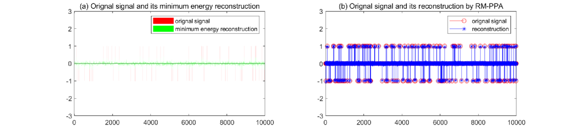
Fig. 1: Comparison results by its minimum energy reconstruction (a) and by RM-PPA with $\theta=0.5$ (b).

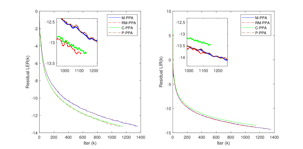
Fig. 2: Convergence behaviors of the residuals LER and LIR by different algorithms.

Next, we consider the problem (21) with large-scale dimensions $(m,n)=(3000,20000)$. By comparing the proposed Algorithms 2.1 (RM-PPA) with the aforementioned tuned parameters to

• Algorithm 2.1 without the relaxation step (“M-PPA”),

• The customized PPA (“C-PPA”, [7]) with parameters $(\gamma,r,s)=(1.8,8,1.02\|A^{\sf T}A\|_{2}/r)$,

• The parameterized PPA (“P-PPA”, [10]) with parameters $(t,r,s)=(-1,8,1.02\|A^{\sf T}A\|_{2}/r)$,

we show comparative results about the convergence behaviors of the residuals $\textrm{LER(k)}:=\log_{2}(\textrm{Eq\_{err}(k)})$ and $\textrm{LIR(k)}:=\log_{2}(\textrm{It\_{err}(k)})$ in Fig. 2, respectively. The effect on recovering the original signal with different algorithms is shown in Fig. 3. Here, we emphasize that the parameter values in [7, 10] can not terminate the algorithms C-PPA and P-PPA because of the fact $\|A^{\sf T}A\|_{2}=1$ for their examples, so we set $r$ the same value as ours but keep $s$ as the value in their experiments. From Figs. 2-3, we observe that M-PPA is competitive to P-PPA and RM-PPA (that is, Algorithm 2.1) performs better than the rest three algorithms.

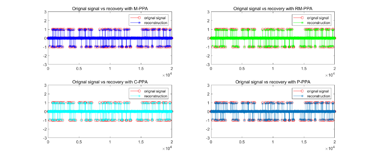
Fig. 3: Comparison results of the problem (21) with $n=20000$ by different algorithms.

References

• [1]
• [2] J. Bai, H. Zhang, J. Li, A parameterized proximal point algorithm for separable convex optimization, Optim. Lett. 12 (2018) 1589-1608.
• [3] J. Bai, J. Liang, K. Guo, Y. Jing, Accelerated symmetric ADMM and its applications in signal processing, (2019) arXiv:1906.12015v2.
• [4] D. Donoho, Y. Tsaig, Fast solution of $l_{1}$-norm minimization problems when the solution may be sparse, IEEE Trans. Inform. Theory, 54 (2008) 4789-4812.
• [5] G. Gu, B. He, X. Yuan, Customized proximal point algorithms for linearly constrained convex minimization and saddle-point problems: a unified approach, Comput. Optim. Appl. 59 (2014) 135-161.
• [6] B. He, F. Ma, X. Yuan, Optimal proximal augmented Lagrangian method and its application to full Jacobian splitting for multi-block separable convex minimization problems, IMA J. Numer. Anal. (2019) doi:10.1093/imanum/dry092.
• [7] B. He, X. Yuan, W. Zhang, A customized proximal point algorithm for convex minimization with linear constraints, Comput. Optim. Appl. 56 (2013) 559-572.
• [8] M. Hestenes, Multiplier and gradient methods, J. Optim. Theory Appl. 4 (1969) 303-320.
• [9] S. Kim, K. Koh, M. Lustig, S. Boyd, D. Gorinvesky, An interior-point method for large-scale $l_{1}$-regularized least squares, IEEE J-STSP, 1 (2007) 606-617.
• [10] F. Ma, M. Ni, A class of customized proximal point algorithms for linearly constrained convex optimization, Comp. Appl. Math. 37 (2018) 896-911.
• [11] B. Martinet, Br$\grave{e}$ve communication, R$\acute{\mbox{e}}$gularisation d’in$\acute{\mbox{e}}$quations variationnelles par approximations successives, ESAIM: Math. Model. Numer. Anal. 4(R3), (1970) 154-159.
• [12] M. Powell, A method for nonlinear constraints in minimization problems, Optimization (R. Fletcher ed.). New York: Academic Press, (1969) 283-298.
• [13] R. Rockafellar, Augmented Lagrangians and applications of the proximal point algorithm in convex programming, Math. Oper. Res. 1(1976) 97-116.
• [14] R. Rockafellar, Monotone operators and the proximal point algorithm, SIAM J. Control Optim. 14, (1976) 97-116.
• [15] J. Yang, X. Yuan, Linearized augmented Lagrangian and alternating direction methods for nuclear norm minimization, Math. Comput. 82 (2013) 301-329.
• [16] Y. Zhu, J. Wu, G. Yu, A fast proximal point algorithm for $l_{1}$-minimization problem in compressed sensing, Appl. Math. Comput. 270 (2015) 777-784.
• [17]