Approximating Free Energy and Committor Landscapes in Standard Transition Path Sampling using Virtual Interface Exchange

Abstract

Transition path sampling (TPS) is a powerful technique for investigating rare transitions, especially when the mechanism is unknown and one does not have access to the reaction coordinate. Straightforward application of TPS does not directly provide the free energy landscape nor the kinetics, which motivated the development of path sampling extensions, such as transition interface sampling (TIS), and the reweighted paths ensemble (RPE), that are able to simultaneously access both kinetics and thermodynamics. However, performing TIS is more involved than TPS, and still requires (some) insight in the reaction to define interfaces. While packages that can efficiently compute path ensembles for TIS are now available, it would be useful to directly compute the free energy from a single TPS simulation. To achieve this, we developed an approximate method, denoted Virtual Interface Exchange, that makes use of the rejected pathways in a form of waste recycling. The method yields an approximate reweighted path ensemble that allows an immediate view of the free energy landscape from a single TPS, as well as enables a full committor analysis.

I Introduction

Molecular simulation of rare event kinetics is challenging, due to the long time scales and high barriers involved Frenkel and Smit (2001); Peters (2017). In the past decades many methods have been invented to overcome this challenge, either via enhanced sampling in configuration space (see e.g. Refs. Torrie and Valleau (1974); Carter et al. (1989); T. Huber, A. Torda, W. van Gunsteren (1994); Grubmüller (1995); Voter (1997); Laio and Parrinello (2002); Darve and Pohorille (2001); Sugita et al. (1999); Marinari and Parisi (1992); Zheng et al. (2008); Gao (2008)), or via path-based methods, that enhance the sampling in trajectory space (see e.g. Refs. Allen et al. (2006); Cerou et al. (2011); Faradjian and Elber (2004); Moroni et al. (2004); Villen-Altamirano and Villen-Altamirano (2002); Berryman and Schilling (2010); Dickson et al. (2009); Huber and Kim (1996); Zhang and Cremer (2010)). Belonging to the latter category, the Transition Path Sampling (TPS) method collects unbiased dynamical trajectories that connect two predefined stable states Dellago et al. (1998); Bolhuis et al. (2002); Dellago et al. (2002); Dellago and Bolhuis (2009). The result is a path ensemble that accurately represents the dynamics of the process of interest, and which can be scrutinised to extract low dimensional descriptions of the reaction coordinate that in turn can be used for determining free energy or kineticsLechner et al. (2010); Bolhuis and Lechner (2011). Notably, projections of the path ensemble on relevant order parameters such as path densities lead to qualitative mechanistic insight. TPS has been successfully applied to complex systems, e.g. protein folding and conformational changesVreede et al. (2010), binding and aggregationSchor et al. (2012); Brotzakis et al. (2017); Brotzakis and Bolhuis (2019), chemical reactions Geissler (2001), and nucleation phenomenaMoroni et al. (2005); Lechner et al. (2011), yielding valuable insight in the reaction coordinate and mechanism.

However, one thing that is not readily available in a standard TPS ensemble is the free energy profile or landscape. This is because the TPS ensemble is a constrained ensemble, which misses information on all the failed paths that did not make it over the barrier, but still contribute significantly to the free energy. This missing information is not easy to correct for in standard TPS. Yet, reliable knowledge of the free energy landscape in the barrier region obtained from TPS simulations would be a very valuable analysis tool. Moreover the standard TPS set up does not provide with the kinetic rate constants directly, and an additional transformation of the path ensemble is neededBolhuis et al. (2002). The TPS methodology suite has been greatly extended over the years. For instance, the transition interface sampling (TIS) version of TPS enable efficient computation of rate constantsvan Erp et al. (2003); Cabriolu et al. (2017). TIS also enables a reweighting of the path ensemble, giving access to the free energy landscapes, and committor surfacesRogal et al. (2010). While there are now software packages that can compute the path ensembles in TIS, this requires a more involved set up, compared to straightforward TPSLervik et al. (2017); Swenson et al. (2019a, b). Indeed, standard transition path sampling has been the entry point for most studies, and it is the first approach one should try, in particular when confronted with a complex transition for which no detailed mechanistic picture is available.

The purpose of this paper is to develop a way to approximate the reweighted path ensemble (RPE) from a single standard TPS run. This approximation is then sufficient to construct the free energy landscape in the barrier region. This approximation is realised by making use of the rejected paths in the TPS sampling, which give information on the free energy barrier. As this approach is making use of the rejected paths, it is a form of waste recycling, a method introduced by Frenkel for reusing rejected Monte Carlo moves Frenkel (2004). In particular, we make use of the virtual replica exchange algorithm by Coluzza and Frenkel Coluzza and Frenkel (2005).

The method is roughly as follows. To compute the RPE we require the TIS ensembles for each interface. However, we only sample the full TPS ensemble. Now, we can interpret each shooting move as a virtual replica exchange move towards the TIS ensemble corresponding to the shooting point, followed by a constrained interface shot. We therefore call this methodology Virtual Interface Exchange TPS (VIE-TPS). Thus, each TPS shot gives an estimate for a particular TIS interface ensemble. From this we can estimate the RPE, and by carefully keeping track of the crossing probabilities we can reweight each (accepted and rejected) trajectory in the ensemble, thus giving the unbiased free energy landscape.

The remainder of the paper is as follows. In the theory section we first briefly recap the TPS and TIS notation. Then we describe the VIE-TPS algorithm. The results section illustrates the new method on a toy model, the AD system, and the FF dimer.

II Theory

II.1 Summary of the TPS, TIS and single replica ensemble

In this section we give a brief overview of the notation for the TPS and TIS ensembles. A trajectory is denoted as $\mathbf{x}\equiv\{x_{1},x_{2}\dots x_{L}\}$, where each frame (or slice, or snapshot) $x$ contains the position and momenta of the entire system at a time $t=i\Delta t$. Frames are thus separated by a time interval $\Delta t$, yielding a trajectory of duration $L\Delta t$. Denoting $\pi[\mathbf{x}]$ as the distribution of paths given by the underlying dynamics (e.g. Langevin dynamics), and introducing two stable state sets A and B, the TPS ensembe is defined as

$$\mathcal{P}_{AB}[\mathbf{x}]=h_{AB}[\mathbf{x}]\pi[\mathbf{x}]/Z_{AB},$$ (1)

here $h_{AB}[\mathbf{x}]$ the indicator function that is only unity if the path connects A with B and $Z_{AB}$ the normalising partition function. In TIS an ordered sequence of interfaces $\lambda_{0},\lambda_{1}\dots\lambda_{n}$ is introduced, parameterised by an order parameter $\lambda$. Denoting the set $\Lambda_{i}=\{x|\lambda(x)>\lambda_{i}\}$, one obtains a similar definition for TIS interface $i$

$$\mathcal{P}_{A\Lambda_{i}}[\mathbf{x}]=\tilde{h}^{A}_{i}[\mathbf{x}]\pi[\mathbf{x}]/Z_{A\Lambda_{i}},$$ (2)

$\tilde{h}^{A}_{i}[\mathbf{x}]$ now the indicator function that is only unity if the path leaves A, crosses $\lambda_{i}$, and then reaches either A or B. The crossing probability connected to the TIS ensemble is:

$$P_{A}(\lambda|\lambda_{i})=\int\mathcal{D}\mathbf{x}\mathcal{P}_{A\Lambda_{i}}[\mathbf{x}]\theta(\lambda_{max}[\mathbf{x}]-\lambda),$$ (3)

where $\mathcal{D}\mathbf{x}$ indicates an integral over all paths, $\theta(x)$ is the Heaviside step function, and $\lambda_{max}[\mathbf{x}]$ returns the maximum value of the $\lambda$ along the path. Here we assumed that $\lambda$ is steadily increasing with $i$.

The shooting move is used to sample both TIS and TPS ensembles:

$$p_{acc}[\mathbf{x}^{(o)}\rightarrow\mathbf{x}^{(n)}]=\tilde{h}_{i}[\mathbf{x}^{(n)}]\min\left[1,\frac{L^{\rm(o)}}{L^{\rm(n)}}\right],$$ (4)

Shooting moves in TIS can be accepted if the path crosses the interface $i$, but need an additional correction factor based on the length. It is also possible to use the constrained interface moveBolhuis (2008), in which the shooting point is chosen among the $n_{\lambda}$ frames that are located at (or near) the interface $\lambda$ (usually defined in some region around the interface). The acceptance criterion for such a constrained move on an interface $j$ is also slight different. In fact, it is determined by the number of frames $n_{\lambda_{j}}$ one is allowed to choose from. The selection probability for a shooting frame is now $p_{sel}(x_{sp})=1/n_{\lambda_{j}}$, instead of $1/L$. The acceptance criterion for a shot from the interface is thus

$$p_{acc}[\mathbf{x}^{(o)}\rightarrow\mathbf{x}^{(n)}]=\tilde{h}_{j}[\mathbf{x}^{(n)}]\min\left[1,\frac{p_{sel}(x^{(n)}_{sp})}{p_{sel}(x^{(o)}_{sp})}\right]$$

$$=\tilde{h}_{j}[\mathbf{x}^{(n)}]\min\left[1,\frac{n_{\lambda_{j}}[\mathbf{x}^{(o)}]}{n_{\lambda_{j}}[\mathbf{x}^{(n)}]}\right]$$ (5)

In single replica TIS (SRTIS) the interface itself is moving location, e.g. from $\lambda_{i}$ to $\lambda_{j}$Du and Bolhuis (2013). This interface move can be accepted with

$$p_{acc}(\mathbf{x};\lambda_{i}\rightarrow\lambda_{j})=\tilde{h}_{j}^{A}[\mathbf{x}]\min\left[1,\frac{g(\lambda_{i})}{g(\lambda_{j})}\right],$$ (6)

where $g(\lambda_{j})$ is the correct density of paths for each interface. This density of paths (DOP) on the interfaces will not be equal for the different interfaces but is high close to stable states, and low close to the transition state region. In fact, the correct DOP is proportional to the crossing probability $g(\lambda_{i})\propto P_{A}(\lambda_{i})$. This can be seen as follows. While an exchange to a lower interface is always possible, an exchange opportunity to a higher interface occurs with the naturally occurring probability for pathways at the higher interfaces, which, in fact, is the crossing probability. To obtain an equal population (for a flat histogram sampling) the exchange acceptance should therefore be biased with the ratio of the crossing probabilities. As an exchange between two interfaces belonging to the same state is governed by the same crossing probability, the proportionality factor cancels.

In the single replica TIS sampling the shooting move and the interface exchange are done separately. It is possible to combine the shooting move and the exchange interface as a single move. This combined shooting and exchange move can be seen as choosing a random interface, and moving the current interface to that position, followed by a shooting move from a shooting point constrained to that interface. When we move to a new interface, the selection of that interface is usually done randomly with a uniform distribution. Hence the selection probability does not appear in the acceptance criterion of Eq.6 . However, we might be using another selection criterion, in particular we would like to use the standard uniform selection of the shooting point on a path to determine the shooting point as well as the interface. When we select a frame from the path uniformly $p_{sel}^{frame}=1/L$, the chance to select a certain interface $i$ is proportional to the number of frames $n_{\lambda_{i}}$ that are close to that interface. In fact it is, $p_{sel}^{(\lambda_{i})}=n_{\lambda_{i}}[\mathbf{x}]/L$. Yet we are using the $p_{sel}^{frame}=1/L$. To correct for this bias, we multiply the (implicit) selection probabilities in the acceptance rule 6, by $p_{sel}^{(\lambda_{i})}$. The acceptance probability is now

$$p_{acc}(\mathbf{x};\lambda_{i}\rightarrow\lambda_{j}])=\tilde{h}_{j}^{A}[\mathbf{x}]\min\left[1,\frac{p_{sel}^{(\lambda_{i})}g(\lambda_{i})}{p_{sel}^{(\lambda_{j})}g(\lambda_{j})}\right]$$

$$=\tilde{h}_{j}^{A}[\mathbf{x}]\min\left[1,\frac{n_{(\lambda_{i})}[\mathbf{x}]g(\lambda_{i})}{n_{(\lambda_{j})}[\mathbf{x}]g(\lambda_{j})}\right],$$ (7)

We can combine the single replica exchange move Eq. II.1 with the constrained shooting move Eq. II.1, yielding

$$P_{\rm acc}(\mathbf{x}^{(o)}\rightarrow\mathbf{x}^{(n)};\lambda_{i}\rightarrow\lambda_{j})=\hfill\tilde{h}_{j}^{A}[\mathbf{x}^{(n)}]\times$$

$$\times\min\left[1,\frac{n_{\lambda_{i}}[\mathbf{x}^{(o)}]g(\lambda_{i})}{n_{\lambda_{j}}[\mathbf{x}^{(n)}]g(\lambda_{j})}\right]$$ (8)

Where again $g(\lambda)\propto P_{A}(\lambda)$.

II.2 Interpreting TPS as SRTIS constrained shooting

Now we can apply this idea also to a straightforward TPS simulation where the interface $i$ is basically fixed at $\lambda_{i}=\lambda_{B}$. The acceptance ratio for a (virtual) single replica shooting move to a new interface $j$ by choosing a uniform frame on the path would then be

$$p_{acc}(\mathbf{x}^{(o)}\rightarrow\mathbf{x}^{(n)};\lambda_{B}\rightarrow\lambda_{j})=\qquad\qquad\qquad\hfill$$

$$=\tilde{h}_{j}^{A}[\mathbf{x}^{(n)}]\min\left[1,\frac{n_{\lambda_{i}}[\mathbf{x}^{(o)}]P_{A}(\lambda_{B})}{n_{\lambda_{j}}[\mathbf{x}^{(n)}]P_{A}(\lambda_{j})}\right]$$

$$=\tilde{h}_{j}^{A}[\mathbf{x}^{(n)}]\min\left[1,\frac{1}{n_{\lambda_{j}}[\mathbf{x}^{(n)}]}\frac{P_{A}(\lambda_{B})}{P_{A}(\lambda_{j})}\right],$$ (9)

Here $n_{\lambda_{B}}[\mathbf{x}^{(o)}]=1$ because the old interface $\lambda_{B}$ only has one point crossing. A major point to make is that the ratio of probabilities ${P_{A}(\lambda_{B})}/{P_{A}(\lambda_{j})}$ in this acceptance ratio is a constant for fixed $\lambda_{j}$. The second remark is that for standard TPS the path can be never accepted, unless it also fulfils

$$p_{acc}[\mathbf{x}^{(o)}\rightarrow\mathbf{x}^{(n)}]={h}_{AB}[\mathbf{x}^{(n)}]\min\left[1,\frac{L^{\rm(o)}}{L^{\rm(n)}}\right],$$ (10)

Paths that do not fulfil this standard TPS condition will be rejected. However we can make use of the rejected paths by waste recyclingFrenkel (2004).

II.3 Making use of Virtual Interface Exhange-TPS

Indeed, virtual Monte Carlo moves have shown to greatly enhance the sampling of the density states Frenkel (2004); Boulougouris and Frenkel (2005). Coluzza and FrenkelColuzza and Frenkel (2005) introduced a virtual replica exchange scheme in which a trial replica exchange move that is rejected can be counted as part of the ensemble. When regular replica exchange is considered, this results in a probability $P_{j}(q)$ for the configuration $q$ in the $j$th replica, based on the exchange probability for replica i and j

$$P_{j}(q)=(1-p_{acc})\delta(q_{j}-q)+p_{acc}\delta(q_{i}-q)$$ (11)

where the first term accounts for non-exchange and recounts the $q_{j}$, the second term for the exchange gives the contribution to $q_{i}$, and where $p_{acc}$ is the acceptance probability for exchange. Extending this to path space gives

$$P_{j}(\mathbf{x})=(1-p_{acc})\delta(\mathbf{x}_{j}-\mathbf{x})+p_{acc}\delta(\mathbf{x}_{i}-\mathbf{x})$$ (12)

Thus if we have two paths $\mathbf{x}_{i}$ and $\mathbf{x}_{j}$ in two path ensembles $i$ and $j$, respectively, then when virtually exchanging these paths between the ensembles, the path ensemble $j$ will have contributions from the ensemble $i$ as specified in this equation. For the single replica exchange shooting move in the TPS ensemble, the first term never contributes, since we are not sampling in the $j$ replica but only in the TPS ensembe $i$. Hence the first delta function does not contribute, leading to

$$P_{j}(\mathbf{x})=p_{acc}=\tilde{h}_{j}^{A}[\mathbf{x}]\min\left[1,\frac{1}{n_{\lambda_{j}}[\mathbf{x}]}\frac{P_{A}(\lambda_{B})}{P_{A}(\lambda_{j})}\right]$$

$$=\frac{1}{n_{\lambda_{j}}[\mathbf{x}]}\frac{P_{A}(\lambda_{B})}{P_{A}(\lambda_{j})},$$ (13)

where the second line follow from the fact that the second argument in the $min$ function is always smaller than unity, if $j<B$, and we only consider paths that start in A. The crossing of the interface $j$ is guaranteed by the constrained interface shooting move. This probability would be less and less likely for trial paths that are shot from an interface $\lambda_{j}$ closer to A. The big point again is that the second factor is constant, not dependent on anything else than $\lambda_{j}$. So, we can take the weight of each path in the $j$th ensemble as ${1}/{n_{\lambda_{j}}[\mathbf{x}{(n)}]}\equiv f[\mathbf{x}]$, times an unknown constant. This weight itself is proportional to the TIS path probability in interface $j$:

$$P_{j}(\mathbf{x})\propto\mathcal{P}_{A\Lambda_{i}}[\mathbf{x}]\propto f[\mathbf{x}]$$ (14)

One can construct standard crossing probability histograms from the ensemble of all trial paths with the same interface $\lambda_{j}$, and hence the same weights according to

$$P_{A}(\lambda|\lambda_{j})=\frac{1}{N_{j}}\sum_{\mathbf{x}}^{N_{j}}\frac{1}{n_{\lambda_{j}}[\mathbf{x}]}\theta(\lambda_{max}[\mathbf{x}]-\lambda),$$ (15)

where $N_{j}$ is the total number of trial paths for $\lambda_{j}$.

The regular, and correct way to construct these crossing probabilities would be to perform TIS on the interface $\lambda_{j}$. Since we aim to get the crossing probability of the virtual interface exchange TPS and TIS identical, the conclusion is that this is only possible if the distribution of shooting points is the same in both cases, and pathways decorrelate quickly. This puts some restriction on the method: in particular it is only correct for two way shooting in the over-damped limit, and when $\lambda$ is reasonably close to the RC.

Nevertheless, even when these conditions are in practice not fulfilled, the crossing probability can be used to approximate the RPE, and hence estimate the free energy surface, as well as the committor surface.

II.4 The VIE-TPS algorithm

The VIE-TPS algorithm is as follows for two-way shooting with uniform selection.

1. Choose a shooting point $sp$ on the current path with uniform selection. Compute $\lambda_{sp}$. Assign the closest interface $j$ e.g. by binning.

2. Alter momenta of the shooting point (e.g. choosing anew from Maxwell Boltzmann distribution, or do random isotropic move) and integrate forward and backward in time until stable states A or B are reached.

3. Identify the path type (AA, AB, BA or BB), and compute the number $n_{\lambda_{sp}}$ of frames located at (in practice near) interface $j$.

4. For paths that start in A do the following:

   1. Assign the trial move to interface $\lambda^{A}_{sp}$ e.g. by binning.

   2. Identify the maximum $\lambda$ on the entire path $\lambda_{max}$ and update the crossing histogram for $\lambda^{A}_{sp}$ by adding $1/n_{\lambda_{sp}}$ to each bin between $\lambda^{A}_{sp}<\lambda<\lambda_{max}$.

5. For paths that start in B do the following:

   1. Assign the trial move to interface $\lambda^{B}_{sp}$ (e.g. by binning).

   2. Identify the minimum lambda on the entire path $\lambda_{min}$ and update the crossing histogram for $\lambda^{B}_{sp}$ by adding $1/n_{\lambda_{sp}}$ to each bin between $\lambda_{min}<\lambda<\lambda_{sp}^{B}$.

6. Store trial path for a posteriori evaluation of the RPE with the assigned path weight $1/n_{\lambda_{sp}}$.

7. Accept trial paths according to the standard TPS criterion Eq.10: if the path does not connect A and B reject the trial path, retaining the previous path. Accept the path according to the length criterion $L^{0}/L^{n}$, reject otherwise.

8. Accumulate transition path ensemble in the normal way.

9. Repeat from step (1) until finished.

Note that while in this algorithm we compute the weights on-the-fly during the TPS sampling, it is also possible to post-process a precomputed TPS ensemble, if all trial paths have been stored.

II.5 Constructing the RPE

After the VIE-TPS sampling the RPE can be constructed from the crossing histograms obtained in steps 4b and 5b, using e.g. WHAMFerrenberg and Swendsen (1989); Kumar et al. (1992), or MBARShirts and Chodera (2008).

First, the total crossing probability histogram is constructed from the individual crossing histograms for all interfaces $i=1\dots n-1$ by applying the WHAM (multiple histogram) method Ferrenberg and Swendsen (1989)

$$P_{A}(\lambda|\lambda_{1})=\sum_{i=1}^{n-1}\bar{w}^{A}_{i}\theta(\lambda_{i+1}-\lambda)\theta(\lambda-\lambda_{i})\sum_{j=1}^{i}P_{A}(\lambda|\lambda_{j})$$ . (16)

The weights $\bar{w}^{A}_{i}$ are given by

$$\bar{w}^{A}_{i}=\frac{1}{\sum_{j=1}^{i}1/w^{A}_{j}},$$ (17)

where $w^{A}_{j}$ are the optimized WHAM weights for each interface histogram $j$.

The RPE is now constructed by reweighting each path (which already had a weight $f[\mathbf{x}]$) with a factor depending on its $\lambda_{max}$ Rogal et al. (2010):

$$\mathcal{P}[\mathbf{x}] = c_{A}\sum_{j=1}^{n-1}\mathcal{P}_{A\Lambda_{j}}[\mathbf{x}]f[\mathbf{x}]W^{A}[\mathbf{x}]$$ (18)

$$+ c_{B}\sum_{j=1}^{n-1}\mathcal{P}_{B\Lambda_{j}}[\mathbf{x}]f[\mathbf{x}]W^{B}[\mathbf{x}],$$

Here $W[\mathbf{x}]=\sum_{i=1}^{n-1}\bar{w}^{A}_{i}\theta(\lambda_{max}[\mathbf{x}]-\lambda_{i})\theta(\lambda_{i+1}-\lambda_{max}[\mathbf{x}])$ selects the correct interface weight for each path $\mathbf{x}$ based on its maximum $\lambda$ value along the trajectory (minumum for BA paths in $W^{B}[\mathbf{x}])$. The unknown constants $c_{A}$ and $c_{B}$ follow from matching the $AB$ and $BA$ histograms for overlapping interfaces  Rogal et al. (2010). This can be most easily done by setting $c_{A}=C/P_{A}(\lambda_{B}|\lambda_{A})$ and $c_{B}=C/P_{B}(\lambda_{A}|\lambda_{B})$, where $C$ is a single (arbitrary) normalising constant

II.6 Projection of the RPE

The free energy then follows from projecting the RPE on a selected set of order parameters ${\mathbf{q}}=\{q_{1},\dots q_{m}\}$ using all trial pathways obtained in step 6 of the algorithm including the rejected ones.

$$F(\boldsymbol{q})=-k_{B}T\ln\rho(\boldsymbol{q})+const,$$ (19)

where we can split up the contributions from the configurational density $\rho(\boldsymbol{q})=\rho_{A}(\boldsymbol{q})+\rho_{B}(\boldsymbol{q})$ into two parts, one related to paths coming from A and one related to path coming from B. For the $N_{A}$ sampled trial paths that start in A (step 4b) $\rho_{A}(\boldsymbol{q})$ becomes

$$\rho_{A}(\boldsymbol{q})=c_{A}\sum_{\mathbf{x}}^{N_{A}}f[\mathbf{x}]W^{A}[\mathbf{x}]\sum_{k=0}^{L}\delta(\boldsymbol{q}(\mathbf{x}_{k})-\boldsymbol{q})$$ (20)

and for the $N_{B}$ sampled trial paths that start in B (step 5b) $\rho_{B}({\boldsymbol{q}})$ becomes

$$\rho_{B}(\boldsymbol{q})=c_{B}\sum_{\mathbf{x}}^{N_{B}}f[\mathbf{x}]W^{B}[\mathbf{x}]\sum_{k=0}^{L}\delta(\boldsymbol{q}(\mathbf{x}_{k})-\boldsymbol{q})$$ (21)

Here $\delta(\boldsymbol{z})=\prod_{i=1}^{m}\delta(z^{(i)})$ is the Dirac delta function, used to project the configurations on to the m-dimensional collective variable space.

When the number of paths is reasonably small, and all paths can be stored on disk then this can be done a posteriori. When the number of paths exceeds storage capacity, one can can save instead of the entire path ensemble, only the histograms for paths ending at $\lambda_{max}$, which requires much less storage. This can be efficiently be done inside the above algorithm by including a simple loop over the current trial path and determine the maximum (or minimum for paths starting in B) and histogram the relevant order parameters in each frame in the path. Then, at the end of the simulation these histograms are reweighted.

Besides the free energy we can project the averaged committor function ${p}_{B}$ on arbitrary surfaces by using the indicator function $h_{B}(x_{L})$.

$$p_{B}({\boldsymbol{q}}) =c_{A}\sum_{\mathbf{x}}^{N_{A}}f[\mathbf{x}]W^{A}[\mathbf{x}]h_{B}(x_{L})$$ (22)

$$+c_{B}\sum_{\mathbf{x}}^{N_{B}}f[\mathbf{x}]W^{B}[\mathbf{x}]h_{B}(x_{L})$$ (23)

Because paths are microscopic reversible, the (averaged) committor function ${p}_{B}({\boldsymbol{q}})$ can aso be defined as the ratio of projected density $\rho_{B}({\boldsymbol{q}})$ of all paths that begin in B to the total density $\rho({\boldsymbol{q}})$ Bolhuis and Lechner (2011):

$${p}_{B}=\frac{\rho_{B}({\boldsymbol{q}})}{\rho_{A}({\boldsymbol{q}})+\rho_{B}({\boldsymbol{q}})}.$$ (24)

The above algoritm is applicable for two-way shooting. For one-way shooting it is also possible to construct the crossing probability, but as the trial paths do not have their backward integration, we cannot assume the full paths to be correct, and hence we cannot construct the FE directly using the above algorithm. However, we might still obtain the free energy by saving for each trial path, for the interface $\lambda_{sp}$, the free energy histogram for values above the interface (below for paths that start in B) and then perform WHAM on these histograms. Note that this does not lead to the RPE, but just to the crossing histograms and free energy as a function fo $\lambda$

Finally as in regular TIS, the rate constant $k_{AB}$ can be calculated as

$$k_{AB}=\frac{\langle\phi_{1,0}\rangle}{\langle h_{A}\rangle}P_{A}(\lambda_{n}|\lambda_{1}),$$ (25)

where the first term is the effective positive flux through the first interface and the second is the crossing probability of interface $n$ of all trajectories shot from interface $i$ and reach state A in their backward integration. The first term is easily accessible through MD and the second through the TIS or as shown in this study through TPS using waste recycling of the rejected paths.

III Simulation methods

We benchmark VIE-TPS in three different examples. We first give a proof of principle with a simple 2D potential. Then we show that the approach works for the standard biomolecular isomerisation of alanine dipeptide. Finally we investigate the dimerisation of solvated FF dipeptides. Below we describe the simulation details for each of these systems.

III.1 Toy model

Consider the 2D potential landscape

$$V[x,y] =0.0177778\left(0.0625x^{4}+y^{4}\right)-e^{-0.3x^{2}-0.01y^{2}}$$

$$-3e^{-0.3(x-4)^{2}-0.01y^{2}}-4e^{-0.3(x+4)^{2}-0.01y^{2}}$$

$$+0.2\sin^{2}(5x)$$ (26)

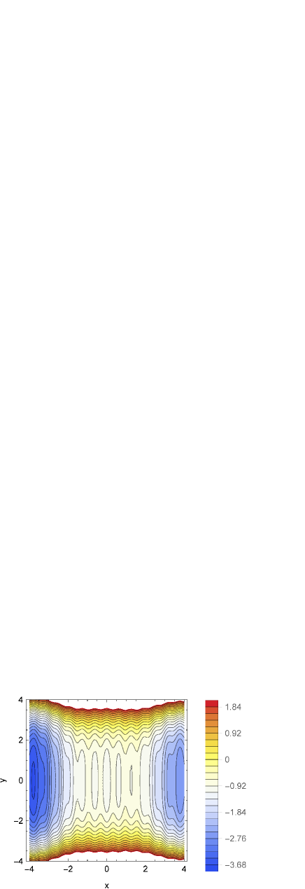
Figure 1: Plot of 2D potential as defined in Eq. 26

The contour plot of this function is shown in Fig. 1. The asymmetric potential consists of two minima with different minimum potential values separated by a high barrier. An oscillatory potential in the x direction is added to make comparisons between different calculations clearer.

We perform TPS simulation at $\beta=3$. For this setting the barrier is about 10 kT. We use three different dynamics: Metropolis Monte Carlo dynamicsFrenkel and Smit (2001), Langevin dynamics at high friction $\gamma=10$ and a medium friction $\gamma=2.5$. For the MC we use a maximum step size of

We perform TPS on this potential with an initial stable state A defined by $x<-3.5$ and a final stable state B defined by $x>3.5$. During the TPS the crossing probability and the RPE were constructed using the algorithm above. The RPE was used to construct the FE.

III.2 Alanine Dipeptide

We perform atomistic molecular dynamics simulations of Alanine Dipeptide (AD) using the Gromacs 4.5.4 engine Pronk et al. (2013), employing the AMBER96 Bayly et al. (1995) and TIP3P force fields Jorgensen et al. (1983). The system is prepared as follows: First, the AD molecule is placed in a cubic box of 28 x 28 x 28 $\rm\AA$ followed by an energy minimisation. The system is thereafter solvated, energy minimized, shortly equilibrated for 1 ns, and finally subjected to a production run of 75 $ns$ NPT simulation. NPT simulations are carried out at ambient conditions. Bonds are constrained using the Lincs algorithm, Van Der Waals interactions are cut off at 1.1 nm, and electrostatics are treated using the Particle Mesh Ewald method using a Fourier spacing of 0.12 nm and a cut-off of 1.1 nm for the short range electrostatics. The leap-frog algorithm is used to propagate the dynamics, and the neighbour list is updated every 10 fs, using a 1.1 nm cut-off and a 2 fs time step. The temperature and pressure are kept constant using the v-rescale thermostat Bussi et al. (2007) and Parrinello-Rahman Parrinello, M. and Rahman (1981) barostat, respectively.

We use TPS to sample transition paths connecting the $\alpha$ to $\beta$ state. The $\alpha$ state spans the volume of $-150^{\circ}\leq\psi\leq-60^{\circ}$ and $-180^{\circ}\leq\phi\leq 0^{\circ}$, and in turn the $\beta$ state spans the volume of $150^{\circ}\leq\psi\leq 180^{\circ}$ and $-180^{\circ}\leq\phi\leq 0^{\circ}$. Note that such state definitions are rather strict. The initial path is obtained from the 75 ns MD run. The two-way shooting, with randomized velocities and flexible-length TPS variant is used. Frames are saved every 0.03 ps and the maximum allowed transition path length is 30 ps. The crossing probabilities were calculated along the $\psi$ order parameter.

III.3 FF dimer

The details of the atomistic molecular dynamics simulation of the FF dimer are identical to the ones in Brotzakis and Bolhuis (2016). We briefly outline it below. We perform atomistic molecular dynamics simulations of the FF dimer using the Gromacs 4.5.4 engine Pronk et al. (2013), employing the AMBER99SB-ILDN Lindorff-Larsen et al. (2010) and TIP3P force fields Jorgensen et al. (1983). The FF segment is isolated from the KLVFFA sequence (residues 16-21) of the amyloid-beta peptide (PDB2Y29 Colletier (2011)) and subsequently capped with neutral ACE and NME termini. The system is prepared as follows: First, two FF monomers are placed in a cubic box of 30 x 30 x 30 $\rm\AA$ followed by an energy minimization. The system is thereafter solvated, energy minimized, shortly equilibrated for 10 ns, and finally subjected to a production run of 200 ns NPT simulation. NPT simulations are carried out at ambient conditions. Bonds are constrained using the Lincs algorithm, Van Der Waals interactions are cut off at 1 nm, and electrostatics are treated using the Particle Mesh Ewald method using a Fourier spacing of 0.12 nm and a cut-off of 1 nm for the short range electrostatics. The leap-frog algorithm is used to propagate the dynamics, and the neighbour list is updated every 10 fs, using a 1 nm cut-off and a 2 fs time step. The temperature and pressure are kept constant using the v-rescale thermostat Bussi et al. (2007) and Parrinello-Rahman Parrinello, M. and Rahman (1981) barostat, respectively.

We use TPS to sample transition paths connecting the bound to unbound state. The bound state ($B$) spans the volume of minimum distance $\leq$ 0.22 nm, and in turn the unbound state ($U$) the volume of minimum distance $\geq$ 1.1 nm. The initial path is obtained from the 200 ns MD run. The two-way shooting, with randomized velocities and flexible-length TPS variant is used. Frames are saved every 5 ps and the maximum allowed transition path length is 10 ns. The crossing probabilities were calculated along the minimum distance order parameter.

IV Results and Discussion

IV.1 Toy model

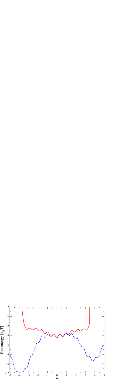
Figure 2: Free energy along the x-axis estimated by a) direct integration of the potential (blue) and b) the negative logarithm of the configurations generated from TPS (red).

For an easier comparison we compute the free energy always as a 1-D projection along the x-axis. The exact projection of Eq. 26 is given in Fig. 2 as a blue dashed line. The red curve is the negative logarithm of probability to observe configuration is the path ensemble obtained from direct projection of the paths on the x-axis. This curve shows that clearly a naive projection of the TPS ensemble will not remotely be close to the true free energy.

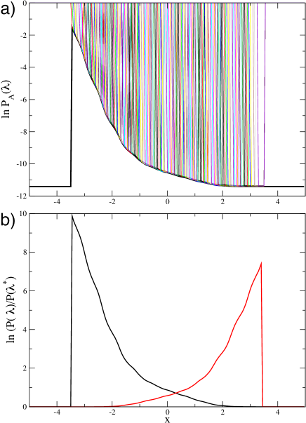
Figure 3: a) Crossing probability for AB paths. Solid black line is WHAM result. All other curves come from histograms for $\lambda_{sp}$. b) Crossing probability from WHAM for forward and reverse histograms, normalised to their final value $P(\lambda^{*})$

In Fig. 3a we plot for the Metropolis Monte Carlo dynamics TPS the individual crossing probabilities for the forward transition AB reweighted according to WHAM. The final histogram is also shown as a solid black curve. The lower panel shows the reweighted crossing probabilities for the forward and backward transition, both using the correct relative weight. From this it is directly possible to construct the RPE, which can be used to compute the free energy profiles.

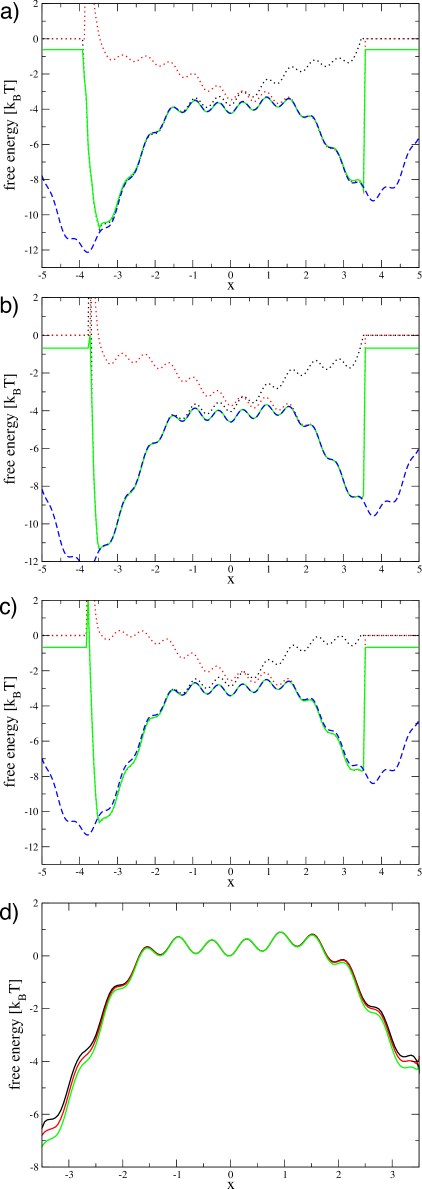
Figure 4: Forward (black dotted), backward (red dotted), overall TPS (green) and reference (blue dashed) free energies for a) Monte Carlo, b) Langevin high friction, and c) Langevin low friction dynamics panels respectively. In the panel c) we show the free energy profiles of the Monte Carlo, Langevin high friction, and Langevin low friction dynamics together.

In Fig. 4 we show the free energy profile for each of three different dynamics case. Also shown is the individual forward and backward contribution to the free energy. Note that both for Metropolis dynamics and medium high friction the agreement with the true free energy is excellent. For the low friction case the comparison is slightly less favorable, but still very reasonable. The discrepancy is most likely caused by some memory in the dynamics. The comparison between all three dynamics is shown in panel Fig. 4c. Again, while there is some discrepancy at the barrier flanks, the agreement in the barrier region is excellent.

VIE-TPS assumes that the distribution of shooting points along the interfaces is identical or at least close to the correct distribution in the corresponding TIS ensemble. For diffusive dynamics this assumption is reasonable, because paths decorrelate fast, and sample the (local) equilibrium distribution. For ballistic dynamics decorrelation is slower and the shooting point distribution from the reactive path ensemble is not necessary identical to that of the TIS ensemble. In addition, the presence of other channels and dead ends along the interaces that are not sampled in the reactive AB path ensemble will be present in the TIS ensemble, and contribute to the correct FE projection. This will result in an overestimation of the freen energy in the minima, something that we indeed observe.

Finally we show that the obtained RPE can reconstruct the free energy in arbitrary dimensions. Since we have only a 2D potential, this is by necessity a reconstruction of the original 2D potential from the 1D based RPE. To make this more interesting we slightly adjusted the potential to

$$V[x,y] =0.0177778\left(0.0625x^{4}+y^{4}\right)-3e^{-0.3(x-4)^{2}-0.01y^{2}}$$

$$-3e^{-0.3(x+4)^{2}-0.01y^{2}}+e^{-3(x+1)^{2}-0.1(y-2)^{2}}$$

$$+e^{-3(x-1)^{2}-0.1(y+2)^{2}}$$ (27)

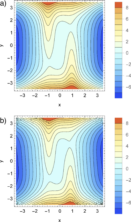
Figure 5: Free energy surface of the potential of Eq. 27 constructed by a) analytical integration b) the virtual Interface exchange TPS scheme.

This potential, shown in Fig. 5a, has again a two minima, but now the barrier region is convoluted in the y-direction. The 1D projection clearly does not contain this information. Yet, by projection of the RPE from a single TPS simulation the entire landscape is reconstructed. Note that this reconstruction is only possible due to the RPE, as by standard histogramming of the free energy, this information is lost.

Having access to the RPE and using Eq. 23 we project the committor along the xy dimensions for the potential of Eq. 26. Remarkably, the committor isolines twist at the barrier, as suggested by the underlying potential and hint towards a non linear reaction coordinate. Indeed, it is possible to use these surfaces to conduct a reaction coordinate analysis Lechner et al. (2010)

IV.2 Alanine Dipeptide

Alanine dipeptide in water exhibits a conformational transition between states $\alpha$ and $\beta$ in the timescale of hundreds of $ps$ Du and Bolhuis (2013). Yet, the equilibration in the basins is in the order of few $ps$, thus making the transition a rare event. The short transition time compared to today’s computational capacities has made alanine dipeptide a toy biomolecular model for benchmarking enhanced sampling methods to brute force MD. We first benchmark VIE-TPS with a long brute force MD by projecting the free energy as a function of the $\psi$ angle (see Fig. 7a). The agreement is good in the barrier region and within 0.5 $kT$ in the region $-50^{\circ}\leq\phi\leq 80^{\circ}$. We attribute the discrepancy in the free energy closer to state $\beta$ to the memory trajectories have when 1) The dynamics is not diffusive enough, 2) the length of the transition paths is short. For alanine dipeptide the average path length is small ($\approx$ 5 $ps$). This is the reason that this method should be used with strict state definitions. This discrepancy will be reduced for larger and more realistic transition times (as also shown in the next example). VIE-TPS can be used to reweight and project the Free Energy Surface (FES) as a function of any order parameter. By projecting the RPE along $\phi$ and $\psi$, we compare VIE-TPS and MD estimates of the FES (see Fig. 7b,c). As in the 1D projection, the FES is best estimated in the barrier region. Strikingly, VIE-TPS is able to resolve well two transition state regions, a higher one $-80^{\circ}\leq\psi\leq-60^{\circ}$ , $0^{\circ}\leq\phi\leq 30^{\circ}$ and a lower one $-150^{\circ}\leq\psi\leq-125^{\circ}$ , $0^{\circ}\leq\phi\leq 30^{\circ}$ as was also found in Ref. Bolhuis et al. (2000). Moreover, the statistics and representation of the barrier region is much finer in the VIE-TPS than in MD, which has an exponentially rarer sampling of that region. Finally using VIE-TPS and Eq. 23, one can reconstruct the committor surface along any arbitrary order parameter. We plot the committor surface along $\Psi$ (see Fig. 7d) and find that the isocommittor surface of 0.5 is located at the barrier region, discussed earlier. We note that the committor surface estimated in this way is much less error prone than calculating the committor directly through the shooting points.

VIE-TPS can be used to directly calculate transition rates from a single TPS and a short MD in states A and B simulation using Eq. 15 and  Eq. 25. For the forward rate $k_{\alpha\beta}$, by selecting $\lambda_{0}$ at $\psi$=-60^∘ and $\lambda_{1}$ at $\psi$=-50^∘ and $\lambda_{n}$ at $\psi$=150^∘ the estimated flux factor is 1.34 ps^-1 and the crossing probability term is 0.039 (see Fig. 8), thus giving a rate of 0.052 ps^-1, which is less than a factor of two different from the respective rate of 0.0298 ps^-1 coming from brute force MD. On the other hand, for the backward rate $k_{\beta\alpha}$ by selecting $\lambda_{0}$ at $\psi$=150^∘ and $\lambda_{1}$ at $\psi$=140^∘ and $\lambda_{n}$ at $\psi$=-60^∘ the estimated flux factor is 0.66 ps^-1 and the crossing probability term is 0.01 (see Fig. 8), thus giving a rate of 0.009 ps^-1, which is only a factor of two different from the respective rate of 0.004 ps^-1 coming from brute force MD. These results are in fairly good agreement with Refs Swenson et al. (2019a); Du and Bolhuis (2013). With this rates at hand, the free energy difference between stable states $\alpha$ and $\beta$, estimated as $\Delta G_{\alpha\beta}$=-log($\frac{k_{\beta\alpha}}{k_{\alpha\beta}}$), is 2.04 $kT$ and 1.72 $kT$ from MD and VIE-TPS respectively. This way of estimating the free energy difference between stable states gives more accurate results compared to the ones from the RPE free energy estimate (see Fig. 7). However, we stress once more that the VIE-TPS method gives only approximate results.

IV.3 FF dipeptide dimerization

In the final illustrative example we focus on the dimerization of two phenylalanine dipeptides as in Ref. Brotzakis and Bolhuis (2016), shown in Fig. 9. The hydrophobicity of these peptides causes their dimerization, while entropy stabilizes the monomer state. The relaxation time in the basins is in the order of several $ns$, however the transition time is in the order of $ps$, classifying dimerization a rare transition. We benchmark VIE-TPS by comparing the MD estimate of the FES as a function of $d_{min}$, and find excellent agreement between the two (see Fig. 10a). VIE-TPS is able to capture the details of the FES at the first and second hydration shell minima (0.5 $nm$ and 0.8 $nm$). As in alanine dipeptide, there is a 0.5 $kT$ difference close to the unbound stable state (distances greater than 0.9 $nm$). Note that the FES estimate from the brute force MD increases again after the minimum at 0.8 $nm$ due to the finite size of the system. In reality, the FES as a function of the minimum distance at the unbound state should have been a plateau (as estimated by VIE-TPS).

By using the RPE information we can reweight the FES to a different order parameter, such as the solvent accessible surface (see Fig. 10b). The agreement between the two ways of calculating the FES is excellent. We attribute the better agreement of this system compared to the alanine dipeptide to the longer transition paths ($\approx$ 400 ps) and the clearly diffusive dynamics of this system.

V Conclusion

In this paper we have presented a way to extract (an approximation of) the reweighted path ensemble from a single standard (two state) TPS simulation employing the uniform two-way shooting algorithm. This has the great advantage that an estimate for the kinetics, the free energy, and the committor landscape can be directly given. We showed that the method approximates the RPE well in the barrier region, but is less accurate at the flanks towards the stables state, especially for dynamics with a large ballistic component. Nevertheless, we believe this will be very useful for deterministic dynamics, in which stochasticity plays a role, as is the case in most complex biomolecular transition.

We note that the RPE can be used for a reaction coordinate analysis, e.g. using the likelihood methods of Peters and TroutPeters and Trout (2006), or more advanced machine learning techniques. Finally, the free energies and committor surfaces can be used in conjunction with the Bayesian TPT formulas of Hummer Hummer (2004) in order to alternatively calculate rate coefficients. We expect that this methodology will be soon part of the standard tools in packages such as OPS. Our method can be easily extended to multiple state TPS.

VI Acknowledgement

The authors thank Georgios Boulougouris and Bernd Ensing for carefully commenting the manuscript. We acknowledge support from the Nederlandse Organisatie voor Wetenschappelijk Onderzoek (NWO) for the use of supercomputer facilities. Z.F.B. would like to acknowledge the Federation of European Biochemical Societies (FEBS) for financial support (LTF).

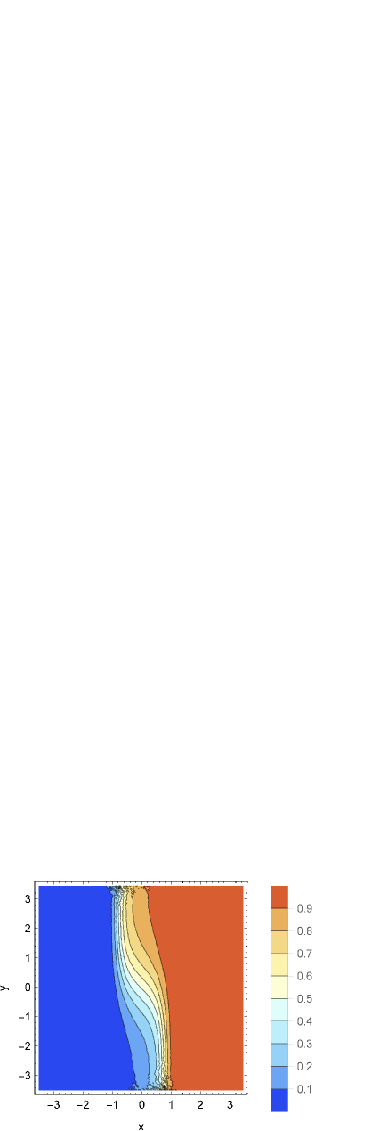
Figure 6: Committor surface for potential in Eq. 27

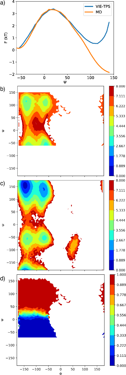
Figure 7: Free energy surface of $\alpha$ to $\beta$ transition of AD as a function of a) the $\Psi$ angle, where in blue and orange are depicted the VIE-TPS and MD predictions respectively and $\Phi$ and $\Psi$ coming from b) VIE-TPS RPE and c) MD. d) Committor surface projected on $\Phi$ and $\Psi$.

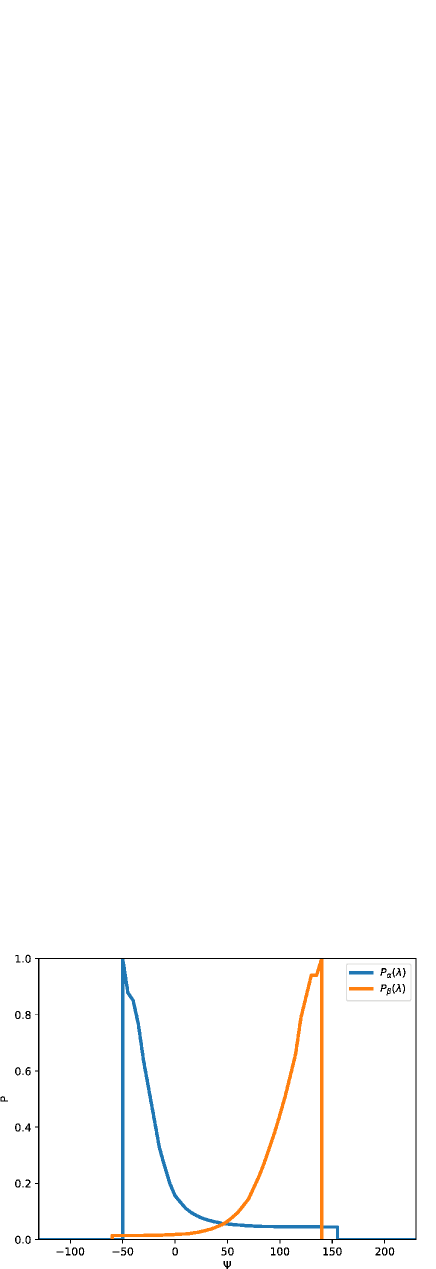
Figure 8: Crossing probability from WHAM, as a function of the order parameter $\Psi$ for path coming from states $\alpha$ (in blue) and $\beta$ (in green) respectively.

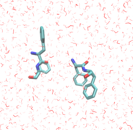
Figure 9: Snapshot of a configuration of the FF dipeptide dimer in solution, coming from an association/dissociation transition path.

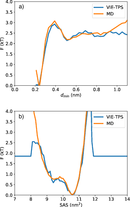
Figure 10: Free energy surface as a function of a) the minimum distance (d_min) between the two peptides and b) the solvent accessible surface (SAS). In blue and orange are depicted the VIE-TPS and MD predictions respectively.

References

- Frenkel and Smit (2001) D. Frenkel and B. Smit, Understanding Molecular Simulation, 2nd ed. (Academic Press, Inc., Orlando, FL, USA, 2001).
- Peters (2017) B. Peters, Reaction Rate Theory and Rare Events (Elsevier Science, Amsterdam, 2017).
- Torrie and Valleau (1974) G. M. Torrie and J. P. Valleau, Chem. Phys. Lett. 28, 578 (1974).
- Carter et al. (1989) E. Carter, G. Ciccotti, J. T. Hynes, and R. Kapral, Chem. Phys. Lett. 156, 472 (1989).
- T. Huber, A. Torda, W. van Gunsteren (1994) T. Huber, A. Torda, W. van Gunsteren, J. Comput. Aided Mol. Des. 8, 695 (1994).
- Grubmüller (1995) H. Grubmüller, Phys. Rev. E 52, 2893 (1995).
- Voter (1997) A. F. Voter, J. Chem. Phys. 106, 4665 (1997).
- Laio and Parrinello (2002) A. Laio and M. Parrinello, Proc. Nat. Acad. Sci. USA 99, 12562 (2002).
- Darve and Pohorille (2001) E. Darve and A. Pohorille, J. Chem. Phys. 115, 9169 (2001).
- Sugita et al. (1999) Y. Sugita, , and Y. Okamoto, Chem. Phys. Lett. 314, 141 (1999).
- Marinari and Parisi (1992) E. Marinari and G. Parisi, Europhys. Lett. 19, 451 (1992).
- Zheng et al. (2008) L. Zheng, M. Chen, and W. Yang, Proc. Natl. Acad. Sci. U.S.A. 105, 20227 (2008).
- Gao (2008) Y. Q. Gao, J. Chem. Phys. 128, 064105 (2008).
- Allen et al. (2006) R. Allen, D. Frenkel, and P. ten Wolde, J. Chem. Phys. 124, 024102 (2006).
- Cerou et al. (2011) F. Cerou, A. Guyader, T. Lelievre, and D. Pommier, J. Chem. Phys. 134, xx (2011).
- Faradjian and Elber (2004) A. K. Faradjian and R. Elber, J. Chem. Phys. 120, 10880 (2004).
- Moroni et al. (2004) D. Moroni, P. G. Bolhuis, and T. S. van Erp, J. Chem. Phys. 120, 4055 (2004), https://doi.org/10.1063/1.1644537 .
- Villen-Altamirano and Villen-Altamirano (2002) M. Villen-Altamirano and J. Villen-Altamirano, Eur. Trans. Telecom. 13, 373 (2002).
- Berryman and Schilling (2010) J. T. Berryman and T. Schilling, J. Chem. Phys. 133, 244101 (2010).
- Dickson et al. (2009) A. Dickson, A. Warmflash, and A. R. Dinner, J. Chem. Phys. 131, 154104 (2009).
- Huber and Kim (1996) G. Huber and S. Kim, Biophys. J. 70, 97 (1996).
- Zhang and Cremer (2010) Y. Zhang and P. S. Cremer, Annu. Rev. Phys. Chem. 61, 63 (2010).
- Dellago et al. (1998) C. Dellago, P. G. Bolhuis, F. S. Csajka, and D. Chandler, J. Chem. Phys. 108, 1964 (1998).
- Bolhuis et al. (2002) P. G. Bolhuis, D. Chandler, C. Dellago, and P. L. Geissler, Annu. Rev. Phys. Chem. 53, 291 (2002).
- Dellago et al. (2002) C. Dellago, P. G. Bolhuis, and P. L. Geissler, Adv. Chem. Phys. 123, 1 (2002).
- Dellago and Bolhuis (2009) C. Dellago and P. G. Bolhuis, Adv Polym Sci 221, 167 (2009).
- Lechner et al. (2010) W. Lechner, J. Rogal, J. Juraszek, B. Ensing, and P. G. Bolhuis, J. Chem. Phys. 133, 174110 (2010).
- Bolhuis and Lechner (2011) P. G. Bolhuis and W. Lechner, J. Stat. Phys. 145, 841 (2011).
- Vreede et al. (2010) J. Vreede, J. Juraszek, and P. G. Bolhuis, Proc. Natl. Acad. Sci. U. S. A. 107, 2397 (2010).
- Schor et al. (2012) M. Schor, J. Vreede, and P. G. Bolhuis, Biophysical Journal 103, 1296 (2012).
- Brotzakis et al. (2017) Z. F. Brotzakis, M. Gehre, I. K. Voets, and P. G. Bolhuis, Phys. Chem. Chem. Phys. 19, 19032 (2017).
- Brotzakis and Bolhuis (2019) Z. F. Brotzakis and P. G. Bolhuis, J. Phys. Chem. B (2019), 10.1021/acs.jpcb.8b10005.
- Geissler (2001) P. L. Geissler, Science 291, 2121 (2001).
- Moroni et al. (2005) D. Moroni, P. R. Ten Wolde, and P. G. Bolhuis, Phys. Rev. Lett. 94, 1 (2005).
- Lechner et al. (2011) W. Lechner, C. Dellago, and P. G. Bolhuis, Physical Review Letters 106 (2011), 10.1103/physrevlett.106.085701.
- van Erp et al. (2003) T. S. van Erp, D. Moroni, and P. G. Bolhuis, J. Chem. Phys. 118, 7762 (2003).
- Cabriolu et al. (2017) R. Cabriolu, K. M. S. Refsnes, P. G. Bolhuis, and T. S. van Erp, J. Chem. Phys. 147, 152722 (2017).
- Rogal et al. (2010) J. Rogal, W. Lechner, J. Juraszek, B. Ensing, and P. G. Bolhuis, J. Chem. Phys. 133, 174109 (2010).
- Lervik et al. (2017) A. Lervik, E. Riccardi, and T. S. van Erp, J. Comput. Chem. 38, 2439 (2017).
- Swenson et al. (2019a) D. W. Swenson, J. H. Prinz, F. Noe, J. D. Chodera, and P. G. Bolhuis, J. Chem. Theory Comput. 15, 813 (2019a).
- Swenson et al. (2019b) D. W. Swenson, J. H. Prinz, F. Noe, J. D. Chodera, and P. G. Bolhuis, J. Chem. Theory Comput. 15, 837 (2019b).
- Frenkel (2004) D. Frenkel, Proceedings of the National Academy of Sciences 101, 17571 (2004).
- Coluzza and Frenkel (2005) I. Coluzza and D. Frenkel, ChemPhysChem 6, 1779 (2005).
- Bolhuis (2008) P. G. Bolhuis, J. Chem. Phys. 129 (2008), 10.1063/1.2976011.
- Du and Bolhuis (2013) W. Du and P. G. Bolhuis, J. Chem. Phys. 139, 044105 (2013).
- Boulougouris and Frenkel (2005) G. C. Boulougouris and D. Frenkel, J. Chem. Theory Comput. 1, 389 (2005).
- Ferrenberg and Swendsen (1989) A. M. Ferrenberg and R. H. Swendsen, Physical Review Letters 63, 1195 (1989).
- Kumar et al. (1992) S. Kumar, J. M. Rosenberg, D. Bouzida, R. H. Swendsen, and P. A. Kollman, Journal of Computational Chemistry 13, 1011 (1992).
- Shirts and Chodera (2008) M. R. Shirts and J. D. Chodera, The Journal of Chemical Physics 129, 124105 (2008).
- Pronk et al. (2013) S. Pronk, S. Páll, R. Schulz, P. Larsson, P. Bjelkmar, R. Apostolov, M. R. Shirts, J. C. Smith, P. M. Kasson, D. van der Spoel, B. Hess, and E. Lindahl, Bioinformatics 29, 845 (2013).
- Bayly et al. (1995) C. I. Bayly, K. M. Merz, D. M. Ferguson, W. D. Cornell, T. Fox, J. W. Caldwell, P. A. Kollman, P. Cieplak, I. R. Gould, and D. C. Spellmeyer, J. Am. Chem. Soc. 117, 5179 (1995).
- Jorgensen et al. (1983) W. L. Jorgensen, J. Chandrasekhar, J. D. Madura, R. W. Impey, and M. L. Klein, J. Chem. Phys. 79, 926 (1983).
- Bussi et al. (2007) G. Bussi, D. Donadio, and M. Parrinello, J. Chem. Phys. 126, 014101 (2007).
- Parrinello, M. and Rahman (1981) A. Parrinello, M. and Rahman, J Appl. Phys. 52, 7182 (1981).
- Brotzakis and Bolhuis (2016) Z. F. Brotzakis and P. G. Bolhuis, J. Chem. Phys. 145, 164112 (2016).
- Lindorff-Larsen et al. (2010) K. Lindorff-Larsen, S. Piana, K. Palmo, P. Maragakis, J. L. Klepeis, R. O. Dror, and D. E. Shaw, Proteins 78, 1950 (2010).
- Colletier (2011) J. Colletier, PNAS 108, 16938 (2011).
- Bolhuis et al. (2000) P. G. Bolhuis, C. Dellago, and D. Chandler, Proc. Natl. Acad. Sci. U.S.A. 97, 5877 (2000).
- Peters and Trout (2006) B. Peters and B. L. Trout, J. Chem. Phys. 125, 054108 (2006).
- Hummer (2004) G. Hummer, J. Chem. Phys. 120, 516 (2004).