Asymptotic reductions of the diffuse-interface model,
with applications to contact lines in fluids

Abstract

The diffuse-interface model (DIM) is a tool for studying interfacial dynamics. In particular, it is used for modeling contact lines, i.e., curves where a liquid, gas, and solid are in simultaneous contact. As well as all other models of contact lines, the DIM implies an additional assumption: that the flow near the liquid/gas interface is isothermal. In this work, this assumption is checked for the four fluids for which all common models of contact lines fail. It is shown that, for two of these fluids (including water), the assumption of isothermality does not hold.

I Introduction

The single most important open problem in hydrodynamics is that of contact lines, i.e., curves where a liquid, gas, and solid are in simultaneous contact (such as, for example, the circumference of a droplet on a substrate). It has been known for almost fifty years HuhScriven71 that the Navier–Stokes equations and the standard boundary conditions fail near a moving contact line, yet there seems to be no consensus as to how this issue can be resolved BonnEggersIndekeuMeunierRolley09; Velarde11. The problem is caused by the no-slip condition preventing the fluid particles on the contact line from moving – hence, the contact line itself is pinned to the substrate. As a result, numerous phenomena involving wetting/dewetting (e.g., sliding droplets) can be neither understood nor modeled.

Several attempts to remedy the problem have been made – typically, by modifying the boundary condition at the substrate in such a way that, near a contact line, the fluid can slip (e.g., Refs. HuhMason77; BenneyTimson80; Hocking1981; Gouin87; Shikhmurzaev93; Sharma93; Shikhmurzaev97; BenilovVynnycky13). In some cases, different models agree with each other, in others they do not SibleySavvaKalliadasis12; SibleyNoldSavvaKalliadasis14. Furthermore, it has been recently shown PuthenveettilSenthilkumarHopfinger13; BenilovBenilov15 that there are several fluids including water, for which none of the commonly used models produces physically meaningful results.

Most importantly, all existing models of contact lines have one feature in common: they assume that the flow near a liquid/vapor interface is isothermal. In addition, most theories assume that the Reynolds number based on the interfacial thickness is small. Yet, neither of these assumptions has been verified. Direct measurements at such small scales are extremely difficult to carry out, and nor can one draw conclusions about an interface from the characteristics of the global flow: even if the latter is isothermal, the interface may not be.

Indeed, the high-gradient nature of the near-interface region can give rise to strong production of heat due to viscosity and compressibility, as well as evaporation and condensation. The released heat may cause strong, albeit local, temperature variations, which can significantly affect the dynamics of the contact line – as can fluid inertia if the local Reynolds number is large.

In the present work, the so-called diffuse-interface model is used to check the assumptions of isothermality and small Reynolds number for four fluids for which the common models of contact lines fail. It is demonstrated that, for water and mercury examined in Refs. PodgorskiFlessellesLimat01; WinkelsPetersEvangelistaRiepenEtal11, at least one of the assumptions does not hold. For glycerol and ethylene glycol examined in Ref. KimLeeKang02, both assumptions actually hold – hence, the discrepancies between the experiments and theory in this case are due to different reasons (to be discussed later).

This paper has the following structure. In Sect. II, the diffuse-interface model (DIM) is formulated. In Sect. III, the DIM is reduced to several simpler sets of equations, depending on the parameters of the fluid under consideration. In Sect. IV, the properties of the asymptotic sets are examined, and Sect. V outlines how the present results can be made more comprehensive and accurate.

II Formulation

Consider a flow of a non-ideal fluid characterized by its density $\rho(\mathbf{r},t)$, velocity $\mathbf{v}(\mathbf{r},t)$, pressure $p(\mathbf{r},t)$, and temperature $T(\mathbf{r},t)$, where $\mathbf{r}$ is the position vector and $t$, the time. Let the equation of state be of the van der Waals type, i.e.,

$$p=\frac{RT\rho}{1-b\rho}-a\rho^{2},$$ (1)

where $R$ is the specific gas constant, and $a$ and $b$ are the van der Waals parameters.

There exist several versions of the DIM, which have been applied to numerous physically-important problems HohenbergHalperin77; JasnowVinals96; LowengrubTruskinovsky98; VladimirovaMalagoliMauri99; PismenPomeau00; ThieleMadrugaFrastia07; DingSpelt07; MadrugaThiele09; YueZhouFeng10; YueFeng11; SibleyNoldSavvaKalliadasis13a; SibleyNoldSavvaKalliadasis13b; MagalettiMarinoCasciola15; MagalettiGalloMarinoCasciola16; KusumaatmajaHemingwayFielding16; FakhariBolster17; GalloMagalettiCasciola18; BorciaBorciaBestehornVarlamovaHoefnerReif19; GalloMagalettiCoccoCasciola20; GelissenVandergeldBaltussenKuerten20; Benilov20a. More comprehensive versions (e.g., Refs. AndersonMcFaddenWheeler98; ThieleMadrugaFrastia07) are applicable to multi-component fluids with variable temperature, simpler ones apply either to single-component isothermal fluids (e.g., Ref. PismenPomeau00) or single-component isothermal and incompressible fluids (e.g., Refs. JasnowVinals96; DingSpelt07; MadrugaThiele09).

In the present paper, the non-isothermal compressible DIM for a single-component fluid will be used, in the form suggested in Ref. AndersonMcFaddenWheeler98.

The governing equations of the version of the DIM suggested in Ref. AndersonMcFaddenWheeler98 are

$$\frac{\partial\rho}{\partial t}+\boldsymbol{\boldsymbol{\nabla}}\cdot\left(\rho\mathbf{v}\right)=0,$$ (2)

$$\frac{\partial\mathbf{v}}{\partial t}+\left(\mathbf{v}\cdot\boldsymbol{\boldsymbol{\nabla}}\right)\mathbf{v}+\frac{1}{\rho}\boldsymbol{\boldsymbol{\nabla}}\cdot\left(\mathbf{I}p-\boldsymbol{\Pi}\right)=K\boldsymbol{\boldsymbol{\nabla}}\nabla^{2}\rho,$$ (3)

$$\rho c_{V}\left(\frac{\partial T}{\partial t}+\mathbf{v}\cdot\boldsymbol{\boldsymbol{\nabla}}T\right)+\left(p+a\rho^{2}\right)\boldsymbol{\boldsymbol{\nabla}}\cdot\mathbf{v}\\ -\boldsymbol{\Pi}:\boldsymbol{\boldsymbol{\nabla}}\mathbf{v}=\boldsymbol{\boldsymbol{\nabla}}\cdot\left(\kappa\boldsymbol{\boldsymbol{\nabla}}T\right),$$ (4)

where $\mathbf{I}$ is the identity matrix, the viscous stress tensor is

$$\boldsymbol{\Pi}=\mu_{s}\left[\boldsymbol{\boldsymbol{\nabla}}\mathbf{v}+\left(\boldsymbol{\boldsymbol{\nabla}}\mathbf{v}\right)^{T}-\frac{2}{3}\mathbf{I}\left(\boldsymbol{\boldsymbol{\nabla}}\cdot\mathbf{v}\right)\right]+\mu_{b}\mathbf{I}\left(\boldsymbol{\boldsymbol{\nabla}}\cdot\mathbf{v}\right),$$ (5)

$\mu_{s}$ ($\mu_{b}$) is the shear (bulk) viscosity, $c_{V}$ is the specific heat capacity, and $\kappa$ is the thermal conductivity, and the right-hand side of (3) represents the so-called Korteweg stress ($K$ is a fluid-specific constant). Note that $\mu_{s}$, $\mu_{b}$, $c_{V}$, and $\kappa$ are fluid-specific functions of $\rho$ and $T$.

Let the fluid be enclosed in a container (mathematically speaking, domain) $\mathcal{D}$, so that

$$\mathbf{v}=\mathbf{0}\qquad\text{at}\qquad\mathbf{r}\in\partial\mathcal{D},$$ (6)

where $\partial\mathcal{D}$ is the container’s walls (domain’s boundary). Another boundary condition should be imposed on $T$; assuming for simplicity that the walls are insulated, let

$$\mathbf{n}\cdot\boldsymbol{\boldsymbol{\nabla}}T=0\qquad\text{at}\qquad\mathbf{r}\in\partial\mathcal{D},$$ (7)

where $\mathbf{n}$ is a normal to $\partial\mathcal{D}$.

Several versions of the boundary condition for $\rho$ exist in the literature Seppecher96; PismenPomeau00; SoucekHeidaMalek20. In this work, the simplest one is used,

$$\mathbf{n}\cdot\boldsymbol{\boldsymbol{\nabla}}\rho=0\qquad\text{at}\qquad\mathbf{r}\in\partial\mathcal{D},$$ (8)

which is a particular case of the condition derived in Ref. Seppecher96.

Generally, little in the analysis to come depends on the specific form of the boundary conditions (7)-(8). They are mostly needed for numerical simulations reported in Sect. IV.

III Simplified models

III.1 Nondimensionalization

Assuming that the pressure gradient across the interface is balanced by the Korteweg stress, one can deduce that the spatial scale of interfacial dynamics is

$$\bar{r}=\left(\frac{K}{a}\right)^{1/2}.$$

Introduce also a velocity scale $\bar{v}$ (so that the time scale is $\bar{r}/\bar{v}$), a characteristic temperature $\bar{T}$, and the density scale $b^{-1}$.

The following nondimensional variables will be used:

$$\mathbf{r}_{nd}=\frac{\mathbf{r}}{\bar{r}},\qquad t_{nd}=\frac{\bar{v}}{\bar{r}}t,$$

$$\rho_{nd}=b\rho,\qquad\mathbf{v}_{nd}=\frac{\mathbf{v}}{\bar{v}},\qquad T_{nd}=\frac{T}{\bar{T}}.$$

It is convenient to also introduce the nondimensional versions of the fluid parameters. Assume for simplicity that the bulk and shear viscosities are of the same order (say, $\bar{\mu}$), and denote the other two scales by $\bar{\kappa}$ and $\bar{c}_{V}$, so that

$$\left(\mu_{s}\right)_{nd}=\frac{\mu_{s}}{\bar{\mu}},\qquad\left(\mu_{b}\right)_{nd}=\frac{\mu_{b}}{\bar{\mu}},$$

$$\kappa_{nd}=\frac{\kappa}{\bar{\kappa}},\qquad\left(c_{V}\right)_{nd}=\frac{c_{V}}{\bar{c}_{V}},$$

and the nondimensional viscous stress is

$$\boldsymbol{\Pi}_{nd}=\frac{\bar{r}}{\bar{\mu}\bar{v}}\boldsymbol{\Pi}.$$

In the most general situation, the viscous stress, the Korteweg stress, and the pressure gradient in Eq. (3) are all of the same order, which implies

$$\bar{v}=\frac{a\bar{r}}{\bar{\mu}b^{2}}.$$

Physically, this scale characterizes the disbalance between the Korteweg stress and pressure gradient (typically arising if the interface is curved); most importantly, it has nothing to do with the global flow.

Rewriting Eqs. (1)-(4) in terms of the nondimensional variables and omitting the subscript _nd, one obtains

$$\frac{\partial\rho}{\partial t}+\boldsymbol{\boldsymbol{\nabla}}\cdot\left(\rho\mathbf{v}\right)=0,$$ (9)

$$\framebox{$\alpha$}\left[\frac{\partial\mathbf{v}}{\partial t}+\left(\mathbf{v}\cdot\boldsymbol{\boldsymbol{\nabla}}\right)\mathbf{v}\right]\\ +\frac{1}{\rho}\boldsymbol{\boldsymbol{\nabla}}\cdot\left[\mathbf{I}\left(\frac{\framebox{$\tau$}T\rho}{1-\rho}-\rho^{2}\right)-\boldsymbol{\Pi}\right]=\boldsymbol{\boldsymbol{\nabla}}\nabla^{2}\rho,$$ (10)

$$\framebox{$\alpha\gamma$}\rho c_{V}\left(\frac{\partial T}{\partial t}+\mathbf{v}\cdot\boldsymbol{\boldsymbol{\nabla}}T\right)\\ +\framebox{$\beta$}\left(\frac{\framebox{$\tau$}T\rho}{1-\rho}\boldsymbol{\boldsymbol{\nabla}}\cdot\mathbf{v}-\boldsymbol{\Pi}:\boldsymbol{\boldsymbol{\nabla}}\mathbf{v}\right)=\boldsymbol{\boldsymbol{\nabla}}\cdot\left(\kappa\boldsymbol{\boldsymbol{\nabla}}T\right),$$ (11)

where

$$\alpha=\frac{K}{\bar{\mu}^{2}b^{3}},\qquad\beta=\frac{aK}{\bar{\mu}\bar{\kappa}\bar{T}b^{4}},$$ (12)

$$\gamma=\frac{\bar{c}_{V}\bar{\mu}}{\bar{\kappa}},\qquad\tau=\frac{R\bar{T}b}{a}.$$ (13)

Judging by the positions of $\alpha$ and $\beta$ in Eqs. (11)-(12), $\alpha$ is the Reynolds number and $\beta$, an ‘isothermality parameter’. The latter controls the production of heat due to compressibility and viscosity, i.e., if $\beta\ll 1$, the flow is close to isothermal. In turn, $\gamma$ is the Prandtl number and $\tau$ is the nondimensional temperature.

It should be emphasized that $\alpha$ and $\beta$ are ‘microscopic’ parameters. They characterize the flow at the interfacial scale and they do not depend on either the global Reynolds number (based on, say, the droplet’s size) nor on whether or not the flow is isothermal globally.

The nondimensional expression for $\boldsymbol{\Pi}$ and the nondimensional boundary conditions will not be presented, as they look exactly as their dimensional counterparts (5)-(8).

III.2 Asymptotic estimates

A lot of valuable information can be extracted by estimating the nondimensional parameters (12)-(13) for the four liquids for which discrepancies between experimental and theoretical results have been reported. To do so, one needs the parameters of these fluids – all of which, except $K$, have been found in Ref. HaynesLideBruno17 and collated, for the reader’s convenience, in Appendix A). $K$, in turn, was calculated by relating it to the surface tension (see Appendix B). The temperature scale was set to $\bar{T}=25^{\circ}\mathrm{C}$, which is regarded in Ref. HaynesLideBruno17 as the “normal temperature” and is also close to the “room temperature” at which experiments are normally conducted.

At this temperature, the viscosity, specific heat, and thermal conductivity of the liquid phase of all fluids considered exceed those of the vapor phase by several orders of magnitude. Thus, the variations of these parameters across the interface are approximately equal to the liquid values – which were thus used to estimate the nondimensional parameters involved.

The estimated values of $\alpha$, $\beta$, $\alpha\gamma$, and $\tau$ are presented in Table 1. The following conclusions can be drawn:

Fluid	$\alpha$	$\beta$	$\alpha\gamma$	$\tau$
ethylene glycol	$5\times 10^{-4}$	$0.033$	$0.073$	$0.123$
glycerol	$2\times 10^{-7}$	$6\times 10^{-4}$	$2\times 10^{-3}$	$0.104$
mercury	$2.63$	$0.390$	$0.066$	$0.050$
water	$0.143$	$0.711$	$0.880$	$0.137$

Table 1: The nondimensional parameters (12)-(13) for fluids under consideration.

1. The assumption of small Reynolds number, $\alpha\ll 1$, does not hold for mercury.

2. The isothermality assumption, $\beta\ll 1$, does not hold for mercury, and even less so, for water.

3. On a less important note, $\tau$ seems to be moderately small for all four fluids. This impression is misleading, however, as the values of $\tau$ in Table 1 are comparable to the maximum of this parameter, $\tau=8/27$ (corresponding to the critical temperature of the van der Waals fluid).

Thus, it comes as no surprise that all of the existing theories of contact lines fail for mercury and water – but their failure for glycerol and ethylene glycol must be caused by different reasons. For example, the discrepancy associated with the latter pair of fluids might be due to chemical inhomogeneity of the substrate, as inhomogeneities are known to dramatically affect the dynamics of contact lines SavvaKalliadasis13.

In principle, there could be additional reasons for the failure of the existing models for the four fluids at issue – but, in case of mercury and water, these reasons must be sought using non-isothermal models.

III.3 Asymptotic equations

Depending on the fluid under consideration, the exact governing equations can be reduced to a simpler asymptotic set. Three of these will be presented: for mercury (Set 1), water (Set 2), and glycerol and ethylene glycol (Set 3).

To obtain Set 1, assume

$$\alpha\sim 1,\qquad\beta\sim 1,\qquad\alpha\gamma\ll 1,$$

and omit the terms involving $\alpha\gamma$ from the governing equations. The density and momentum equations (9)-(10) remain the same, whereas Eq. (11) becomes

$$\beta\left(\frac{\tau T\rho}{1-\rho}\boldsymbol{\boldsymbol{\nabla}}\cdot\mathbf{v}-\boldsymbol{\Pi}:\boldsymbol{\boldsymbol{\nabla}}\mathbf{v}\right)-\boldsymbol{\boldsymbol{\nabla}}\cdot\left(\kappa\boldsymbol{\boldsymbol{\nabla}}T\right)=0.$$ (14)

With the time derivative omitted from this equation, $T$ is ‘enslaved’ by (instantly adjusts to) the heat production due to compressibility and viscosity.

Given an initial condition for $\rho$ and $\mathbf{v}$, Eqs. (9)-(10), (14), expression (5) for $\boldsymbol{\Pi}$, and the boundary conditions (6)-(8) fully determine $\rho(\mathbf{r},t)$, $\mathbf{v}(\mathbf{r},t)$, $T(\mathbf{r},t)$.

To obtain Set 2, let

$$\alpha\ll 1,\qquad\beta\sim 1,\qquad\alpha\gamma\sim 1,$$ (15)

and omit the terms involving $\alpha$. The density equation (9) and that for the temperature (11) remain the same, whereas Eq. (10) becomes

$$\frac{1}{\rho}\boldsymbol{\boldsymbol{\nabla}}\cdot\left[\mathbf{I}\left(\frac{T\rho}{1-\rho}-\rho^{2}\right)-\boldsymbol{\Pi}\right]=\boldsymbol{\boldsymbol{\nabla}}\nabla^{2}\rho.$$ (16)

Eqs. (9), (16), (11), and (5), and the boundary conditions (6)-(8) form a full set. This time, the velocity does not require an initial condition, as it is ‘enslaved’ by $\rho$ and $T$ through Eq. (16) and boundary condition (6).

To obtain Set 3, assume

$$\alpha\ll 1,\qquad\beta\ll 1,\qquad\alpha\gamma\ll 1.$$

The density equation (9) remains as is, the velocity equation is the same as (16), whereas (11) becomes

$$\boldsymbol{\boldsymbol{\nabla}}\cdot\left(\kappa\boldsymbol{\boldsymbol{\nabla}}T\right)=0.$$

This equation and the boundary condition (7) imply that

$$T=T(t).$$ (17)

To determine $T(t)$, one needs to return to the exact equation (11), integrate it over the domain $\mathcal{D}$ and take into account the boundary condition (7) – so that the leading-order term disappears, resulting

$$c_{V}M\frac{\mathrm{d}T}{\mathrm{d}t}+T\int_{\mathcal{D}}\frac{\rho}{1-\rho}\boldsymbol{\boldsymbol{\nabla}}\cdot\mathbf{v}\,\mathrm{d}^{3}\mathbf{r}-\int_{\mathcal{D}}\boldsymbol{\Pi}:\boldsymbol{\boldsymbol{\nabla}}\mathbf{v}\,\mathrm{d}^{3}\mathbf{r}=0,$$ (18)

where

$$M=\int_{\mathcal{D}}\rho\,\mathrm{d}^{3}\mathbf{r}$$

is constant due to the mass conservation law.

Eqs. (9), (16), (18), and (5), and the boundary conditions (6), (8) form a full set. The initial condition for $T$ should not depend on the spatial variables, as initial variations of $T$ (if any) are implied to rapidly even out, so that the flow almost instantly becomes isothermal.

In most applications, the container is so large that $M\gg 1$. In this case, Eq. (18) yields $\mathrm{d}T/\mathrm{d}t\approx 0$ – hence, in the other equations, $T$ can be treated as a known constant determined by the initial condition. The resulting model is mathematically equivalent to the one examined in Ref. PismenPomeau00.

IV Properties of the asymptotic models

Given that it is nearly impossible to separate phase transition from hydrodynamic motion, it is vital that the derived asymptotic models satisfy the fundamental requirements of thermodynamics: firstly, they should comply with the Maxwell construction and, secondly, predict the correct threshold of the instability responsible for phase transitions. In what follows, both requirements will be illustrated for the simplest of the sets derived, Set 3.

Consider the one-dimensional reduction of Set 3, i.e., let $v_{1}=v_{2}=0$, with the rest of the unknowns depending only on $r_{3}$ and $t$. Denoting $v_{3}=w$ and $r_{3}=z$, and considering for simplicity the large-container limit, one can reduce Eqs. (9), (16), and 5), and the boundary conditions (6) and (8) to

$$\frac{\partial\rho}{\partial t}+\frac{\partial\left(\rho w\right)}{\partial z}=0,$$ (19)

$$\frac{1}{\rho}\frac{\partial}{\partial z}\left(\frac{T\rho}{1-\rho}-\rho^{2}-\eta\frac{\partial w}{\partial z}\right)=\frac{\partial^{3}\rho}{\partial z^{3}},$$ (20)

$$w=0,\qquad\frac{\partial\rho}{\partial z}=0\qquad\text{at}\qquad z=\pm\frac{1}{2}Z,$$ (21)

where $\eta=\frac{4}{3}\mu_{s}+\mu_{b}$ and $Z$ is the container size.

It can be readily shown that:

• Steady solutions – such that $w=0$, $\rho=\rho(z)$ – of Eqs. (19)-(21) with $Z=\infty$ describe a stationary liquid/vapor interface in an infinite domain. It can be readily shown that, for these solutions,

  $$\lim\limits_{{}_{z\rightarrow-\infty}}\left(\frac{T\rho}{1-\rho}-\rho^{2}\right)=\lim\limits_{z\rightarrow-\infty}\left(\frac{T\rho}{1-\rho}-\rho^{2}\right),$$

  $$\lim\limits_{z\rightarrow-\infty}\left[T\left(\ln\frac{\rho}{1-\rho}+\frac{1}{1-\rho}\right)-2\rho\right]\\ =\lim\limits_{z\rightarrow\infty}\left[T\left(\ln\frac{\rho}{1-\rho}+\frac{1}{1-\rho}\right)-2\rho\right],$$

  which is the van der Waals version of the Maxwell construction, according to which the pressures and the densities of Gibbs free energy of the two phases must be equal.

• As shown in Appendix C, a single-phase state characterized by a pair $\left(T,\rho\right)$ and governed by Eqs. (19)-(21) in an infinite domain is unstable, if

  $$\frac{T}{\left(1-\rho\right)^{2}}-2\rho<0,$$ (22)

  which is the van der Waals version of the thermodynamic instability criterion FerzigerKaper72

  $$\left(\dfrac{\partial p}{\partial\rho}\right)_{T}<0.$$

  Given that this instability triggers off phase transitions, one should hope that the asymptotic equations describe those well.

The boundary-value problem (19)-(21) was simulated numerically using the method of lines Schiesser78, for various initial conditions and various examples of the viscosity $\eta(\rho,T)$. As expected, two patterns of dynamics were observed: the solution would evolve either toward a single-phase state or a two-phase state.

An example of the latter behavior was computed for the following (nondimensional) viscosity:

$$\eta=\frac{\rho}{1-\rho},$$ (23)

for the nondimensional temperature

$$T=0.25,$$ (24)

and the initial condition

$$\rho=0.3+0.005\sin\frac{\pi z}{Z}.$$ (25)

Criterion (22) predicts that steady state (24)-(25) is unstable – which it indeed is, as can be seen in Fig. 1. Evidently, the solution evolves into the two-phase state described by the Maxwell construction.

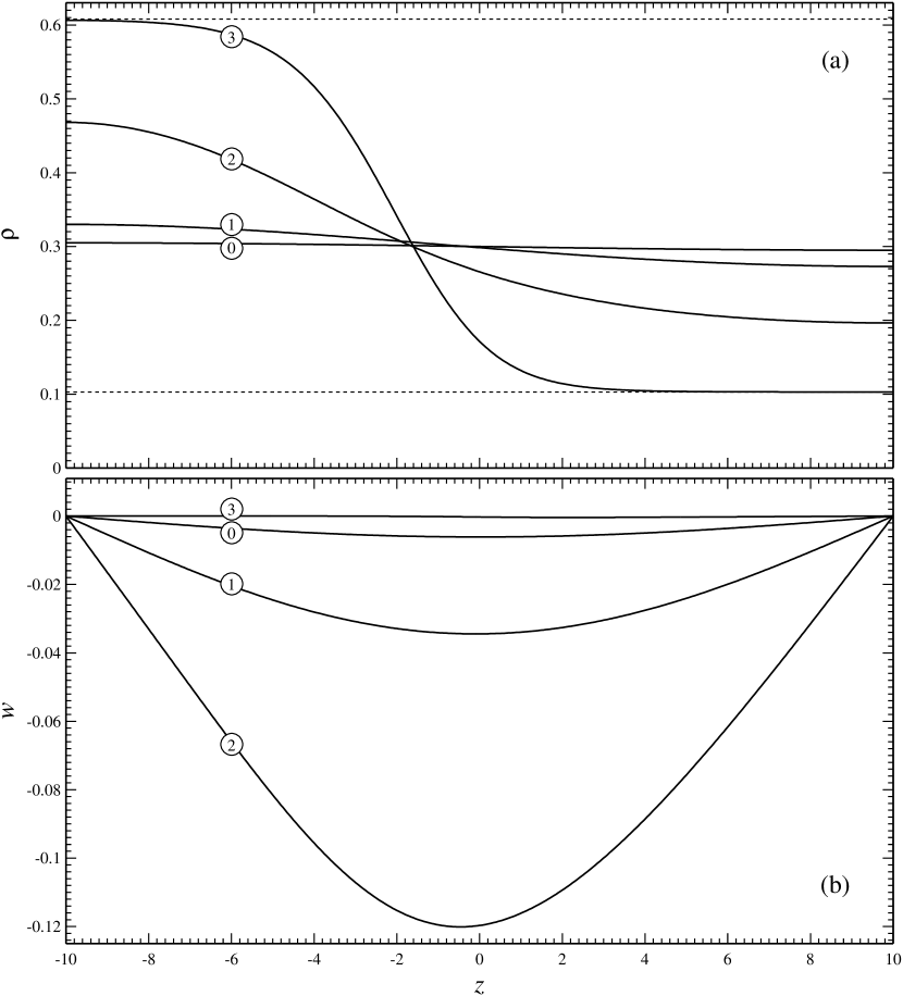
Figure 1: The solution of Eqs. (19)-(21) and (23), with $Z=20$ and the initial condition (24). The curves labeled “0”, “1”, “2”, “3” correspond to $t=0,~{}30,~{}60,~{}300$, respectively. (a) The density field (the dotted lines show the liquid and vapor densities predicted by the Maxwell construction). (b) The velocity field.

V Concluding remarks

Thus, depending on the fluid under consideration, the diffuse-interface model can be reduced to one of three possible sets of asymptotic equations. Only one of the three satisfies the assumptions on which the existing models of contact lines are based, so no new results should be expected in this case. The other two asymptotic sets should go beyond the existing models, describing fluids to which these models do not apply (such as water and mercury).

In addition to the four fluids included in the present paper another four have been examined (acetone, benzene, ethanol, and methanol). Only for one of these $\alpha$ is small, and none have isothermal interfaces – which makes one wonder whether the failure of these assumptions is an exception or rule. They seems to hold only for high-viscosity fluids, such as glycerol and ethylene glycol, as well as (probably) silicone oils which are frequently used in experiments with contact lines. This hypothesis, however, remains unverified, as the full set of characteristics of any of silicone oils does not seem to be available, neither in the literature nor internet.

As this work is only a proof of concept, there are a number of extensions of the DIM to be considered in the future – such as introduction of pair correlations MaitrejeanAmmarChinestaGrmela12, non-Newtonian viscosity, non-Fourier heat conduction, and self-diffusion Grmela14; VanPavelkaGrmela17. Such extensions should be relatively easy do develop using the so-called GENERIC tool GrmelaOttinger97; OettingerGrmela97, and they should make the asymptotic models proposed in this paper more comprehensive and accurate. It is also crucial to give up the van der Waals equation of state and use a realistic one, describing the fluid under consideration with a sufficient accuracy (this has already been done for water Benilov20a).

Appendix A The parameters of the fluids under consideration

All of the parameters listed in this appendix have been taken from Ref. HaynesLideBruno17.

The van der Waals constants $a$ and $b$ were calculated using the critical temperature $T_{c}$ and the critical pressure $p_{c}$, through the formulae (see Ref. HaynesLideBruno17)

$$a=\frac{27R^{2}T_{c}^{2}}{64p_{c}m^{2}},\qquad b=\dfrac{RT_{c}}{8p_{c}m},$$ (26)

where $m$ is the molar mass. The results, as well as the ‘source data’, are presented in Table 2.

Fluid	$m~{}(\mathrm{g~{}mol}^{-1})$	$T_{c}~{}(\mathrm{K})$	$p_{c}~{}(\mathrm{MPa})$	$a~{}(\mathrm{m}^{5}\mathrm{s}^{-2}\mathrm{kg}^{-1})$	$b~{}(\mathrm{m}^{3}\mathrm{g}^{-1})$
ethylene glycol	$62.07$	$719$	$8.1$	$483.13$	$1.4863$
glycerol	$92.09$	$850$	$7.6$	$326.93$	$1.2622$
mercury	$200.59$	$1764$	$167$	$13.506$	$0.0547$
water	$18.02$	$647.10$	$22.06$	$1704.8$	$1.6918$

Table 2: The molar masses, the critical temperatures and pressures, and the van der Waals parameters [determined by (26)] of the fluids under consideration.

Fluid	$\bar{\mu}~{}(\mathrm{mPa~{}s})$	$\bar{\kappa}~{}(\mathrm{W~{}m}^{-1}\mathrm{K}^{-1})$	$\bar{c}_{p}~{}(\mathrm{kJ~{}kg}^{-1}\mathrm{K}^{-1})$	$\sigma~{}(\mathrm{mN~{}m}^{-1})$
ethylene glycol	$16.06$	$0.254$	$2.394$	$48.02$
glycerol	$934$	$0.285$	$2.377$	$62.5$
mercury	$1.526$	$8.514$	$0.114$	$485.48$
water	$0.890$	$0.6062$	$4.179$	$72.06$

Table 3: The dynamic viscosities, thermal conductivities, specific heat capacities, and surface tensions of the fluids under consideration (all at $25^{\circ}\mathrm{C}$).

Table 3, in turn, presents the dynamic viscosities, thermal conductivities, specific heat capacities, and surface tensions. Note that Ref. HaynesLideBruno17 does not present data on $\bar{c}_{V}$ which was used for nondimensionalizing the governing equations, so $\bar{c}_{p}$ was used instead, so that the assumption $\bar{c}_{V}\approx\bar{c}_{p}$ was implied. Admittedly, it does not hold for gases, but does do for liquids (for water, for example, $\bar{c}_{V}\approx 4.13~{}\mathrm{kJ~{}kg}^{-1}\mathrm{K}^{-1}$ and $\bar{c}_{p}\approx 4.18~{}\mathrm{kJ~{}kg}^{-1}\mathrm{K}^{-1}$). Besides, $\bar{c}_{p}$ is used in this paper as a scale for $\bar{c}_{V}$, so its precise value is unimportant.

Appendix B Deducing $K$ from a liquid’s surface tension

Within the framework of the DIM, the surface tension of a liquid/vapor interface can be related to the solution of the static one-dimensional reduction of Eqs. (1)-(5). Setting, accordingly, $\partial/\partial t=0$, $\mathbf{v}=\mathbf{0}$, and $\rho=\rho(z)$, one obtains

$$\frac{1}{\rho}\left[\frac{RT}{\left(1-b\rho\right)^{2}}-2a\rho\right]\frac{\mathrm{d}\rho}{\mathrm{d}z}=K\frac{\mathrm{d}^{3}\rho}{\mathrm{d}z^{3}}.$$ (27)

This equation is to be solved in an unbounded domain under the condition

$$\frac{\mathrm{d}\rho}{\mathrm{d}z}\rightarrow 0\qquad\text{as}\qquad z\rightarrow\pm\infty.$$ (28)

Once the boundary-value problem (27)-(28) is solved and its solution $\rho(z)$ is found, the surface tension of liquid/vapor interface is given by Mauri13

$$\sigma=K\int_{-\infty}^{\infty}\left(\frac{\mathrm{d}\rho}{\mathrm{d}z}\right)^{2}\mathrm{d}z.$$ (29)

Now, assume that the real-life value of $\sigma$ has been measured at a certain temperature $\bar{T}$. To determine $K$ in this case, one should solve the boundary-value problem (27)-(28) for $T=\bar{T}$ while varying $K$ – until the result computed through (29) coincides with the measured $\sigma$. Note that, even though this approach depends on the choice of $\bar{T}$, the resulting $K$ is supposed to apply to the whole temperature range between the triple and critical points (as the DIM assumes that $K$ does not depend on $T$).

Computed with $\bar{T}=25^{\circ}\mathrm{C}$, the values of $K$ for the fluids under consideration are presented in Table 4.

Fluid	$K\times 10^{16}~{}(\mathrm{m}^{7}\mathrm{kg}^{-1}\mathrm{s}^{-2})$
ethylene glycol	$16.06$
glycerol	$934$
mercury	$1.526$
water	$0.890$

Table 4: The Korteweg parameter of the fluids under consideration, computed using the approach described in Appendix B

Note that expression (29) represents the surface tension of a liquid/vapor interface – whereas the data  in Ref. HaynesLideBruno17 are for the liquid/air one. However, these parameters are close: for water at $25^{\circ}\mathrm{C}$, for example, the former is $\sigma=71.97~{}\mathrm{mN~{}m}^{-1}$ WagnerKretzschmar08 and the latter is $\sigma=72.06$ $\mathrm{mN~{}m}^{-1}$ HaynesLideBruno17.

Appendix C Derivation of the instability criterion (22)

Consider a homogeneous state characterized by a density $\bar{\rho}$ and temperature $\bar{T}$; assume also that the fluid is at rest, $\bar{w}=0$, and let the solution have the form

$$\rho=\bar{\rho}+\tilde{\rho}(t,z),\qquad w=\tilde{w}(t,z),$$

where the tilded variable represent a small perturbation. Substituting the above expressions into Eqs. (19)-(20), then linearizing them and omitting overbars, one obtains

$$\frac{\partial\tilde{\rho}}{\partial t}+\rho\frac{\partial\tilde{w}}{\partial z}=0,$$ (30)

$$\frac{1}{\rho}\frac{\partial}{\partial z}\left[\frac{T\tilde{\rho}}{\left(1-\rho\right)^{2}}-2\rho\tilde{\rho}-\eta\frac{\partial\tilde{w}}{\partial z}\right]=\frac{\partial^{3}\tilde{\rho}}{\partial z^{3}},$$ (31)

Only harmonic disturbances will be examined, i.e.

$$\tilde{\rho}=\hat{\rho}\operatorname{e}^{ikz+\lambda t},\qquad\tilde{w}=\hat{w}\operatorname{e}^{ikz+\lambda t},$$ (32)

where $k$ is the perturbation’s wavenumber and $\lambda$, its growth/decay rate. If, for some $k$, $\operatorname{Re}\lambda>0$, the state characterized by $\left(\rho,T\right)$ is unstable.

Substituting (32) into (30)-(31), one obtains

$$\lambda\hat{\rho}+i\rho k\hat{w}=0,\qquad\frac{1}{\rho}\left[\frac{T\hat{\rho}}{\left(1-\rho\right)^{2}}-2\rho\hat{\rho}-ik\eta\hat{w}\right]=-k^{2}\hat{\rho}.$$

These equations admit a solution for $\hat{\rho}$ and $\hat{w}$ only if

$$\lambda=-\frac{\rho}{\eta}\left[\frac{T}{\left(1-\rho\right)^{2}}-2\rho+k^{2}\rho\right],$$

which shows that a value of $k$ exists such that $\lambda>0$ only subject to condition (22).