A new scheme for fixed node diffusion quantum Monte Carlo with pseudopotentials: improving reproducibility and reducing the trial-wave-function bias

Abstract

Fixed node diffusion quantum Monte Carlo (FN-DMC) is an increasingly used computational approach for investigating the electronic structure of molecules, solids, and surfaces with controllable accuracy. It stands out among equally accurate electronic structure approaches for its favorable cubic scaling with system size, which often makes FN-DMC the only computationally affordable high-quality method in large condensed phase systems with more than 100 atoms. In such systems FN-DMC deploys pseudopotentials to substantially improve efficiency. In order to deal with non-local terms of pseudopotentials, the FN-DMC algorithm must use an additional approximation, leading to the so-called localization error. However, the two available approximations, the locality approximation (LA) and the T-move approximation (TM), have certain disadvantages and can make DMC calculations difficult to reproduce. Here we introduce a third approach, called the determinant localization approximation (DLA). DLA eliminates reproducibility issues and systematically provides good quality results and stable simulations that are slightly more efficient than LA and TM. When calculating energy differences – such as interaction and ionization energies – DLA is also more accurate than the LA and TM approaches. We believe that DLA paves the way to the automization of FN-DMC and its much easier application in large systems.

I Introduction

A wide range of scientific topics greatly benefit from computer simulations, such as crystal polymorph prediction, molecular adsorption on surfaces, the assessment of phase diagrams, phase transitions, nucleation, and more. The accuracy of the computational methods employed for such simulations is of fundamental importance. In a wide range of physical-chemical problems many important static, dynamic, and thermodynamic properties are related to the potential energy surface. Thus, one of the grand challenges of computational modelling is the evaluation of accurate energetics for molecules, surfaces and solids. This challenge is far from straightforward, because various types and strengths of interatomic and intermolecular interactions are relevant, and a method must describe all of them correctly.

There are various computational methods acknowledged for having high accuracy. For condensed phase systems one very promising methodology is quantum Monte Carlo (QMC),Foulkes et al. (2001) often in the fixed-node (FN) diffusion Monte Carlo (DMC) flavor. FN-DMC has favorable scaling with system size (between the 3-rd and the 4-th power of the system size) and it can be efficiently deployed on high performance computer facilities. Nowadays there is an increasing amount of benchmark data for solids and surfaces obtained via FN-DMC.Zen et al. (2018); Brandenburg et al. (2019); Zen et al. (2016a); Al-Hamdani et al. (2017a, b, 2015); Trail et al. (2017); Luo et al. (2017); Dubecký et al. (2016); Devaux et al. (2015); Wu et al. (2015); Zheng and Wagner (2015); Wagner and Abbamonte (2014); Azadi et al. (2014); Benali et al. (2016); Shin et al. (2017); Ahn et al. (2018); Tsatsoulis et al. (2017); Doblhoff-Dier et al. (2017) Data provided by DMC is of use in tackling interesting materials science problems and also to help the improvement of density functional theory (DFT)Maurer et al. (2019) and other cheaper computational approaches.

DMC implements a technique to project out the exact ground state wave function $\Phi$ from a trial wave function $\Psi_{T}$ by performing a propagation according to the imaginary time-dependent Schrödinger equation.Foulkes et al. (2001) However, an unconstrained projection leads to a bosonic wave function, so in fermionic systems the fixed-node (FN) approximation is typically employed to keep the projected wave function antisymmetric. FN-DMC constrains the projected wave-function $\Phi_{FN}$ to have the same nodes as a trial wave function $\Psi_{T}$. Thus, $\Phi_{FN}$ is as close as possible to the exact (unknown) fermionic ground state $\Phi$ given the nodal constraints, and the equality is reached if $\Psi_{T}$ has exact nodes. In addition to the FN approximation, in most practical DMC simulations pseudopotentials are used, because the core electrons in atoms significantly increase the computational cost of FN-DMC simulations.Ceperley (1986); Hammond et al. (1987); Ma et al. (2005) There are also a few other technical aspects of FN-DMC that can affect its accuracy and efficiency, such as the actual implementation of the imaginary time-dependent Schrödinger propagation for a finite time-step.Zen et al. (2016b); Umrigar et al. (1993); DePasquale et al. (1988) However, in general the most important and sizeable approximations in FN-DMC arise from the fixed-node constraint and the use of pseudopotentials.

The use of pseudopotentials in FN-DMC brings a twofold approximation. The first and trivial source of approximation is due to the fact that no pseudopotential is perfect. Pseudopotentials (PPs) can represent implicitly the influence of the core electrons only approximatively, and any method employing pseudopotentials will be affected by this issue. The second source of approximation is more subtle and tricky. PPs have non-local operators, i.e., terms $\hat{V}_{NL}$ such that their application on a generic function $\xi({\bf R})$ of the electronic coordinates ${\bf R}$ gives $\hat{V}_{NL}\xi({\bf R})=\int\left<{\bf R}\right|\hat{V}_{NL}\left|{\bf R}^{\prime}\right>\xi({\bf R}^{\prime})d{\bf R}^{\prime}\,.$ The non-local PP operators are a big issue in FN-DMC simulations. Indeed, one of the quantities that should be evaluated in the FN-DMC projection is the value of the non-local terms applied to the projected wave function, $\hat{V}_{NL}\Phi_{FN}$, which cannot be calculated as we do not know the functional form of $\Phi_{FN}$. There have been attempts to circumvent the difficulty but the issue persists.Casula (2006) There has been no satisfactory way to deal with the non-local PP terms within FN-DMC exactly, and it is necessary to rely on some approximation. So far, there are two alternatives: the locality approximationMitas et al. (1991) (LA) or the T-move approximationCasula (2006); Casula et al. (2010) (TM). In the former the trial wave function $\Psi_{T}$ is used to localize the non-local PP terms, so the unknown term $\Phi_{FN}^{-1}\hat{V}_{NL}\Phi_{FN}$ is approximated with $\Psi_{T}^{-1}\hat{V}_{NL}\Psi_{T}$. In the latter, only the terms in $\hat{V}_{NL}$ yielding a sign-problem are localized using $\Psi_{T}$. In both LA and TM there is a localization error. Both LA and TM are used in production calculations and it is unclear which is better.

Both LA and TM have a big problem: reproducibility. As discussed above, the localization error arises from the projection of all or part of $\hat{V}_{NL}$ on $\Psi_{T}$. With either LA or TM, FN-DMC will produce different results with different $\Psi_{T}$, even if the nodes are unchanged. Unfortunately, $\Psi_{T}$ has a level of arbitrariness in the way it can be defined, because it is not straightforward to tell what is the optimal choice for $\Psi_{T}$. Ideally, we want a $\Psi_{T}$ as close as possible to the exact ground state (which is unknown) and for which the ratio $\Psi_{T}({\bf R})/\Psi_{T}({\bf R}^{\prime})$ is quickly evaluated computationally. In practice, $\Psi_{T}$ can have many different functional forms, and different QMC packages often use different forms, exacerbating the reproducibility problem. Even within a specific implementation of $\Psi_{T}$, there are parameters to be set in some way, and there is no unique way to do this. Moreover, in large systems the number of parameters increases rapidly, leading to additional difficulties. For this reason, it is not uncommon to find differences in FN-DMC results from nominally similar studies. This contrasts with other electronic structure techniques where agreement between different studies is relatively straightforward to achieve. Resolving issues such as this are critical to reducing the labour intense nature of the DMC simulations and making DMC easier to use in general.

In this paper we introduce a new approach to deal with the non-local potential terms in FN-DMC which resolves the reproducibility problem. We call this method the determinant localization approximation (DLA). In DLA, as explained below, the key point is to do the localization on just the determinant part of the trial wave function. The localization error in DLA is not eliminated, but it can be reproduced systematically across different implementations of $\Psi_{T}$ and in different QMC packages. To this aim, the localization only uses the part of the trial wave function that can be obtained deterministically: the determinant part, which fixes the nodes. In this way the reproducibility of DLA is guaranteed by construction.

It needs to be tested if DLA yields results competitive to LA and TM. It has to be noticed that with PPs we are always interested in energy differences, and not in absolute energies. So, the most accurate method is not necessarily the one with the smallest absolute localization error, but the method that makes consistently the same localization error across different configurations of the same system, such that there is the largest error cancellation in the energy difference. By construction, DLA makes very consistent localization errors. Indeed, we observe in all the representative cases considered in this paper that DLA always yields accurate results, which are systematically better than LA and TM whenever the $\Psi_{T}$ is not optimal. Moreover, we notice that DLA produces very stable simulations, in contrast to LA. In terms of efficiency, DLA appears slightly more efficient than both LA and TM. All these features make DLA the best candidate to perform FN-DMC calculations in large systems, where the quality of $\Psi_{T}$ could be hard to assess and a stable and efficient simulation is highly needed.

The outline of the paper is the following: we provide a short overview of the FN-DMC method in section II; we describe our determinant localization approximation in section III; we illustrate the results produced by DLA, compared with LA and TM, in section IV, with a specific focus on interaction energy evaluations (IV.1), ionization energies (IV.2), stability (IV.3) and efficiency (IV.4). A reader already familiar with DMC can skip to section III. We draw our final conclusions in section V.

II Overview on fixed node diffusion Monte Carlo

II.1 The trial wave function

The trial wave function has a critical role in determining the accuracy of FN-DMC. A QMC trial wave function is the product $\Psi_{T}({\bf R})={\cal D}({\bf R})*\exp{\cal J}({\bf R})$ of an antisymmetric function ${\cal D}({\bf R})$ and a symmetric (bosonic) function $\exp{\cal J}({\bf R})$, called the Jastrow factor, where ${\bf R}$ is the electronic configuration. The function ${\cal D}({\bf R})$ is typically a single Slater determinant, especially when large systems are simulated. However, it is worth mentioning that if the system under consideration is not too large (say, generally not more than a few atoms) better functions can be used, such as multi-determinant expansions of Slater determinantsFilippi and Umrigar (1996); Valsson and Filippi (2010); Zimmerman et al. (2013); Toulouse and Umrigar (2008); Giner et al. (2013); Scemama et al. (2018), valence-bond wave functionsBraida et al. (2011), the antisymmetrized geminal productCasula and Sorella (2003); Zen et al. (2014), the PfaffianBajdich et al. (2006), and others (see for instance the review by Austin et al. (2012)). Moreover, the backflow transformationFeynman and Cohen (1956); López Ríos et al. (2006); Holzmann and Moroni (2019) can be employed to further improve any of the aforementioned ansätze, at the price of a significantly larger computational cost. The Jastrow factor describes the dynamical correlation between the electrons, by including explicit functions of the electron-electron distances. In DMC a property of interest is the nodal surface of $\Psi_{T}$, which is the hypersurface corresponding to $\Psi_{T}({\bf R})=0$, for real wave functions, or the complex phase of $\Psi_{T}$ for complex wave functions. They are both determined by ${\cal D}({\bf R})$, as the Jastrow factor can only alter the amplitude of $\Psi_{T}$. The Jastrow factor ${\cal J}$ is implemented differently in different QMC packages.

When large and complex systems are simulated, such as adsorption on surfaces or molecular crystals, the most common practice is to obtain ${\cal D}$ from a deterministic approach, usually DFT, and to decide a functional form for ${\cal J}$ and optimize, within the variational Monte Carlo (VMC) scheme,Foulkes et al. (2001) the parameters minimizing either the energy or the variance. Since ${\cal D}$ comes from a deterministic method, there is no reproducibility problem here, and in taking energy differences we can usually expect a large cancellation of the FN error. On the other hand, ${\cal J}$ is optimized stochastically, so its parameters are affected by an optimization uncertainty. Dealing with this uncertainty becomes increasingly challenging as the system gets larger. Moreover, a new optimization of ${\cal J}$ is needed for every distinct orientation of the molecular systems, and optimizing ${\cal J}$ so frequently is tedious, timeconsuming, and, due to the stochastic nature of the optimisation procedure, can lead to Jastrow factors of different qualities, resulting in less than optimal cancellation of errors. A human supervision of the optimization is always highly recommended, if not necessary. The optimization is responsible for making QMC labour intense and non automatic.

II.2 Diffusion Monte Carlo

The DMC algorithm with importance sampling performs a time evolution of $f({\bf R},t)=\Psi_{T}({\bf R})\psi({\bf R},t)$, where $\Psi_{T}({\bf R})$ is a trial wave function (described in Section II.1), ${\bf R}$ are the $3N$-dimensional electronic coordinates and $\psi({\bf R},t)$ is the solution at time $t$ of the imaginary time Schödinger equation

$$-{\partial\over\partial t}\psi({\bf R},t)=\left(\hat{H}-E_{T}\right)\psi({\bf R},t)\,,$$ (1)

where $\hat{H}$ is the Hamiltonian and $E_{T}$ a trial energy, with initial condition $\psi({\bf R},0)=\Psi_{T}({\bf R})$ and converging exponentially to the exact ground state $\Phi({\bf R})$ for $t\to\infty$. Thus, $\lim_{t\to\infty}f({\bf R},t)=\Psi_{T}({\bf R})\Phi({\bf R})$. Since $\Phi$ is an eigenstate for $\hat{H}$, the ground state energy $E_{0}$ can be calculated using the mixed estimator:

$$E_{0}={\left<\Phi\right|\hat{H}\left|\Psi_{T}\right>\over\left<\Phi\middle|\Psi_{T}\right>}={\int\Phi({\bf R})\Psi_{T}({\bf R})E_{L}({\bf R})d{\bf R}\over\int\Phi({\bf R})\Psi_{T}({\bf R})d{\bf R}}\,,$$ (2)

where $E_{L}({\bf R})={\left<{\bf R}\right|\hat{H}\left|\Psi_{T}\right>\over\left<{\bf R}\middle|\Psi_{T}\right>}$ is the local energy in the electronic configuration ${\bf R}$ for the trial wave function $\Psi_{T}$.

The time evolution of $f({\bf R},t)$ follows from the imaginary time Schödinger equation (1), which in integral form leads to:

$$f({\bf R}^{\prime},t+\tau)=\int G({\bf R}^{\prime}\leftarrow{\bf R},\tau)f({\bf R},t)d{\bf R}$$ (3)

where $\tau$ is the time-step, $G({\bf R}^{\prime}\leftarrow{\bf R},\tau)$ is the Green function for the importance sampling, which is defined (symbolically) as:

$$G({\bf R}^{\prime}\leftarrow{\bf R},\tau)\equiv{\Psi_{T}({\bf R^{\prime}})\over\Psi_{T}({\bf R})}\left<{\bf R}^{\prime}\right|\exp(-\tau\hat{H})\left|{\bf R}\right>\,.$$ (4)

Thus, by starting from $f({\bf R},0)=\Psi_{T}({\bf R})^{2}$ and performing an evolution according to the Green function $G({\bf R}^{\prime}\leftarrow{\bf R},t)$ we are able to assess expectation values of the exact ground state $\Phi$:

$$\Phi({\bf R^{\prime}})\Psi_{T}({\bf R^{\prime}})=\lim_{t\to\infty}\int G({\bf R}^{\prime}\leftarrow{\bf R},t)\Psi_{T}({\bf R})^{2}d{\bf R}\,.$$ (5)

This is the process implemented in the DMC algorithm. In fermionic systems the fixed-node (FN) approximation is typically introduced, so the FN Hamiltonian $\hat{H}_{FN}\equiv\hat{H}+\hat{V}_{FN}$, where $\hat{V}_{FN}$ is an infinite wall at the nodal surface of $\Psi_{T}$, is used. Further details are reported in Appendix A.

The Hamiltonian $\hat{H}$ is the sum of the kinetic and potential operators $\hat{K}$ and $\hat{V}$, respectively. In all-electron calculations the potential operator $\hat{V}$ is local, $\hat{V}=\hat{V}_{L}$. However, in general there is the need to deploy pseudopotentials to represent the core electrons of the atoms and reduce the computational cost of the calculation, see Appendix B. In this case the potential term has both local and non-local operators: $\hat{V}=\hat{V}_{L}+\hat{V}_{NL}$. The presence of non-local operators in the potential complicates the formulation of the DMC algorithm and forces the introduction of a further approximation. In the following we will first consider the simple case of a potential with only local operators, sec. II.3, and later we will consider the case of potential term with non-local operators, sec. II.4.

II.3 Green’s function for $\hat{H}=\hat{K}+\hat{V}_{L}$

The simplest case is when the Hamiltonian has only a local potential term, thus it can be written as $\hat{H}=\hat{K}+\hat{V}_{L}$, with $\hat{K}=-{1\over 2}\nabla^{2}$. By substitution in the imaginary time Schrödinger equation (eq. (1)), multiplication by $\Psi_{T}({\bf R})$, and some algebraic operations, we obtain:

$${\partial\over\partial t}f({\bf R},t)={1\over 2}\nabla^{2}f({\bf R},t)-\nabla\cdot\left({\bf V(R)}f({\bf R},t)\right)-\left[E_{L}({\bf R})-E_{T}\right]f({\bf R},t)\,,$$ (6)

where ${\bf V(R)}=\nabla\log\left|\Psi_{T}({\bf R})\right|$. Thus, the time evolution of $f({\bf R},t)$ is given on the right hand side (RHS) of eq. (6). If the RHS only had the first two terms, we would have a pure drift-diffusion process, having a Green’s function that for a small time-step $\tau$, and for $N$ electrons in the system, can be approximated as: $G_{DD}({\bf R}^{\prime}\leftarrow{\bf R},\tau)={1\over(2\pi\tau)^{3N/2}}\exp\left\{-{[{\bf R}^{\prime}-{\bf R}-\tau{\bf V(R)}]^{2}\over 2\tau}\right\}\,.$ The last term on the RHS of eq. (6) is the branching term, and its associated Green’s function is: $G_{B}({\bf R}^{\prime}\leftarrow{\bf R},\tau)=\exp\left\{-\tau{E_{L}({\bf R}^{\prime})+E_{L}({\bf R})-2E_{T}\over 2}\right\}\,.$ The Green’s function of $f({\bf R},t)$ for a small time interval $\tau$ can be approximatedHammond et al. (1994); Kalos and Whitlock (2009) as:

$$G_{BDD}({\bf R}^{\prime}\leftarrow{\bf R},\tau)\approx G_{B}({\bf R}^{\prime}\leftarrow{\bf R},\tau)G_{DD}({\bf R}^{\prime}\leftarrow{\bf R},\tau)\,,$$ (7)

which is exact for $\tau\to 0$. $G_{BDD}({\bf R}^{\prime}\leftarrow{\bf R},\tau)$ can be used to approximate the Green’s function for an arbitrarily large time interval $t$. $G_{BDD}$ defines a branching-drift-diffusion process, as described for instance in Ref. Foulkes et al., 2001. The algorithms implemented in QMC packages are usually a little more involved. However, there is no need here to complicate further the picture. We will be concerned with the results of DMC in the continuous limit $\tau\to 0$. In this limit, the only bias in the DMC energy evaluation $E_{FN}$ is given by the FN approximation. In particular, $E_{FN}\geq E_{0}$, with the equality reached if the nodes of $\Psi_{T}$ are exact.

II.4 Green’s function for $\hat{H}=\hat{K}+\hat{V}_{L}+\hat{V}_{NL}$

When pseudopotentials are used the potential term has non-local operators $\hat{V}_{NL}$, and the Hamiltonian can be written as $\hat{H}=\hat{K}+\hat{V}_{L}+\hat{V}_{NL}$. If we consider the imaginary time Schrödinger equation (1) and substitute $\hat{H}$, we obtain the following time evolution of $f({\bf R},t)$:

$${\partial\over\partial t}f({\bf R},t)={1\over 2}\nabla^{2}f({\bf R},t)-\nabla\cdot\left({\bf V(R)}f({\bf R},t)\right)-\left[{\left(\hat{K}+\hat{V}_{L}\right)\Psi_{T}({\bf R})\over\Psi_{T}({\bf R})}+{\hat{V}_{NL}\psi({\bf R},t)\over\psi({\bf R},t)}-E_{T}\right]f({\bf R},t)\,.$$ (8)

The drift and diffusion terms on the RHS are identical to eq. (6), but there is a complication in the branching term. Indeed, we cannot calculate $\hat{V}_{NL}\psi({\bf R},t)\over\psi({\bf R},t)$, as we do not know the analytical form of $\psi({\bf R},t)$.

There is an alternative approach, which is to write the Green’s function $G({\bf R}^{\prime}\leftarrow{\bf R},\tau)$ for $\hat{H}$. Using the Zassenhaus formula, for small $\tau$ we can approximate $e^{-\tau(\hat{K}+\hat{V}_{L}+\hat{V}_{NL})}$ with $e^{-\tau\hat{V}_{NL}}e^{-\tau(\hat{K}+\hat{V}_{L})}$, and by substituting it into eq. (4) we obtain

$$G({\bf R}^{\prime}\leftarrow{\bf R},\tau)\sim\int T_{NL}({\bf R}^{\prime}\leftarrow\tilde{\bf R},\tau)*G_{L}(\tilde{\bf R}\leftarrow{\bf R},\tau)d\tilde{\bf R}$$ (9)

where $G_{L}({\bf R}^{\prime}\leftarrow{\bf R},\tau)\equiv{\Psi_{T}({\bf R^{\prime}})\over\Psi_{T}({\bf R})}\left<{\bf R}^{\prime}\right|e^{-\tau(\hat{K}+\hat{V}_{L})}\left|{\bf R}\right>$ is the Green’s function for the local part of the Hamiltonian, which has been discussed in the previous section, and $T_{NL}({\bf R}^{\prime}\leftarrow{\bf R},\tau)\equiv{\Psi_{T}({\bf R^{\prime}})\over\Psi_{T}({\bf R})}\left<{\bf R}^{\prime}\right|e^{-\tau\hat{V}_{NL}}\left|{\bf R}\right>$ is the Green’s function of the non-local part of the potential. For small $\tau$ we have that $T_{NL}({\bf R}^{\prime}\leftarrow{\bf R},\tau)\sim\delta_{{\bf R}^{\prime},{\bf R}}-\tau V_{{\bf R}^{\prime},{\bf R}}$ where $\delta_{{\bf R}^{\prime},{\bf R}}$ is the Dirac’s delta and

$$V_{{\bf R}^{\prime},{\bf R}}\equiv{\Psi_{T}({\bf R^{\prime}})\over\Psi_{T}({\bf R})}\left<{\bf R}^{\prime}\right|\hat{V}_{NL}\left|{\bf R}\right>\,.$$ (10)

Notice that $V_{{\bf R}^{\prime},{\bf R}}$ can be either positive or negative depending on $\Psi_{T}$, $\hat{V}_{NL}$, ${\bf R}$ and ${\bf R}^{\prime}$. Whenever $V_{{\bf R}^{\prime},{\bf R}}>0$ for some ${\bf R}^{\prime}\neq{\bf R}$, then $T_{NL}({\bf R}^{\prime}\leftarrow{\bf R},\tau)<0$. The DMC algorithm needs to interpret the Green’s function as a transition probability, but if $T_{NL}({\bf R}^{\prime}\leftarrow{\bf R},\tau)<0$ for some ${\bf R}$ and ${\bf R}^{\prime}$, it cannot be a transition probability from ${\bf R}$ to ${\bf R}^{\prime}$ (sign problem). Thus, the presence of $\hat{V}_{NL}$ yields a sign problem in the DMC algorithmCasula (2006); Casula et al. (2010), because it gives a Green’s function $G({\bf R}^{\prime}\leftarrow{\bf R},\tau)$ which can have negative terms.

There is no direct solution to this problem, and as a consequence an approximation is introduced. As noted earlier two approaches are available: either to use the locality approximation (LA) Mitas et al. (1991) or Casula’s T-move approximation (TM) Casula et al. (2010); Casula (2006). They are summarized in the following two sections.

II.4.1 Locality approximation in FN-DMC

The approach taken in LA is to approximate the unknown quantity ${\hat{V}_{NL}\Phi({\bf R},t)\over\Phi({\bf R},t)}$ with ${\hat{V}_{NL}\Psi_{T}({\bf R})\over\Psi_{T}({\bf R})}$, which is the value of the non-local potential localized on the trial wave function $\Psi_{T}({\bf R})$. By using this approximation in eq. (8) we obtain that the 3rd term on the RHS is $-[E_{L}({\bf R})-E_{T}]f({\bf R},t)\,,$ and the equation becomes identical to eq. (6). Thus, the Green’s function in LA is given by eq. (7) and the DMC algorithm is a branching-drift-diffusion process.

The major difference from section II.3 is that we approximate the Hamiltonian, which is no longer given by the FN Hamiltonian $\hat{H}_{FN}\equiv\hat{H}+\hat{V}_{FN}$, but by

$$\hat{H}^{LA}_{FN}\equiv\hat{K}+\hat{V}_{L}+{\hat{V}_{NL}\Psi_{T}\over\Psi_{T}}+\hat{V}_{FN}\,,$$ (11)

where the notation ${\hat{V}_{NL}\Psi_{T}\over\Psi_{T}}$ is used to indicate that the non-local potential $\hat{V}_{NL}$ has been localized using the function $\Psi_{T}({\bf R})$. So, given a generic function $\xi({\bf R})$, we have ${\hat{V}_{NL}\Psi_{T}\over\Psi_{T}}\xi({\bf R})=\int d{\bf R}^{\prime}\Psi_{T}({\bf R}^{\prime})\left<{\bf R}^{\prime}\right|\hat{V}_{NL}\left|{\bf R}\right>{\xi({\bf R})\over\Psi_{T}({\bf R})}\,.$ Notice that $\hat{H}^{LA}_{FN}$ has no non-local potential term, i.e. the action of $\hat{H}^{LA}_{FN}$ on the generic function $\xi$ at point ${\bf R}$ only depends on the value of $\xi$ at ${\bf R}$.

The ground state for $\hat{H}^{LA}_{FN}$ is the projected wave function $\Phi_{FN}^{LA}$. The expectation value of the energy $E_{FN}^{LA}$ can be evaluated using the mixed estimator, because ${\hat{V}_{NL}\Psi_{T}\over\Psi_{T}}\Psi_{T}({\bf R})=\hat{V}_{NL}\Psi_{T}({\bf R})$, so $\hat{H}^{LA}_{FN}\left|\Psi_{T}\right>=\hat{H}\left|\Psi_{T}\right>$. However, in general $\Phi_{FN}^{LA}$ is different from the (unknown) ground state $\Phi_{FN}$ for $\hat{H}_{FN}$, thus $E_{FN}^{LA}\neq E_{FN}$. In other words, with LA we have lost the variationality of the approach, because the error introduced by this approximation can either be positive or negative, and $E_{FN}^{LA}$ is not, in general, an upper bound for $E_{0}$. Only in the (ideal) case of $\Psi_{T}=\Phi_{FN}$ we do have $\hat{H}_{FN}^{LA}\left|\Phi_{FN}\right>=E_{FN}\left|\Phi_{FN}\right>$, so $E_{FN}^{LA}=E_{FN}$. As a corollary, with the exact trial wave function, $\Psi_{T}=\Phi$, then we have that $E_{FN}^{LA}=E_{0}$. However, the trial wave function having exact nodes is not a sufficient condition for having $E_{FN}^{LA}=E_{0}$, as the LA depends on the overall trial wave function $\Psi_{T}$, and not just on its nodes. In other words, $E_{FN}^{LA}$ has both a FN error and a localization error. Mitas et al. (1991) showed that the error (including both FN and localization) on the energy evaluation is quadratic in the wave function error, i.e., $E_{FN}^{LA}-E_{0}={\cal O}[(\Psi_{T}-\Phi)^{2}]$. Notice that FN and localization errors add to the time-step error and are present also in the limit of zero time-step.

II.4.2 T-move approximation in FN-DMC

In the T-move approach, the non-local Green’s function $T_{NL}$ includes only the terms without sign-problems and the remaining part of the non-local potential is localized in a similar manner to LA. To this aim, the positive, $V_{{\bf R}^{\prime},{\bf R}}^{+}$, and negative, $V_{{\bf R}^{\prime},{\bf R}}^{-}$ parts, $V_{{\bf R}^{\prime},{\bf R}}^{\pm}={V_{{\bf R}^{\prime},{\bf R}}\pm|V_{{\bf R}^{\prime},{\bf R}}|\over 2}$, of the term $V_{{\bf R}^{\prime},{\bf R}}$ defined in eq. (10) are used. The sign problem arises from terms $V_{{\bf R}^{\prime},{\bf R}}^{+}$, which have to be localized, while the terms $V_{{\bf R}^{\prime},{\bf R}}^{-}$ yield a $T_{NL}$ with non-negative sign. Details about how this algorithm can be implemented are discussed in Refs. Casula, 2006; Casula et al., 2010.

The corresponding T-move Hamiltonian is:

$$\hat{H}^{TM}_{FN}\equiv\hat{K}+\hat{V}_{L}+\hat{V}_{NL}^{-}+{\hat{V}_{NL}^{+}\Psi_{T}\over\Psi_{T}}+\hat{V}_{FN}\,,$$ (12)

where the operators $\hat{V}_{NL}^{+}$ and $\hat{V}_{NL}^{-}$ correspond to $V_{{\bf R}^{\prime},{\bf R}}^{+}$ and $V_{{\bf R}^{\prime},{\bf R}}^{-}$, respectively. The projected wave function $\Psi_{FN}^{TM}$ is the ground state of $\hat{H}^{TM}_{FN}$, and since $\hat{H}^{TM}_{FN}\left|\Psi_{T}\right>=\hat{H}\left|\Psi_{T}\right>$ the expectation value of the energy $E^{TM}_{FN}$ can be evaluated using the mixed estimator. Similar to the LA approach, the projected function $\Phi_{FN}^{TM}$ is in general different from the fixed node ground state $\Phi_{FN}$, but if the trial wave function $\Psi_{T}=\Phi_{FN}$ then $E^{TM}_{FN}=E_{FN}$. If $\Psi_{T}=\Phi$ then $E^{TM}_{FN}=E_{0}$, but if $\Psi_{T}$ has exact nodes but differs from $\Phi$ then $E^{TM}_{FN}\neq E_{0}$. Similar to LA, TM depends on the overall trial wave function $\Psi_{T}$. Note that the FN and localization errors add to the time-step error, and are present also in the limit of zero time-step.

The TM approach is computationally slightly more expensive than LA and often has a larger time-step error. However, it has two advantages over LA: $E^{TM}_{FN}$ is an upper bound of the exact ground state $E_{0}$,ten Haaf et al. (1995) and it is a more stable algorithm than the LA.

III New approach: determinant localization approximation in FN-DMC:

The major practical disadvantage of both LA and TM is that the results are highly dependent on the Jastrow factor ${\cal J}$. This might result in problems of reproducibility, especially between results from different QMC packages, as the Jastrow factor is often expressed in different and non equivalent functional forms across the codes. Moreover, the parameters of the Jastrow are affected by stochastic uncertainty. In contrast, it is much easier to control the reproducibility of the determinant part of the wave function ${\cal D}$, which is generally obtained from a deterministic method, e.g. DFT.

Therefore, we propose to use only the determinant part ${\cal D}$ of the trial wave function to localize the non-local potential $\hat{V}_{NL}$. If we bear in mind that pseudopotentials are tested by developers using deterministic methods – density functional theoryBurkatzki et al. (2007); Trail and Needs (2005a) or coupled cluster with single, double and perturbative triple excitations (CCSD(T))Trail and Needs (2013, 2015, 2017); Bennett et al. (2017) – our suggestion seems also quite reasonable, because they are not tested widely and systematically in the presence of a Jastrow and within a DMC scheme.

In DLA the FN Hamiltonian is:

$$\hat{H}^{DLA}_{FN}\equiv\hat{K}+\hat{V}_{L}+{\hat{V}_{NL}{\cal D}\over{\cal D}}+\hat{V}_{FN}\,,$$ (13)

and the associated projected wave function is $\Phi_{FN}^{DLA}$. In order to be able to use the mixed estimator, we need to define the Hamiltonian:

$$\hat{H}^{DLA}\equiv\hat{K}+\hat{V}_{L}+{\hat{V}_{NL}{\cal D}\over{\cal D}}\,,$$ (14)

such that $\hat{H}^{DLA}_{FN}\left|\Psi_{T}\right>=\hat{H}^{DLA}\left|\Psi_{T}\right>$ and

$$E_{FN}^{DLA}={\int\Phi_{FN}^{DLA}({\bf R})\Psi_{T}({\bf R})E_{L}^{DLA}({\bf R})d{\bf R}\over\int\Phi_{FN}^{DLA}({\bf R})\Psi_{T}({\bf R})d{\bf R}}\,,$$ (15)

where the local energy is $E_{L}^{DLA}({\bf R})={\left<{\bf R}\right|\hat{H}^{DLA}_{FN}\left|\Psi_{T}\right>\over\left<{\bf R}\middle|\Psi_{T}\right>}$. DLA becomes exact in the limit of ${\cal D}\to\Phi$, as $H^{DLA}_{FN}\left|\Phi\right>=\hat{H}\left|\Phi\right>$ and $E^{DLA}_{FN}=E_{0}$. It can be shown, along the lines of the argument of Mitas et al. (1991), that the error $E_{FN}^{DLA}-E_{0}$ on the energy evaluation (including both FN and localization) is ${\cal O}[({\cal D}-\Phi)^{2}]$. Comparing with the corresponding error within LA, it implies than the DLA error on the absolute energy is typically expected to be larger than the LA error, as $\Psi_{T}={\cal D}\exp{\cal J}$ is typically closer than ${\cal D}$ to $\Phi$. On the other hand, we suggest and alternative point of view: the DLA approach should be seen as a modification of the PPs. PPs introduce an approximation in the Hamiltonian, whereas the remaining part of $\hat{H}$ comes from first principles (see Appendix B). There is no proof showing that PPs provide a better approximation of the core if the localization is performed using a wave function with or without the Jastrow factor. However, without the Jastrow there are clear advantages in terms of reproducibility of results and better error cancellation in energy differences, as discussed below. In other words, we are not concerned that $E^{DLA}_{FN}$ might be further from $E_{0}$ than $E^{LA}_{FN}$ (or $E^{TM}_{FN}$) as long as $\hat{V}_{L}+{\hat{V}_{NL}{\cal D}\over{\cal D}}$ yields a good representation of the ionic potential energy.

Within DLA, the quality of the fixed node energy $E_{FN}^{DLA}$ depends exclusively on ${\cal D}$. The Jastrow factor ${\cal J}$ does not affect the accuracy; the only influence of the Jastrow is on the efficiency, as it will affect the time-step errors and the variance of $H^{DLA}$. In the limit of zero time-step all calculations which use the same ${\cal D}$ will provide the same energy, no matter what (if any) Jastrow factor is used.

The implementation of DLA is straightforward, as it is a simplification of the LA algorithm. It implies the numerical integration of ${\cal D}$ (instead of $\Psi_{T}$ in LA) over a sphere to determine the nonlocal potential energy ${\hat{V}_{NL}{\cal D}\over{\cal D}}$, see eq. 24 in Appendix C. The numerical integration scheme employs quadrature rules, hence a number of wave function ratios on the integration grids are evaluated at every energy measurement.Mitas et al. (1991) While in the calculations reported in this manuscript we used this simple implementation, it should be noticed that DLA allows a more involved but much more efficient implementation. Whenever ${\cal D}$ is used instead of $\Psi_{T}$, the integrals in eq. 24 can be factorized into simpler integrals involving the molecular orbitals defining ${\cal D}$.Hammond et al. (1987) Thus, all the non-local integrals can be done analytically (e.g., analytical expressions have been obtained by Hammond et al. (1987) under the assumption that the basis functions are gaussian type orbitals) or numerically, becoming a local potential which, for instance, can be precomputed on a grid at the beginning of a QMC simulation. This approach prevents the evaluation of many wave function ratios and possibly yields an appreciable speedup.

IV Results

In the previous sections we have outlined that both LA and TM yield total energies, $E_{FN}^{LA}$ and $E_{FN}^{TM}$, affected by the quality of the trial wave function $\Psi_{T}={\cal D}*\exp{\cal J}$. Within the DLA scheme introduced here the total energy $E_{FN}^{DLA}$ is affected only by the determinant part ${\cal D}$ of the trial wave function $\Psi_{T}$. Therefore, DLA eliminates the uncertainty due to the Jastrow factor on the DMC results performed with pseudopotentials. We are going to show here, in a few examples, the amount of uncertainty that the Jastrow can introduce in LA and TM, in contrast to DLA which is not affected by this uncertainty.

IV.1 DLA is good for interaction energy evaluations

The first system that we considered is water bound to benzene, as shown on the inset of Figure 1. This is a simple example of the calculation of an interaction energy $E_{\text{int}}\equiv E_{\textrm{bound}}-E_{\textrm{far}}$, which is the difference between the energy ($E_{\textrm{bound}}$) of the system in the bound configuration and the energy ($E_{\textrm{far}}$) of the molecules far away. Many of these calculations are performed to evaluate a binding energy curve, which are needed for example in adsorption energy calculations of molecules on surfaces.Zen et al. (2016a); Brandenburg et al. (2019); Al-Hamdani et al. (2017a, b); Tsatsoulis et al. (2017); Doblhoff-Dier et al. (2017) Whereas in this small system it is not overly burdensome to optimize ${\cal J}$ at every different geometry, in a larger and more complex adsorption system this would be tedious and time-consuming. Notwithstanding the variability of the quality of the optimization, due to its stochastic nature.

This specific water-benzene configuration has a reference $E_{\textrm{int}}$ of -128$\pm$1 meV,Brandenburg et al. (2019) as obtained from basis set converged CCSD(T) calculations. A standard setup for FN-DMC was used, with TN-DF pseudopotentials,Trail and Needs (2005a) a Slater-Jastrow $\Psi_{T}$ with determinant ${\cal D}$ obtained from a DFT calculation. A Jastrow factor ${\cal J}$ having explicit electron-electron (e-e), electron-nucleus (e-n) and electron-electron-nucleus (e-e-n) terms was used here. Within this specific functional form of ${\cal J}$ we obtained two different Jastrow factors, that we call J.bound and J.far. The former, J.bound, is the Jastrow obtained when we optimize the parameters by minimizing the variational variance $\textrm{Var}[E_{L}]_{\text{VMC}}$ of the local energy for the bound configuration. The latter, J.far, is instead obtained by optimizing the parameters on a configuration where the water and the benzene are far away (around 10 Å) and are effectively non interacting. In Figure 1 we compare the reference value with the FN-DMC evaluations obtained with LA, TM, and DLA, and the different Jastrow factors, whereas Figure 2 reports the FN-DMC total energies.

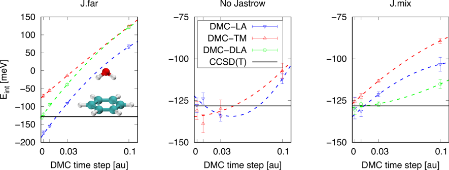
Figure 1: Interaction energy $E_{\text{int}}$ for a water-benzene complex in the so called “2-leg” configuration, for the geometry shown in the inset. The plots show FN-DMC evaluations versus the time-step $\tau$, using LA, TM, and DLA. (Left plot) Results obtained using the Jastrow factor J.far in both the bound and the far configurations. J.far has been optimized for the far configuration, i.e. for non-interacting water-benzene molecules. (Middle plot) Results obtained using a trial wave function without any Jastrow factor. In this case LA and DLA are equivalent. (Right plot) Results obtained with mixed Jastrow factor: for the non-interacting configuration we used J.far, for the bound configuration we used J.bound. The reference CCSD(T) value is $-128\pm 1$ meV.Brandenburg et al. (2019).

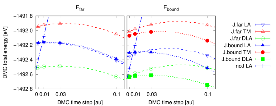
Figure 2: Total energy for the far ($E_{\text{far}}$, left plot) and bound ($E_{\text{bound}}$, right plot) configurations. The plots show FN-DMC evaluations versus the time-step $\tau$, using LA, TM, and DLA, and different choices of the Jastrow factor: J.far, J.bound, and no Jastrow (noJ), as defined in the text. FN-DMC-TM noJ points fall outside the interval range ($E_{\text{far}}=-1491.225(7)$ meV and $E_{\text{bound}}=-1491.358(1)$ meV in the limit $\tau\to 0$).

The left panel of Figure 1 shows results for J.far used for both the bound and the far-away configuration. With this setup DLA is the only method that provides a reliable interaction energy, which we can estimate to be $-131\pm 2$ meV for the $\tau\to 0$ limit from a quadratic fit of the values obtained at finite values of $\tau$. The estimated $\tau\to 0$ limit for LA and TM are $-187\pm 3$ meV and $-76\pm 1$ meV. So, with this non-optimal Jastrow factor LA severely over-binds and TM under-binds.

A different choice, which is indeed the standard procedure adopted in DMC, is to optimize the Jastrow factor specifically for each configuration, i.e. we use J.bound for the bound configuration and J.far for the far configuration. We named this scheme J.mix, and the results obtained with LA, TM, and DLA are shown on the right panel of Figure 1. In this case all three methods are in decent agreement with the CCSD(T) reference, from a quadratic fit we obtain the $\tau\to 0$ limit: $-135\pm 3$ meV for LA, $-127\pm 1$ meV for TM, and $-129\pm 2$ meV for DLA. The figure also shows the time-step error associated with the three different methods. The first consideration is that the better choice of the Jastrow has greatly improved the accuracy for any finite $\tau$ evaluation with respect to the case with J.far. The best time-step dependence is obtained for the DLA approach, where the interaction energy evaluation for $\tau=0.03$ au is $-127\pm 1$ meV, which appears already converged (2 meV difference with respect to the $\tau\to 0$ limit).

At this point one could wonder what is the outcome if the Jastrow is not used at all. We performed the FN-DMC simulation with LA and no Jastrow (so, it is equivalent to DLA), and the outcome is reported on the middle panel of Figure 1. The $\tau\to 0$ limit of the interaction energy is $-125\pm 4$ meV, in excellent agreement with the other DMC-DLA evaluations with J.far and J.mix (as it has to be by construction), and also with the reference CCSD(T). Quite unexpectedly, we also notice that the time-step error is quite small, much smaller than the case with J.far, and similar to the case with J.mix. This happens despite the huge time-step error on the total energy evaluations (see Figure 2) when a Jastrow is not used, and indicates an unexpectedly good error cancellation of the finite step bias in the energy difference. We do not know if this behavior of the no Jastrow case is transferable to other systems. If it was, one would be tempted to do simulations without a Jastrow. However, this is not recommended because the variance of the local energy $\textrm{Var}[E_{L}]$ is much larger without a Jastrow, around ten times the variance of the Slater-Jastrow $\Psi_{T}$. Since the computational cost is proportional to the variance, then a simulation with a given $\tau$ and a target precision will cost, computationally, around an order of magnitude more in the absence of a Jastrow. If this extra cost could be recovered by using time-steps ten times as large is something that would have to be checked on each system.

IV.2 Evaluation of ionization energies

Ionization energies (IEs) are typical quantities that are evaluated when new PPs are developed or tested.Burkatzki et al. (2007); Trail and Needs (2005b, a, 2013, 2015, 2017); Bennett et al. (2017); Annaberdiyev et al. (2018); Krogel et al. (2016); Seth et al. (2011); Fahy et al. (1988); Ertekin et al. (2013) The $n$-th ionization energy IE$(n)$ is the energy necessary to remove one electron from an atomic (or molecular) species $X$ and charge $(n-1)$, i.e. to have $X^{n-1}\to X^{n}+\textrm{e}^{-}$. Good PPs are expected to yield IEs estimations close to the corresponding all-electron (AE) evaluations. Typically these checks are not performed at the QMC level, even for PPs specifically developed for QMC, but using Hartree-Fock, DFT, or CCSD(T). Here, we test the FN-DMC evaluations using LA, TM, and DLA.

We considered the first three ionization energies of the carbon atom, and we performed calculations with the eCEPP pseudopotentialTrail and Needs (2017), which has a He-core for the carbon atom. These pseudopotentials perform very well at the CCSD(T) level of theory. This can be seen in Table 1, where the absolute difference in the IE between AE and eCEPP evaluations is $<0.07$ eV, and the relative difference is $<0.5$%.

Table 1: First three ionization energies of the carbon atom, in eV. We give experimental results (Exp.) and compare CCSD(T) results based on all electron (AE) and PP (eCEPPTrail and Needs (2017)).

	Exp.	AE	eCEPP	$\Delta_{\textrm{eCEPP-AE}}$
IE(1)	11.26	11.26	11.22	-0.04
IE(2)	24.38	24.36	24.29	-0.07
IE(3)	47.89	47.86	47.90	0.04

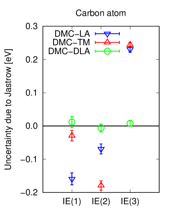
Figure 3: Uncertainty of the FN-DMC estimation of the $n$-th ionization energy IE($n$) of the carbon atom due to the Jastrow, using an eCEPP pseudopotentialTrail and Needs (2017) and either LA, TM, or DLA. Uncertainty is evaluated as the difference between the estimation using two different sets of Slater-Jastrow wave functions having the same ${\cal D}$ and different ${\cal J}$ (see text). Error bars correspond to a standard deviation due to the DMC sampling.

When PPs are deployed in FN-DMC the difference from the AE results can be much larger than what is found for CCSD(T) because of the localization error. As usual, the localization error depends on the trial wave function. To have an idea of the magnitude of the localization error, we performed two sets of FN-DMC calculations, both with eCEPP and a Slater-Jastrow function with the Slater determinant obtained from a DFT/LDA calculation. The difference among the two sets is the Jastrow factor, that in one case (Ju) includes only e-e terms, and in the other case (Juxf) includes e-e, e-n and e-e-n terms. The parameters of the Jastrow factors have been optimized for each atomic ion considered. We have calculated the difference between the FN-DMC evaluations of IE$(n)$ in two sets, for LA, TM, and DLA. Notice that the difference between the corresponding Juxf and the Ju wave functions is solely due to the localization error, because the same ${\cal D}$ is used for Ju and Juxf, so the nodal surfaces are the same. Results are reported on Figure 3. By construction, DLA is not affected by the Jastrow uncertainty, whereas the uncertainty on both TM and LA is larger than 0.2 eV. So, we see in this case that in LA and TM the choice of the Jastrow yields a localization error that can be more than two times larger than the CCSD(T) error of the eCEPP pseudopotential. Given this large uncertainty in LA and TM, it is unclear what the most suitable Jastrow is. Juxf is variationally better than Ju (smaller VMC energy and variance). However, in Appendix D we compare the difference between the PPs and the AE results, and it is unclear if Ju or Juxf is better. DLA solves the issue, because results from Ju and Juxf are equivalent.

In which way can we improve the DMC accuracy with DLA? It can be improved systematically by changing the determinant part, for instance using a multi-determinant ${\cal D}$ term obtained using a method like the complete active space self consistent field (CASSCF),Valsson and Filippi (2010); Zimmerman et al. (2013); Toulouse and Umrigar (2008) the Configuration Interaction using a Perturbative Selection made Iteratively (CIPSI),Giner et al. (2013); Scemama et al. (2018) or the Antisymmetrized Geminal Power.Casula and Sorella (2003); Zen et al. (2014) DLA appears convenient in this case because we can anticipate improvements in the nodes and in the wave function, and we do not need to be concerned about the unpredictable effects of the Jastrow factor.

IV.3 DLA yields stable DMC simulations

Stability is a very important practical aspect of DMC simulations. Instability in DMC is usually correlated with the quality of the trial wave function and of the pseudopotentials. In particular, a possible issue in the trial wave functions, which can generate instability, is the generation of the determinant part ${\cal D}$ of the trial wave function via plane-wave DFT packages using suboptimal Kleinman-Bylander projectors. In QMC (or in DFT calculations using localized basis) the non-local terms in the pseudopotential are evaluated using spherical harmonic projectors. In contrast, in plane-wave DFT calculations the non-local terms in the pseudopotential are evaluated using Kleinman-Bylander projectorsKleinman and Bylander (1982) (i.e. projected into pseudo-atom wave functions). Thus, there is a possible inconsistency between the projection of the non-local terms at the DFT and DMC levels. The inconsistency is even worse if the Kleinman-Bylander projectors are not obtained with the same DFT functional used in the DFT preparation of ${\cal D}$. As a consequence, the method adopted to deal with the non-local part of the pseudopotential (LA, TM, or DLA) has a big impact on the stability of the DMC simulation. We have observed that DLA is not affected by the instability issues of LA, and in all test simulations is as stable as TM and more stable than LA.

To illustrate this point, we consider carbon dioxide, CO₂, because in a previous studyZen et al. (2018) we noticed that the CO₂ molecule often leads to unstable DMC simulations. We consider here the case of the monomer and dimer of CO₂ (configurations taken from Ref. Zen et al., 2018) and we use CEPP pseudopotentialsTrail and Needs (2013) for both oxygen and carbon. We obtain ${\cal D}$ from a DFT/LDA calculation using the PWSCF codeGiannozzi et al. (2009), with a 600 Ry plane wave cutoff, and the molecular orbitals obtained were converted into splinesAlfè and Gillan (2004). The Kleinman-Bylander projectors used in DFT are from Ref. Trail and Needs, 2013, and they were obtained from DFT/PBE so there is an inconsistency with the employed DFT functional. In QMC, we used a Jastrow factor ${\cal J}$ with e-e, e-n and e-e-n terms, and parameters were optimized by minimizing the local energy variance in VMC yielding $\textrm{Var}[E_{L}]_{\text{VMC}}=0.956(2)$ au in the molecule. The same identical trial wave function (i.e., no other optimization of ${\cal J}$) has a much smaller local energy variance in VMC if the DLA local energy $E_{L}^{DLA}$ (as obtained from the Hamiltonian given in Eq. 14) is used: $\textrm{Var}[E_{L}^{DLA}]_{\text{VMC}}=0.685(5)$ au. Thus, the DLA Hamiltonian might already have advantages at the VMC level.

At the DMC level LA simulations are not possible, as population explosions happens so frequently that it was not possible to finish the DMC equilibration. In contrast, both TM and DLA yield stable DMC simulations at all the attempted time-steps (0.03, 0.01 and 0.003 au). Moreover, the results of the DMC simulations seem reasonable despite the issue in the wave function. The most interesting quantity to consider is the interaction energy $E_{\text{int}}$. In this case, as the two carbon dioxide molecules are identical, the interaction can be evaluated as $E_{\text{int}}=E_{\text{dimer}}-2*E_{\text{monomer}}$, the difference between the energy of the dimer and twice the energy of the monomer. The FN-DMC results with TM and DLA are reported in Figure 4. Both methods are in good agreement with the reference CCSD(T) evaluationZen et al. (2018) when we consider the infinitesimal time-step limit. DMC-DLA is less affected by finite time-step bias than DMC-TM. This is probably a consequence of the fact that the local energy variance in DLA is smaller than in TM.

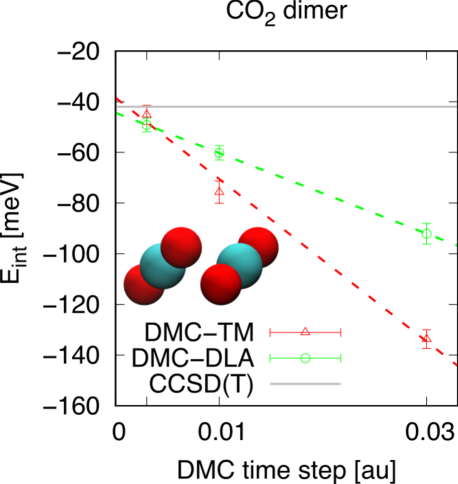
Figure 4: Carbon dioxide dimer configuration (inset) and interaction energy $E_{\text{int}}$ obtained from FN-DMC calculations and plotted as a function of the DMC time-step $\tau$. Dashed lines are obtained from a linear fit, and the extrapolated $\tau\to 0$ values are -38(5) meV and -44(1) meV for TM and DLA, respectively. The reference CCSD(T) value is -42 meV.Zen et al. (2018) DMC-LA is not reported because the simulations are unstable.

IV.4 Good efficiency for DLA

Efficiency is a fundamental property of a computational method. DLA appears to be more efficient than LA and TM. The efficiency of DMC can be estimated, as detailed in Appendix E. The choice among LA, TM, and DLA influences two quantities affecting the DMC efficiency: the computational cost $T_{\text{step}}$ for a single DMC time-step, and the variance $\sigma_{\text{sys}}^{2}$ of the local energy. The most efficient methods will have smaller $T_{\text{step}}$ and $\sigma_{\text{sys}}^{2}$. DLA satisfies both the conditions. A detailed comparison of the efficiency of LA, TM, and DLA is provided in Appendix E. The outcome is that DLA is more efficient in most of the simulations involving organic molecules by roughly 30%.

V Conclusion

In this paper we have illustrated some drawbacks of FN-DMC in the presence of pseudopotentials. Specifically: (i) They generate unpredictable differences on results as a consequence of some arbitrary choices on the Jastrow functional form and the stochastic optimization procedure; (ii) They might affect the reproducibility of results if different QMC packages are used; (iii) The accuracy deteriorates whenever the Jastrow factor is not good, which is not easy to establish. These issues are particularly problematic for precisely where FN-DMC is most needed and offers most promise. We have shown that these issues arise essentially because the pseudopotentials have non-local terms. Within both LA and TM, the projection scheme is affected by a subtle interaction between the Jastrow factor and the pseudopotentials. In this paper we have introduced a new alternative approximation, called the DLA. When FN-DMC deploys DLA the projected wave function and the associated energy are not affected by the Jastrow factor. This solves the mentioned drawbacks. The advantages of DLA have been illustrated on a few examples, including the evaluation of an interaction energy and ionization energies. Moreover, the proposed algorithm appears as stable as TM and is much more stable than LA. In terms of efficiency, DLA performs better than both LA and TM.

An interesting perspective for DLA is that it allows the development of general purpose Jastrow factors, which do not need a system dependent optimization and yield a validated accuracy. In this way, DLA opens the way to the automation of the FN-DMC, which can make DMC easier and less labour intense to use.

The DLA method is already implemented in the CASINONeeds et al. (2010), TurboRVBTur , and QMCPACKKim et al. (2018) packages.

Appendix A DMC implementation and Fixed-Node approximation

In DMC the non-negative and normalized function $f({\bf R},t)$ is interpreted as a probability density distribution, which is represented at each time $t$ via a large number of electronic configurations ${\bf R}_{i}(t)$, also called walkers, and their associated weights $w_{i}(t)$. Walkers ${\bf R}_{i}(t)$ and weights $w_{i}(t)$ evolve in time according to a process that is ultimately determined by the Green’s function.Foulkes et al. (2001) A key issue is that the Green’s function $G({\bf R}^{\prime}\leftarrow{\bf R},t)$ in eq. (4) does not impose any anti-symmetry constraint to the system, so the ground state $\Phi$ obtained according to the imaginary time projection in eq. (5) would be bosonic, as it has a lower energy than the corresponding fermionic system. The traditional and most effective way to impose anti-symmetry in $\Phi$ is to adopt the fixed node (FN) approximation: walkers are not allowed to cross the nodal surface of the trial wave function $\Psi_{T}({\bf R})$. In other terms, the Hamiltonian $\hat{H}$ is replaced by the FN Hamiltonian $\hat{H}_{FN}\equiv\hat{H}+\hat{V}_{FN}\,,$ where $\hat{V}_{FN}$ is an infinite wall at the nodal surface of $\Psi_{T}$. The projected function $\Phi_{FN}({\bf R})$ obtained in this way has the same nodes as $\Psi_{T}({\bf R})$, and it is the exact solution for the Hamiltonian $\hat{H}_{FN}$, namely $\hat{H}_{FN}\left|\Phi_{FN}\right>=E_{FN}\left|\Phi_{FN}\right>$. This implies that $E_{FN}={\left<\Phi_{FN}\right|\hat{H}_{FN}\left|\Psi_{T}\right>\over\left<\Phi_{FN}\middle|\Psi_{T}\right>}$, and noticing that $\hat{H}_{FN}\left|\Psi_{T}\right>=\hat{H}\left|\Psi_{T}\right>$ because $\hat{V}_{FN}\neq 0$ only in the nodal surface of $\Psi_{T}$, so we can evaluate $E_{FN}$ using the mixed estimator:

$$E_{FN}={\int\Phi_{FN}({\bf R})\Psi_{T}({\bf R})E_{L}({\bf R})d{\bf R}\over\int\Phi_{FN}({\bf R})\Psi_{T}({\bf R})d{\bf R}}\,.$$ (16)

The FN energy $E_{FN}$ is an upper bound to the exact energy $E_{0}$, namely $E_{FN}\geq E_{0}\,,$ because $\hat{H}_{FN}\geq\hat{H}$. The approach is exact if the nodes of $\Psi_{T}({\bf R})$ are exact, because in this case $\hat{H}_{FN}\left|\Phi_{FN}\right>=\hat{H}\left|\Phi_{FN}\right>$. Thus, the quality of the FN approximation is determined by the quality of the nodes of the trial function $\Psi_{T}({\bf R})$.

Appendix B Hamiltonian for all-electrons versus Hamiltonian for valence electrons and pseudopotentials

The electronic Hamiltonian in Born-Oppenheimer approximation is:

$$\hat{H}=-{1\over 2}\sum_{i}^{N}\nabla_{i}^{2}+\sum_{i<j}^{N}{1\over r_{ij}}-\sum_{i}^{N}\sum_{\alpha}^{M}{Z_{\alpha}\over r_{i\alpha}}$$ (17)

where roman letters are used to label the $N$ electrons and greek letters to label the $M$ ions; $r_{ij}=|{\bf r}_{i}-{\bf r}_{j}|$ is the distance between electrons $i$ and $j$; $r_{i\alpha}=|{\bf r}_{i}-{\bf r}_{\alpha}|$ is the distance between electron $i$ and ion $\alpha$. The first term in the right hand size is the kinetic energy $\hat{K}$ and the other two terms define a local potential $\hat{V}_{L}$.

The electrons can be separated into $N_{c}$ core and $N_{v}$ valence electrons, such that $N=N_{v}+N_{c}$. Thus, equation (17) can be recasted to:

$$\hat{H} = \hat{H}_{v}+\hat{H}_{c}+\hat{H}_{cv}$$ (18)

$$\hat{H}_{v} = -{1\over 2}\sum_{i}^{N_{v}}\nabla_{i}^{2}+\sum_{i<j}^{N_{v}}{1\over r_{ij}}-\sum_{i}^{N_{v}}\sum_{\alpha}^{M}{Z_{\alpha}\over r_{i\alpha}}$$ (19)

$$\hat{H}_{c} = -{1\over 2}\sum_{i}^{N_{c}}\nabla_{i}^{2}+\sum_{i<j}^{N_{c}}{1\over r_{ij}}-\sum_{i}^{N_{c}}\sum_{\alpha}^{M}{Z_{\alpha}\over r_{i\alpha}}$$ (20)

$$\hat{H}_{cv} = +\sum_{i}^{N_{c}}\sum_{j}^{N_{v}}{1\over r_{ij}}$$ (21)

where $\hat{H}_{v}$ and $\hat{H}_{c}$ are the components of the Hamiltonian involving only the valence electrons and the core electrons, respectively, and $\hat{H}_{cv}$ is the explicit pairing interaction between the core and the valence electrons.

All electron calculations in QMC are computationally very expensive, having a scaling roughly proportional to $Z_{\alpha}^{6}$,Ceperley (1986); Hammond et al. (1987); Ma et al. (2005) because close to the nucleus the local energy has large fluctuations, yielding a large variance and thus requiring very small time-steps. As many properties of interest are determined by the behavior of the valence electrons, it is often convenient to use pseudopotentials to represent the core electrons, especially in heavy nuclei. The Hamiltonian for calculations with pseudopotentials is then of the following:

$$\hat{H}_{\text{PP}}=-{1\over 2}\sum_{i}^{N_{v}}\nabla_{i}^{2}+\sum_{i<j}^{N_{v}}{1\over r_{ij}}+\sum_{i}^{N_{v}}\sum_{\alpha}^{M}\hat{V}_{\text{PP}}^{\alpha}({\bf r}_{i})$$ (22)

where the first two terms in the RHS are the kinetic and electron-electron interactions, respectively, as expressed also in $\hat{H}_{v}$. The interaction between electron $i$ and ion $\alpha$ are described as follows:

$$\hat{V}_{\text{PP}}^{\alpha}({\bf r}_{i})=V_{\text{loc}}^{\alpha}(r_{i\alpha})+\sum_{l=0}^{l_{\text{max}}}V_{l}^{\alpha}(r_{i\alpha})\hat{P}_{l}^{\alpha}$$ (23)

where $V_{\text{loc}}^{\alpha}(r_{i\alpha})$ is the local part of the pseudopotential of ion $\alpha$, and $V_{l}^{\alpha}(r_{i\alpha})$ are the non-local components, which are applied via the projector:

$$\hat{P}_{l}^{\alpha}=\sum_{m=-l}^{+l}\left|Y^{\alpha}_{l,m}\middle>\middle<Y^{\alpha}_{l,m}\right|$$

where $\left|Y^{\alpha}_{l,m}\right>$ are spherical harmonics centered on nucleus $\alpha$. The idea behind $\hat{V}_{\text{PP}}^{\alpha}({\bf r}_{i})$ is that it represents an effective potential that reproduces the effects of both the nucleus and the core electrons on the valence electrons. However, there is not an exact mapping, or a thermodynamic integration, providing the pseudopotentials. Indeed some criteria needs to be chosen to produce them, and they need to be tested at some level of theory. Moreover, it has to be noticed that in independent-electron theories, such as HF and DFT, the separation of the electrons among core and valence can be in principle exact, while it cannot be exact in QMC or in other many-body approaches, because of the electronic correlation. Thus, although the employment of pseudopotentials in QMC is most of the times necessary for efficiency reasons, it can yield errors which cannot be easily quantified. Accurate pseudopotentials for QMC are so far available only for a fraction of the periodic table. The few cases where QMC proves less accurate than DFT are typically related with poor quality PPs used in QMC.Saritas et al. (2017) A crucial property of a PP is its transferability, which is affected by the range of the non-local potential terms (the smaller the better) and the inclusion of higher angular momentum channels.Tipton et al. (2014)

Appendix C Jastrow interaction with pseudopotential non-local term

In sections II.4.1 and II.4.2 we have shown that the non-local operators needs to be localized using the trial wave function $\Psi_{T}$, such that the localized non-local operator ${\hat{V}_{NL}\Psi_{T}\over\Psi_{T}}$ acts on a generic function $\xi({\bf R})$ as follows:

$${\hat{V}_{NL}\Psi_{T}\over\Psi_{T}}\xi({\bf R})={\cal V}_{NL}^{loc}({\bf R})\xi({\bf R})\,.$$

By using the addition theorem for spherical harmonics and equations 22 and 23, it can be shown that ${\cal V}_{NL}^{loc}({\bf R})$ can be evaluated as follows:

$${\cal V}_{NL}^{loc}({\bf R})=\sum_{i}^{N_{v}}\sum_{\alpha}^{M}\sum_{l=0}^{l_{\text{max}}}{2l+1\over 4\pi}V_{l}^{\alpha}(r_{i\alpha})\int P_{l}(\cos\theta^{\prime}_{i\alpha}){\Psi_{T}({\bf r}_{1},\ldots,{\bf r}_{i-1},{\bf r^{\prime}}_{i},{\bf r}_{i+1}\ldots,{\bf r}_{N_{v}})\over\Psi_{T}({\bf r}_{1},\ldots,{\bf r}_{N_{v}})}d\Omega^{\prime}_{i\alpha}$$ (24)

where the angular integration is over the sphere passing through the $i$-th electron and centered on the $\alpha$-th atom, $P_{l}$ is the Legendre polynomial of degree $l$, and $\cos\theta^{\prime}_{i\alpha}={{\bf r}^{\prime}_{i\alpha}\cdot{\bf r}_{i\alpha}\over r^{\prime}_{i\alpha}r_{i\alpha}}$.

Therefore, in the evaluation of ${\cal V}_{NL}^{loc}({\bf R})$ we have to integrate the ratio between the trial wave functions for electrons displaced along spheres centered on every pseudo-atom. By considering that $\Psi_{T}={\cal D}*\exp{\cal J}$, it is clear that this ratio has to be taken for both the determinant part ${\cal D}$ and the Jastrow factor $\exp{\cal J}$. This expression explains why both LA and TM yield to total energies that depend on the Jastrow factor: ${\cal J}$ effectively changes the potential term in the effective Hamiltonian, due to the localization of the non-local term.

We could wonder what parts of the Jastrow factor give rise to this issue, and if it is possible to use a Jastrow not affecting the ratio in the RHS of equation 24. Although there are differences in the Jastrow factor implemented in the different codes, they typically can be expressed in the following way:

$${\cal J}({\bf R})=\sum_{i<j}\delta_{\sigma_{i},\sigma_{j}}u_{\uparrow\uparrow}(r_{ij})+\sum_{i<j}(1-\delta_{\sigma_{i},\sigma_{j}})u_{\uparrow\downarrow}(r_{ij})+\sum_{\alpha}\sum_{i}\chi_{\alpha}(r_{i\alpha})+\sum_{\alpha}\sum_{i<j}f_{\alpha}(r_{i\alpha},r_{j\alpha},r_{ij})$$ (25)

where $u_{\uparrow\uparrow}$ and $u_{\uparrow\downarrow}$ are homogeneous two-electron correlation terms, or e-e, describing the interation between like-spin and unlike-spin pairs, $\chi_{\alpha}$ is a e-n term depending on the distance of any electron from the $\alpha$-th atom, and $f_{\alpha}$ is a three-body term, or e-e-n, describing the interaction between electron pairs in proximity of the $\alpha$-th atom. Different packages can provide different parametrization of these terms, and sometimes additional terms. The important aspect is that in the displacement ${\bf r}_{i}\to{\bf r}^{\prime}_{i}$ performed in the angular integration in equation 24, we have that $r_{i\alpha}\to r^{\prime}_{i\alpha}=r_{i\alpha}$ but $r_{ij}\to r^{\prime}_{ij}\neq r_{ij}$. Thus, the e-n term $\chi_{\alpha}$ is not responsible for the Jastrow dependence of ${\cal V}_{NL}^{loc}({\bf R})$, while the e-e and e-e-n terms are at the source of the issue. One could in principle decide to do not use the three-body term $f_{\alpha}$, but the same cannot be done for the terms $u_{\uparrow\uparrow}$ and $u_{\uparrow\downarrow}$, as they are the most important in the Jastrow factor, responsible for most of the correlation captured by $\Psi_{T}$ and the decrease in the variance of the local energy.Grüneis et al. (2017)

Appendix D How large are errors due to PPs in IE evaluations?

Ideally, a perfect PP delivers exactly the same energy differences as AE calculations. In FN-DMC the situation is complicated by the fact that localization errors appear when PPs are used. In section IV.2 it is shown that these localization errors can be large, and that with LA and TM there is a big dependence on the Jastrow factor in the trial wave function. For instance, it is not clear if both the wave functions Ju and Juxf discussed in section IV.2 show a sizable localization error, or if instead one wave function is responsible for most of the error.

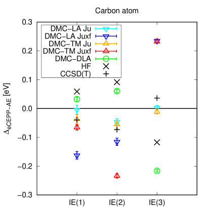
Figure 5: Difference $\Delta_{\text{eCEPP-AE}}$ between the IE$(n)$ evaluation with eCEPP PPs and with all-electrons (AE). FN-DMC with PPs yields different results with different $\Psi_{T}$, and we consider two sets of Slater-Jastrow functions, dubbed Ju and Juxf (see text). In all reported DMC calculations, ${\cal D}$ is a single Slater determinant obtained from DFT/LDA. Results using LA, TM, and DLA are shown. As a comparison, outcomes from Hartree Fock (HF) and CCSD(T) are also reported.

In order to investigate this, we have considered the difference $\Delta_{\text{eCEPP-AE}}$ between the eCEPP and the AE results, the IE$(n)$ evaluated with LA, TM and DLA. In the AE calculation we have used the same level of theory to generate the wave function, so a Slater-Jastrow function with the determinant from DFT/LDA. Results are reported in Figure 5. The plot highlights some unexpected behavior. We would have expected that the Juxf yields better results than Ju, because Juxf has more parameters and include Ju as a special case, and indeed it yields a lower variational energy and variance than Ju. However, Juxf does not show a smaller $\Delta_{\text{eCEPP-AE}}$ compared to Ju in any of the IEs. In fact, the worse wave function, Ju, generates the smallest $\Delta_{\text{eCEPP-AE}}$ in LA and TM. On the other hand, DLA yields $\Delta_{\text{eCEPP-AE}}$ quite similar in absolute value to the best LA or TM case, but in DLA the sign is inverted. We notice a clear correlation between DLA and HF errors. This correlation suggests that the $\Delta_{\text{eCEPP-AE}}$ in DLA might just reflect the limitations of the determinant part of the wave function.

Appendix E Estimation of computational cost of a FN-DMC simulation with LA, TM, and DLA

The efficiency of a DMC calculation depends on the computational resources required to achieve a target stochastic error $\sigma_{\text{target}}$ on the quantity of interest. In most cases we are interested in the energy, and in this case the computational time spent $T_{\text{cost}}$ is

$$T_{\text{cost}}=T_{\text{step}}*{t_{\text{ac}}\over\tau}\left({t_{\text{ac}}\over t_{\text{eq}}}N_{w}+{\sigma_{\text{sys}}^{2}\over\sigma_{\text{target}}^{2}}\right)\,,$$ (26)

where $T_{\text{step}}$ is the computational time of a single DMC step (which clearly depends on the specific architecture where the calculation is performed), $t_{\text{ac}}$ and $t_{\text{eq}}$ are the autocorrelation and equilibration times (which are roughly the same and typically of the order of 1 au), $N_{w}$ is the number of walkers, and $\sigma_{\text{sys}}^{2}$ is the variance of the local energy in the corresponding DMC scheme. The first term into the parenthesis is due to the equilibration time in DMC, which has to be removed from the sampling, and that typically is negligible compared to the second term into the parenthesis, which instead comes from the statistical sampling. The quantities on the RHS of eq. (26) that are affected by the choice of LA, TM or DLA are only $T_{\text{step}}$ and $\sigma_{\text{sys}}^{2}$. In particular, $\sigma_{\text{sys}}^{2}$ is $\textrm{Var}[E_{L}]_{\text{DMC-LA}}$, $\textrm{Var}[E_{L}]_{\text{DMC-TM}}$, and $\textrm{Var}[E_{L}^{DLA}]_{\text{DMC-DLA}}$ for LA, TM, and DLA, respectively.

The dependence on $T_{\text{step}}$ is straightforward: if we name $T_{\text{step}}^{LA}$, $T_{\text{step}}^{TM}$ and $T_{\text{step}}^{DLA}$ the cost per step in the LA, TM and DLA approaches, respectively, then

$$T_{\text{step}}^{DLA}<T_{\text{step}}^{LA}<T_{\text{step}}^{TM}\,.$$

Indeed, in TM the operations are just the same performed in LA, plus those to perform the moves connected to the Green’s function $T_{NL}({\bf R}^{\prime}\leftarrow{\bf R})$ (T-moves). On the other hand, in DLA there are fewer operations than in LA because the Jastrow factor does not need to be considered when evaluating the non-local part of the pseudopotential (see details in Appendix C). However, the observed difference in the costs of LA, TM and DLA is relatively small (just a few percent).

More important for the efficiency is the dependence on the variance $\sigma_{\text{sys}}^{2}$. First of all, we have to notice that here the variance under consideration is the one relative to the corresponding DMC sampling, which is $\textrm{Var}[E_{L}]_{\text{DMC-LA}}$, $\textrm{Var}[E_{L}]_{\text{DMC-TM}}$, and $\textrm{Var}[E_{L}^{DLA}]_{\text{DMC-DLA}}$ for LA, TM and DLA, respectively. The LA and TM approaches are strictly related with the variational variance $\textrm{Var}[E_{L}]_{\text{VMC}}$; the local energy is calculated in the same way but the underlying probability distribution is different, and in particular different values of the time-step change the sampling and the corresponding variance. In DMC-LA with large $\tau$ the variance becomes the same as the variational variance (this is likely a consequence of the Metropolis step to enforce detailed balance after the drift-diffusion step), while at small $\tau$ we notice that the DMC-LA variance is typically slightly smaller than the VMC variance. In DMC-TM the variance converges to the same variance of DMC-LA for small $\tau$, but for large $\tau$ it is larger than the VMC and the DMC-LA variance. In DMC-DLA the variance has roughly the same relation with the variational DLA variance that the DMC-LA variance has with the VMC variance. Thus, the difference in the variance between DMC-LA and DMC-DLA is mostly captured by the difference in the corresponding variational variances, $\textrm{Var}[E_{L}]_{\text{VMC}}$ and $\textrm{Var}[E_{L}^{DLA}]_{\text{VMC}}$. Notice that the VMC sampling is precisely the same if $\Psi_{T}$ is the same, and the difference only comes from the Hamiltonian, thus the local energy.

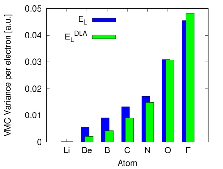
Figure 6: Local energy variances in VMC, $\textrm{Var}[E_{L}]_{\text{VMC}}$ in blue and $\textrm{Var}[E_{L}^{DLA}]_{\text{VMC}}$ in green, per valence electron on the first-row atoms, using eCEPP pseudopotentialsTrail and Needs (2017) (He-core), a Jastrow factor with e-e, e-n and e-e-n terms, and a single Slater determinant obtained from a DFT/LDA calculation with the aug-cc-pVQZ-eCEPP basis.Trail and Needs (2017)

In order to investigate this difference, in Figure 6 we report the variational variances ($\textrm{Var}[E_{L}]_{\text{VMC}}$ and $\textrm{Var}[E_{L}^{DLA}]_{\text{VMC}}$) per electron on the first-row atoms, using eCEPP pseudopotentialsTrail and Needs (2017), which are He-core for all the reported atoms. The ${\cal D}$ in $\Psi_{T}$ was obtained from a DFT/LDA calculation performed with the Orca packageNeese (2012) and with the localized basis set aug-cc-pVQZ-eCEPP provided in Ref. Trail and Needs, 2017. The Jastrow factor used has e-e, e-n and e-e-n terms, with parameters optimized in any atom to minimize the variational variance. Figure 6 shows that $\textrm{Var}[E_{L}^{DLA}]_{\text{VMC}}$ is smaller than $\textrm{Var}[E_{L}]_{\text{VMC}}$ for most elements with the exception of the fluorine atom where the DLA variance is +6% larger. In particular, in the carbon atom the variance is -32% smaller, in the nitrogen atom is -13%, in oxygen atom in -0.5%.

A natural question at this point is: which part of ${\cal J}$ is mostly involved in producing a difference between $E_{L}$ and $E_{L}^{DLA}$? In Appendix C we show that the e-n term drops out when we evaluate the non-local potential term, thus it produces no difference between $E_{L}$ and $E_{L}^{DLA}$. The terms to consider are thus the e-e and the e-e-n. In Table 2 we report the variational variances on the boron atom with different parametrizations of the ${\cal J}$. It shows than the e-e term produces most of the difference. Moreover, one could wonder how much this difference is affected by the choice of the pseudopotentials. In Table 2 we provide the variance also for the ccECP pseudopotentialBennett et al. (2017). We notice that, despite in absolute terms eCEPP and ccECP yield different variances, in relative terms the difference between $E_{L}$ and $E_{L}^{DLA}$ is the same.

Table 2: Variational variance, in au, $\textrm{Var}[E_{L}]_{\text{VMC}}$ and $\textrm{Var}[E_{L}^{DLA}]_{\text{VMC}}$ for the boron atom, simulated using He-core pseudopotentials, a single Slater determinant obtained from a DFT/LDA calculation and different parametrizations of the Jastrow factor ${\cal J}$, each with parameters optimized to minimize the variance. For the eCEPP pseudopotentialsTrail and Needs (2017) we used the aug-cc-pVQZ-eCEPP basis provided by Trail and Needs (2017), while for the ccECP pseudopotentialsBennett et al. (2017) we used the QZ basis provided by Bennett et al. (2017).

Pseudo	Jastrow	$\textrm{Var}[E_{L}]_{\text{VMC}}$	$\textrm{Var}[E_{L}^{DLA}]_{\text{VMC}}$
eCEPP	no	0.181(3)	0.181(3)
eCEPP	e-e	0.0401(1)	0.0317(1)
eCEPP	e-e, e-n	0.0285(3)	0.0135(1)
eCEPP	e-e, e-n, e-e-n	0.0278(2)	0.0133(1)
ccECP	e-e, e-n, e-e-n	0.0355(4)	0.0166(1)

The lower variance automatically translates into a smaller stochastic error in the DMC evaluations with same sampling. Thus, DLA is more efficient in most of the simulations involving organic molecules, because they are characterized by the presence of many carbon atoms, where DLA is roughly 30% faster than LA and even more compared to TM (where it crucially depends on the time-step value).

References

- Foulkes et al. (2001) W. M. C. Foulkes, L. Mitas, R. J. Needs, and G. Rajagopal, Rev. Mod. Phys. 73, 33 (2001).
- Zen et al. (2018) A. Zen, J. G. Brandenburg, J. Klimeš, A. Tkatchenko, D. Alfè, and A. Michaelides, P. Natl. Acad. Sci. Usa 115, 1724 (2018).
- Brandenburg et al. (2019) J. G. Brandenburg, A. Zen, M. Fitzner, B. Ramberger, G. Kresse, T. Tsatsoulis, A. Grüneis, A. Michaelides, and D. Alfè, J. Phys. Chem. Lett. 10, 358 (2019).
- Zen et al. (2016a) A. Zen, L. M. Roch, S. J. Cox, X. L. Hu, S. Sorella, D. Alfè, and A. Michaelides, J. Phys. Chem. C 120, 26402 (2016a).
- Al-Hamdani et al. (2017a) Y. S. Al-Hamdani, M. Rossi, D. Alfè, T. Tsatsoulis, B. Ramberger, J. G. Brandenburg, A. Zen, G. Kresse, A. Grüneis, A. Tkatchenko, and A. Michaelides, J. Chem. Phys. 147, 044710 (2017a).
- Al-Hamdani et al. (2017b) Y. S. Al-Hamdani, D. Alfè, and A. Michaelides, J. Chem. Phys. 146, 094701 (2017b).
- Al-Hamdani et al. (2015) Y. S. Al-Hamdani, M. Ma, D. Alfè, O. A. von Lilienfeld, and A. Michaelides, J. Chem. Phys. 142, 181101 (2015).
- Trail et al. (2017) J. Trail, B. Monserrat, P. López Ríos, R. Maezono, and R. J. Needs, Phys. Rev. B 95, 77 (2017).
- Luo et al. (2017) Y. Luo, A. Benali, L. Shulenburger, J. T. Krogel, O. Heinonen, and P. R. C. Kent, New J. Phys. 18, 1 (2017).
- Dubecký et al. (2016) M. Dubecký, L. Mitas, and P. Jurecka, Chem. Rev. 116, 5188 (2016).
- Devaux et al. (2015) N. Devaux, M. Casula, F. Decremps, and S. Sorella, Phys. Rev. B 91, 081101 (2015).
- Wu et al. (2015) Y. Wu, L. K. Wagner, and N. R. Aluru, J. Chem. Phys. 142, 234702 (2015).
- Zheng and Wagner (2015) H. Zheng and L. K. Wagner, Phys. Rev. Lett. 114, 176401 (2015).
- Wagner and Abbamonte (2014) L. K. Wagner and P. Abbamonte, Phys. Rev. B 90, 125129 (2014).
- Azadi et al. (2014) S. Azadi, B. Monserrat, W. M. C. Foulkes, and R. J. Needs, Phys. Rev. Lett. 112, 609 (2014).
- Benali et al. (2016) A. Benali, L. Shulenburger, J. T. Krogel, X. Zhong, P. R. C. Kent, and O. Heinonen, Phys. Chem. Chem. Phys. 18, 18323 (2016).
- Shin et al. (2017) H. Shin, Y. Luo, P. Ganesh, J. Balachandran, J. T. Krogel, P. R. C. Kent, A. Benali, and O. Heinonen, Phys. Rev. Materials 1, 073603 (2017).
- Ahn et al. (2018) J. Ahn, I. Hong, Y. Kwon, R. C. Clay, L. Shulenburger, H. Shin, and A. Benali, Phys. Rev. B 98, 085429 (2018).
- Tsatsoulis et al. (2017) T. Tsatsoulis, F. Hummel, D. Usvyat, M. Sch tz, G. H. Booth, S. S. Binnie, M. J. Gillan, D. Alf, A. Michaelides, and A. Gr neis, J. Chem. Phys. 146, 204108 (2017).
- Doblhoff-Dier et al. (2017) K. Doblhoff-Dier, J. Meyer, P. E. Hoggan, and G.-J. Kroes, J. Chem. Theory Comput. 13, 3208 (2017).
- Maurer et al. (2019) R. J. Maurer, C. Freysoldt, A. M. Reilly, J. G. Brandenburg, O. T. Hofmann, T. Björkman, S. Lebègue, and A. Tkatchenko, Annu. Rev. Mater. Res. 49, 3.1 (2019).
- Note (1) Alternative strategies to the FN approximation have been developed,Ceperley and Alder (1984); Bianchi et al. (1993); Arnow et al. (1982); Anderson et al. (1991); Zhang and Kalos (1991); Kalos and Pederiva (2000); Reboredo et al. (2009) which are typically more accurate but much more demanding in terms of computational cost. Thus, typically only FN-DMC is affordable in large systems.
- Ceperley (1986) D. M. Ceperley, Journal Of Statistical Physics 43, 815 (1986).
- Hammond et al. (1987) B. L. Hammond, P. J. Reynolds, and W. A. Lester, J. Chem. Phys. 87, 1130 (1987).
- Ma et al. (2005) A. Ma, N. D. Drummond, M. D. Towler, and R. J. Needs, Phys. Rev. E 71, 283 (2005).
- Zen et al. (2016b) A. Zen, S. Sorella, M. J. Gillan, A. Michaelides, and D. Alfè, Phys. Rev. B 93, 241118 (2016b).
- Umrigar et al. (1993) C. J. Umrigar, M. P. Nightingale, and K. J. Runge, J. Chem. Phys. 99, 2865 (1993).
- DePasquale et al. (1988) M. F. DePasquale, S. M. Rothstein, and J. Vrbik, J. Chem. Phys. 89, 3629 (1988).
- Casula (2006) M. Casula, Physical Review B 74, 161102 (2006).
- Mitas et al. (1991) L. Mitas, E. L. Shirley, and D. M. Ceperley, J. Chem. Phys. 95, 3467 (1991).
- Casula et al. (2010) M. Casula, S. Moroni, S. Sorella, and C. Filippi, J. Chem. Phys. 132, 154113 (2010).
- Note (2) The localization error goes to zero (ideally) as we can find a closer to the (unknown) fixed-node solution , both in LA and TM.
- Note (3) TM yields more stable simulations than LA.Casula (2006); Drummond et al. (2016) However, if the trial wave function is good LA has typically no stability issues. In these cases TM is often affected by larger finite time-step and stochastic errors than LA.Pozzo and Alfè (2008) Moreover, LA satisfies a detailed balance condition while TM does not, and the size-consistency condition can be harder to satisfy in TM (indeed, the first version of the TM algorithmCasula (2006) was size-inconsistent, an issue solved four years later with two alternative revised TM algorithmsCasula et al. (2010)). Recent investigationsKrogel and Kent (2017); Dzubak et al. (2017) of the localization errors in LA and TM do not show that one method is clearly superior to the other in terms of accuracy.
- Filippi and Umrigar (1996) C. Filippi and C. J. Umrigar, J. Chem. Phys. 105, 213 (1996).
- Valsson and Filippi (2010) O. Valsson and C. Filippi, J. Chem. Theory Comput. 6, 1275 (2010).
- Zimmerman et al. (2013) P. M. Zimmerman, J. Toulouse, Z. Zhang, C. B. Musgrave, and C. J. Umrigar, J. Chem. Phys. 131, 124103 (2013).
- Toulouse and Umrigar (2008) J. Toulouse and C. J. Umrigar, J. Chem. Phys. 128, 174101 (2008).
- Giner et al. (2013) E. Giner, A. Scemama, and M. Caffarel, Can. J. Chem. 91, 879 (2013).
- Scemama et al. (2018) A. Scemama, Y. Garniron, M. Caffarel, and P.-F. Loos, J. Chem. Theory Comput. 14, 1395 (2018).
- Braida et al. (2011) B. Braida, J. Toulouse, M. Caffarel, and C. J. Umrigar, The Journal of Chemical Physics 134, 084108 (2011).
- Casula and Sorella (2003) M. Casula and S. Sorella, J. Chem. Phys. 119, 6500 (2003).
- Zen et al. (2014) A. Zen, E. Coccia, Y. Luo, S. Sorella, and L. Guidoni, J. Chem. Theory Comput. 10, 1048 (2014).
- Bajdich et al. (2006) M. Bajdich, L. Mitas, G. Drobny, L. Wagner, and K. Schmidt, Phys. Rev. Lett. 96, 130201 (2006).
- Austin et al. (2012) B. M. Austin, D. Y. Zubarev, and W. A. J. Lester, Chem. Rev. 112, 263 (2012).
- Feynman and Cohen (1956) R. Feynman and M. Cohen, Phys. Rev. 102, 1189 (1956).
- López Ríos et al. (2006) P. López Ríos, A. Ma, N. D. Drummond, M. D. Towler, and R. J. Needs, Phys. Rev. E 74, 066701 (2006).
- Holzmann and Moroni (2019) M. Holzmann and S. Moroni, Phys. Rev. B 99, 085121 (2019).
- Hammond et al. (1994) B. L. Hammond, W. A. Lester, and P. J. Reynolds, Monte Carlo Methods in Ab Initio Quantum Chemistry (WORLD SCIENTIFIC, 1994) https://www.worldscientific.com/doi/pdf/10.1142/1170 .
- Kalos and Whitlock (2009) M. H. Kalos and P. A. Whitlock, Monte Carlo Methods, 1st ed. (Wiley, 2009).
- Note (4) Given the values of and , we can approximate where , , and .
- Note (5) For instance, it has been observed that the time-step error is largely decreased if a Metropolis step is included in order to enforce detailed balanceCeperley et al. (1981); Reynolds et al. (1982), and that it is convenient to reformulate the algorithm in order to implement electron-by-electron updates instead of configuration-by-configuration updates, as it improves the efficiency in large systemsCeperley et al. (1981); Reynolds et al. (1982). Moreover, in the proximity of the nodes of the local energy and the drift vector diverge, yielding instabilities in the branching and drifting terms. This issue is substantially reduced by considering modified versions of the branching and drifting terms close to the nodesUmrigar et al. (1993); Zen et al. (2016b). The Metropolis step, the modification to the branching and drifting terms, and the electron-by-electron DMC algorithm do affect the simulations for finite value of , but do not change the limit for . They are very important technical aspects, as they enhance the stability and efficiency of the algorithm. For instance the development of a size consistent version of the modification to the branching term, as discussed in Ref. \rev@citealpnumZSGMA, yield a speedup of up to two orders of magnitude in the evaluations of binding and cohesive energiesZen et al. (2016b, 2018).
- Note (6) If and are two different trial wave functions with the same nodes (e.g., having the same determinant but different Jastrow factors), the corresponding FN-DMC-LA energies, and , will be in general different, , because of the different localization errors.
- Note (7) Two different trial wave functions and with the same nodes have in general different FN-DMC-TM energies , because their localization errors are different.
- ten Haaf et al. (1995) D. F. B. ten Haaf, H. J. M. van Bemmel, J. M. J. van Leeuwen, W. van Saarloos, and D. M. Ceperley, Phys. Rev. B 51, 13039 (1995).
- Note (8) Notice that this approach was used three decades ago by Hammond et al. (1987) in one of the first works using PPs in FN-DMC, albeit the motivation was to make runs cheaper. Shortly after the LA was introducedMitas et al. (1991) – with a prescription to solve the integrals involved in the localization (see Appendix C and eq. 24 therein) – and it quickly became the default approach.
- Burkatzki et al. (2007) M. Burkatzki, C. Filippi, and M. Dolg, J. Chem. Phys. 126, 234105 (2007).
- Trail and Needs (2005a) J. R. Trail and R. J. Needs, J. Chem. Phys. 122, 174109 (2005a).
- Trail and Needs (2013) J. R. Trail and R. J. Needs, J. Chem. Phys. 139, 014101 (2013).
- Trail and Needs (2015) J. R. Trail and R. J. Needs, J. Chem. Phys. 142, 064110 (2015).
- Trail and Needs (2017) J. R. Trail and R. J. Needs, J. Chem. Phys. 146, 204107 (2017).
- Bennett et al. (2017) M. C. Bennett, C. A. Melton, A. Annaberdiyev, G. Wang, L. Shulenburger, and L. Mitas, J. Chem. Phys. 147, 224106 (2017).
- Note (9) If one is concerned with the variationality of the approach, it is also possible to use TM in conjunction with DLA. The corresponding Hamiltonian is then: Within this second approach we have that , with the equality obtained for .
- Note (10) The reference value of -1281 meV was obtained in Ref. \rev@citealpnumwater_graphene_JPCL using all-electrons. We performed here a new CCSD(T) calculation using the TN-DF pseudopotentialsTrail and Needs (2005a) – the same used for the DMC evaluations – and we obtained an interaction of -1304 meV. The agreement between the two evaluations indicates that differences between CCSD(T) and DMC should not come from the quality of the employed PPs.
- Note (11) DFT calculations were performed using the PWSCF packageGiannozzi et al. (2009) with plane wave cutoff of 600 Ry and the LDA functional. Molecular orbitals were later converted into splinesAlfè and Gillan (2004) to enhance the efficiency in QMC calculations. QMC calculations were performed using the CASINO package.
- Note (12) The error bar is the error of the fit, which is probably underestimated as we are fitting a quadratic function (so, having three parameters) with four points. As a comparison, the actual DLA evaluation with smallest , which is au, has a stochastic error due to DMC sampling of meV.
- Note (13) The reported error comes from the fit.
- Note (14) Notice that in both LA and TM the bias is dominated by the error in the total energy of the bound system, since the wave function is by construction much better for the unbound systems. Thus, the sign of the TM error can be rationalized: TM under-binds because of the variationality of the approach, which leads to an underestimate of the total energy of the bound system when a suboptimal Jastrow is used. In LA the optimization bias could in principle have any sign, because the approach is not variational. In this specific case the worse Jastrow leads to a lower total energy (see Figure 2).
- Note (15) The reported errors are from the fit, and are probably underestimated because we are fitting three parameters with four points, especially for the LA approach, were the simulation with the smallest time-step, au, was very unstable and we could not make the stochastic error smaller than 5 meV.
- Trail and Needs (2005b) J. R. Trail and R. J. Needs, J. Chem. Phys. 122, 014112 (2005b).
- Annaberdiyev et al. (2018) A. Annaberdiyev, G. Wang, C. A. Melton, M. Chandler Bennett, L. Shulenburger, and L. Mitas, J. Chem. Phys. 149, 134108 (2018).
- Krogel et al. (2016) J. T. Krogel, J. A. Santana, and F. A. Reboredo, Phys. Rev. B 93, 429 (2016).
- Seth et al. (2011) P. Seth, P. L. Rios, and R. J. Needs, J. Chem. Phys. 134, 084105 (2011).
- Fahy et al. (1988) S. Fahy, X. W. Wang, and S. G. Louie, Phys. Rev. Lett. 61, 1631 (1988).
- Ertekin et al. (2013) E. Ertekin, L. K. Wagner, and J. C. Grossman, Phys. Rev. B 87, 273 (2013).
- Note (16) For instance, HF or DFT is used in the Burkatzki, Filippi, and Dolg’s energy consistent pseudpotentials (BFD)Burkatzki et al. (2007), in the Trail and Needs’ norm conserving Hartree-Fock pseudpotentials (TN-NC)Trail and Needs (2005b) and smooth relativistic Hartree-Fock pseudpotentials (TN-DF)Trail and Needs (2005a).
- Note (17) For instance, CCSD(T) is used in Trail and Needs’ correlated electron pseudopotentials (CEPP)Trail and Needs (2013, 2015) and the shape and energy consistent pseudopotentialsTrail and Needs (2017), and in the Mitas and collaborators’ correlation consistent effective core potentials (ccECP)Bennett et al. (2017); Annaberdiyev et al. (2018).
- Note (18) PPs an order of magnitude more accurate for IEs have recently been reported.Bennett et al. (2017).
- Note (19) DFT/LDA calculation performed using the Orca packageNeese (2012), which uses localized basis sets. Reported FN-DMC results are converged in the DMC time-step and the size of the basis set.
- Note (20) Note that here better means a better error cancellation.
- Kleinman and Bylander (1982) L. Kleinman and D. M. Bylander, Phys. Rev. Lett. 48, 1425 (1982).
- Giannozzi et al. (2009) P. Giannozzi et al., J. Phys.: Condens. Matter 21, 395502 (2009).
- Alfè and Gillan (2004) D. Alfè and M. J. Gillan, Phys. Rev. B 70, 161101 (2004).
- Note (21) In this case the inconsistency among the Kleinman-Bylander projectors and the DFT functional used is likely the source of the instability of DMC simulations. Indeed, we can make the system much more stable by generating Kleinman-Bylander projectors using DFT/LDA atomic orbitals, for instance by using the ld1 code included in the Quantum Espresso package.Giannozzi et al. (2009) However, in other systems it can be harder to improve the wave function and enhance stability. Here we are intentionally considering a case that amplifies instability issues.
- Note (22) It should be mentioned that some modifications to the Green’s function can enhance slightly the stability. For instance, within the ZSGMA schemeZen et al. (2016b) to cure the local energy and the drift velocity divergences, it is possible to perform some DMC-LA simulations with large time-steps (e.g., au), but unfortunately the time-step bias is too large.
- Note (23) It sould be mentioned that there have been previous attempts to use wave functions that do not need optimization in QMC,Ceperley (1978); Holzmann et al. (2003); Wood and Foulkes (2006) although they have focused on relatively simpler systems and do not deal with atomic PPs and localization errors in DMC.
- Needs et al. (2010) R. J. Needs, M. D. Towler, N. D. Drummond, and P. L. Rios, J. Phys.: Condens. Matter 22, 023201 (2010).
- (87) The TurboRVB Quantum Monte Carlo package includes a complete suite for variational, diffusion and Green function quantum Monte Carlo calculations on molecules and solids, for wave function and geometry optimization, and for quantum Monte Carlo based molecular dynamics simulations. It is developed by S. Sorella and coworkers. http://people.sissa.it/~sorella/web/index.html.
- Kim et al. (2018) J. Kim et al., J. Phys.: Condens. Matter 30, 195901 (2018).
- Saritas et al. (2017) K. Saritas, T. Mueller, L. Wagner, and J. C. Grossman, J. Chem. Theory Comput. 13, 1943 (2017).
- Tipton et al. (2014) W. W. Tipton, N. D. Drummond, and R. G. Hennig, Phys. Rev. B 90, 125110 (2014).
- Note (24) For instance, in CASINONeeds et al. (2010) Jastrow terms involving arbitrary numbers of particles can be introduced,López Ríos et al. (2012) and in TurboRVBTur there is also the possibility to use four-body e-e-n-n terms, and the e-e-n term is an explicit function of , see Ref. \rev@citealpnumZen_jctc2013.
- Grüneis et al. (2017) A. Grüneis, S. Hirata, Y.-y. Ohnishi, and S. Ten-no, J. Chem. Phys. 146, 080901 (2017).
- Note (25) The employed Jastrow for the AE calculations has e-e, e-n and e-e-n terms. Notice that in AE calculations there is no localization error, i.e., the Jastrow factor does not affect the accuracy and does not lead to any uncertainty.
- Note (26) For a derivation of eq. (26) see the SI of Ref. \rev@citealpnumzen-pnas18.
- Note (27) This is likely because the T-moves are performed after the Metropolis step, so the TM algorithm does not satisfy detailed balance.
- Neese (2012) F. Neese, WIREs Comput. Mol. Sci. 2, 73 (2012).
- Note (28) Using a localized basis we get rid of possible issues with the Kleinman-Bylander projectors in plane-wave DFT calculations. Moreover, we crosschecked in the carbon atom case that the obtained from plane-wave DFT calculations with a 600 Ry cutoff and from open-system DFT calculations with an aug-cc-pVQZ-eCEPP basis have similar quality. Indeed, the variance obtained when using the same Jastrow factor is roughly the same.
- Note (29) Here there is a possible ambiguity, as one could wonder if we have to minimize the variance or , or provide different optimization if we intend to use the original Hamiltonian or the DLA version . However, in all cases considered we noticed that the parameters of that minimize are, within the stochastic uncertainty, the same as those that minimize , and vice-versa.
- Ceperley and Alder (1984) D. M. Ceperley and B. J. Alder, J. Chem. Phys. 81, 5833 (1984).
- Bianchi et al. (1993) R. Bianchi, D. Bressanini, P. Cremaschi, and G. Morosi, J. Chem. Phys. 98, 7204 (1993).
- Arnow et al. (1982) D. M. Arnow, M. H. Kalos, M. A. Lee, and K. E. Schmidt, J. Chem. Phys. 77, 5562 (1982).
- Anderson et al. (1991) J. B. Anderson, C. A. Traynor, and B. M. Boghosian, J. Chem. Phys. 95, 7418 (1991).
- Zhang and Kalos (1991) S. Zhang and M. H. Kalos, Phys. Rev. Lett. 67, 3074 (1991).
- Kalos and Pederiva (2000) M. H. Kalos and F. Pederiva, Physical Review Letters 85, 3547 (2000).
- Reboredo et al. (2009) F. A. Reboredo, R. Q. Hood, and P. R. C. Kent, Physical Review B 79, 2305 (2009).
- Drummond et al. (2016) N. D. Drummond, J. R. Trail, and R. J. Needs, Phys. Rev. B 94, 165170 (2016).
- Pozzo and Alfè (2008) M. Pozzo and D. Alfè, Phys. Rev. B 77, 104103 (2008).
- Krogel and Kent (2017) J. T. Krogel and P. R. C. Kent, J. Chem. Phys. 146, 244101 (2017).
- Dzubak et al. (2017) A. L. Dzubak, J. T. Krogel, and F. A. Reboredo, J. Chem. Phys. 147, 024102 (2017).
- Ceperley et al. (1981) D. Ceperley, M. H. Kalos, and J. L. Lebowitz, Macromolecules 14, 1472 (1981).
- Reynolds et al. (1982) P. J. Reynolds, D. M. Ceperley, B. J. Alder, and W. A. Lester, J. Chem. Phys. 77, 5593 (1982).
- Ceperley (1978) D. Ceperley, Phys. Rev. B 18, 3126 (1978).
- Holzmann et al. (2003) M. Holzmann, D. M. Ceperley, C. Pierleoni, and K. Esler, Phys. Rev. E 68, 046707 (2003).
- Wood and Foulkes (2006) B. Wood and W. M. C. Foulkes, J. Phys.: Condens. Matter 18, 2305 (2006).
- López Ríos et al. (2012) P. López Ríos, P. Seth, N. D. Drummond, and R. J. Needs, Phys. Rev. E 86, 036703 (2012).
- Zen et al. (2013) A. Zen, Y. Luo, S. Sorella, and L. Guidoni, J. Chem. Theory Comput. 9, 4332 (2013).