A two-piece property for free boundary minimal surfaces in the ball
Abstract.
We prove that every plane passing through the origin divides an embedded compact free boundary minimal surface of the euclidean -ball in exactly two connected surfaces. We also show that if a region in the ball has mean convex boundary and contains a nullhomologous diameter, then this region is a closed halfball. Moreover, we prove the regularity at the corners of currents minimizing a partially free boundary problem by following ideas by Grüter and Simon. Our first result gives evidence to a conjecture by Fraser and Li.
1. Introduction
A beautiful theorem by A. Ros [37] states that every equator of the (round) -sphere divides an embedded closed minimal surface in exactly two open connected pieces. An interesting fact is that this result can be seen as a consequence of a (still open) conjecture due to Yau - which says that the first nonzero eigenvalue of the Laplacian of an embedded closed minimal surface in the -sphere is equal to 2 - together with the Courant nodal domain theorem. Hence, Ros’s result can be seen as an evidence to the conjecture.
The analogy between the theory of closed minimal surfaces of the -sphere and the theory of compact free boundary minimal surfaces of the unit euclidean 3-ball is well-known and has been well explored in many recent works, see for instance [16, 18, 15, 40, 1, 3, 34]. In this paper, inspired by this analogy, we prove the analog of Ros’s result in the context of free boundary minimal surfaces.
Theorem A (The two-piece property).
Every plane in passing through the origin divides an embedded compact free boundary minimal surface of the unit -ball in exactly two connected surfaces.
To prove this theorem we need the following result which is also the analog of another result by Ros in [37].
Theorem B.
Let be a connected closed region with mean convex boundary such that meets orthogonally along its boundary and is smooth. Suppose contains a straight line segment joining two antipodal points of , which is nullhomologous in (see Definition 3). Then is a closed halfball.
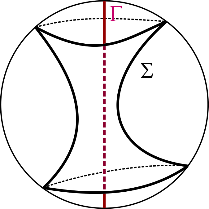
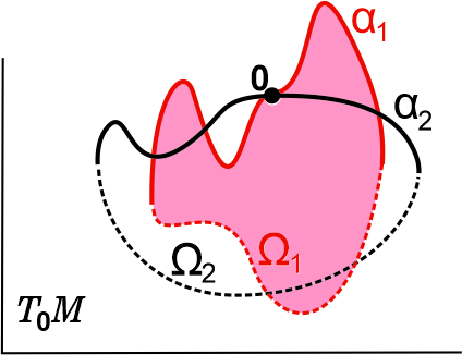
We say that a surface links a curve , if does not meet and it is homotopically non-trivial (relative to ) in (see Figure 1). An interesting consequence of Theorem B is the following corollary which is the analog of a result in due to Solomon [44].
Corollary.
Every embedded compact free boundary minimal surface of either meets or links each straight line passing through the origin.
In the proof of both Theorem A and Theorem B, we need the existence and regularity of a minimizer for a partially free boundary problem. Namely, let be a compact domain such that , where is a compact surface (not necessarily connected) with boundary, is a smooth, compact mean convex surface with boundary, which intersects ortogonally along , and (here denotes the topological interior of ). Let be a compact curve which is contained in and such that is either empty or consists of a finite number of points (the corners); and consider the class of surfaces in whose boundary minus is contained in . We look for a surface which has least area among all such surfaces. The existence of such surface follows from general compactness results about currents, and the regularity of away from the corners can be proved using results of [24, 26, 11] (see Section 3.2, Theorem 4). It was reported in [25] that for a problem similar to this one, the regularity at the corners would be settled in a work of Grüter and Simon (unpublished). In Section 3 we give the details of this proof in the case where intersects orthogonally by following the ideas contained in [25]. In particular, we prove the following regularity result.
Theorem C.
Suppose intersects orthogonally and is except possibly at a finite number of points. Then the minimizer for the partially free boundary problem described above is a connected oriented embedded minimal surface which meets orthogonally and is , in a neighborhood of each corner and is away from the corners and the possible isolated singularities of
The study of free boundary minimal surfaces (in euclidean domains) has attracted significant attention for several decades (see for instance classical works as [7, 27] or more recent results as [1, 2, 3, 6, 8, 20, 31, 32, 34, 35, 36, 38, 40, 43, 46, 50] and references therein). Recently there was an increase in interest for free boundary minimal surfaces in the unit euclidean 3-ball due to the work by Fraser and Schoen [16] (see also [17, 18]) where they made a connection between these objects and the Steklov eigenvalue problem. In analogy to Yau’s conjecture mentioned above, Fraser and Li [15] conjectured that the first nonzero Steklov eigenvalue of an embedded compact free boundary minimal surface in is equal to 1. This conjecture together with the Courant nodal domain theorem for the Steklov problem (stated for instance in [22], Section 6) implies the two-piece property for free boundary minimal surfaces in (see Remark 2). Hence, our result in Theorem A can be seen as an evidence to the conjecture by Fraser and Li.
In the last few years there have been many important studies about free boundary minimal surfaces. Ambrozio, Carlotto and Sharp [2] established compactness theorems for free boundary minimal hypersurfaces. Maximo, Nunes and Smith [35] proved the existence of free boundary minimal annuli through a degree argument. Li and Zhou [32] developed a min-max theory for free boundary minimal hypersurfaces.
We should mention that the class of free boundary minimal surfaces in is very rich. In fact, many techniques have been developed to construct new examples of free boundary minimal surfaces in . For instance, Fraser and Schoen [16, 18] constructed examples with genus and any number of boundary components. Using gluing methods, Folha, Pacard and Zolotareva [14] constructed examples with genus and any large number of boundary components, and also obtained examples of genus and large number of boundary components displaying similar asymptotic behavior to Fraser-Schoen family. Examples with large genus and boundary components were constructed by Ketover [30], where he also obtained examples with the symmetry group of the Platonic solids, both using min-max methods. Kapouleas and Li [28] also produced examples with large genus and boundary components, and examples with dihedral symmetry. Using gluing methods, Kapouleas and Wiygul [29] constructed examples with one boundary component and large genus, converging to an equatorial disk with multiplicity 3, as the genus goes to infinity. More recently, Carlotto, Franz and Schulz [5] applied min-max methods to prove the existence of embedded free boundary minimal surfaces with connected boundary and arbitrary genus.
This paper is organized as follows. In the second section we will prove both Theorem A and Theorem B; in Section 3 we will present the proof of the regularity at the corners of a minimizer for the partially free boundary problem mentioned above; and in Appendix A we will show an application of Serrin’s Maximum Principle (Lemma 2, [41]) at a corner.
Acknowledgements: The first author would like to thank Princeton University for the hospitality where part of the research and preparation of this article were conducted. The authors would like to thank the anonymous referee for valuable suggestions.
2. The two-piece property and other results
Throughout the paper we say that a curve in is a diameter if it is a straight line segment joining two antipodal points of and we will define an equatorial disk as the intersection of with a plane passing through the origin.
Given a surface in , we will write its boundary as where and
Definition 1.
Let be a compact surface properly immersed in We say that is a minimal surface with free boundary if the mean curvature vector of vanishes and meets orthogonally along (in particular, We say that is a minimal surface with partially free boundary if the mean curvature vector of vanishes and its boundary satisfies that meets orthogonally along and .
From now on, given a (partially) free boundary minimal surface with boundary , we will call its fixed boundary and its free boundary.
Lemma 1.
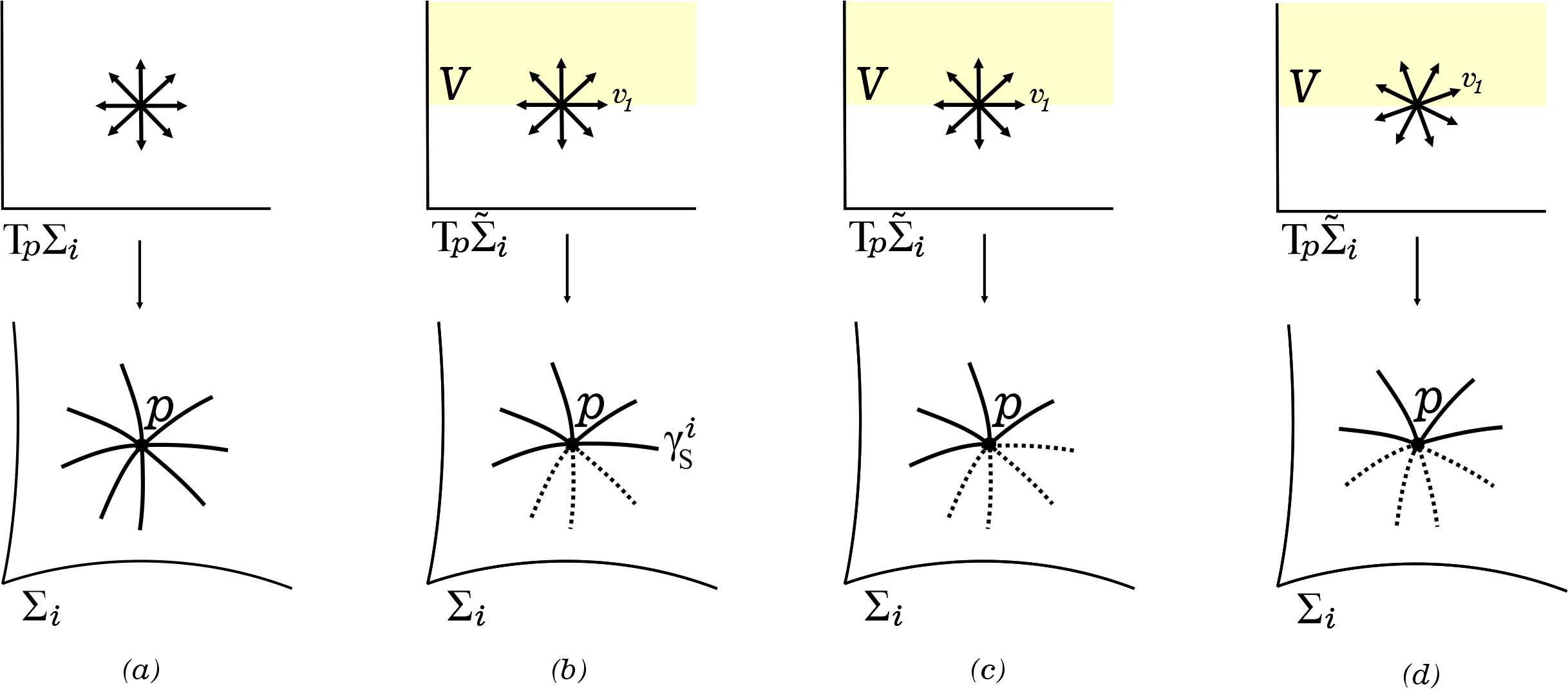
Let and be two distinct (partially) free boundary minimal surfaces with boundary that are tangent at a point Then
-
(1)
if , there exists a neighborhood of where the intersection is given by curves, , starting at and making equal angle. See Figure 2(a);
- (2)
In both cases, is called an -prong singularity.
Proof.
See [19, Lemma 1.4] for the proof of . For , it is known that any free boundary minimal surface can be extended analytically as a minimal surface in a neighborhood of each point of its free boundary (see Theorems 2 and 2’ in [9], pg. 178). So we can extend and on a neighborhood of . Denote by , , the extended surface from . In particular, and are two minimal surfaces tangent at an interior point. Then, by item , is given locally by curves, , starting at and making equal angle. Denote these curves by and by their tangent vectors at time zero. Denote by the (constant) angle between these vectors, and observe that and . Let be the half tangent plane of at the boundary point , that is, is the set of vectors such that there exists a curve with To simplify our notation, let us assume, without loss of generality, that is the half plane , , the sphere is centered at (0,1,0), and (after possibly reordering the vectors) is the vector with least angle from the positive -axis (counterclockwise). In particular, .
First observe that if then the vector is strictly pointing inside the sphere and, consequently, the arc is (locally) contained in
Suppose . Notice that since are real analytic, locally the intersection is either only the point or they coincide. If locally, then, by analyticity, locally the arc is necessarily either contained outside the sphere or inside the sphere; that is, the arc is either contained in or in . If locally, then the arc has to coincide with them. Let us remark that the same conclusions hold if , for some
Since we have at least four arcs and , there is at least one vector with Therefore, the intersection is given by curves, , starting at . ∎
Definition 2.
Let be a partially free boundary minimal surface in with piecewise smooth boundary . We say that is stable if for any function such that we have
| (2.1) |
or equivalently
| (2.2) |
where is the outward normal vector field to .
Lemma 2.
Let be a compact orientable immersed partially free boundary stable minimal surface in with piecewise smooth boundary . Suppose is contained in an equatorial disk. Then is totally geodesic. The same result holds in the case where has finite area and isolated singularities on .
Proof.
Let be as in the hypotheses and denote by the equatorial disk that contains its fixed boundary .
Let us first assume that the fixed boundary of does not have singularities.
Let be a vector orthogonal to the disk and consider the function , By hypothesis we know that , so (2.1) holds. Moreover, since is minimal, it is well-known that
| (2.3) |
On the other hand,
| (2.4) |
since is free boundary on .
If then is totally geodesic and we are done.
If for some then we can find a neighborhood of in such that is strictly positive. By (2.5), this implies for any , that is, is contained in the disk . Therefore, is entirely contained in the disk in particular, it is totally geodesic.
Now let us suppose that has isolated singularities in the fixed boundary (which is contained in the equatorial disk). Let us consider a cut-off function so that
-
•
for ,
-
•
for ,
-
•
, for some constant
and define as where In particular, we have
Now let us take the function . It satisfies and so (2.2) holds.
Observe that
and
since , and
Hence, applying it to (2.2), we get
| (2.6) |
Since has finite area and , we have
| (2.7) |
Therefore, we get the same conclusions as above. ∎
Remark 1.
Observe that by its proof, in order to be able to apply Lemma 2, we just need regularity and stability of the surface outside the equatorial disk where the fixed boundary is contained.
Remark 2.
Let be an embedded free boundary minimal surface in Recall that a nodal domain of a function is a maximally connected subset of the domain where the function does not change sign, and the Courant nodal domain theorem for the Steklov problem says that an eigenfunction corresponding to the -th nonzero Steklov eigenvalue has at most nodal domains. Let be a plane passing through the origin and let be a vector orthogonal to . The Jacobi function , defined in the proof of Lemma 2, is an eigenfunction with eigenvalue 1 for the Steklov problem. Hence, assuming Fraser-Li conjecture, it follows that has at most two nodal domains. Moreover, we can use the (interior and boundary) maximum principle with equatorial disks to conclude that has in fact two nodal domains, that is, the plane divides in excatly two connected surfaces. Hence, our result in Theorem 2 can be seen as an evidence to the conjecture by Fraser and Li.
Definition 3.
Let be a region in and let be a diameter. We say that is nullhomologous in if there exists a compact surface such that , where (see Figure 3).

The boundary of the region can be written as , where and In the next theorem we will denote by the closure of the component that is,
Theorem 1.
Let be a connected closed region with (non-strictly) mean convex boundary such that meets orthogonally along its boundary and is smooth. If contains a diameter , and is nullhomologous in , then is a closed halfball.
Proof.
Up to a rotation of around the origin, we can assume that is nonempty. Since is nullhomologous in , there is at least one curve such that there exists a surface contained in with boundary . We consider the class of admissible currents
where is the current associated to , and we minimize area (mass) in Then, by the results presented in Section 3, we get a compact embedded (orientable) partially free boundary minimal surface which minimizes area among compact surfaces in with boundary on the class in particular, its fixed boundary is exactly Moreover, by Proposition 2 in Section 3, either or
Claim 1.
is stable.
In the case , the surface is automatically stable in the sense of Definition 2, since it minimizes area for all local deformations. Suppose . For any with , consider defined by
and let be a first eigenfunction, i.e., .
Observe that although differently from the classical stability quotient (we have an extra term that depends on the boundary of ) we can still guarantee the existence of a first eigenfunction. In fact, since for any there exists such that , for any , we can use this inequality to prove that the infimum is finite. Once this is established the classical arguments to show the existence of a first eigenfunction work.
Since a.e., we have , that is, is also a first eigenfunction. Since , the maximum principle implies that in , in particular, does not change sign in . Then we can assume that in and, by continuity, we get in Therefore, we can use as a test function to our variational problem: Let be a smooth vector field such that for all , for all , and points towards along . Let be the flow of . For small enough the surfaces ; , are contained in . Since has least area among the surfaces , we know that
which implies that . Since is a first eigenfunction, we get that for any with . Therefore, we have stability for .
Then, since is contained in an equatorial disk, Lemma 2 implies that is necessarily a half disk. If , then we already conclude that has to be a halfball.
Suppose . Rotate around until the last time it remains in (this last time exists once is non empty), and let us still denote this rotated surface by . In particular, there exists a point where and are tangent. We will conclude that is necessarily a halfball.
In fact, if we can write locally as a graph over around and apply the classical Hopf Lemma; if we can use the Serrin’s Maximum Principle at a corner (see Appendix A for the details); and if we can apply (the interior or the free boundary version of) the maximum principle. In any case, we get that is a halfball.
∎
An equatorial disk divides the ball into two (open) halfballs. We will denote these two halfballs by and and we have
In the next proposition we will summarize some simple facts about partially free boundary minimal surfaces in which we will use in the proof of Theorem 2.
Proposition 1.
-
(i)
Let be an equatorial disk and let be a partially free boundary minimal surface in contained in one of the closed halfballs determined by and such that (if ). If is not an equatorial disk, then has necessarily nonempty fixed boundary and nonempty free boundary.
-
(ii)
The only (partially) free boundary minimal surface that contains an arc segment of a great circle in its free boundary is (contained in) an equatorial disk.
Proof.
If the free boundary were empty, we could apply the (interior) maximum principle with the family of planes parallel to the disk and conclude that should be a disk. On the other hand, if the fixed boundary were empty, then we would have a minimal surface entirely contained in a halfball without fixed boundary; hence, we could apply the (interior or free boundary version of) maximum principle with the family of equatorial disks that are rotations of around a diameter and conclude that should be a disk as well.
Let be an equatorial disk and suppose that is a (partially) free boundary minimal surface such that contains an arc segment in in particular, since they are both free boundary, we know they are tangent along Hence, given a point there exists a neighborhood of in where either is on one side of or is given by a collection of curves, , starting at (see Lemma 1). In this last case, for any point in , we will have a neighborhood where is on one side of ; therefore, in either case, applying the boundary maximum principle we can conclude that should be (contained in) an equatorial disk. ∎
Remark 3.
If and are two partially free boundary minimal surfaces in that intersect at a point transversally, then the intersection is locally given by a simple curve that meets orthogonally at . In fact, in the same way as we argued in the proof of Lemma 1, item , we can show that the intersection is locally given by a simple curve that meets at . Let be the normal vector to , Since they meet transversally, we know and, since is orthogonal to both . Therefore, meets orthogonally at .
Now we can prove the two-piece property for free boundary minimal surfaces in .
Theorem 2.
Let be a compact embedded free boundary minimal surface in Then for any equatorial disk , and are connected.
Proof.
If is an equatorial disk, then the result is trivial. So let us assume this is not the case.
Suppose that, for some equatorial disk , is a disjoint union of two nonempty open surfaces and , being connected. Notice that by Proposition 1(i) both and (all components of) have non empty fixed boundary and non empty free boundary.
Let us denote by the boundary of which is not necessarily connected. We can write , where is its fixed boundary () and is its free boundary (. Since and are two distinct minimal surfaces, either and are transverse or the intersection contains at least one -prong singularity (see Lemma 1).
Observe that, by applying (either the interior or free boundary version) of the maximum principle, we know that does not contain any isolated point in and, by Proposition 1(ii), does not contain any arc segment in .
Denote by and the closures of the two components of They are compact domains with mean convex boundary, and observe that the curve is the boundary of an orientable surface contained in them (in fact, is orientable and ). Hence, we can minimize area for the following partially free boundary problem (see Section 3.2):
We consider the class of admissible currents
where is the current associated to , and we minimize area (mass) in Then, by the results presented in Section 3, we get a compact embedded (orientable) partially free boundary minimal surface with fixed boundary and with possible isolated singularities in (see Theorem 4 and Remark 4). Moreover, by Proposition 2 in Section 3, either or
Arguing as in Claim 1 of Theorem 1, we can prove the stability of away from the disk . Since in the proof of Lemma 2, for the case where has isolated singularities, we only use stability away from the disk, we can still get the conclusion from Lemma 2, that is, each component of is a piece of an equatorial disk. The case can not happen because this would imply that is a disk, and we are assuming it is not. Therefore, only the second case can happen, that is, any component of meets only at points of Observe that each component of that is not bounded by a diameter is necessarily contained in . If some component of were bounded by a diameter, then we could apply Theorem 1 and would conclude that is an equatorial disk, which is not the case. Then is entirely contained in and, since , and does not contain any segment on , we have
Doing the same procedure as in the last paragraph for , we can construct another compact surface of with fixed boundary and such that and . Notice that is a surface without fixed boundary of , therefore In particular, which implies that has no fixed boundary, a contradiction (by Proposition 1(i)). Therefore, the theorem is proved. ∎
Corollary 3.
Every embedded compact free boundary minimal surface of either meets or links each diameter.
Proof.
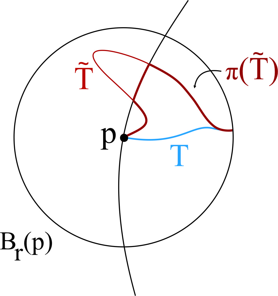
Let be a diameter with endpoints , and suppose does not meet . Write , where contains , and the decomposition is disjoint. Suppose, by contradiction, that is homotopically trivial (relative to ) in . We will prove that is nullhomologous in .
In fact, since is homotopically trivial in , we have that is a finite collection of simple closed curves in which are homotopically trivial in . Hence, there is a curve joining and ; and bounds a (topological) disk in . If , we are done. If that is not the case, by deforming , if necessary, we can suppose that and are transverse. Let be the unit normal vector field to pointing into , and denote by the intersection of with the boundary of a one-sided tubular neighborhood of (in the direction of ) of radius . We can choose small enough such that , and is transverse to . The intersection consists of a finite number of simple closed curves which bound open discs in (since is a disk). The set is a topological surface with and . Therefore is nullhomologous in .
Then, by Theorem 1, we conclude that is a closed halfball; in particular, is an equatorial disk. However, this contradicts the fact that . Therefore, links necessarily. ∎
3. Solution to a partially free boundary problem
3.1. Terminology
Let be an open set. We define
with the usual topology of uniform convergence of all derivatives on compact subsets. Its dual space is denoted by and the elements of are called -currents in . If , and is open, the mass of in is defined by
The boundary of is the -current given by
where denotes the exterior derivative operator.
Given a sequence in , we say that converges to as , if
Let denote the -dimensional Hausdorff measure. A set is called countably -rectifiable if is -measurable and if
where and for , is an -dimensional -submanifold of . Such possesses -a.e. an approximate tangent space .
A current is called integer multiplicity rectifiable, if
where is countably -rectifiable, is a locally -integrable integer valued function and, for -a.e. , , where is an orthonormal basis of the approximate tangent space . In this case, we write . Also, we denote by the Radon measure induced by the current .
An -varifold in is a Radon measure on , where is the Grassmannian of -hyperplanes in . An integer multiplicity rectifiable -varifold is defined by
where is countably -rectifiable and is a locally -integrable integer valued function. In particular, given an integer multiplicity rectifiable current, forgetting the orientation we have an associated integer multiplicity rectifiable varifold. Also, for we can define the first variation (see [42][chapter 4]), and for any -vector field , it holds the first variation formula
| (3.1) |
3.2. Minimizing Currents with Partially Free Boundary
Consider a compact domain such that , where is a compact surface (not necessarily connected) with boundary, is a smooth, compact mean convex surface with boundary, which intersects ortogonally along , and (here denotes the topological interior of ). Let be a compact -curve which is contained in and such that is either empty or consists of a finite number of points. We shall call the fixed boundary and the points of by corners.
Define the class of admissible currents by
where is the current associated to . We want to minimize area in , that is, we are looking for such that
| (3.2) |
The existence of the fixed boundary ensures that . It follows from [12, ], that the variational problem (3.2) has a solution (see also [23]). If is a solution we have
| (3.3) | |||||
| (3.4) | |||||
| (3.5) |
for any integer multiplicity current with compact support such that and .
In order to apply the known regularity theory for we need the following results.
Proposition 2.
If is a solution of (3.2), then either or .
Proof.
The proof follows the same ideas as in [47, Lemma A.1], so we only describe the construction needed and refer the reader to [47] for the details. Denote and let be the varifold associated to . Let be a vector field with compact support on such that for any , and on , where is the inward pointing unit normal of . By (3.3) we have
| (3.6) |
Suppose that does not contain . By the main result in [45], does not intersect the interior of (the result in [45] is stated in the case where is a minimal surface and is stationary but, as remarked at the end of the paper, the proof also works in our more general situation).
Suppose there is a point . Let be a diffeomorphism which is associated with an extension of . By [47, Lemma A.2], there exist and a neighborhood of such that, for any and any non negative function with , there exist functions , , satisfying the following:
-
(1)
the graphs of foliate ,
-
(2)
meets orthogonally along , ,
-
(3)
, has mean curvature equal to (with respect to the downward pointing normal vector of the graph),
-
(4)
for any .
In [47], is a minimal surface; however, the construction relies on the implicit function theorem and uses [48, Appendix] and [2, Section 3], with a small modification on the map needed, thus it also works if is mean-convex.
Moreover, we can choose small enough such that and choose so that if for , then . Let be the smallest so that intersects . Then necessarily, which implies that does not intersect ; hence, the intersection occurs at the interior or at the free boundary of . However, observe that by construction has mean curvature vector pointing towards so, by the main results of [49] and [33], the graph of can not intersect neither at the interior nor at the free boundary, which is a contradiction. Although in [33] the varifold is assumed to be stationary, the proof is by contradiction and relies on the construction of a vector field as above such that ; hence, it also works on our case. ∎
Proposition 3.
Let . If is a solution of (3.2), then there exists a uniform constant such that for sufficiently small we have
for any such that and is compact, and .
Proof.
To simplify the notation let us write to denote
Denote by the nearest point projection onto . Observe that in a piece of a tubular neighborhood of containing the map is well defined, piecewise smooth and Lipschitz. Consider such that is well defined in . Observe that we can find a constant (independent of ) such that
Let be as in the statement of the proposition. Denote (see Figure 4). Then,
| (3.7) |
for some constant . So the proof is complete. ∎
We then have the following regularity result.
Theorem 4.
Let be a solution of (3.2). Then, away from the corners, is supported in a connected oriented embedded minimal -surface, which meets orthogonally along .
Proof.
From the classical interior regularity theory developed by DeGiorgi (here ), see [12], we know that in a neighborhood of each , T is given by (-times, ) integration over an embedded minimal surface. The regularity near a point at the fixed part of the boundary away from the corners follows from the work of Hardt and Simon [26] on the case , and for the case we can use, by Proposition 3 and Remarks 0.2 and 0.3 in [11], the results in [11] (let us remark that in the proof of Theorem 6 we will get to this same situation after a reflection and we will give more details on how to use the results in [11]). Since by Proposition 2 the free part of the boundary is contained in , we can use the result by Grüter [24] to conclude the regularity at the free boundary (away from the corners). Therefore, away from the corners, is supported in a connected oriented embedded minimal -surface, which meets orthogonally along . ∎
It remains the question about the regularity of at the corners. In [25], Grüter reports joint work with L. Simon (unpublished) where they would prove regularity in a similar situation. We develop here the ideas present in [25] to prove the regularity for the case where meets orthogonally.
Arguing as in Section of [24], we can reduce the problem of local regularity at a corner to the following situation. Applying a translation and a dilation if necessary we can suppose one of the corners is located at the origin and the open ball (centered at the origin with radius 3) is decomposed by into two open -cells, that is
| (3.8) |
where and are homeomorphic to the -dimensional unit ball and the decomposition is disjoint.
Consider a rectifiable of integer multiplicity satisfying:
| (3.9) | |||
| (3.10) | |||
| (3.11) | |||
| (3.12) |
for every open set and for any integer multiplicity current such that and . It also holds , for every open set .
3.3. Regularity at the corner
Extend to a closed smooth surface such that a tubular neighborhood of contains (applying a dilation if necessary). Define the reflection across by
where is defined as the unique point in such that . Since our questions are local, we can ensure that is well defined (after a dilation if necessary) and continuously differentiable. Geometrically we can see as follows: the line through with direction (a unit normal vector to at ) is parametrized by , so if , we have . It is easy to see that .
Define . Thus has integer multiplicity, and
| (3.13) |
Moreover, . Denote and by . Hence, has integer multiplicity, finite mass and the support of its boundary is contained in .
Now we will prove that is regular at and, of course, this implies the regularity of at . For this purpose, we will first adapt some ideas of [24] to show that has a tangent cone at which is area-minimizing.
Lemma 3.
Consider , where and is a unit normal vector to at . Then, for small enough, the derivative of satisfies
| (3.14) |
where is a positive constant.
Proof.
Given and , consider a curve such that and . Then
So, , and by Taylor’s theorem we have for small enough
where , for some constant . By the computation above,
where is the supremum of the norm of the second fundamental form of . Therefore, the result follows. ∎
Lemma 4.
There exists .
Proof.
The surface separates the ball in two connected components and . Suppose (without loss of generality) . Let be an open set such that for some . Let be of integer multiplicity such that and . Denote by the nearest point projection onto . Arguing as in Proposition 3 we conclude that there is a constant such that
| (3.15) |
Now let be an open set such that and for some . Let be of integer multiplicity such that and . We can write
where , , since . By (3.15), for sufficiently small we have
Thus
| (3.16) |
For sufficiently small, denote by the closed ball centered at the origin with radius . Consider the curve and take the current where is the cone over , and is the strip bounded by and the two radii joining to the endpoints of (see Figure 5). Observe that for some constant and by the coarea formula
To simplify our notation, let us denote Observe that , so by , we have
for some constant . Hence,
| (3.17) |
Define . By the coarea formula
thus
| (3.18) |
Define where is a differentiable function which will be chosen later. We have for a.e.
Taking , we have and for a.e. In particular, the function is non-decreasing and, therefore, exists. ∎
Definition 4.
Consider the map defined by , . If , we simply write . Suppose is integer multiplicity and . If there exist a sequence converging to and an integer multiplicity current such that
we call an oriented tangent cone to at .
Theorem 5.
There is an oriented tangent cone to at such that is an oriented straight line. Moreover,
-
(1)
is minimizing in , that is, for any open set and any integer multiplicity current satisfying and , we have
-
(2)
if we have
Proof.
Consider a sequence converging to . By Lemma 4, we have
Since meets orthogonally at , we have that is a -curve. Indeed, it is clearly , and since is , its derivative is Lipschitz, so this also holds for the duplicate curve. Hence, there exists
therefore,
Thus, from the compactness theorem for integer multiplicity currents (see [12, 4.2.17]), a subsequence of converges to a current and the boundaries converge to (in the subsequence). Furthermore, since is a -curve, it has an oriented tangent line at . In particular, . At the end of this proof we will show that is a cone.
Let be an open set and fix so that . Let be integer multiplicity such that and . Choose a sequence with and Define . We have ; hence, for large enough, and . Then, it follows from (3.16) that
| (3.20) | |||||
where we used Lemma 4 in the last inequality.
Since , and because of the lower-semi-continuity of mass, a standard argument using (3.20) yields that
Next we will prove in the sense of Radon measures. Consider a compact set and an open set containing . For any , define such that in some neighborhood of and
Consider
hence, for , we have .
Using (3.20) and proceeding as in the proof of [42, Theorem 34.5], we conclude that , where . So,
Since (by construction) we obtain
Hence, letting , it follows that
| (3.21) |
By the lower semi-continuity of mass with respect to weak convergence, we have
| (3.22) |
Since (3.21) and (3.22) hold for arbitrary compact and open , it follows by a standard approximation argument that
| (3.23) |
Finally, choose such that (which is true except possibly for countably many ). Then, (3.23) implies that
Thus
| (3.24) |
Finally, since is area-minimizing, it is a stationary varifold. So, using (3.24) in the monotonicity identity at the boundary (see [4, equation 31]) for we have
| (3.25) |
where and is a conormal to . Since is a line containing , the second integral on (3.25) vanishes. So, we can argue as in [42, Theorem ] to conclude that is a cone. ∎
Theorem 6.
There is a neighborhood of such that is an embedded oriented -surface with boundary, for .
Proof.
Since meets orthogonally, the set is a -surface; hence, it satisfies an exterior ball condition at (there exists a ball which is tangent to at ). Also, . From Proposition and equation (3.16), there is a constant such that
| (3.26) |
for any , and any such that and .
Now we can argue as in [11, Lemma 1.1] (we will only sketch the arguments and refer the reader to [11] for the details). Denote . One can construct a (topological) surface with boundary, denoted by , which is contained in the closure of and such that . Observe that . Then, using the decomposition of codimension one currents [42, Theorem 27.6] and arguing as in [11], we find a family of open sets , where , , and such that for some we have
| (3.27) | |||
| (3.28) |
and and each satisfy an almost-minimizing property like (3.26).
Consider , , such that its support contains and denote by its tangent cone at . Also, denote by the tangent cone of at . The existence of the cones and the fact that each is area-minimizing follows as in Theorem 5. Also, there exist open sets , a half-space and a half-plane such that , , and for . Thus is a multiplicity one half-plane and each must be a multiplicity one plane for . In particular, and , for . Since is a -curve, we can use the results of [10] to conclude that and each are -surfaces, for , in some neighborhood of .
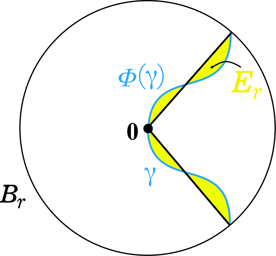
By Proposition 2, either or . In the first case we already have regularity, so suppose the second case happens. Our final step is to show that each is actually an empty set. Fix for . By (3.28), we know that is on one side of . Since is a multiplicity one plane, then it is necessarily the tangent plane to at (otherwise there would be points of in ). Hence, since and are tangent at , they can be written locally as graphs over closed regions and of their tangent plane (with possibly ); that is, there exists a closed neighborhood of in such that and , where and with . Observe that since is tangent to at and has no boundary, the point is not a corner for , just a point in its boundary.
Let and be two arcs of the curves and respectively, that contain the origin . We can see the arc as the graph over a curve in Furthermore, as everything is local, we can see as the graph of a function with Hence, we have and we can assume that (see Figure 6). Observe that since is tangent to at and transversal to , the curves and are tangent at in particular, we can assume that
Since is there exists a constant such that
which implies
Hence,
Taking , we get
Call . We have that is a function with and Therefore, we can find a domain containing the origin with boundary which contains the graph of (see Figure 7). In particular, has a Dini continuous normal and a Hopf-type lemma can be applied to (see, for instance, [39, Theorem 1.3], or the notes at pg. 46 of [21]). Since is mean convex, is minimal (by the regularity of the original current , Theorem 4) and is on one side of , we can apply the Hopf Lemma to and conclude that its normal derivative at the origin has a strict sign. However, this is not true once and are tangent at Thus is empty.

∎
Therefore, combining all the regularity results from Sections 3.2 and 3.3, we get the following theorem.
Theorem 7.
Let be a solution of (3.2), where is a curve. Then is supported in a connected oriented embedded minimal surface, which meets orthogonally along and it is , , in a neighborhood of and away from .
Remark 4.
If has isolated singularities (for example, -prong singularities) at the interior or the boundary, the same regularity result holds true for points away from these singularities.
Appendix A A maximum principle at a corner
Here we are going to show a kind of a maximum principle at a corner that we use in the proof of Theorem 1.
As in Section 2, given a region , we will denote by the closure of the part of the boundary of contained in int.
Theorem 8.
Let be a connected closed region with (non-strictly) mean convex boundary such that meets orthogonally along its boundary and is smooth. Suppose there is a closed half-disk contained in and denote by one of its corners. If is tangent to at then is necessarily a halfball.
Proof.
Let be the plane containing . We are assuming that and are tangent at Observe that, by the classical (interior or free boundary version of the) maximum principle, we already know that either is a halfball or is contained in the diameter of (see the proof of Theorem 1 for more details).
We can choose coordinates so that is tangent to the circumference at in and belongs to the halfplane containing , is in the direction of its diameter and coincides with the outward conormal vector to , and is the normal vector to pointing towards at the points .
Since is locally on one side of , if we define as we can take sufficiently small so that can be written as a graph over a region in containing . Consider the orthogonal projection onto We are choosing the unit normal vector to pointing into that is, . Denote by We have and we can write with and , since they are tangent at .
If is a parametrization of the boundary of , then parametrizes We have
in particular, and is tangent to . Thus, up to a change of orientation, and consequently, that is, is tangent to at the origin (which is identified with by our choice of coordinates).
Since is mean convex and is contained in its mean convex side, we know its mean curvature satisfies for the choice of normal . Moreover, satisfies the mean curvature equation
| (A.1) |
Observe that since is tangent to at the origin, we know contains a segment of the diameter starting at ; hence, choosing a smaller if necessary, we can assume that . Let us consider the region . Since is exactly the disk containing we know that Denote by the component of the boundary of contained in the -axis. By our choice of coordinates we know that on and, since we are assuming that is contained in the diameter of , we have on .
Hence, we can apply Serrin’s Maximum Principle (see Lemma 2 in [41]) to conclude that, since , either or , for every vector pointing strictly into . (Observe that the operator defined in (A.1) satisfies the hypotheses of [41, Lemma 2]).
If we conclude that is a halfball and then , which contradicts our assumption that is contained in the diameter of . Suppose the second option happens, that is,
| (A.2) |
for any vector with coordinates and Then, by continuity, we get that
Denote by the outward conormal vector to . Since meets orthogonally, coincides with the position vector along the boundary of Since for the -coordinate we know that restricting to we obtain
| (A.4) |
where in graph coordinates. Since is tangent to the -axis at we can write in a neighborhood of as a graph , for some function . In particular, and Hence, we can rewrite (A.4) as
Differentiating the previous equation with respect to we obtain
Thus, when we evaluate at , using (A.3) and the facts that and , we conclude that . However, this together with (A.3) implies that , which contradicts (A.2).
Therefore, we have which implies that is contained in the plane and, consequently, is necessarily a halfball. ∎
References
- [1] L. Ambrozio, A. Carlotto and B. Sharp, Index estimates for free boundary minimal hypersurfaces, Math. Ann. 370 (2018), 1063–1078.
- [2] L. Ambrozio, A. Carlotto and B. Sharp, Compactness analysis for free boundary minimal hypersurfaces, Calc. Var. Partial Differential Equations 57 (2018), no. 1, Art. 22, 39 pp.
- [3] L. Ambrozio and I. Nunes, A gap theorem for free boundary minimal surfaces in the three-ball, Preprint at arXiv:1608.05689, to appear at Comm. Anal. Geom. (2016).
- [4] T. Bourni, Allard-type boundary regularity for boundaries, Adv. Calc. Var. 9 (2016), no. 2, 143–161.
- [5] A. Carlotto, G. Franz and M. Schulz, Free boundary minimal surfaces with connected boundary and arbitrary genus, Preprint at arXiv:2001.04920 (2020).
- [6] J. Chen, A. Fraser and C. Pang, Minimal immersions of compact bordered Riemann surfaces with free boundary, Trans. Am. Math. Soc. 367 (2015), no. 4, 2487–2507.
- [7] R. Courant, The existence of minimal surfaces of given topological structure under prescribed boundary conditions, Acta Math. 72 (1940), 51–98.
- [8] B. Devyver, Index of the critical catenoid, Geom. Dedicata 199 (2018), 355–371.
- [9] U. Dierkes, S. Hildebrandt and A. Tromba, Regularity of minimal surfaces, Grundlehren der math. Wiss. 340, Springer, Heidelberg 2010.
- [10] F. Duzaar and K. Steffan, Optimal interior and boundary regularity for almost minimizers to elliptic variational integrals, J. Reine Angew. Math. 546 (2002), 73–138.
- [11] N. Edelen, A note on the singular set of area-minimizing hypersurfaces, Calc. Var. Partial Differential Equations 59 (2020), no. 1, Art. 18, 9 pp.
- [12] H. Federer, Geometric measure theory, Grundlehren der math. Wiss. 153. Springer, New York 1969.
- [13] H. Federer, The singular sets of area minimizing rectifiable currents with codimension one and of area minimizing flat chains modulo two with arbitrary codimension, Bull. Amer. Math. Soc. 76 (1970), 767–771.
- [14] A. Folha, F. Pacard and T. Zolotareva, Free boundary minimal surfaces in the unit 3-ball, Manuscripta Math. 154 (2017), no. 3-4, 359–409.
- [15] A. Fraser and M. Li, Compactness of the space of embedded minimal surfaces with free boundary in three-manifolds with nonnegative Ricci curvature and convex boundary, J. Differential Geom. 96 (2014), 183–200.
- [16] A. Fraser and R. Schoen, The first Steklov eigenvalue, conformal geometry, and minimal surfaces, Adv. Math. 226 (2011), no. 5, 4011–4030.
- [17] A. Fraser and R. Schoen, Minimal surfaces and eigenvalue problems, Contemp. Math. 599 (2013), 105–121.
- [18] A. Fraser and R. Schoen, Sharp eigenvalue bounds and minimal surfaces in the ball, Invent. Math. 203 (2016), no. 3, 823–890.
- [19] M. Freedman, J. Hass and P. Scott, Least area incompressible surfaces in -manifolds, Invent. Math. 71 (1983), 609–642.
- [20] B. Freidin, M. Gulian and P. McGrath, Free boundary minimal surfaces in the unit ball with low cohomgeneity, Proc. Am. Math. Soc. 145 (2017), no. 4, 1671–1683.
- [21] D. Gilbarg and N. S. Trudinger, Elliptic Partial Differential Equations of Second Order, Classics in Mathematics. Springer, Berlin (1998).
- [22] A. Girouard and I. Polterovich, Spectral geometry of the Steklov problem, Preprint at arXiv:1411.6567v1 (2014).
- [23] M. Grüter, Regularitt von minimierenden Strömen bei einer freien Randbedingung, Universitt Düsseldorf, 1985.
- [24] M. Grüter, Optimal regularity for codimension one minimal surfaces with a free boundary, Manuscripta Math. 58 (1987), no. 3, 295–343.
- [25] M. Grüter, A remark on minimal surfaces with corners, Variational methods (Paris, 1988), 273–282.
- [26] R. Hardt and L. Simon, Boundary regularity and embedded solutions for the oriented Plateau problem, Ann. of Math. (2) 110 (1979), no. 3, 439–486.
- [27] S. Hildebrandt, J. C. C. Nitsche, Minimal surfaces with free boundaries, Acta Math. 143 (1979), no. 3–4, 251–272.
- [28] N. Kapouleas and M. Li, Free boundary minimal surfaces in the unit three-ball via desingularization of the critical catenoid and the equatorial disk, Preprint at arXiv:1709.08556 (2017).
- [29] N. Kapouleas and D. Wiygul, Free-boundary minimal surfaces with connected boundary in the 3-ball by tripling the equatorial disc, Preprint at arXiv:1711.00818v2 (2017).
- [30] D. Ketover, Free boundary minimal surfaces of unbounded genus, Preprint at arXiv:1612.08692 (2016).
- [31] M. Li, A general existence theorem for embedded minimal surfaces with free boundary, Commun. Pure Appl. Math. 68 (2015), no. 2, 286–331.
- [32] M. Li and X. Zhou, Min-max theory for free boundary minimal hypersurfaces I-regularity theory, Preprint at arXiv:1611.02612 (2016).
- [33] M. Li and X. Zhou, A maximum principle for free boundary minimal varieties of arbitrary codimension, Preprint at arXiv:1708.05001 (2017).
- [34] V. Lima, Bounds for the Morse index of free boundary minimal surfaces, Preprint at arXiv:1710.10971 (2017).
- [35] D. Máximo, I. Nunes and G. Smith, Free boundary minimal annuli in convex three-manifolds, J. Differ. Geom. 106 (2017), no. 1, 139–186.
- [36] P. McGrath, A characterization of the critical catenoid, Indiana Univ. Math. J. 67 (2018), no. 2, 889–897.
- [37] A. Ros, A two-piece property for compact minimal surfaces in a three-sphere, Indiana Univ. Math. J. 44 (1995), no. 3, 841–849.
- [38] A. Ros, Stability of minimal and constant mean curvature surfaces with free boundary, Mat. Contemp. 35 (2008), 221–240.
- [39] M. Safonov, On the boundary estimates for second order elliptic equations, Complex Var. Elliptic Equ. 63 (2018), 1123–1141.
- [40] P. Sargent, Index bounds for free boundary minimal surfaces of convex bodies, Proc. Amer. Math. Soc. 145 (2017), no. 6, 2467–2480.
- [41] J. Serrin, A symmetry problem in potential theory, Arch. Rational Mech. Anal. 43 (1971), 304–318.
- [42] L. Simon, Lectures on geometric measure theory, Proceedings of the Centre for Mathematical Analysis, Australian National University, vol. 3, Australian National University, Centre for Mathematical Analysis, Canberra, 1983. vii+272 pp.
- [43] G. Smith and D. Zhou, The Morse index of the critical catenoid, Geom. Dedicata 201 (2018), 13–19.
- [44] B. Solomon, Harmonic maps to spheres, J. Differential Geom. 21 (1985), 151–162.
- [45] B. Solomon and B. White, A strong maximum principle for varifolds that are stationary with respect to even parametric elliptic functionals, Indiana Univ. Math. J. 38 (1989), no. 3, 683–691.
- [46] H. Tran, Index characterization for free boundary minimal surfaces, Preprint at arXiv: 1609.01651 (2016).
- [47] Z. Wang, Existence of infinitely many free boundary minimal hypersurfaces, Preprint at arXiv:2001.04674 (2020).
- [48] B. White, Curvature estimates and compactness theorems in 3-manifolds for surfaces that are stationary for parametric elliptic functionals, Invent. Math. 88 (1987), no. 2, 243-256.
- [49] B. White, The maximum principle for minimal varieties of arbitrary codimension, Comm. Anal. Geom. 18 (2010), no. 3, 421–432.
- [50] R. Ye, On the existence of area-minimizing surfaces with free boundary, Math. Z. 206 (1991), no. 3, 321–331.