-operator bounds on angle-integrated absorption and thermal radiation for arbitrary objects
Abstract
We derive fundamental per-channel bounds on angle-integrated absorption and thermal radiation for arbitrary bodies—for any given material susceptibility and bounding region—that simultaneously encode both the per-volume limit on polarization set by passivity and geometric constraints on radiative efficiencies set by finite object sizes through the scattering -operator. We then analyze these bounds in two practical settings, comparing against prior limits as well as near optimal structures discovered through topology optimization. Principally, we show that the bounds properly capture the physically observed transition from the volume scaling of absorptivity seen in deeply subwavelength objects (nanoparticle radius or thin film thickness) to the area scaling of absorptivity seen in ray optics (blackbody limits).
Motivated by the increasing control of light offered by micro and nanoscale structuring Koenderink et al. (2015); Molesky et al. (2018), impetus to find bounds analogous to the blackbody limit for geometries that violate the assumptions of ray optics (nanoparticles Du and Yu (2017), thin films Tong et al. (2015), photonic crystals Zhu et al. (2015); Ilic et al. (2016), etc.) has steadily grown over the past few decades. It is now well established that the absorption (radiative thermal emission) cross-sections of a compact object can be much greater than its geometric area Bohren and Huffman (2008); Tribelsky (2011); Ruan and Fan (2011); Biehs and Ben-Abdallah (2016); Fernández-Hurtado et al. (2018); Thompson et al. (2018) (“super-Planckian” emission), and that deeply subwavelength films can achieve near unity absorptivity via surface texturing Kats and Capasso (2016); Dyachenko et al. (2016). Limits applicable to all length scales and materials could both provide insight into these representative phenomena and guide efforts in related application areas such as integrated and meta-optics Kruk and Kivshar (2017); Khorasaninejad and Capasso (2017); Hampson et al. (2018), photovoltaics Yablonovitch (1982); Atwater and Polman (2010); Zhang et al. (2016); Jariwala et al. (2017), and photon sources Thompson et al. (2013); Galfsky et al. (2015); Somaschi et al. (2016).
Development of bounds for arbitrary objects have primarily followed two overarching strategies: modal decompositions based on quasi-normal, singular value, Fourier and/or multipole expansions McLean (1996); Hamam et al. (2007); Kwon and Pozar (2009); Yu et al. (2010a, b); Ruan and Fan (2010); Hugonin et al. (2015); Jia et al. (2015); Yang et al. (2017), relating absorption cross-section to the number of excitable optical modes (channels); or material/region bounds, utilizing energy Callahan et al. (2012); Miller et al. (2016) and/or spectral sum rules Fuchs and Liu (1976); Miller (2000, 2007); Miller et al. (2014); Shim et al. (2019) to constrain achievable properties. Separately, each of these approaches present challenges for photonic design. Modal decompositions incorporate the specific size and shape characteristics of a body through expansion coefficients, and hence, inherently, require some enumeration and characterization of the participating modes to determine the range of values these coefficients can take Hamam et al. (2007); Ruan and Fan (2012); Alpeggiani et al. (2017). Although fundamental considerations (transparency, energy, size, etc.) can and have been used in this regard Miller (2000); Sohl et al. (2007); Yu et al. (2010a); Yang et al. (2017), such cut-offs have yet to tightly bound potential coefficient values for arbitrary compact geometries, particularly when applied to metallic nanoparticles and antennas Gustafsson et al. (2007); Kwon and Pozar (2009); Miller et al. (2016). Conversely, material bounds set by intrinsic dissipation naturally reproduce the volumetric scaling of absorptivity characteristic of deeply subwavelength objects (and are highly accurate for the special case of weak polarizability in this regime Miller et al. (2016)). However, because such approaches intrinsically suppose an optimally large response field existing at all points within an arbitrary object for any incident field, the same volumetric scaling persists for all length scales. Consequently, material bounds can rapidly become too loose beyond quasi-static settings, yielding unphysical divergences with both increasing object size and material response.
In this letter, we derive bounds on thermal radiation and absorption that combine these two approaches, linking the impact of material response with the influence of an object’s geometry through the scattering -operator.
This leads to a per-channel limit on integrated absorption capturing both extraction and radiative (scattering) loss processes through the singular values of the imaginary part of the vacuum Green function.
The result is applicable to objects of any size, exhibiting a smooth transition in absorptivity from the volume scaling achievable in the quasi-static (deeply-subwavelength) regime to the area scaling limit of macroscopic ray optics.
Further, the bounds always asymptotically approach the ray optics limit (when all characteristic lengths are large) and diverge sub-logarithmically (rather than linearly) with material quality for objects of finite extent, significantly reducing cross-section limits for typical optical media even when all characteristic lengths are small.
Throughout, we compare the present results to prior bounds as well as structures discovered using topology optimization, realizing a variety of examples (metallic and dielectric) that nearly achieve the predicted limits.
Derivation—From the relations of scattering theory, both the power scattered from an incident field (), and the thermal radiation emitted at temperature , can be expressed in terms of the scattering -operator of an object and the vacuum Green function Krüger et al. (2012) as
| (1) |
and,
| (2) |
Here, is the angular frequency, is the wavenumber, is the impedance of free-space, with is the Planck energy of a harmonic oscillator, denotes the trace, , and, by Kirchhoff’s law of thermal radiation, is the object’s angle integrated absorption Greffet and Nieto-Vesperinas (1998). (A synopsis of scattering formalism, along with a derivation of (2), is provided in Supplemental Material Molesky et al. (2019a).) For a passive object, scattered power must be positive for any incident field. As such, (1) simultaneously dictates that all singular values of the -operator must be smaller than the material figure of merit
| (3) |
which was similarly derived in Ref. Miller et al. (2016) for polarization fields, and that is positive-definite.
As is real-symmetric positive-definite, it can be expressed via a singular value decomposition as
| (4) |
where, as supported by our later analysis, each (eigenvalue) can be equated to the outgoing radiative flux of the th mode—the th radiative efficacy of the domain. (The set plays an analogous role to the coupling coefficients used by D.A.B. Miller in setting limits on far-field optical communication Miller (2000).) Consider (2) using this expansion, Now, take to be a general operator described by the properties (reciprocity), (passivity), and positive-definite (passivity), ignoring all other physical constraints that any true -operator must satisfy. In this context, two characteristics of any maxima of are clear. First, as the appearance of any cross-terms () will always decrease . Therefore, to maximize , a general operator must be diagonalized in the basis of , (4). Second, the complex phase of only influences the first (positive) piece of the sum, and so the value of peaks when Together, these two considerations show that achievable values of are bounded by taking to be diagonalized by (4) with purely imaginary eigenvalues: with . As such,
| (5) |
and maximizing the contribution of each yields
| (6) |
That is, based on the criterion , each channel in (6) produces either the Landauer limited contribution of Molesky et al. (2019b), or the material limited .
Interpretation—In terms of the operator, the total power extracted from any incident field by an object is .
Comparing with (1) and (2), thus amounts to the difference of the extracted () and scattered () power for free-space states.
The separation of these two forms persists throughout the derivation of the bounds, representing the linear and quadratic terms of (5).
results from their connected physics.
In real space, is the integral of the local density of free-space states over the domain of the object. Following (6), the total power that can be extracted by an object, the first term of (2), is thus bounded by its ability to interact with radiative modes, , which is maximized (independently) under complete saturation of material response, . Relatedly, this form is also the result of applying the per-volume (shape independent) optical response limit of Ref. Miller et al. (2016) to integrated absorption, and is similar to the light trapping bound of Ref. Callahan et al. (2012). Due to these connections with prior work,
| (7) |
serves as a useful comparison for , and is subsequently referred to as the quasi-static bound. This name is chosen as (7) follows from the assumption that the interaction of the object with any incident field is identically material limited, which can occur in quasi-static settings. This does not mean that is valid only under the quasi-static approximation. Like , is a mathematical bound derived from Maxwell’s equations, albeit for any selection of parameters
In (5) and (6) this extracted power contribution is suppressed by scattering (radiative) losses, which are captured in the quadratic term in (2) as the coupling of the polarization currents generated within an object back to free-space modes: originating through the operator , each represents the ability of the object to convert a given field into a current, and each radiative efficacy the conversion of a current into outgoing radiative flux. Equivalently, the presence of strong polarization currents, necessary for strong per-volume absorption, leads to radiative loses, and these loses limit possible absorption.
If , mirroring the observed dependencies of absorption () and scattering () seen in highly subwavelength metallic antennas Hamam et al. (2007); Ruan and Fan (2010), the growth of radiative losses with increasing can potentially
surpass the growth of the extracted power, inducing saturation.
As both processes are rooted in the same conversion between radiative fields and polarization currents, this critical coupling occurs at the compelling value of Pendry (1983, 1999), the probability of a maximally entropic Bernoulli process, resulting in the Landauer limit value of .
Analysis—The practical usefulness of (6) stems from its favorable mathematical properties.
Namely, (6) monotonically increases with or any , and, as proved in Supplementary Material Molesky et al. (2019a), each increases if the object grows (domain monotonicity).
This allows us to freely decouple any true object from an imagined encompassing region of space (bounding domain).
A mismatch between the domain of the object and the domain of must technically reduce below , but without any modification (6) remains an upper bound on .
That is, the result of (6) for any particular bounding domain is applicable to any object that can be enclosed (as well as any sub-domain).
The procedure for calculating is straightforward for any bounding geometry (e.g. wires, disks, spheres, extended films, stars, disconnected patches, etc.). Precisely, the set of singular values of the domain can always be computed by forming a real space matrix representation of ,
| (8) |
with every multiplied by a hidden , and then performing a singular value decomposition of the result Polimeridis et al. (2013, 2015). Here, to facilitate further investigation, we will focus on the high symmetry case of a ball where semi-analytic evaluation is manageable (expressions for films, as well as minor additional details, are given in Supplemental Material Molesky et al. (2019a)). Nevertheless, we stress that determining for domains lacking symmetry does not raise any meaningful computationally difficulties.
For this geometry two types of singular values arise
| (9) |
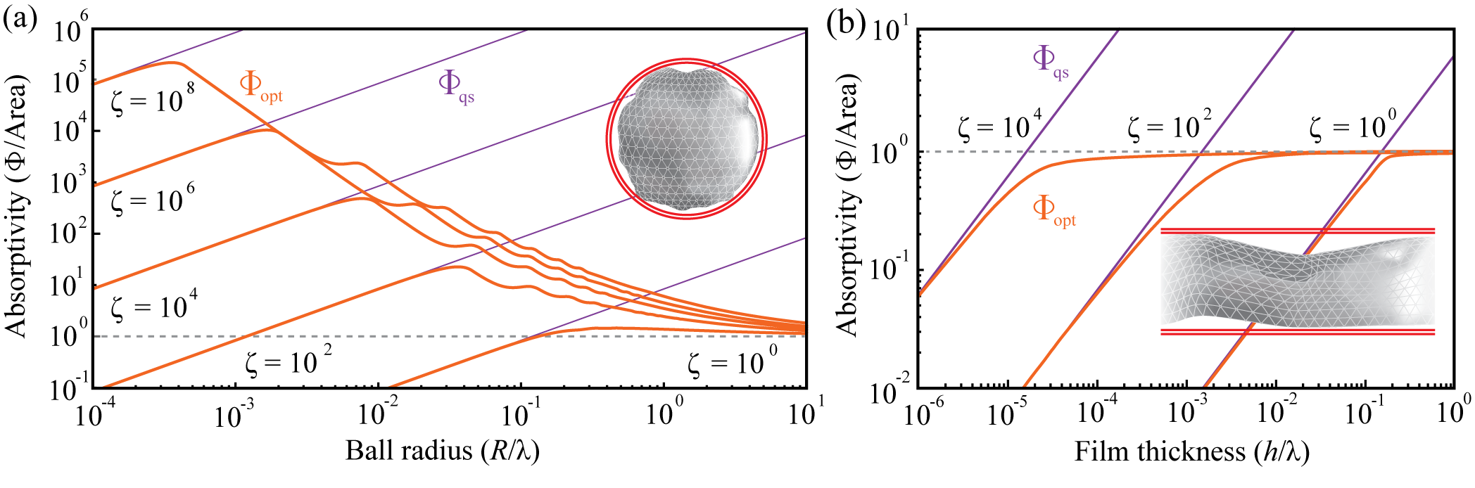
where is the th Bessel function of the first kind with an additional factor of included in its argument, each (spherical harmonic) index has a multiplicity of , and is the radius of the ball normalized by the wavelength. Using standard properties of Bessel functions, it can be shown that for values of , each of these singular values tends to the asymptote , and that for any combination of arguments and (asymptotically approached for small values of ). These forms reveal two prescient general features. First, in the limit of small domains (), with “small” being determined by the value of , only the first singular value of the first type contributes, and this triply degenerate (dipole) mode is responsible for the initial volume scaling necessitated by the physical meaning of the bounds. Second, the radial growth of the singular values shows that the saturation condition (impact of radiative losses) plays a major role in limiting radiative thermal emission and integrated-absorption in wavelength scale volumes. (For , Fig. 1 (a), radiative losses lead to order of magnitude deviations of from beyond .) As visually confirmed by Fig. 1 panel (a), as the domain grows an increasing number of channels (multipoles) saturate causing “steps” to appear in , and these steps lead to successively larger deviation with that ultimately regularize the initial volumetric scaling. Results for films, Fig. 1 (b), are qualitatively similar. However, since the domain is infinite, the steps associated with saturation are now blended into a continuum, and the large characteristic size limit is approached from below rather than above. From a practical perspective, the fact that can achieve near ideal absorptivity for very small film thickness and moderate values of is quite remarkable, a finding that is tacitly supported by a number of recent studies in 2D materials and meta-surfaces Thongrattanasiri et al. (2012); Akselrod et al. (2015); Kim et al. (2018); Nong et al. (2018). Crucially, in either case, for any value of , asymptotes to a geometric perfect absorber (the blackbody limit).
The asymptotic behavior of the singular values also reveals general characteristics of the dependence of on the material figure of merit . Applying Sterling’s approximation to the bounding expressions given above, for we have and , to arbitrary accuracy as becomes large. Fix , and suppose that ( is analogous). Using the fact that the remaining (unsaturated) linear contribution of is then bounded by . Hence, as saturates increasingly higher spherical harmonics, the contribution of the remaining unsaturated harmonics becomes increasingly small compared to the contribution of the newly saturated harmonic, . But, saturation of the th singular value (in the large limit) requires
| (10) |
which has a sub-logarithmic dependence between and . Due to domain monotonicity, the above material scaling result for a ball is applicable to all compact (finite sized) objects.
This bound on material quality scaling is well matched to the features of the curves in Fig. 1 panel (a). Once the radius has surpassed , geometric increases in () produce relatively minute changes in the bounds. This behavior also appears for smaller radii at larger values of , but this range is not of great practical relevance since materials with surpassing are quite rare. For instance, in the optical to infrared, , has a peak value of approximately for gold, for tungsten, for silicon carbide, for silicon, for gallium arsenide, and for gallium phosphide Palik (1998).
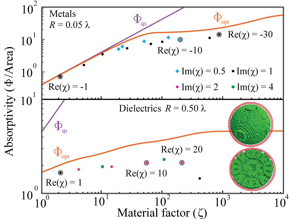
Optimizations—Case evidence for the tightness of (6) is presented in Fig. 2. Using a gradient topology optimization algorithm Jensen and Sigmund (2011); Molesky et al. (2018), see Supplemental Material for details Molesky et al. (2019a), structures nearly achieving have been discovered for two widely different domain sizes ( and ) and a variety of metallic and dielectric susceptibilities. In Fig. 2, these media are grouped by imaginary susceptibility, corresponding to four different values of , , with the remaining variation in occurring due to . Explicit values of are given for circled points, providing a sense of the range considered. As was previously remarked by O. Miller et al. Miller et al. (2016), is attained for a plane wave polarized along the axis of an ellipsoidal metallic nanoparticle, given a properly chosen aspect ratio. For small values of this ratio is near unity and resonant metallic structures () matching both bounds are easily discovered. As moves to moderate values, the aspect ratio required for an ellipsoidal particle to match becomes increasingly extreme. Due to our chosen spherical boundary, discovered structures begin to deviate considerably from , but continue to come within a factor of of up to . Past this point, numerical issues impede our present algorithms and it remains to be seen how much of the roughly order of magnitude headroom allowed by is accessible.
Results for the larger domain, Fig. 2 (b), show similarly good agreement.
An example structure is depicted in the right inset (full view and planar cut), corresponding to the rightmost green square in the plot.
Comparing with the assumptions made in deriving (6), the operator
for this structure (, ) is indeed found to be nearly diagonal in the basis of and have almost completely imaginary eigenvalues (for supporting data see Supplemental Material Molesky et al. (2019a)).
Remarks—There are a few points that should be considered when using (6), or comparing to prior literature.
First, is a bound on thermal emission and integrated absorption for a given domain and factor.
By choosing different geometries and material parameters, (6) can be applied to any desired context, but the confining volume is an essential feature.
Second, there is no universal guarantee of tightness.
Beyond the demonstrated agreement of the bounds with known quasi-static and ray optics asymptotics, the only a priori guarantee is domain monotonicity; there are likely volumes and material parameters where the value of will be larger than the true of any practical structure.
Next, while we have only considered single wavelengths, there is no reason the bounds can not be applied to finite frequency ranges.
The derivation of presented above does not incorporate any spectral sum rules (derived from causality), such as the fact that should obey Kramers-Kronig dispersion relations, but for resonant absorption or thermal emission simply multiplying the bound by the width of the resonance should not produce a substantially looser bound than at the peak wavelength.
(As an expedient, taking to be the peak value of a Lorentzian function of width is likely a fair approximation.)
Finally, as suggested in the introduction, can be interpreted as the extension of prior multipole analysis McLean (1996); Hamam et al. (2007); Kwon and Pozar (2009); Yu et al. (2010a, b); Ruan and Fan (2010); Hugonin et al. (2015); Jia et al. (2015); Yang et al. (2017), or communication limits Miller (2000, 2007), to general domains with the crucial addition that an upper bound is set on the number modes which may contribute through the pseudo-rank of the imaginary part of the vacuum Green function () and the material figure of merit () (3).
We foresee this rank revealing capability potentially providing a number of benefits for future practical design and optimization.
We also note that much of what has been developed in this manuscript is applicable not only to generalized electromagnetic scattering (for incident planewaves or dipolar emitters with applications to solar cells, light-emitting diodes, and single-photon emitters), but also to quantum mechanics, acoustics, and other wave physics.
I Acknowledgments
This work was supported by the National Science Foundation under Grants No. DMR-1454836, DMR 1420541, DGE 1148900, the Cornell Center for Materials Research MRSEC (award no. DMR1719875), the Defense Advanced Research Projects Agency (DARPA) under agreement HR00111820046, and the National Science and Engineering Research Council of Canada under PDF-502958-2017. The views, opinions and/or findings expressed herein are those of the authors and should not be interpreted as representing the official views or policies of any institution. We thank Jason Necaise for performing instructive calculations of the bounds in cylindrical coordinates.
II Supplementary Information
-operator definition—Following the Lippmann-Schwinger approach to scattering Lippmann and Schwinger (1950), the -operator is formally defined through the self-consistent equation
| (11) |
as
| (12) |
with the “inc” subscript denoting an initial (freely incident)
current (field), the vacuum Green function,
and a generalized electromagnetic susceptibility. A lack
of any subscript indicates total field quantities.
Heat transfer to thermal emission—In two recent (related) articles Jin et al. (2019); Molesky et al. (2019b) we have established that the heat transfer between any two bodies, labeled and , can be written in terms of the scattering -operator as
| (13) |
where and are mutual scattering operators defined as
| (14) |
To produce an expression for thermal emission, we will evaluate (13) in the limit that one of the objects, here chosen to be , tends to a blackbody. Abstractly, a blackbody is an encompassing, infinitely large, region capable of perfectly absorbing any incident field: physically, a spherical material shell of inner radius and outer radius , in the simultaneous limit and with and . We begin by breaking (13) into
| (15) |
where is the current dressing operator (producing a total current from an initial current). As tends to the blackbody limit, the above definition shows that , i.e. that the total electric current density tends to the free current density. Hence, tends to zero, and the mutual scattering operators and become and respectively. Therefore,
| (16) |
with and the volume of becoming arbitrarily large.
Now, for any collection of objects, the fluctuation dissipation theorem Eckhardt (1984) states that
| (17) |
which in our notation becomes
| (18) |
To apply this result to (13), we imagine a fictitious addition to body that perfectly overlaps with . Since and body has a finite extent, this addition will have no material effect on the value produced by (13). However, its inclusion shows that consistent application of the blackbody limit must result in
| (19) |
Applying this result to (13), using the simplification of (16), we find that
| (20) |
where in the middle expression has been used for the blackbody limit inside body .
Domain monotonicity– Let be a subdomain of , and
| (21) |
be the vacuum Green functions for each of these volumes. Assume that these sums are finite. The first singular vector, corresponding to the largest singular value, is equivalent to the complex vector field maximizing the integral
| (22) |
subject to the constraint,
. It is clear that moving to a larger volume is always favourable in
this context. In the worst case
simply does not change. Therefore, the largest singular value of
is domain monotonic. Now, suppose
that all singular values up to have been shown to be domain
monotonic, so that , and
consider . Recall that the singular vector
is defined by the property of maximizing
subject to the constraints and . Take
to be the projection of onto the subdomain . If spans
, then we essentially return to
the case of the first singular vector. is
orthogonal to all , and
zero outside . Hence, it is orthogonal to all
. As ,
with the added freedom of the additional volume we must have
. If does not span
, then some elements of
are orthogonal to
all . Select one such vector and
denote it as . Since , by the preceding argument .
Singular values for balls—To derive the singular values of
for a ball we have followed the formulation in
Tsang et al. Tsang et al. (2004). In this work, it is shown
that
| (23) |
where
| (24) |
and is the th spherical with additional factor of included in its argument. In these definition, are the vector spherical harmonics, obeying the orthogonality conditions
| (25) |
(As the spherical harmonics are unaffected by projection into a connected volume, the program given below is also valid for shells and other homeomorphic domains.) Comparing (23) with a standard singular value decomposition, we equate the value of the inner product of the vector pairs forming the above outer products with the singular values of . Performing the angular integrals over the vector spherical harmonics, results in two types of singular values quoted in the main text
| (26) |
Singular values for films—Calculation of the singular values for films of thickness follows a similar procedure to that of a ball. Using results from Tsang et al. Tsang et al. (2004) and Krüger et al. Krüger et al. (2012), the imaginary part of the Green function can generally be decomposed in terms of “regularized” spectral basis as . The “propagating” basis functions of this set are orthogonal to one other (though not necessarily self-normalizable), and form a complete set both at the origin and at infinity. In particular, considering the in-plane wavevector , the basis functions can be written as plane waves , with denoting the parity and the polarization. The vacuum Green function in this basis then takes on the form
| (27) |
with singular vector functions given by
| (28) |
in position space, where is real and nonnegative by virtue of the restriction to propagating waves. The inner products may then all be written as
| (29) |
due to the orthogonality of these basis functions. This immediately yields the desired singular values corresponding to each :
| (30) |
Inverse design—To explore the largest possible design space, the optimizations shown in the text result from the “topology” (density) approach Molesky et al. (2018), in which each pixel (permittivity value) within the chosen bounding domain is considered as an independent design parameter. The key to the tractability of such large-scale optimizations is the use of gradient-based optimization algorithms (the method of moving asymptotes is employed in our algorithm Svanberg (2002)). To make use of these approaches, each pixel is initially treated as continuous. That is, at each position in the domain, we begin by assign a parameter and state that the susceptibility of that pixel is
| (31) |
where is the material susceptibility. An initial optimization is then carried out using NLOPT Johnson (2014), producing a “gray” structure in which many take on intermediate () values. In subsequent optimizations (for the same structure) these values are then binarized (i.e. forcing or ) by enclosing in function, , which is slowly changed from the linear relation given above to a smooth approximation of the step function Jensen and Sigmund (2011).
The primary challenge of this type of inverse design approach for the problem we have considered lies in the cost of computing for inhomogeneous medium, which typically needs to be evaluated thousands of times in a single optimization iteration. To surmount this difficulty, we have exploited our previously discussed fluctuating volume current formulation Polimeridis et al. (2015); Jin et al. (2016). This framework allows for two major simplifications. First, it removes the necessity of simulating space outside the bounding domain, as would be necessary to accurately calculate emitted thermal radiation or angle-integrated absorption using a finite difference approach. Second, it allows the central matrix-vector multiplication that is used by the iterative inversion solver Polimeridis et al. (2015), in (33), to be computed via fast-Fourier transforms. To further reduce computational cost, we also use the fact that has low pseudo-rank. (In a similar spirit to the derivation of the optimal -operator given the main text, we use foreknowledge of the number of modes that will possibly contribute to select an appropriate algorithm and pre-allocate computational resources.) This allows us to formulate the scattering inversion problem, (33), directly in terms of a singular value decomposition (SVD) of , which can be approximated to any accuracy with efficient randomized methods Hochman et al. (2014). (For a full discussion of this procedure see Refs. Halko et al. (2011); Martinsson et al. (2011); Polimeridis et al. (2015).) Specifically, starting from an equivalent trace form of heat transfer to the one given in the main text, the singular value decomposition of allows us to recast as
| (32) |
where the subscript denotes the Frobenius norm. Evaluation of (32) requires only one inverse solve for each column of the low rank decomposition:
| (33) |
(32) is also well suited to calculation of the gradient of . Starting from this result, using (31), direct application of matrix calculus shows that
| (34) |
and the total gradient is then
| (35) |
As before, only a number solves equal to the rank of the singular value decomposition of the imaginary part of the Green function are required to evaluate (35) for all design parameters.
Singular values of from inverse design—As a
point of comparison with the assumptions made in deriving
, we have explored the
-operator for the dielectric structure of the rightmost
green square in Fig. 2 (, ) in the
basis of . This physical realization
proves to nearly satisfy both the assumption of asymmetry
() and simultaneous diagonalizability. Specifically, we find that
The ratio of the true values of in comparison to the ideal values determined by are given in Tab.1 below. These values are naturally grouped by a singular value type index () and the spherical harmonic index. For clarity, an average is taken over the (ideally constant) harmonic subindex. The final column gives the weight that each entry makes to .
| -Type | Ideal Value | Average Ratio | Weight |
References
- Koenderink et al. (2015) A. F. Koenderink, A. Alu, and A. Polman, Science 348, 516 (2015).
- Molesky et al. (2018) S. Molesky, Z. Lin, A. Y. Piggott, W. Jin, J. Vucković, and A. W. Rodriguez, Nature Photonics 12, 659 (2018).
- Du and Yu (2017) P. Du and J. S. Yu, Chemical Engineering Journal 327, 109 (2017).
- Tong et al. (2015) J. K. Tong, W.-C. Hsu, Y. Huang, S. V. Boriskina, and G. Chen, Scientific Reports 5, 10661 (2015).
- Zhu et al. (2015) L. Zhu, A. P. Raman, and S. Fan, Proceedings of the National Academy of Sciences 112, 12282 (2015).
- Ilic et al. (2016) O. Ilic, P. Bermel, G. Chen, J. D. Joannopoulos, I. Celanovic, and M. Soljačić, Nature Nanotechnology 11, 320 (2016).
- Bohren and Huffman (2008) C. F. Bohren and D. R. Huffman, Absorption and scattering of light by small particles (John Wiley & Sons, 2008).
- Tribelsky (2011) M. I. Tribelsky, Europhysics Letters 94, 14004 (2011).
- Ruan and Fan (2011) Z. Ruan and S. Fan, Applied Physics Letters 98, 043101 (2011).
- Biehs and Ben-Abdallah (2016) S.-A. Biehs and P. Ben-Abdallah, Physical Review B 93, 165405 (2016).
- Fernández-Hurtado et al. (2018) V. Fernández-Hurtado, A. I. Fernández-Domínguez, J. Feist, F. J. García-Vidal, and J. C. Cuevas, Physical Review B 97, 045408 (2018).
- Thompson et al. (2018) D. Thompson, L. Zhu, R. Mittapally, S. Sadat, Z. Xing, P. McArdle, M. M. Qazilbash, P. Reddy, and E. Meyhofer, Nature 561, 216 (2018).
- Kats and Capasso (2016) M. A. Kats and F. Capasso, Laser & Photonics Reviews 10, 735 (2016).
- Dyachenko et al. (2016) P. N. Dyachenko, S. Molesky, A. Y. Petrov, M. Störmer, T. Krekeler, S. Lang, M. Ritter, Z. Jacob, and M. Eich, Nature Communications 7, 11809 (2016).
- Kruk and Kivshar (2017) S. Kruk and Y. Kivshar, ACS Photonics 4, 2638 (2017).
- Khorasaninejad and Capasso (2017) M. Khorasaninejad and F. Capasso, Science 358, eaam8100 (2017).
- Hampson et al. (2018) S. Hampson, W. Rowe, S. D. Christie, and M. Platt, Sensors and Actuators B: Chemical 256, 1030 (2018).
- Yablonovitch (1982) E. Yablonovitch, JOSA 72, 899 (1982).
- Atwater and Polman (2010) H. A. Atwater and A. Polman, Nature Materials 9, 205 (2010).
- Zhang et al. (2016) N. Zhang, C. Han, Y.-J. Xu, J. J. Foley IV, D. Zhang, J. Codrington, S. K. Gray, and Y. Sun, Nature Photonics 10, 473 (2016).
- Jariwala et al. (2017) D. Jariwala, A. R. Davoyan, J. Wong, and H. A. Atwater, ACS Photonics 4, 2962 (2017).
- Thompson et al. (2013) J. D. Thompson, T. Tiecke, N. P. de Leon, J. Feist, A. Akimov, M. Gullans, A. S. Zibrov, V. Vuletić, and M. D. Lukin, Science 340, 1202 (2013).
- Galfsky et al. (2015) T. Galfsky, H. Krishnamoorthy, W. Newman, E. Narimanov, Z. Jacob, and V. Menon, Optica 2, 62 (2015).
- Somaschi et al. (2016) N. Somaschi, V. Giesz, L. De Santis, J. Loredo, M. P. Almeida, G. Hornecker, S. L. Portalupi, T. Grange, C. Antón, J. Demory, C. Gómez, I. Sagnes, N. D. Lanzillotti-Kimura, A. Lemaítre, A. Auffeves, A. G. White, L. Lanco, and P. Senellart, Nature Photonics 10, 340 (2016).
- McLean (1996) J. S. McLean, IEEE Transactions on Antennas and Propagation 44, 672 (1996).
- Hamam et al. (2007) R. E. Hamam, A. Karalis, J. D. Joannopoulos, and M. Soljačić, Physical Review A 75, 053801 (2007).
- Kwon and Pozar (2009) D.-H. Kwon and D. M. Pozar, IEEE Transactions on Antennas and Propagation 57, 3720 (2009).
- Yu et al. (2010a) Z. Yu, A. Raman, and S. Fan, Proceedings of the National Academy of Sciences 107, 17491 (2010a).
- Yu et al. (2010b) Z. Yu, A. Raman, and S. Fan, Optics Express 18, A366 (2010b).
- Ruan and Fan (2010) Z. Ruan and S. Fan, Physical Review Letters 105, 013901 (2010).
- Hugonin et al. (2015) J.-P. Hugonin, M. Besbes, and P. Ben-Abdallah, Physical Review B 91, 180202(R) (2015).
- Jia et al. (2015) Y. Jia, M. Qiu, H. Wu, Y. Cui, S. Fan, and Z. Ruan, Nano Letters 15, 5513 (2015).
- Yang et al. (2017) Y. Yang, O. D. Miller, T. Christensen, J. D. Joannopoulos, and M. Soljacic, Nano Letters 17, 3238 (2017).
- Callahan et al. (2012) D. M. Callahan, J. N. Munday, and H. A. Atwater, Nano letters 12, 214 (2012).
- Miller et al. (2016) O. D. Miller, A. G. Polimeridis, M. T. H. Reid, C. W. Hsu, B. G. DeLacy, J. D. Joannopoulos, M. Soljačić, and S. G. Johnson, Optics Express 24, 3329 (2016).
- Fuchs and Liu (1976) R. Fuchs and S. Liu, Physical Review B 14, 5521 (1976).
- Miller (2000) D. A. B. Miller, Applied Optics 39, 1681 (2000).
- Miller (2007) D. A. B. Miller, JOSA B 24, A1 (2007).
- Miller et al. (2014) O. D. Miller, C. W. Hsu, M. T. H. Reid, W. Qiu, B. G. DeLacy, J. D. Joannopoulos, M. Soljačić, and S. G. Johnson, Physical review letters 112, 123903 (2014).
- Shim et al. (2019) H. Shim, L. Fan, S. G. Johnson, and O. D. Miller, Physical Review X 9, 011043 (2019).
- Ruan and Fan (2012) Z. Ruan and S. Fan, Physical Review A 85, 043828 (2012).
- Alpeggiani et al. (2017) F. Alpeggiani, N. Parappurath, E. Verhagen, and L. Kuipers, Physical Review X 7, 021035 (2017).
- Sohl et al. (2007) C. Sohl, M. Gustafsson, and G. Kristensson, Journal of Physics D: Applied Physics 40, 7146 (2007).
- Gustafsson et al. (2007) M. Gustafsson, C. Sohl, and G. Kristensson, Proceedings of the Royal Society A: Mathematical, Physical and Engineering Sciences 463, 2589 (2007).
- Krüger et al. (2012) M. Krüger, G. Bimonte, T. Emig, and M. Kardar, Physical Review B 86, 115423 (2012).
- Greffet and Nieto-Vesperinas (1998) J.-J. Greffet and M. Nieto-Vesperinas, JOSA A 15, 2735 (1998).
- Molesky et al. (2019a) S. Molesky, W. Jin, P. S. Venkataram, and A. W. Rodriguez, Supplemental material including references Lippmann and Schwinger (1950); Jin et al. (2019); Molesky et al. (2019b); Eckhardt (1984); Tsang et al. (2004); Krüger et al. (2012); Molesky et al. (2018); Svanberg (2002); Johnson (2014); Jensen and Sigmund (2011); Polimeridis et al. (2015); Jin et al. (2016); Hochman et al. (2014); Halko et al. (2011); Martinsson et al. (2011). (APS, 2019).
- Molesky et al. (2019b) S. Molesky, P. S. Venkataram, W. Jin, and A. W. Rodriguez, arXiv preprint arXiv:1907.03000 , 12 (2019b).
- Pendry (1983) J. Pendry, Journal of Physics A: Mathematical and General 16, 2161 (1983).
- Pendry (1999) J. Pendry, Journal of Physics: Condensed Matter 11, 6621 (1999).
- Polimeridis et al. (2013) A. G. Polimeridis, F. Vipiana, J. R. Mosig, and D. R. Wilton, IEEE Transactions on Antennas and Propagation 61, 3112 (2013).
- Polimeridis et al. (2015) A. G. Polimeridis, M. T. H. Reid, W. Jin, S. G. Johnson, J. K. White, and A. W. Rodriguez, Physical Review B 92, 134202 (2015).
- Thongrattanasiri et al. (2012) S. Thongrattanasiri, F. H. Koppens, and F. J. G. De Abajo, Physical Review Letters 108, 047401 (2012).
- Akselrod et al. (2015) G. M. Akselrod, J. Huang, T. B. Hoang, P. T. Bowen, L. Su, D. R. Smith, and M. H. Mikkelsen, Advanced Materials 27, 8028 (2015).
- Kim et al. (2018) S. Kim, M. S. Jang, V. W. Brar, K. W. Mauser, L. Kim, and H. A. Atwater, Nano letters 18, 971 (2018).
- Nong et al. (2018) J. Nong, H. Da, Q. Fang, Y. Yu, and X. Yan, Journal of Physics D: Applied Physics 51, 375105 (2018).
- Palik (1998) E. D. Palik, Handbook of optical constants of solids, Vol. 3 (Academic Press, 1998).
- Jensen and Sigmund (2011) J. S. Jensen and O. Sigmund, Laser & Photonics Reviews 5, 308 (2011).
- Lippmann and Schwinger (1950) B. A. Lippmann and J. Schwinger, Physical Review 79, 469 (1950).
- Jin et al. (2019) W. Jin, S. Molesky, Z. Lin, and A. W. Rodriguez, Phys. Rev. B 99, 041403 (2019).
- Eckhardt (1984) W. Eckhardt, Physica A: Statistical Mechanics and its Applications 128, 467 (1984).
- Tsang et al. (2004) L. Tsang, J. A. Kong, and K.-H. Ding, Scattering of electromagnetic waves: theories and applications, Vol. 27 (John Wiley & Sons, 2004).
- Svanberg (2002) K. Svanberg, SIAM Journal on Optimization 12, 555 (2002).
- Johnson (2014) S. G. Johnson, URL ab-initio.mit.edu/nlopt (2014).
- Jin et al. (2016) W. Jin, A. G. Polimeridis, and A. W. Rodriguez, Physical Review B 93, 121403 (2016).
- Hochman et al. (2014) A. Hochman, J. Fernandez Villena, A. G. Polimeridis, L. M. Silveira, J. K. White, and L. Daniel, IEEE Transactions on Antennas and Propagation 62, 3150 (2014).
- Halko et al. (2011) N. Halko, P.-G. Martinsson, and J. A. Tropp, SIAM review 53, 217 (2011).
- Martinsson et al. (2011) P.-G. Martinsson, V. Rokhlin, and M. Tygert, Applied and Computational Harmonic Analysis 30, 47 (2011).