Realistic sensitivity curves for pulsar timing arrays

Abstract

We construct realistic sensitivity curves for pulsar timing array searches for gravitational waves, incorporating both red and white noise contributions to individual pulsar noise spectra, as well as the effect of fitting to a pulsar timing model. We demonstrate the method on both simulated pulsars and a realistic array consisting of a subset of NANOGrav pulsars used in recent analyses. A comparison between the results presented here and exact sensitivity curves shows agreement to tens of percent. The resulting sensitivity curves can be used to assess the detectability of predicted gravitational-wave signals in the nanohertz frequency band in a fraction of the time that it would take to compute the exact sensitivity curves.

I Motivation

Pulsar timing arrays (PTAs) are poised to make the first detection of nanohertz gravitational waves (GWs) in the next 2-5 years Siemens et al. (2013); Rosado et al. (2015); Taylor et al. (2016); Kelley et al. (2017). These galactic-scale GW detectors use the correlated times of arrival (TOAs) from millisecond pulsars to search for GWs Sazhin (1978); Detweiler (1979); Foster and Backer (1990). The recent inception of observational relativity by the advanced LIGO and VIRGO ground-based detectors Abbott et al. (2016, 2018) and the multi-messenger observations of binary neutron stars Abbott et al. (2017) have drastically changed our understanding of stellar-mass compact objects. PTAs are poised to complement these observations by observing GWs from binary systems comprised of super-massive black holes (SMBHs) in the centers of distant galaxies.

A common tool used to assess the observability of GW sources across the spectrum are detection sensitivity curves (see, e.g., Moore et al. (2015a); Robson et al. (2019) and Figure 1). These curves are basic “figures of merit,” constructed by the developers of GW observatories to assess the sensitivity of current detectors and to predict the sensitivity of future, next-generation detectors. The wider astrophysics community uses detection sensitivity curves as an initial estimate of the ability of a given detector to observe GWs from a particular source.

While detailed sensitivity curves for extant detectors are usually published for each observation run, those for PTAs are often simplified Hobbs (2011); Thrane and Romano (2013), only including identical white-noise components and often assuming that all pulsar observation epochs are evenly spaced and have the same baseline of observations. When drawn, these curves are often cut-off at the timespan of the observations and do not include important insensitivities at frequencies of $1/{\rm yr}$ and $2/{\rm yr}$, due to fitting for a pulsar’s astrometric parameters (Figure 1).

Figure 1: Sensitivity curves for different GW observations and the predicted spectra of various GW sources. Note, in particular, the (over) simplicity of the PTA sensitivity curves relative to those for LISA and LIGO. The goal of our paper is to construct more realistic PTA sensitivity curves. (Figure taken from Hobbs (2011).)

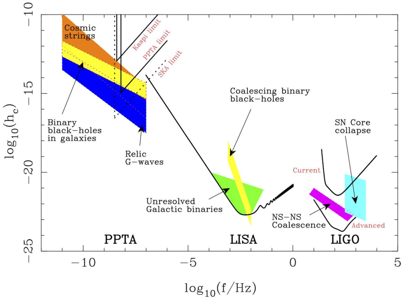
It has long been known that the fit to a pulsar’s timing model acts as a filter function Cordes (1980); Blandford et al. (1984), absorbing frequencies in the pulsar timing data in a predictable manner. These effects have been studied in the context of searches for GWs Cutler et al. (2014); Taylor et al. (2016); Blandford et al. (1984). Reference Madison et al. (2013) go one step further, showing how one can mitigate for losses in sensitivity using very-long-baseline interferometry to localize pulsars sky locations without explicitly fitting for their positions using the timing data.

Modern PTA data analysis strategies and algorithms are designed with this complication of the timing model fit in mind Demorest (2007); van Haasteren et al. (2009); Coles et al. (2011); van Haasteren and Levin (2013); Chamberlin et al. (2015); Lee et al. (2012); Lee (2016). This formalism was used e.g., in Moore et al. (2015b) to study PTA sensitivity curves for deterministic and stochastic sources of GWs, calculating sensitivity curves both analytically and numerically, using frequentist and Bayesian methods. The approach in Moore et al. (2015b) is similar in spirit to ours in that they start from the same likelihood function as we do (Section II.2), and they use properties of the expected signal-to-noise ratios for deterministic and stochastic GW signals to start to incorporate the effect of timing model fits. Our analysis differs from theirs in that we explicitly identify a component of the likelihood function that encodes both the noise power spectral density in a given pulsar’s data set and the effects of the timing model fit. This information is combined with known sources of realistic noise in pulsar timing data, including time-correlated (red) noise, to construct sensitivity curves for individual pulsars. (Reference Caballero et al. (2016) also discusses the effect of red noise on the sensitivity of pulsar timing searches for GWs, using a Fisher matrix calculation to estimate the errors.) For an array of pulsars, we use the expected signal-to-noise ratio of detection statistics for both deterministic and stochastic GW signals to construct effective sensitivity curves for the whole array.

I.1 Plan of paper

In Section II, we describe the basic formalism underlying pulsar timing analyses—i.e., timing residuals, timing models, and the effect of fitting to a timing model. This leads us to timing-model-marginalized residuals and their associated transmission functions, which play a key role in the subsequent construction of detection sensitivity curves. In Section III, we describe in detail the response of pulsar timing measurements to both deterministic and stochastic GWs. Then, in Section IV, we introduce detection statistics for both types of signals. The expressions for their corresponding expected signal-to-noise ratios allow us to read off an effective strain-noise power spectral density for the PTA, which has the interpretation of a detection sensitivity curve. As an application of our analysis, we construct sensitivity curves for the NANOGrav 11-yr pulsars using realistic noise properties and timing model fits, and compare our predicted sensitivities to published upper limits. We conclude in Section V. We also include Appendix A, in which we cast the results of an early seminal paper Blandford et al. (1984) into the more modern notation used in recent pulsar timing analyses.

The calculations provided in this work are packaged in a Python package available on the Python Package Inventory (PyPI) and GitHub.

II Pulsar timing analyses

Here we review the formalism underlying pulsar timing analyses used in GW searches. Readers interested in more details should see Blandford et al. (1984); Demorest (2007); Ellis et al. (2012); van Haasteren and Levin (2013); Chamberlin et al. (2015).

II.1 Times of arrival and timing residuals

Let us start with a single pulsar. The measured pulse times of arrival (TOAs) consist of three parts:

$$t=t^{\rm det}(\xi)+n+h\,.$$ (1)

The first term gives the expected TOAs due to deterministic processes, which depend on intrinsic properties of the pulsar (e.g., its spin period, period derivative, …), extrinsic properties of the pulsar (e.g., its sky location, proper motion, distance from the solar system barycenter, …), and processes affecting the pulse propagation (e.g., disperion delays due to the interstellar medium, relativistic corrections, …). The timing model parameters are denoted by $\xi$. The second term is (stochastic) noise intrinsic to the pulsar or to the measurement process itself. The third term is a perturbation to the pulse arrival times induced by GWs, which in general will have contributions from both deterministic and stochastic sources, $h=h^{\rm det}+h^{\rm stoch}$.

Timing residuals are then defined by subtracting the expected TOAs (predicted by the timing model for an initial estimate of the model parameters $\xi_{0}$) from the measured TOAs:

$$\delta t\equiv t-t^{\rm det}(\xi_{0})=M\,\delta\xi+n+h\,,$$ (2)

where

$$M\equiv\left(\frac{\partial t^{\rm det}}{\partial\xi}\right)\bigg{|}_{\xi=\xi_{0}}$$ (3)

is the design matrix. The above expression for $\delta t$ is obtained by Taylor expanding the timing model $t^{\rm det}(\xi)$ around the initial parameter estimates $\xi_{0}$, assuming that the initial estimates are close enough to the true values that only 1st-order terms in the parameter deviations $\delta\xi$ are needed in the expansion. The design matrix $M$ is a rectangular matrix of dimension $N\times N_{\rm par}$, with components $M_{ia}$. Each column of the design matrix encodes the linearized fit to one parameter in the timing model.

II.2 Fitting to a timing model

From the form of (2), one sees that errors $\delta\xi$ in our orignal estimate $\xi_{0}$ of the timing model parameters lead to deterministic features in the timing residuals. For example, an error in the pulse period leads to timing residuals that grow linearly with time, $\delta t\sim t$, while an error in the period derivative leads to residuals that grow quadratically with time, $\delta t\sim t^{2}$. Thus, we can improve our estimates of the timing model parameters by fitting for $\delta\xi$ in our linear timing model for the residuals.

This can be done in two ways, both of which take the likelihood function

$$p(\delta t|\delta\xi,C_{n},C_{h},\theta)\propto$$ (4)

$$\exp\left[-\frac{1}{2}(\delta t-M\delta\xi-h(\theta))^{T}C^{-1}(\delta t-M\delta\xi-h(\theta))\right]$$

as the starting point. In the above expression,

$$C\equiv C_{n}+C_{h}$$ (5)

is the noise covariance matrix, which has contributions from both detector noise $C_{n}$ (i.e., noise intrinsic to the pulsar and from the measurement process) and a potential GW background $C_{h}$. The term $h(\theta)$ are the timing residuals induced by a deterministic GW source (e.g., the expected waveform from an individual SMBH binary parametrized by $\theta$).

(i) The first approach to fitting to the timing model is to maximize the likelihood function with respect to the parameter deviations $\delta\xi$. Since $\delta\xi$ appears linearly in the expression for the timing residuals (quadratically in the argument of the exponential), the maximization is easy to do. One obtains the standard result

$$\delta\xi_{\rm ML}=(M^{T}C^{-1}M)^{-1}M^{T}C^{-1}\delta t\,.$$ (6)

From these maximum-likelihood estimates, we can then form post-fit residuals

$$\delta t^{\rm post}\equiv\delta t-M\,\delta\xi_{\rm ML}=R\,\delta t\,,$$ (7)

$$R\equiv 1-M(M^{T}C^{-1}M)^{-1}M^{T}C^{-1}\,.$$ (8)

Note that $R$ is an $N\times N$ matrix that implements the fit to the linear timing model; it depends in general on both the timing model (via $M$) and the detector noise (via $C$). One can show that $R$ is a projection operator ($R^{2}=R$), and hence not invertible.

(ii) The second approach to fitting to the timing model is to marginalize the likelihood function over the parameter deviations $\delta\xi$, assuming flat priors for $\delta\xi$. The result of this marginalization is the timing-model-marginalized (TMM) likelihood function van Haasteren et al. (2009); van Haasteren and Levin (2013)

$$p(\delta t|C_{n},C_{h},\theta)\propto$$ (9)

$$\exp\left[-\frac{1}{2}(\delta t-h(\theta))^{T}G(G^{T}CG)^{-1}G^{T}(\delta t-h(\theta))\right]\,,$$

where $G$ is an $N\times(N-N_{\rm par})$ matrix constructed from a singular-value decomposition of the design matrix

$$M=USV^{T}\,,\quad U=(F,G)\,.$$ (10)

Note that $G$ depends only on the timing model (via $M$) and not on the noise. In terms of components, $G\equiv G_{i\alpha}$, where $\alpha=1,2,\cdots,N-N_{\rm par}$. Using $G$, one can construct associated TMM residuals

$$r\equiv G^{T}\,\delta t\,,$$ (11)

which are orthogonal to the timing model. Since $U$ is a unitary matix, it follows that $[G^{T}G]_{\alpha\beta}=\delta_{\alpha\beta}$. For white noise (i.e., $C$ proportional to the identity matrix), we have the identitiy $R=GG^{T}$.

Although both approaches for fitting to the timing model have been used in the past, in this paper we will use the second approach, given that it is the one used most often for current pulsar timing array searches for GWs.

II.3 Transmission functions

The process of fitting to a timing model removes power from the post-fit or TMM residuals. This can be easily demonstrated by calculating the variance of the TMM residuals $r\equiv G^{T}\,\delta t$. One finds

$$\sigma^{2}_{r}=\int_{0}^{\infty}{\rm d}f\>{\cal T}(f)P(f)\,,$$ (12)

where $P(f)$ is the (one-sided) power spectral density of the original (pre-fit) timing residuals $\delta t$, and

$${\cal T}(f)\equiv\frac{1}{N}\sum_{k,l}(GG^{T})_{kl}e^{i2\pi f(t_{k}-t_{l})}\,.$$ (13)

The function ${\cal T}(f)$ has the interpretation of a transmission function, selectively removing power associated with the timing model fit. A plot of ${\cal T}(f)$ for a simple timing model consisting of quadratic spin-down (i.e., fitting to the phase offset, spin period, and period derivative of the pulsar), the pulsar’s sky position, and the distance to the pulsar is shown in Figure 2.

Figure 2: Transmission functions corresponding to a fit to a simple timing model. Panel (a): Absorption of power due to fitting to the quadractic spin-down model, pulsar sky position, and distance to the pulsar (parallax) are shown. The blue vertical line corresponds to a frequency of $1/T$, where $T$ is the observation time. Panel (b): Dependence of the transmission function on the duration of the observation. The spikes become deeper and narrower, and the knee frequency shifts to the left, as the observing time $T$ increases.

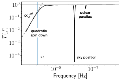
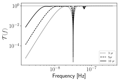
Note that fitting to the sky position absorbs power at and around a frequency of 1/year, corresponding to the Earth’s yearly orbital motion around the Sun. Fitting to the pulsar distance absorbs power at a frequency of 2/year, which corresponds to a parallax measurement. The quadratic spin-down parameter fit acts as a high-pass filter, absorbing frequencies substantially below $1/T$, where $T$ is the time span of the data. The effect of the observing time on the shape of the transmission function is shown in Figure 2.

Pulsars in binaries famously have additional components to the timing model that take into account the various Doppler shifts due to binary motion and relativistic effects, if the line-of-sight passes by the companion (Shapiro delay) or if the binary is in a tight enough orbit to observe the loss of power due to GWs Taylor and Weisberg (1982). These components of the timing model have a minimal effect on sensitivity curves for GWs as the frequencies in question are much higher than those of the sources for which PTAs are searching. We do not include these components when simulating pulsar design matrices, but we will see the (mostly subtle) changes they make when looking at the design matrices of real pulsar data.

Finally, we note that one can also calculate an analogous transmission function associated with the post-fit timing residuals $\delta t^{\rm post}\equiv R\,\delta t$. One finds

$$\sigma^{2}_{\rm post}=\int_{0}^{\infty}{\rm d}f\>{\cal T}_{R}(f)P(f)\,,$$ (14)

where

$${\cal T}_{R}(f)\equiv\frac{1}{N}\sum_{k,l}R_{kl}\,e^{i2\pi f(t_{k}-t_{l})}\,.$$ (15)

This $R$-matrix transmission function was originally described in Blandford et al. (1984), although from a slightly different perspective. In Appendix A, we cast the approach of Blandford et al. (1984) into the more modern $R$-matrix notation.

II.4 Inverse-noise-weighted transmission function

It turns out that there is another way of obtaining a quantity that behaves like a transmission function by working directly with the TMM likelihood (9). The argument of the exponential can be written as $-\frac{1}{2}\chi^{2}$, where

$$\chi^{2}\equiv(\delta t-h(\theta))^{T}G(G^{T}CG)^{-1}G^{T}(\delta t-h(\theta))\,.$$ (16)

If we write this in the Fourier domain by substituting

$$h_{k}(\theta)\equiv h(t_{k};\theta)=\int_{-f_{\rm Nyq}}^{f_{\rm Nyq}}{\rm d}f\>\tilde{h}(f;\theta)\,e^{i2\pi ft_{k}}\,,$$ (17)

where $t_{k}\equiv k\Delta t$ and $f_{\rm Nyq}\equiv 1/(2\Delta t)$, we find

$$\chi^{2}=2T\int_{-f_{\rm Nyq}}^{f_{\rm Nyq}}{\rm d}f\int_{-f_{\rm Nyq}}^{f_{\rm Nyq}}{\rm d}f^{\prime}\>(\widetilde{\delta t}(f)-\tilde{h}(f;\theta))\\ \times{\cal N}^{-1}(f,f^{\prime})(\widetilde{\delta t}{}^{*}(f^{\prime})-\tilde{h}^{*}(f^{\prime};\theta))\,,$$ (18)

where

$${\cal N}^{-1}(f,f^{\prime})\\ \equiv\frac{1}{2T}\sum_{k,l}e^{i2\pi ft_{k}}\,[G(G^{T}CG)^{-1}G^{T}]_{kl}\,e^{-i2\pi f^{\prime}t_{l}}\,.$$ (19)

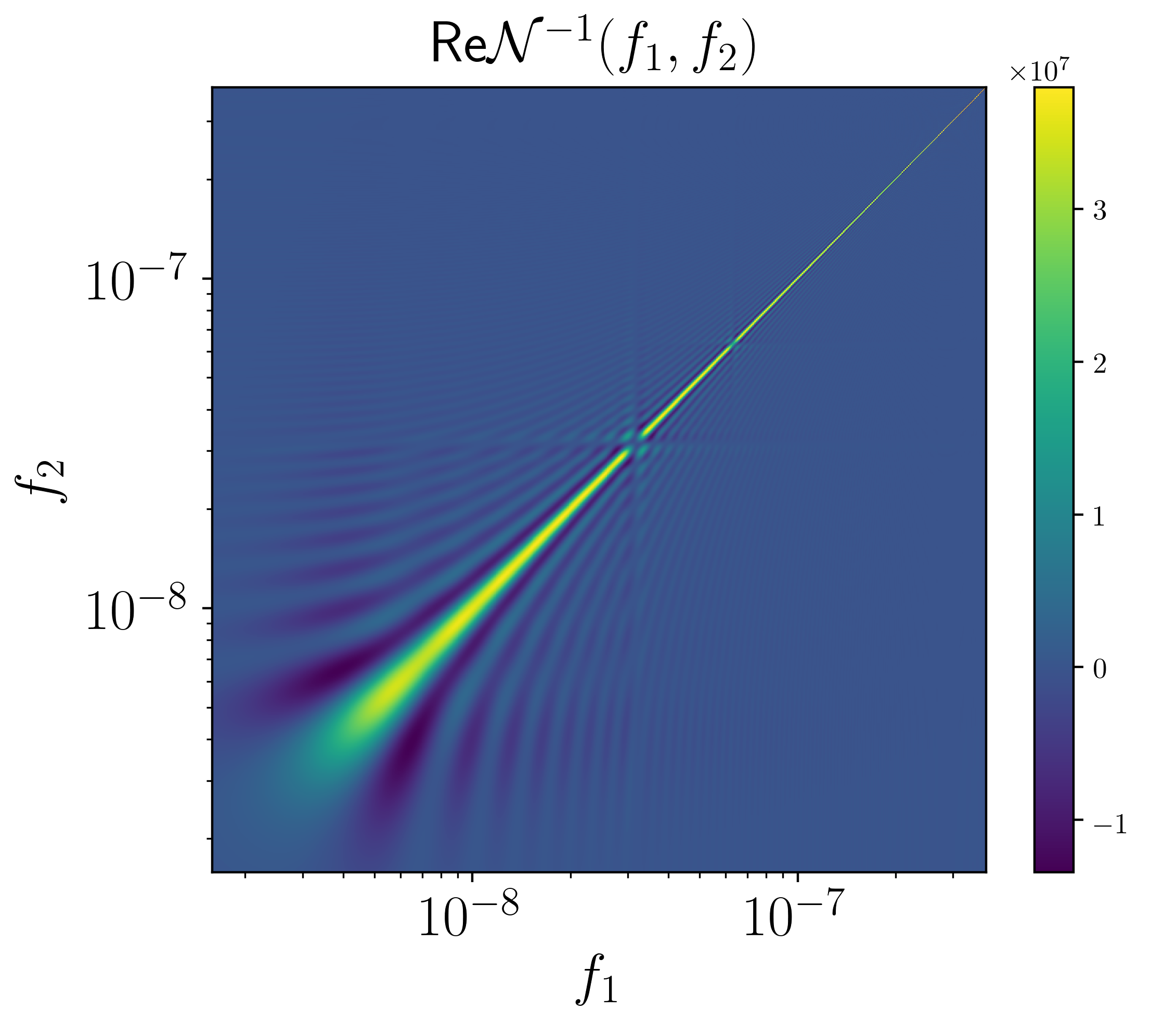
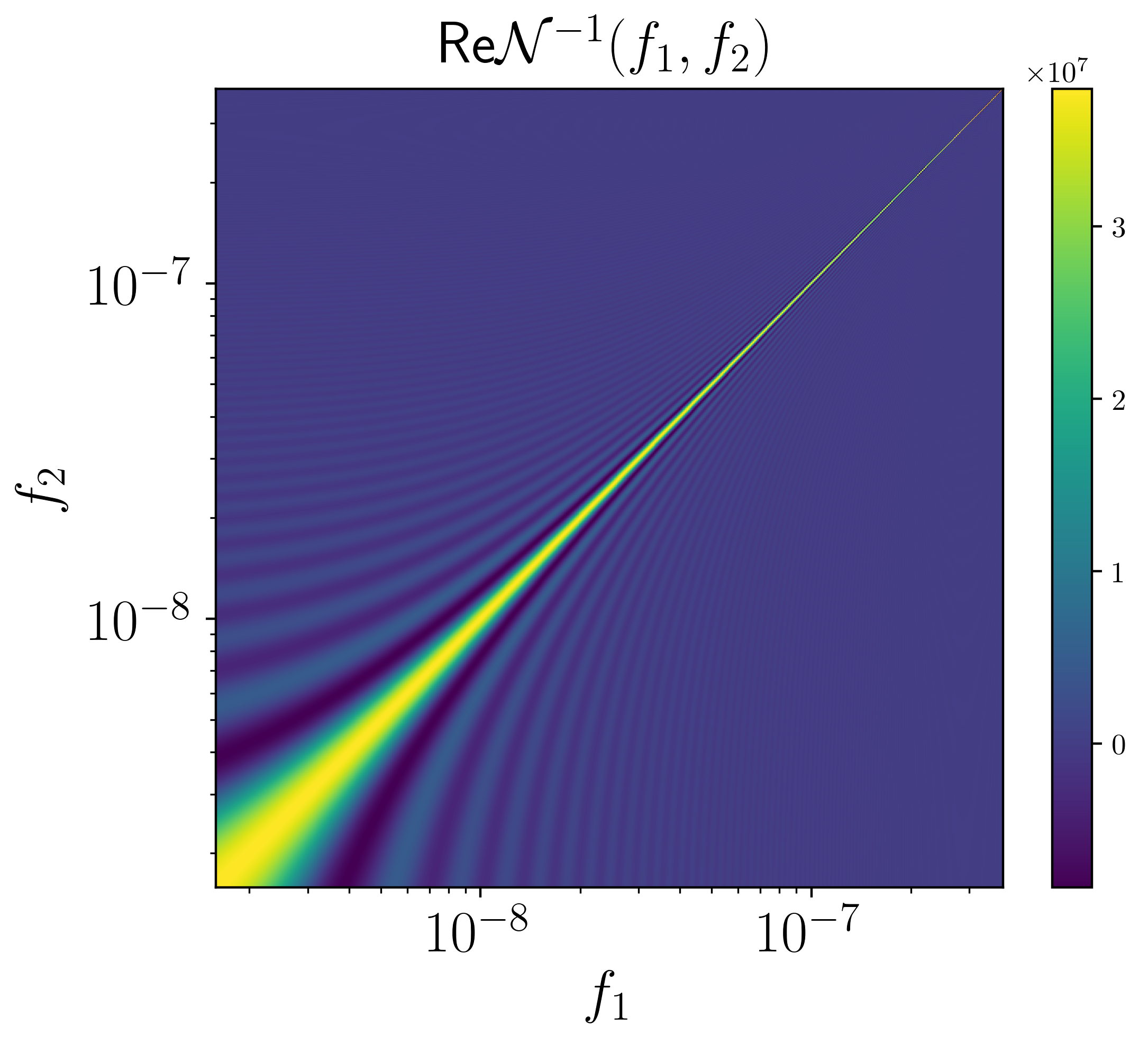
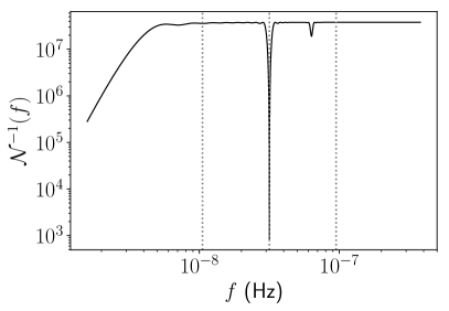
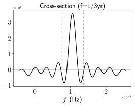
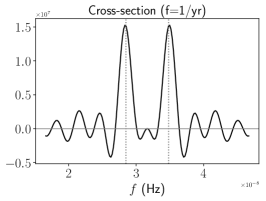
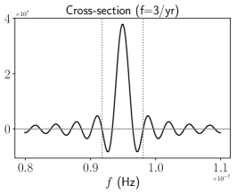
The quantity ${\cal N}^{-1}(f,f^{\prime})$ is a function of two frequencies, $(f,f^{\prime})$, but it turns out to be diagonally-dominated, with the majority of its support on the diagonal $f=f^{\prime}$, as shown in Figure 3. (The broadening of the diagonal band at low frequencies is an artefact of using log-scale axes for the frequencies.) The diagonal component

$${\cal N}^{-1}(f)\equiv\frac{1}{2T}\sum_{k,l}[G(G^{T}CG)^{-1}G^{T}]_{kl}\,e^{i2\pi f(t_{k}-t_{l})}\,,$$ (20)

and three off-diagonal cross-sections of ${\cal N}^{-1}(f,f^{\prime})$ are shown in Figure 4. (The fact that the off-diagonal cross-sections are curved in panel (a) of Figure 4 is again due to using log-scale axes for the frequencies.)

Figure 3: Two-dimensional plot of the real part of the function ${\cal N}^{-1}(f_{1},f_{2})$ for $f_{1},f_{2}>0$ plotted on log-scale axes. Panel (a): ${\rm Re}[{\cal N}^{-1}(f_{1},f_{2})]$ for white noise ($C$ is proportional to the identity matrix) and a fit to the simple quadratic spin-down timing model described in the main text. The small amplitude in the bottom-left hand corner of the plot is due to the absorption of power by the timing model fit at and below $1/T$. There is also suppression at $f_{1}=f_{2}=1/{\rm yr}$ and $f_{1}=f_{2}=2/{\rm yr}$. Panel (b): For comparison, a two-dimensional plot of ${\rm Re}[{\cal N}^{-1}(f_{1},f_{2})]$ for white noise, but without performing a timing model fit (so $G$ is proportional to the identity matrix).

Figure 4: Diagonal and off-diagonal cross-sections of ${\cal N}^{-1}(f_{1},f_{2})$. Panel (a): ${\rm Re}[{\cal N}^{-1}(f_{1},f_{2})]$ from Figure 3 with off-diagonal cross-sections shown by white-dotted lines. Panel (b): Diagonal component ${\cal N}^{-1}(f)$ (the dotted vertical lines show the frequencies of the off-diagonal cross-sections). Panels (c)-(e): Real part of the off-diagonal cross sections of ${\cal N}^{-1}(f_{1},f_{2})$ for $f=1/(3\leavevmode\nobreak\ {\rm yr})$, $f=1/{\rm yr}$, and $f=3/{\rm yr}$. Away from 1/yr, the off-diagonal cross-sections are proportional to Dirichlet sinc functions (the dotted vertical lines indicate off-sets of $\pm 1/T$).

A few remarks are in order:

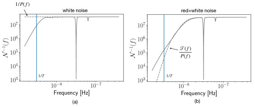
(i) For this particular example, the diagonal component ${\cal N}^{-1}(f)$ is identical in shape with the transmission function ${\cal T}(f)$ shown in Figure 2. The amplitude of ${\cal N}^{-1}(f)$ differs from ${\cal T}(f)$ by a constant factor $1/P(f)=1/(2\sigma^{2}\,\Delta t)$, corresponding to a white noise covariance matrix. Thus, for white noise

$${\cal N}^{-1}(f)={{\cal T}(f)}/{P(f)}\,.$$ (21)

This is illustrated in Figure 5(a). If we also include red noise in the noise covariance matrix $C$ by taking

$$C_{ij}=\int_{0}^{f_{\rm Nyq}}{\rm d}f\>\cos[2\pi f(t_{i}-t_{j})]\,P(f)\,,$$ (22)

$$P(f)=2\sigma^{2}\,\Delta t+Af^{-\gamma}\,,\qquad\gamma>0\,,$$ (23)

then the relationship between ${\cal N}^{-1}(f)$ and ${\cal T}(f)/P(f)$ is only approximate,

$${\cal N}^{-1}(f)\approx{{\cal T}(f)}/{P(f)}\,.$$ (24)

This is illustrated in Figure 5(b).

Figure 5: Plots of the inverse-noise-weighted transmission function ${\cal N}^{-1}(f)$ for the simple quadratic spin-down model described in the main text, and for white noise (a) and red+white noise (b). Panel (a): For white noise, the amplitude of ${\cal N}^{-1}(f)$ is set by the constant value of $1/P(f)$ indicated by the horizontal dashed line. Panel (b): The curved dashed line is a plot of ${\cal T}(f)/P(f)$, which is an approximation to ${\cal N}^{-1}(f)$ for $P(f)$ consisting of red+white noise.

(ii) Away from the dip at 1/yr, where there is suppression of power due to the timing model fit to the pulsar sky position, the off-diagonal cross-sections are proportional to Dirichlet sinc functions

$${\cal D}_{N}((f-f^{\prime})\Delta t)\equiv\frac{1}{N}\frac{\sin[N\pi(f-f^{\prime})\Delta t]}{\sin[\pi(f-f^{\prime})\Delta t]}\,.$$ (25)

When multiplied by $T$, a Dirichlet sinc function can be thought of as finite-time approximation to the Dirac delta function—i.e., $\delta(f-f^{\prime})\simeq T{\cal D}_{N}((f-f)^{\prime}\Delta t)$. Dirichlet sinc functions arise when taking the Fourier transform of a discretely-sampled rectangular window of duration $T=N\Delta t$, see e.g., Romano and Cornish (2017). This diagonally-dominated behavior is what you would expect for ${\cal N}^{-1}(f,f^{\prime})$ if one had only Gaussian-stationary noise. This is the case if one doesn’t have to fit a timing model (Figure 3). Then one can simply replace $G$ by the identity matrix, for which

$${\cal N}^{-1}(f,f^{\prime}) =\frac{1}{2T}\sum_{k,l}e^{i2\pi ft_{k}}[C^{-1}]_{kl}\,e^{-i2\pi f^{\prime}t_{l}}$$ (26)

$$\simeq P^{-1}(f)\,\delta_{ff^{\prime}}\,.$$

The approximate equality in the above equation is a consequence of the Karhunen-Loeve theorem, which states that the discrete Fourier transform operation defined by the unitary matrix $U_{jk}\equiv\frac{1}{N}e^{-i2\pi jk/N}$ approximately diagonalizes a stationary covariance matrix in the limit that the observation time $T=N\,\Delta t$ is much larger than the correlation time of the noise.

(iii) Since fitting to a timing model introduces non-stationarities into the TMM residuals van Haasteren and Levin (2013), one cannot directly appeal to the Karhunen-Loeve theorem for the general expression (19). One needs to explicitly check the validity of the diagonal approximation for ${\cal N}^{-1}(f,f^{\prime})$ as we have done in Figures 3 and 4. We have also numerically computed the sum of ${\cal N}^{-1}(f,f^{\prime})$ over the full two-dimensional array of frequencies $(f,f^{\prime})$ and compared that to the sum of ${\cal N}^{-1}(f,f^{\prime})$ just along the diagonal $f=f^{\prime}$. Even for the more challenging case of a red+white noise covariance matrix (Figure 5(b)) and a fit to the our quadratic spin-down model, the two summations agree to within $\approx 6\%$.

III Timing residual response to gravitational waves

To proceed further in our calculation of pulsar timing sensitivity curves, we need to describe in more detail the timing residual response of a pulsar to an incident GW. We will consider both deterministic and stochastic sources of GWs. Interested readers should see Blandford et al. (1984); Demorest (2007); van Haasteren et al. (2009); Coles et al. (2011); van Haasteren and Levin (2013) for more details.

III.1 Response to a single deterministic source

We will start by writing down the metric perturbations $h_{ab}(t,\vec{x})$ for a single deterministic source emitting plane GWs in the direction $\hat{k}$ (Figure 6). To do this we introduce two coordinate frames: one associated with the solar system barycenter (SSB) and the other associated with the propagation of the GW. We will assume that the source has a symmetry axis (e.g., the direction of the orbital angular momentum vector $\vec{L}$ for a binary system), and that the symmetry axis makes an angle $\iota$ with respect to the line of sight $\hat{k}$ from the GW source to the solar system barycenter, and an angle $\psi$ with respect to the vector $\hat{l}$ when projected onto the plane perpendicular to $\hat{k}$ (Figure 7).

Figure 6: Definition of the unit vectors $\hat{k}$, $\hat{l}$, $\hat{m}$. The direction of propagation of the GW, $\hat{k}$, is opposite the direction to the source, $\hat{n}$. The unit vectors $\hat{l}$, $\hat{m}$ are in the plane perpendicular to $\hat{k}$, and point in directions of constant declination and right ascension, respectively.

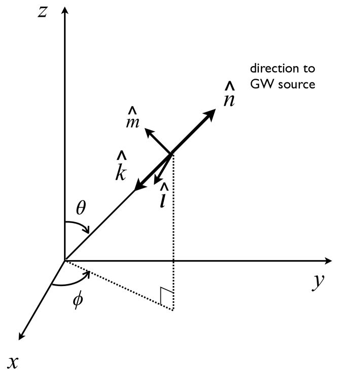
The vectors $\hat{k}$, $\hat{l}$, $\hat{m}$ are defined in the solar system barycenter frame by

$$\hat{k} =(-\sin\theta\,\cos\phi,-\sin\theta\,\sin\phi,-\cos\theta)\equiv-\hat{r}\,,$$ (27)

$$\hat{l} =(\sin\phi,-\cos\phi,0)\equiv-\hat{\phi}\,,$$

$$\hat{m} =(-\cos\theta\,\cos\phi,-\cos\theta\,\sin\phi,\sin\theta)\equiv-\hat{\theta}\,,$$

where $(\theta,\phi)$ are the standard polar and azimuthal angles on the 2-sphere in equatorial coordinates, and the origin of coordinates is at the solar system barycenter. The right ascension $\alpha$ and declination $\delta$ of a source are given in terms of $\theta$ and $\phi$ by $\alpha=\phi$ and $\delta=\pi/2-\theta$.

Figure 7: Relation between the unit vectors $\hat{l}$, $\hat{m}$ and $\hat{u}$, $\hat{v}$. Definition of: (a) inclination angle $\iota$, and (b) polarization angle $\psi$. Here $\vec{L}$ is the angular momentum vector and $\hat{k}$ is the propagation direction of the GW. The vectors $\hat{l}$, $\hat{m}$ and $\hat{u}$, $\hat{v}$ are orthogonal unit vectors in the plane perpendicular to $\hat{k}$, defined by (27) and (29), respectively.

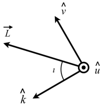
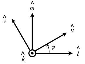
The angles $\iota$ and $\psi$ are the inclination and polarization angles of the source, respectively. They can be written in terms of the unit vectors $\hat{k}$, $\hat{l}$, $\hat{L}\equiv\vec{L}/|\vec{L}|$, and $\hat{u}$ via:

$$\cos\iota\equiv\hat{k}\cdot\hat{L}\,,\qquad\cos\psi\equiv\hat{u}\cdot\hat{l}\,,$$ (28)

where

$$\hat{u}\equiv\frac{\hat{L}\times\hat{k}}{|\hat{L}\times\hat{k}|}\,,\qquad\hat{v}\equiv\hat{k}\times\hat{u}\,,$$ (29)

are two orthogonal unit vectors in the plane perpendicular to $\hat{k}$ (Figure 7). Note that $\iota=0$ or $\pi$ corresponds to the orbital plane being seen face-on or face-off; $\iota=\pi/2$ or $3\pi/2$ corresponds to seing the orbital plane edge on. The unit vectors $\hat{u}$, $\hat{v}$ are related to $\hat{l}$, $\hat{m}$ by a rotation around $\hat{k}$ through the angle $\psi$ as shown in Figure 7.

From $\hat{u}$ and $\hat{v}$, we can construct a preferred set of polarization tensors:

$$\epsilon^{+}_{ab}(\hat{k},\psi) \equiv\hat{u}_{a}\hat{u}_{b}-\hat{v}_{a}\hat{v}_{b}\,,$$ (30)

$$\epsilon^{\times}_{ab}(\hat{k},\psi) \equiv\hat{u}_{a}\hat{v}_{b}+\hat{v}_{a}\hat{u}_{b}\,.$$

Using these polarization tensors, we can expand the metric perturbations:

$$h_{ab}(t,\vec{x})=h_{+}(t-\hat{k}\cdot\vec{x}/c;\iota)\epsilon^{+}_{ab}(\hat{k},\psi)\\ +h_{\times}(t-\hat{k}\cdot\vec{x}/c;\iota)\epsilon^{\times}_{ab}(\hat{k},\psi)$$ (31)

or, equivalently,

$$h_{ab}(t,\vec{x})=\int_{-\infty}^{\infty}{\rm d}f\>\left[\tilde{h}_{+}(f;\iota)\epsilon^{+}_{ab}(\hat{k},\psi)\right.\\ \left.+\tilde{h}_{\times}(f;\iota)\epsilon^{\times}_{ab}(\hat{k},\psi)\right]\,e^{i2\pi f(t-\hat{k}\cdot\vec{x}/c)}\,,$$ (32)

where $\tilde{h}_{+,\times}(f;\iota)$ are the Fourier transforms of $h_{+,\times}(t;\iota)$. The timing residual response of a pulsar to such a deterministic GW is then Detweiler (1979):

$$h(t;\hat{k},\iota,\psi)=\int_{-\infty}^{\infty}{\rm d}f\>\tilde{h}(f;\hat{k},\iota,\psi)\,e^{i2\pi ft}\,,$$ (33)

where

$$\tilde{h}(f;\hat{k},\iota,\psi)=R^{+}(f,\hat{k},\psi)\tilde{h}_{+}(f;\iota)\\ +R^{\times}(f,\hat{k},\psi)\tilde{h}_{\times}(f;\iota)\,,$$ (34)

with

$$R^{+,\times}(f,\hat{k},\psi)\equiv\frac{1}{i2\pi f}\frac{1}{2}\frac{\hat{p}^{a}\hat{p}^{b}}{1+\hat{p}\cdot\hat{k}}\epsilon^{+,\times}_{ab}(\hat{k},\psi)\\ \times\left(1-e^{-i2\pi fD(1+\hat{k}\cdot\hat{p})/c}\right)\,.$$ (35)

Here $\hat{p}^{a}$ is a unit vector pointing from the solar system barycenter to the pulsar, and $D$ is the distance to the pulsar. The function $R^{+,\times}(f,\hat{k},\psi)$ is the timing residual response function of a pulsar to a monochromatic plane GW propagating in direction $\hat{k}$, with frequency $f$, polarization $+,\times$, and polarization angle $\psi$. The two terms in the response function are called the ‘Earth term’ and ‘pulsar term’, respectively, since they involve sampling the GW phase at Earth and at the location of the pulsar, a distance $D$ away from Earth. The factor of $1/(i2\pi f)$ comes from the fact that we are working with timing residuals, as opposed to Doppler shifts in the pulse frequency.

For the analyses that we will do in this paper, we will typically ignore the pulsar-term contribution to the timing residual response to GWs, as this term will not contribute to the cross-power when correlating the signal associated with distinct pulsars. (The separation between pulsars ($\sim{\rm kpc}$) is much greater the wavelengths of the GWs that we are sensitive to, which are of order $\lesssim 10\leavevmode\nobreak\ {\rm lyr}$.) There is a contribution, however, to the auto-correlated power for a single pulsar, which comes from the exponential part of $|R^{+,\times}(f,\hat{k},\psi)|^{2}$:

$$\left|1-e^{-i2\pi fD(1+\hat{k}\cdot\hat{p})/c}\right|^{2}\\ =2\left[1-\cos(2\pi fD(1+\hat{k}\cdot\hat{p})/c)\right]\simeq 2\,,$$ (36)

where we have ignored the cosine term since it is a rapidly-oscillating function of the GW propagation direction $\hat{k}$, and hence does not contribute significantly when summed over the sky. The value ‘2’ corresponds to the sum of the Earth-Earth and pulsar-pulsar auto-correlation terms.

III.1.1 Circular binaries

To proceed further, we need to specify the form of $h_{+,\times}(t;\iota)$ or its Fourier transform $\tilde{h}_{+,\times}(f;\iota)$. For example, for a circular binary

$$h_{+}(t;\iota) =h_{0}(t)\left(\frac{1+\cos^{2}\iota}{2}\right)\,\cos 2\Phi(t)\,,$$ (37)

$$h_{\times}(t;\iota) =h_{0}(t)\,\cos\iota\,\sin 2\Phi(t)\,,$$

where $\Phi(t)$ is the orbital phase and $h_{0}(t)$ is a dimensionless amplitude given by

$$h_{0}(t)=\frac{4c}{D_{L}}\left(\frac{G\mathcal{M}_{\rm c}}{c^{3}}\right)^{5/3}\omega(t)^{2/3}\,.$$ (38)

Here $D_{L}$ is the luminosity distance to the source, $\mathcal{M}_{\rm c}\equiv(m_{1}m_{2})^{3/5}/(m_{1}+m_{2})^{1/5}$ is the chirp mass of the binary system, and $\omega(t)$ is the instantaneous orbital angular frequency, $\Phi(t)=\int^{t}{\rm d}t^{\prime}\>\omega(t^{\prime})$. For an evolving binary system

$$\frac{{\rm d}\omega}{{\rm d}t}=\frac{96}{5}\left(\frac{G\mathcal{M}_{c}}{c^{3}}\right)^{5/3}\omega(t)^{11/3}\,,$$ (39)

which is a consequence of energy balance between the radiated power in GWs and the orbital energy lost by the binary system. The instantaneous GW frequency $f(t)$ is related to the orbital frequency $\omega(t)$ via $\omega(t)=\pi f(t)$.

The above differential equation for $\omega(t)$ (or, equivalently, for $f(t)$) can be integrated to yield

$$f(\tau)=\frac{1}{\pi}\left(\frac{G\mathcal{M}_{c}}{c^{3}}\right)^{-5/8}\left(\frac{5}{256}\frac{1}{\tau}\right)^{3/8}\,,$$ (40)

where $\tau\equiv t_{\rm col}-t$ is the time to coalescence. Inverting (40), we obtain

$$\tau=\frac{5}{256}\left(\frac{G\mathcal{M}_{c}}{c^{3}}\right)^{-5/3}\left(\pi f\right)^{-8/3}\,,$$ (41)

which is the time to coalescence for a binary system currently having GW frequency $f$. Note that for a SMBH binary with $10^{9}$ solar-mass BHs (which is the primary source for PTAs) and GW frequency $f=8\leavevmode\nobreak\ {\rm nHz}$ (which is one of the most sensitive frequencies for the current decade-long PTA searches), the time to coalescence is $\tau\sim 10^{5}\leavevmode\nobreak\ {\rm yr}$, which is four orders of magnitude larger than a decade-long observation $T=10\leavevmode\nobreak\ {\rm yr}$. Over the course of the observation the change in the GW frequency for the above SMBH binary is

$$\Delta f\simeq\frac{1}{\pi}\left(\frac{G\mathcal{M}_{c}}{c^{3}}\right)^{-5/8}\left(\frac{5}{256}\frac{1}{\tau}\right)^{3/8}\,\frac{3}{8}\frac{T}{\tau}\approx 3\times 10^{-13}\leavevmode\nobreak\ {\rm Hz}\,,$$ (42)

which is four orders of magnitude smaller than the frequency bin width $1/T$, set by the total observation time $T$. Thus, for the purposes of this paper, we will take our deterministic source to be a monochromatic binary with $f(\tau)=f_{0}={\rm const}$.

With this simplification, equations (37) and (38) become

$$h_{+}(t;\iota,\phi_{0}) =h_{0}\left(\frac{1+\cos^{2}\iota}{2}\right)\,\cos(2\pi f_{0}t+\phi_{0})\,,$$ (43)

$$h_{\times}(t;\iota,\phi_{0}) =h_{0}\cos\iota\,\sin(2\pi f_{0}t+\phi_{0})\,,$$

where $\phi_{0}$ is the initial phase and $h_{0}$ is the (constant) strain amplitude

$$h_{0}=\frac{4c}{D_{L}}\left(\frac{G\mathcal{M}_{\rm c}}{c^{3}}\right)^{5/3}(\pi f_{0})^{2/3}\,.$$ (44)

The Fourier transforms of $h_{+,\times}(t;\iota,\phi_{0})$ are then

$$\tilde{h}_{+}(f;\iota,\phi_{0}) =h_{0}\left(\frac{1+\cos^{2}\iota}{2}\right)$$ (45)

$$\qquad\times\frac{1}{2}\left[e^{i\phi_{0}}\delta(f-f_{0})+e^{-i\phi_{0}}\delta(f+f_{0})\right]\,,$$

$$\tilde{h}_{\times}(f;\iota,\phi_{0}) =h_{0}\cos\iota\,$$

$$\qquad\times\frac{1}{2i}\left[e^{i\phi_{0}}\delta(f-f_{0})-e^{-i\phi_{0}}\delta(f+f_{0})\right]\,.$$

But since the signals are observed for only a finite duration, the Dirac delta functions $\delta(f\mp f_{0})$ should be replaced by their finite-time equivalents $\delta_{T}(f\mp f_{0})$ defined by

$$\delta_{T}(f)\equiv\int_{-T/2}^{T/2}{\rm d}t\>e^{-i2\pi ft}=\frac{\sin(\pi fT)}{\pi f}\equiv T\,{\rm sinc}(\pi fT)\,,$$ (46)

where $T$ is the observation time for the pulsar. If one wants to also include the discreteness $\Delta t$ of the time-series data, then the Dirac delta functions should be replaced by Dirichlet sinc functions, $T\mathcal{D}_{N}[(f\mp f_{0})\Delta t]$ (see (25)). It turns out that the final (approximate) expressions that we obtain, cf. (48) and (52), are independent of which finite-time approximation we use.

III.1.2 Averaging over inclination, polarization, and sky position

Using the above expressions for $\tilde{h}_{+,\times}(f;\iota,\phi_{0})$ and (35) for $R^{+,\times}(f,\hat{k},\psi)$, we can calculate the squared response $|\tilde{h}(f)|^{2}$ averaged over the inclination of the source (defined by the inclination and polarization angles $\iota$ and $\psi$), initial phase $\phi_{0}$, and sky direction $\hat{n}\equiv-\hat{k}$. This is relevant for the case where these quantities are not known a priori. Defining

$$|\tilde{h}(f;\hat{k})|^{2}\equiv\frac{1}{2\pi}\int_{0}^{2\pi}{\rm d}\phi_{0}\>\left(\frac{1}{4\pi}\int_{0}^{2\pi}{\rm d}\psi\>\right.\\ \times\left.\int_{-1}^{1}\>{\rm d}(\cos\iota)\,|\tilde{h}(f;\hat{k},\iota,\psi,\phi_{0})|^{2}\right)\,,$$ (47)

it is fairly easy to show that

$$\frac{2|\tilde{h}(f;\hat{k})|^{2}}{T}\simeq\frac{4}{5}\mathcal{R}(f,\hat{k})S_{h}(f)$$ (48)

where

$$\mathcal{R}(f,\hat{k})\equiv\frac{1}{2}\left(|R^{+}(f,\hat{k},0)|^{2}+|R^{\times}(f,\hat{k},0)|^{2}\right)\,,$$ (49)

$$S_{h}(f)\equiv\frac{1}{2}\,{h_{0}^{2}}\left[\delta(f-f_{0})+\delta(f+f_{0})\right]\,.$$ (50)

The factor of $4/5$ in (48) comes from the average over inclination angles $(\iota,\psi)$; $\mathcal{R}(f,\hat{k})$ encodes the timing residual response of a pulsar to a plane GW propagating in direction $\hat{k}$ averaged over the $(+,\times)$ polarizations and the polarization angle $\psi$; and $S_{h}(f)$ is the strain power-spectral density of a monochromatic GW having frequency $f_{0}$. The approximate equality in (48) is there because we made the approximation $\delta_{T}^{2}(f\mp f_{0})\simeq T\delta(f\mp f_{0})$ for the product of two finite-time Dirac delta functions. This allows us to write $S_{h}(f)$ in terms of ordinary Dirac delta functions, which are formally singular at $f=\pm f_{0}$. But this is not a problem, as $S_{h}(f)$ will only need to be evaluated under an integral sign for the expected signal-to-noise ratio calculations that we will perform in Section IV.1. This approximation gives answers that are good to within $\lesssim 10\%$ for noise power spectral densities that don’t vary significantly over a frequency bandwidth $\Delta f\sim 1/T$ in the neighboorhood of $\pm f_{0}$.

If we also average over sky location, defining

$$|\tilde{h}(f)|^{2}\equiv\frac{1}{4\pi}\int{\rm d}^{2}\Omega_{\hat{k}}\>\left(\frac{1}{2\pi}\int_{0}^{2\pi}{\rm d}\phi_{0}\>\right.\\ \left.\times\left(\frac{1}{4\pi}\int_{0}^{2\pi}{\rm d}\psi\>\int_{-1}^{1}\>{\rm d}(\cos\iota)\,|\tilde{h}(f;\hat{k},\iota,\psi,\phi_{0})|^{2}\right)\right)\,,$$ (51)

we find

$$\frac{2|\tilde{h}(f)|^{2}}{T}\simeq\frac{4}{5}\mathcal{R}(f)S_{h}(f)$$ (52)

where

$$\mathcal{R}(f) \equiv\frac{1}{8\pi}\int{\rm d}^{2}\Omega_{\hat{k}}\>\left(|R^{+}(f,\hat{k},0)|^{2}+|R^{\times}(f,\hat{k},0)|^{2}\right)$$ (53)

$$=\frac{1}{12\pi^{2}f^{2}}\,.$$

Note that the expression for ${\cal R}(f)$ is independent of the direction $\hat{p}$ to the pulsar. The above expressions will be used later on when defining the detection sensitivity curves in Section IV.

III.2 Response to a stochastic GW background

For a stochastic GW background, the metric perturbations can be written as a superposition of plane GWs having different frequencies $f$, polarizations $\{+,\times\}$, and propagation directions $\hat{k}$:

$$h_{ab}(t,\vec{x})=\int{\rm d}^{2}\Omega_{\hat{k}}\>\int_{-\infty}^{\infty}{\rm d}f\>\left[\tilde{h}_{+}(f,\hat{k})e^{+}_{ab}(\hat{k})\right.\\ \left.+\tilde{h}_{\times}(f,\hat{k})e^{\times}_{ab}(\hat{k})\right]e^{i2\pi f(t-\hat{k}\cdot\vec{x}/c)}\,,$$ (54)

where $e^{+,\times}_{ab}(\hat{k})\equiv\epsilon^{+,\times}_{ab}(\hat{k},0)$. This is basically (32) but allowing for contributions from different propagation direction $\hat{k}$. Since we will assume that the sources producing the GW background have no preferred polarization direction or symmetry axis, we have set $\psi=0$ and $\iota=0$ in the expansion for $h_{ab}(t,\vec{x})$. The timing residual response of a pulsar to the background is then

$$h(t)=\int_{-\infty}^{\infty}{\rm d}f\>\tilde{h}(f)e^{i2\pi ft}\,,$$ (55)

where

$$\tilde{h}(f)=\int{\rm d}^{2}\Omega_{\hat{k}}\>\left[R^{+}(f,\hat{k},0)\tilde{h}_{+}(f;\hat{k})\right.\\ \left.+R^{\times}(f,\hat{k},0)\tilde{h}_{\times}(f;\hat{k})\right]$$ (56)

with $R^{+,\times}(f,\hat{k},0)$ given by (35). As discussed there, we will generally ignore the contribution of the pulsar term to the response function, except when calculating the auto-correlated power, which will have contributions from both the Earth-Earth and pulsar-pulsar auto-correlation terms.

The Fourier components $\tilde{h}_{+,\times}(f;\hat{k})$ that enter the plane-wave expansion of the metric perturbations are random fields. Their quadratic expectation values completely define the statistical properties of the background, under the assumption that it is Gaussian-distributed. For simplicity, we will assume that the GW background is stationary, unpolarized, and isotropic, for which $\langle\tilde{h}_{P}(f;\hat{k})\rangle=0$ and

$$\langle\tilde{h}_{P}(f;\hat{k})\tilde{h}_{P^{\prime}}^{*}(f^{\prime};\hat{k}^{\prime})=\frac{1}{16\pi}S_{h}(f)\delta(f-f^{\prime})\delta_{PP^{\prime}}\delta^{2}(\hat{k},\hat{k}^{\prime})\,,$$ (57)

where $P=\{+,\times\}$. Here $S_{h}(f)$ is the (one-sided) strain power spectral density of the background (units of ${\rm strain}{}^{2}/{\rm Hz}$), which is related to the dimensionless energy-density spectrum $\Omega_{\rm gw}(f)$ via

$$S_{h}(f)=\frac{3H_{0}^{2}}{2\pi^{2}}\frac{\Omega_{\rm gw}(f)}{f^{3}}\,.$$ (58)

It is also common to describe the background in terms of it dimensionless characteristic strain defined by

$$h_{c}(f)\equiv\sqrt{fS_{h}(f)}=A_{\rm gw}(f/f_{\rm yr})^{\alpha}\,,$$ (59)

where the second equality assumes a power-law form for the background. Note that for a background produced by the cosmological population of SMBH binaries, $\alpha=-2/3$.

III.2.1 GW contribution to the noise covariance matrix

Using the above expressions for the timing residual response of a pulsar to a GW background, we can calculate the GW contribution to the noise covariance matrix when cross-correlating timing residuals associated with two Earth-pulsar baselines $I$ and $J$. Denoting the GW contributions to the two sets of timing residuals as $h_{I}(t)$ and $h_{J}(t)$, respectively, one can show that the covariance matrix is block-diagonal with components

$$C_{h,IJ}\equiv\langle h_{I}h_{J}^{T}\rangle-\langle h_{I}\rangle\langle h_{J}^{T}\rangle=\chi_{IJ}\,C_{h}\,,$$ (60)

where

$$\chi_{IJ}\equiv\frac{1}{2}+\frac{3}{2}\left(\frac{1-\hat{p}_{I}\cdot\hat{p}_{J}}{2}\right)\left[\ln\left(\frac{1-\hat{p}_{I}\cdot\hat{p}_{J}}{2}\right)-\frac{1}{6}\right]\\ +\frac{1}{2}\,\delta_{IJ}\,,$$ (61)

and

$$C_{h,ij}=\int_{0}^{f_{\rm Nyq}}{\rm d}f\>\cos[2\pi f(t_{i}-t_{i})]P_{h}(f)\,,$$ (62)

$$P_{h}(f)={\cal R}(f)S_{h}(f)=\frac{A_{\rm gw}^{2}}{12\pi^{2}}\left(\frac{f}{f_{\rm yr}}\right)^{2\alpha}f^{-3}\,.$$ (63)

The full noise covariance matrix, which includes contributions instrinsic to the pulsar and to the measurement process, is also block-diagonal with components

$$C_{IJ}=\delta_{IJ}C_{n,I}+C_{h,IJ}\,.$$ (64)

Here $C_{n,I}$ is given by (62), but with the pulsar noise power spectral density $P_{n_{I}}(f)$ replacing $P_{h}(f)$. This last equation assumes that the noise contributions associated with different pulsars are not correlated with one another.

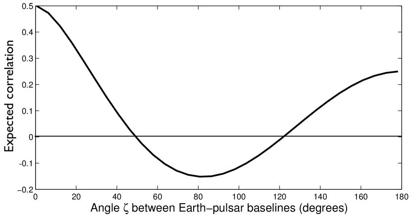
The quantity $\chi_{IJ}\equiv\chi(\zeta_{IJ})$ defined in (61) is the Hellings and Downs factor Hellings and Downs (1983) for a pair of pulsars separated by angle $\zeta_{IJ}=\cos^{-1}(\hat{p}_{I}\cdot\hat{p}_{J})$ (see Figure 8). It arises when cross-correlating the GW-induced timing residuals for an unpolarized, isotropic GW background. Note that $\chi_{IJ}$ has been normalized such that $\chi_{II}=1$ (for a single pulsar).

Figure 8: Hellings and Downs curve. Plotted is the expected correlation for the timing residuals induced in a pair of distinct Earth-pulsar baselines by an unpolarized, isotropic GW background.

IV Sensitivity curves

Ultimately, a detection sensitivity curve should tell us how likely it is to detect a particular type of GW signal. So it should depend not only on the properties of the noise in the detector, but also on the type of signal that one is searching for and the method that one uses to search for it. So here we extend the formalism of the previous two sections to define sensitivity curves for searches for a deterministic GW signal from a circular binary and an unpolarized, isotropic stochastic GW background. We begin by writing down expressions for the optimal detection statistics for these two different sources and their corresponding expected signal-to-noise ratios (SNRs). We will see that from these expected SNRs, we can read off an effective strain-noise power spectral density, which has the interpretation of a detection sensitivity curve.

IV.1 Matched filtering for a deterministic GW signal

For a deterministic GW signal, we can use the method of matched filtering to construct an optimal detection statistic. This method has been used extensively in the PTA literature, Babak et al. (2016); Babak and Sesana (2012); Ellis et al. (2012); Yardley et al. (2010) and is also the basis for the approximate deterministic sensitivity curves in Moore et al. (2015b). Letting $Q_{I}$ denote the filter function for pulsar $I$ (where $I=1,2,\cdots,N_{\rm p}$), we define

$$\hat{\mathcal{S}}\equiv\sum_{I}Q_{I}^{T}r_{I}=\sum_{I}\sum_{\alpha}Q_{I\alpha}r_{I\alpha}\,,$$ (65)

where $r_{I}\equiv G_{I}^{T}\delta t_{I}$ are the TMM residuals for pulsar $I$. The filter function is determined by maximizing the expected signal-to-noise ratio, $\rho\equiv\mu/\sigma$, of $\hat{\mathcal{S}}$. The expectation value of $\hat{\mathcal{S}}$ is given by

$$\mu\equiv\langle\hat{\mathcal{S}}\rangle=\sum_{I}Q_{I}^{T}G_{I}^{T}h_{I}(\theta)$$ (66)

and its variance is given by

$$\sigma^{2}\equiv\langle\hat{\mathcal{S}}^{2}\rangle-\langle\hat{\mathcal{S}}\rangle^{2}=\sum_{I}Q_{I}^{T}\Sigma_{n,I}Q_{I}\,,$$ (67)

where $\Sigma_{n,I}\equiv G_{I}^{T}C_{n,I}G_{I}$ is the noise covariance matrix for $r_{I}$. This result for the variance assumes that the only GW contribution to the timing residuals is from a deterministic GW source, and not from a stochastic GW background. The presence of a stochastic background would contribute to both the diagonal and off-diagonal block matrices (see (64)). In what follows, we will assume that the off-diagonal terms are small compared to the diagonal (auto-correlated) terms. But we will replace $\Sigma_{n,I}$ by $\Sigma_{I}\equiv G_{I}^{T}C_{I}G_{I}$, where $C_{I}\equiv C_{n,I}+C_{h}$, thereby allowing a stochastic background to contribute to the auto-correlated noise (sometimes called GW self-noise).

Using the above results for the mean and variance of $\hat{\mathcal{S}}$, the square of the expected signal-to-noise ratio is

$$\rho^{2}\equiv\frac{\mu^{2}}{\sigma^{2}}=\frac{\sum_{I,J}Q^{T}_{I}\,G^{T}_{I}h_{I}(\theta)Q^{T}_{J}\,G^{T}_{J}h_{J}(\theta)}{\sum_{K}Q_{K}^{T}\Sigma_{K}Q_{K}}\,,$$ (68)

with the optimal filter given by

$$\frac{\delta\rho^{2}}{\delta Q_{I}}=0\quad\Rightarrow\quad Q_{I}=\Sigma_{I}^{-1}G^{T}_{I}h_{I}(\theta)\,.$$ (69)

Note that $Q_{I}$ is a noise-weighted version of the TMM signal waveform, as expected for a matched-filter statistic. Using this expression, the expected signal-to-noise ratio becomes

$$\rho^{2}(\theta) =\sum_{I}h_{I}(\theta)^{T}G_{I}\Sigma_{I}^{-1}G_{I}^{T}h_{I}(\theta)$$ (70)

$$=\sum_{I}h_{I}(\theta)^{T}G_{I}(G^{T}_{I}C_{I}G_{I})^{-1}G_{I}^{T}h_{I}(\theta)\,.$$

This last expression can be evaluated in the frequency domain by using (19) for ${\cal N}_{I}^{-1}(f,f^{\prime})$ and restricting to the diagonal component ${\cal N}^{-1}(f)$ as discussed in Section II.4:

$$\rho^{2}(\theta)\simeq 4\int_{0}^{f_{\rm Nyq}}{\rm d}f\>\sum_{I}|\tilde{h}_{I}(f;\theta)|^{2}\,{\cal N}_{I}^{-1}(f)\,.$$ (71)

Recall that $\theta$ denote the set of GW parameters. For the case of a circular binary discussed in Section III.1.1, $\theta=\{\hat{k},\iota,\psi,\phi_{0}\}$.

IV.1.1 Detection sensitivity curve for sky and inclination-averaged sources

To proceed further, we first consider the case of GWs from a single binary system averaged over the initial phase, inclination of the source, as well as its sky location. Using (52) for $|\tilde{h}_{I}(f)|^{2}$, we have

$$\langle\rho^{2}\rangle_{\rm inc,\,sky} \simeq 4\int_{0}^{f_{\rm Nyq}}{\rm d}f\>\sum_{I}\frac{T_{I}}{2}\frac{4}{5}\mathcal{R}(f)S_{h}(f)\,\mathcal{N}_{I}^{-1}(f)$$ (72)

$$=2T_{\rm obs}\int_{0}^{f_{\rm Nyq}}{\rm d}f\>\frac{S_{h}(f)}{S_{\rm eff}(f)}\,,$$

where

$${S_{\rm eff}(f)}\equiv\left(\frac{4}{5}\sum_{I}\frac{T_{I}}{T_{\rm obs}}\frac{1}{S_{I}(f)}\right)^{-1}\,,$$ (73)

$$S_{I}(f)\equiv\frac{1}{\mathcal{N}^{-1}_{I}(f)\mathcal{R}(f)}\,.$$ (74)

Here, $S_{I}(f)$ is the strain-noise power spectral density for pulsar $I$, and $S_{\rm eff}(f)$ is an effective strain noise power spectral density for an array of pulsars. Given how $S_{\rm eff}(f)$ appears in the expression for the expected signal-to-noise ratio, we will use it, or its dimensionless characteristic strain,

$$h_{\rm eff}(f)\equiv\sqrt{fS_{\rm eff}(f)}\,$$ (75)

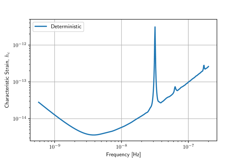
as a sensitivity curve for detecting a deterministic GW source averaged over its initial phase, inclination, and sky location. A plot of $S_{\rm eff}(f)$ for the array of pulsars in the NANOGrav 11-year data Arzoumanian et al. (2018) is shown in Figure 9.

Figure 9: Sensitivity curve for a single deterministic GW source averaged over its initial phase, inclination, and sky location. This plot was constructed using the NANOGrav 11-year data.

Note that for a monochromatic source, $S_{h}(f)$ has a very simple form given by (50), which implies

$$\bar{\rho}\equiv\sqrt{\langle\rho^{2}\rangle_{\rm inc,\,sky}}\simeq h_{0}\sqrt{\frac{T_{\rm obs}}{S_{\rm eff}(f_{0})}}\,.$$ (76)

IV.1.2 SNR and characteristic amplitude sky maps for inclination-averaged sources

If we average over initial phase and source inclination, but not over sky location, cf. (48) for $|\tilde{h}_{I}(f,\hat{k})|^{2}$, we obtain

$$\langle\rho^{2}(\hat{k})\rangle_{\rm inc} \simeq 4\int_{0}^{f_{\rm Nyq}}{\rm d}f\>\sum_{I}\frac{T_{I}}{2}\frac{4}{5}\mathcal{R}_{I}(f,\hat{k})S_{h}(f)\,\mathcal{N}_{I}^{-1}(f)$$ (77)

$$=2T_{\rm obs}\int_{0}^{f_{\rm Nyq}}{\rm d}f\>\frac{S_{h}(f)}{S_{\rm eff}(f,\hat{k})}\,,$$

where

$$S_{\rm eff}(f,\hat{k})\equiv\left(\frac{4}{5}\sum_{I}\frac{T_{I}}{T_{\rm obs}}\frac{1}{S_{I}(f,\hat{k})}\right)^{-1}\,,$$ (78)

$$S_{I}(f,\hat{k})\equiv\frac{1}{\mathcal{N}^{-1}_{I}(f)\mathcal{R}_{I}(f,\hat{k})}\,,$$ (79)

with $\mathcal{R}_{I}(f,\hat{k})$ given by (49). These expressions are analogous to (73), but with added dependence on the propagation direction $\hat{k}$ of the GW. It turns out that we can factor out the $\hat{k}$ dependence on the right-hand side of the above expression for $S_{\rm eff}(f,\hat{k})$ if we ignore the frequency-dependent part of the pulsar-term contribution to $|R_{I}^{P}(f,\hat{k},0)|^{2}$, as discussed in the context of (36). Making this approximation,

$$S_{\rm eff}(f,\hat{k})\simeq\left(\frac{12}{5}\sum_{I}\frac{T_{I}}{T_{\rm obs}}\frac{1}{S_{I}(f)}\,\right.\\ \left.\times\left[(F^{+}_{I}(\hat{k}))^{2}+(F^{\times}_{I}(\hat{k}))^{2}\right]\right)^{-1}\,,$$ (80)

where $F_{I}^{+,\times}(\hat{k})$ are defined by

$$F_{I}^{+,\times}(\hat{k})\equiv\frac{1}{2}\frac{\hat{p}_{I}^{a}\hat{p}_{I}^{b}}{1+\hat{p}_{I}\cdot\hat{k}}\,e_{ab}^{+,\times}(\hat{k})\,.$$ (81)

As before, it is easy to do the integral over frequency for a monochromatic source, for which $S_{h}(f)$ is given by (50). The result is

$$\rho(\hat{n})\equiv\sqrt{\langle\rho^{2}(\hat{k})\rangle_{\rm inc}}\simeq h_{0}\sqrt{\frac{T_{\rm obs}}{S_{\rm eff}(f_{0},\hat{k})}}\,,$$ (82)

where the direction $\hat{n}$ of the source on the sky is opposite the direction of GW propagation, $\hat{n}=-\hat{k}$. A plot of $\rho(\hat{n})$ for a pair of $10^{9}$ solar-mass BHs at a luminosity distance of 100 Mpc, emitting monochromatic GWs at the frequency $f_{0}=8\leavevmode\nobreak\ {\rm nHz}$ is shown in Figure 10.

Figure 10: Sky map of the expected matched-filter signal-to-noise ratio $\rho(\hat{n})$ for a monochromatic circular binary (GW frequency $f_{0}=8\leavevmode\nobreak\ {\rm nHz}$) consisting of a pair of $10^{9}$ solar-mass BHs at a luminosity distance of 100 Mpc. This plot was constructed using the NANOGrav 11-year data.

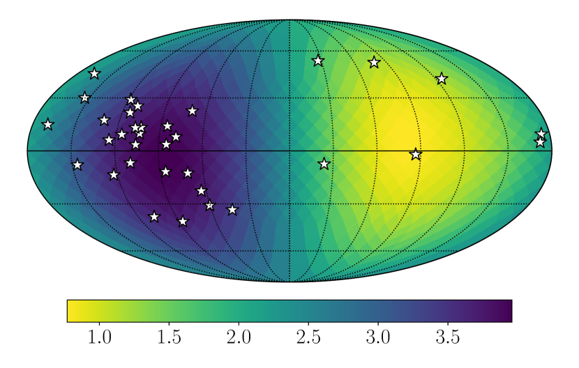
Finally, it is a simple matter to recast the form of the sky map so that we solve (82) for the strain amplitude $h_{0}$ of a monochromatic binary, cf. (44), that would produce a particular value of the signal-to-noise ratio $\rho$:

$$h_{0}(\hat{n})={\rho}\sqrt{\frac{S_{\rm eff}(f_{0},\hat{k})}{T_{\rm obs}}}\,.$$ (83)

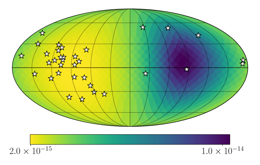
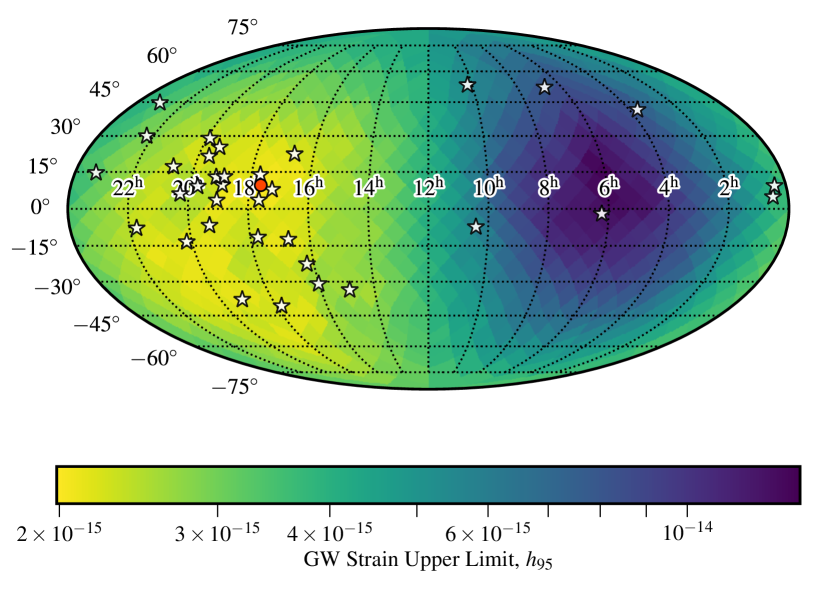
A sky map of $h_{0}(\hat{n})$ is shown in panel (a) of Figure 11 for $\rho=2$ using the NANOGrav 11-year data. For comparison, panel (b) shows the actual 95% confidence-level upper limit map taken from the NANOGrav 11-year single-source paper Aggarwal et al. (2018).

Figure 11: Panel (a): Sensitivity sky map for the strain amplitude of a monochromatic continuous-wave source, calculated using the NANOGrav 11-year data Arzoumanian et al. (2018). For this plot, we have taken $f_{0}=8\leavevmode\nobreak\ {\rm nHz}$ and $\rho=2$. Panel (b): For comparison, a 95% confidence-level upper limit sky map taken from the NANOGrav 11-year single-source paper Aggarwal et al. (2018).

IV.2 Single-pulsar characteristic strain noise curves

For an individual pulsar, we will use the characteristic strain

$$h_{c,I}(f)\equiv\sqrt{fS_{I}(f)}\,,\quad S_{I}(f)\equiv\frac{1}{{\cal N}_{I}^{-1}(f){\cal R}(f)}\,,$$ (84)

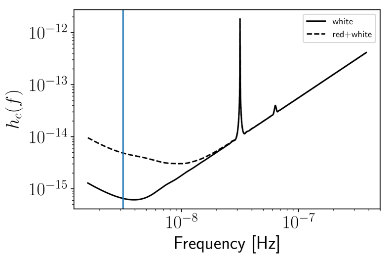
to characterize its polarization and sky-averaged sensitivity; see (74). Plots of single-pulsar characteristic strain-noise sensitivity curves for the simple quadratic spin-down model described in Section II.1 and for both white and red+white noise are shown in Figure 12.

Figure 12: Single-pulsar characteristic strain-noise sensitivity curves for the simple quadratic spin-down timing model fit described in the main text and for white noise (solid curve) and red+white noise (dashed curve). The vertical blue line corresponds to a frequency of $1/T$.

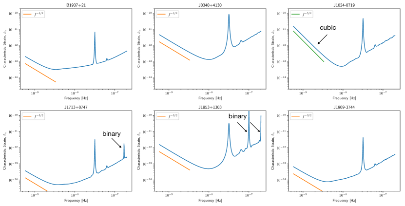
More realistic single-pulsar strain-noise sensitivity curves can be constructed using a subset of the NANOGrav 11-year pulsars (Figure 13) Arzoumanian et al. (2018).

Figure 13: Single-pulsar characteristic strain-noise sensitivity curves for a subset of NANOGrav 11-year pulsars. The $\sim\!f^{-5/2}$ behavior for PSR J1024-0719 is evidence of a fit to a cubic spin-down model for the pulsar spin frequency. The cubic term in the fit is needed due to an acceleration of the pulsar, evident in the TOAs from its unusually-long binary period Arzoumanian et al. (2018); Kaplan et al. (2016). The additional spikes seen for J1713+0747 and J1853+1303 show that the pulsar is in a binary system; the second binary spike for J1853+1303 is the second harmonic of the binary orbital frequency.

These pulsars have noise contributions specified by the parameters EQUAD, ECORR, and EFAC Arzoumanian et al. (2018); Lam et al. (2017); Arzoumanian et al. (2014), which are denoted by $Q$, $J_{ij}$, and $F$ in the following expression for the noise covariance matrix:

$$C_{n,ij}=F^{2}\,[\sigma_{i}^{2}\,\delta_{ij}+Q^{2}\delta_{ij}]+J_{ij}\,.$$ (85)

Here $\sigma_{i}^{2}$ are individual TOA errors, which are associated with the finite-signal-to-noise ratio determination of the pulse arrival times (obtained by correlating the observed pulses with a pulse template). EQUAD are white noise contributions to the covariance matrix that add in quadrature with the TOA errors. EFAC is an overall scale factor that can be used to adjust the overall uncertainty if necessary. ECORR are noise contributions that are correlated within an observing epoch, but not from epoch to epoch. Hence the ECORR contributions to the covariance matrix are block diagonal. Red noise, modeled as a power law, was added for those pulsars that show significant detections in the NANOGrav 11-year data set Arzoumanian et al. (2018). In Figure 13, B1937+21, J1713+0747 and J1909-3744 have injections of red noise. This can be distinguished by the “flatter” appearance of the sensitivity curves around the minimum, as compared to the other pulsars. For a detailed list of noise parameters, and to see which pulsars have significant detections of red noise, consult Table 2 in Arzoumanian et al. (2018).

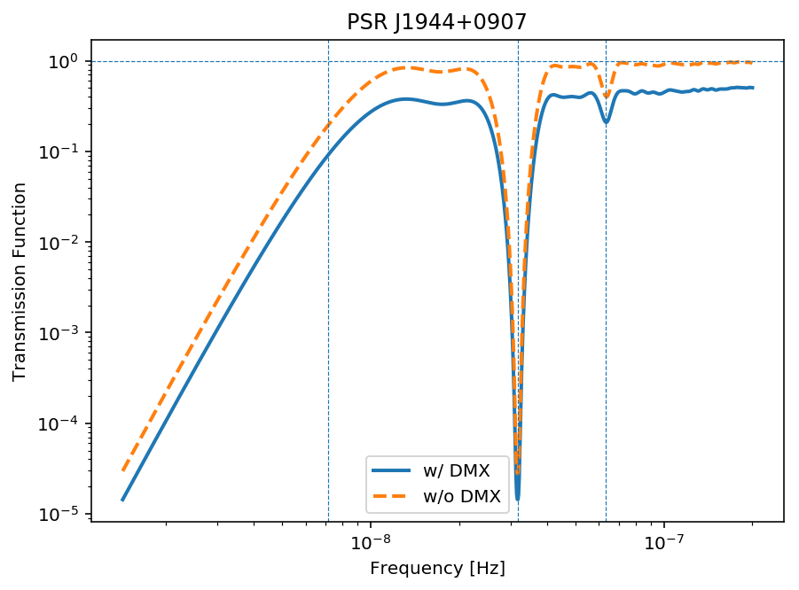
The NANOGrav 11-year pulsars also have more complicated timing model fits than the simple quadratic spin-down model described in Section II.1. In Figure 13, one can see that pulsar J1024-0719 is fit to a cubic spin-down model, leading to a steeper frequency-dependence ($\sim\!f^{-5/2}$) at low frequencies. One also sees that J1713+0747 and J1853+1303 are in binary systems: there are additional spikes at the binary orbital frequency and twice the binary orbital frequency for J1853+1303. Finally, these pulsars have timing models that also include fits to a piecewise, time-dependent dispersion measure fluctuation (DMX), which is associated with perturbations of the dispersion of the radio pulses as they propagate through the interstellar medium from the pulsar to a radio receiver on Earth. (The lower-frequency components of a pulse are delayed more than the higher-frequency components.) Fitting to DMX in the timing model leads to broadband absorption of power relative to a timing model that doesn’t fit for DMX. Figure 14 shows plots of the transmission function for NANOGrav pulsar J1944+0907, with and without DMX included in the timing model.

Figure 14: Plots of transmission functions showing the effect of including time-dependent dispersion measure (DMX) into the timing model fit. Including DMX in the timing model leads to broadband absorption of power (solid blue curve) relative to that for a timing model without DMX.

IV.3 Optimal cross-correlation statistic for a stochastic GW background

The derivation of the optimal cross-correlation statistic for a stochastic GW background is similar to that presented above for a single deterministic GW, expect that we work with data from pairs of pulsars. Starting with a single distinct pair, labeled by $I$ and $J$, we define

$$\hat{\mathcal{S}}_{IJ}\equiv r_{I}^{T}Q\,r_{J}\,,$$ (86)

where $r_{I}$ and $r_{J}$ are the TMM residuals for pulsars $I$ and $J$ (assuming that we have already fit for all deterministic GW sources), and $Q$ is an $m_{I}\times m_{J}$ matrix, where $m_{I}\equiv N_{I}-N_{{\rm par},I}$, etc. As before, we determine the filter function $Q$ by maximizing the signal-to-noise ratio of $\hat{\mathcal{S}}_{IJ}$. Similar derivations appear in the literature Allen and Romano (1999); Anholm et al. (2009); Ellis et al. (2012); Chamberlin et al. (2015); Vigeland et al. (2017). The final result for the optimal filter is

$$Q\propto\,\Sigma_{I}^{-1}\Sigma_{IJ}\Sigma_{J}^{-1}\,,$$ (87)

where

$$\Sigma_{I}\equiv G_{I}^{T}(C_{n,I}+C_{h})G_{I}\,,$$ (88)

$$\Sigma_{IJ}\equiv\chi_{IJ}\,G_{I}^{T}C_{h}G_{J}\,.$$

The expected squared signal-to-noise ratio for this optimal choice of $Q$ is then

$$\rho_{IJ}^{2}={\rm Tr}\left[\Sigma_{JI}\,\Sigma_{I}^{-1}\Sigma_{IJ}\Sigma_{J}^{-1}\right]\,.$$ (89)

The above calculation assumes that we are in the weak-signal limit where the cross-correlation terms are assumed to be negligible compared to auto-correlation terms (i.e., we assume that the GW signal power is much less than that for the intrinsic pulsar and measurement noise).

We can then combine the signal-to-noise ratios for each distinct pair in quadrature since, in the weak-signal limit, there is negligible correlation between these estimators:

$$\rho^{2}\simeq\sum_{I}\sum_{J>I}\rho_{IJ}^{2}.$$ (90)

As we saw for deterministic GWs, it is useful to write the above expression for the expected squared signal-to-noise ratio in the frequency domain. Proceeding as we did there, we find

$$\rho^{2}\simeq\sum_{I}\sum_{J>I}2T_{IJ}\chi_{IJ}^{2}\\ \times\int_{0}^{f_{\rm Nyq}}{\rm d}f\>S^{2}_{h}(f)\mathcal{R}^{2}(f)\mathcal{N}^{-1}_{I}(f)\mathcal{N}^{-1}_{J}(f)\,,$$ (91)

where $P_{h}(f)=\mathcal{R}(f)S_{h}(f)$, and where $\mathcal{N}_{I}^{-1}(f)$ is defined by (20). This suggests defining the following effective strain-noise power spectral density for the whole PTA:

$$S_{\rm eff}(f)=\left(\sum_{I}\sum_{J>I}\frac{T_{IJ}}{T_{\rm obs}}\frac{\chi^{2}_{IJ}}{S_{I}(f)S_{J}(f)}\right)^{-1/2}\,,$$ (92)

which includes contributions from the Hellings and Downs factors $\chi_{IJ}$ and the individual pulsar strain-noise power spectral densities $S_{I}(f)\equiv 1/(\mathcal{N}^{-1}_{I}(f)\mathcal{R}(f))$. Note that $S_{\rm eff}(f)$ has dimensions of strain²/Hz, and that

$$\rho^{2}\simeq 2T_{\rm obs}\int_{0}^{f_{\rm Nyq}}{\rm d}f\>\frac{S_{h}^{2}(f)}{S_{\rm eff}^{2}(f)}$$ (93)

in terms of $S_{\rm eff}(f)$.

Figure 15: Comparison of stochastic sensitivity curves (effective characteristic strain noise) for the NANOGrav 11-year PTA. All the curves include realistic pulsar noise characteristics and individual timing model fits. The blue curve includes a contribution to the auto-power spectra, produced by a GWB at the level of $A_{\rm gwb}=1\times 10^{-16}$. The dashed-orange curve shows the sensitivity without including the GWB, and the green curve shows what happens if you also ignore the red noise contributions to the noise covariance matrices.

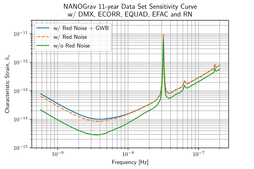
A plot comparing dimensionless charateristic strain curves $h_{c}(f)\equiv\sqrt{fS_{\rm eff}(f)}$ for stochastic GW backgrounds for the NANOGrav 11-year pulsars is given in Figure 15. The three curves show the effect of including a contribution from the GWB to the auto-power spectra of all the pulsars (blue versus dashed-orange curves) and the false improvement in sensitivity that arises if one fails to include the red-noise component of the individual pulsar noise covariance matrices (green versus dashed-orange curves). Typical PTA sensitivity curves that one sees in the literature incorrectly ignore this red noise component.

IV.3.1 Comparing stochastic and deterministic sensitivity curves

Although one uses different statistics to search for deterministic and stochastic GW signals, it is interesting to compare the sensitivity curves for these two different cases. Figure 16 shows plots of the deterministic and stochastic sensitivity curves for the NANOGrav 11-year pulsars (taken from Figure 9 and Figure 15, dashed-orange curve). Note that the sensitivity curve for a single deterministic source is lower than that for a stochastic background, since the Hellings and Downs factors $\chi_{IJ}$ in (92) reduce the effective number of pulsar pairs that contribute to the stochastic analysis.

Figure 16: Comparison of the sensitivity curves for the NANOGrav 11-year pulsars to a single deterministic GW signal and a stochastic GW background; see also Figures 9 and 15. The two curves differ by a factor of $\sim 2.6$.

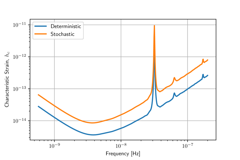
To demonstrate this explicitly, compare equations (73) and (92) for $S_{\rm eff}(f)$ assuming that all the pulsars have the same noise characteristics and timing model fits (i.e., $S_{I}(f)\equiv S(f)$ for all $I$), and that all the pulsars are observed for the full observation time (i.e., $T_{I}\equiv T_{IJ}\equiv T_{\rm obs})$. Then

$$S_{\rm eff}^{\rm det}(f)=\frac{5}{4N_{\rm p}}\,S(f)\,,$$ (94)

$$S_{\rm eff}^{\rm stoch}(f)=\left(\sum_{I}\sum_{J>I}\chi_{IJ}^{2}\right)^{-1/2}S(f)\,,$$ (95)

where $N_{\rm p}$ is the number of pulsars. Since the maximum value of $\chi_{IJ}$ for any pair of pulsars is $1/2$, we have

$$\sum_{I}\sum_{J>I}\chi_{IJ}^{2}\leq\frac{N_{\rm p}(N_{\rm p}-1)}{2}\frac{1}{4}\,,\quad$$ (96)

which implies

$$\left(\sum_{I}\sum_{J>I}\chi_{IJ}^{2}\right)^{-1/2}>\frac{2\sqrt{2}}{N_{\rm p}}\,,$$ (97)

Thus,

$$S_{\rm eff}^{\rm stoch}(f)>\frac{2\sqrt{2}}{N_{\rm p}}\,S(f)\ \Rightarrow\ S_{\rm eff}^{\rm stoch}(f)>S_{\rm eff}^{\rm det}(f)\,.$$ (98)

Although we have compared the full sensitivity curves $S_{\rm eff}(f)$ for deterministic and stochatic GW sources, we note that the corresponding signal-to-noise ratio for a monochromatic deterministic source uses only the value of the sensitivity curve at a single frequency $f=f_{0}$ (see (76)); while that for a stochastic source involves an integral of $S_{\rm eff}(f)$ over all $f$ (see (93) and the discussion in Section IV.3.3).

IV.3.2 Pairwise stochastic sensitivity curves

As a by-product of the stochastic sensitivity curve analysis, we obtain pairwise stochastic sensitivity cuves

$$h_{c,IJ}\equiv\sqrt{fS_{IJ}(f)}\,,\quad S_{IJ}(f)\equiv\sqrt{\frac{T_{\rm obs}}{T_{IJ}}}\frac{\sqrt{S_{I}(f)S_{J}(f)}}{|\chi_{IJ}|}\,,$$ (99)

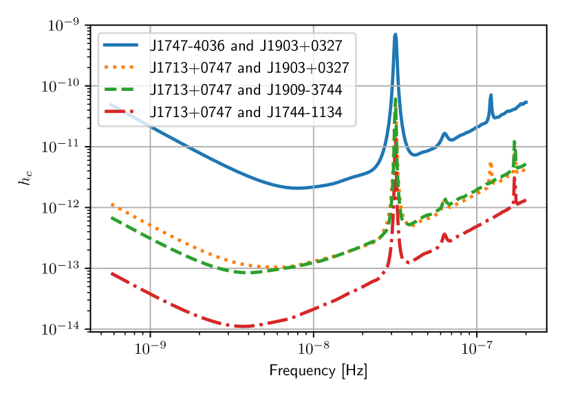
by simply restricting ourselves to a single term in the sum (92). Plots of such curves are useful as a diagnostic for comparing the contribution of different pulsar pairs to the stochastic optimal statistic signal-to-noise ratio. Figure 17 shows pairwise sensitivity curves for a subset of the NANOGrav 11-year pulsars, comparing pairwise correlations of some of the most and least sensitive NANOGrav pulsars.

Figure 17: Pairwise stochastic sensitivity curves (effective characteristic strain noise) for a subset of NANOGrav 11-year pulsar pairs. Since pulsars J1747-4036 and J1903+0327 are two of the least-sensitive pulsars in the NANOGrav 11-year data set, their pairwise sensitivity curve is worse (that is, higher) than the other pairs shown here. The sensitivity curve for J1713+0747 and J1903+0327 is significantly better, since J1713+0747 is the most sensitive pulsar in the data set; while that for J1713+0747 and J1744-1134 is the best, since both of these pulsars are individually very sensitive and their Hellings-Downs coefficient is $\chi_{IJ}=0.3304$. Pulsars J1713+0747 and J1909-3744 are also both individually very sensitive, but since their Hellings-Downs coefficient is only $\chi_{IJ}=0.0058$, their pairwise sensitivity curve is an order of magnitude worse than that for J1713+0747 and J1744-1134.

IV.3.3 Power-law integrated sensitivity curves

For stochastic backgrounds that have a power-law spectrum, cf. (59), it is possible to construct a sensitivity curve that takes into account the improvement in sensitivity that comes from integrating over frequency Thrane and Romano (2013). Given a range of power-law indices, one determines the amplitude of each power-law background that yields a prescribed value of the optimal statistic signal-to-noise ratio $\rho$ (e.g., $\rho=1$). The envelope of these power-law backgrounds defines the power-law-integrated sensitivity curve for the PTA. Figure 18 shows the $\rho=1$ power-law integrated sensitivity curve for the NANOGrav 11-year data set using the dashed-orange characteristic strain-noise curve from Figure 15.

Figure 18: Power-law-integrated sensitivity curve for the NANOGrav 11-year data set. Each of the straight grey lines represents a power-law GWB detectable with an optimal-statistic signal-to-noise ratio $\rho=1$ for the plotted spectral index. The envelope of these lines (i.e., the maximum value of all the power-law backgrounds at a given frequency) defines the power-law-integrated sensitivity curve for the PTA.

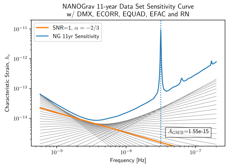
V Discussion

We have presented a method for constructing realistic detection sensitivity curves for pulsar timing arrays, valid for both deterministic and stochastic GW signals. We can include different noise characteristics and the effect of fitting to a timing model via an inverse-noise-weighted transmission function ${\cal N}_{I}^{-1}(f)\approx{\cal T}_{I}(f)/{P(f)}$. Single-pulsar sensitivity curves are then calculated from the strain-noise power spectral density $S_{I}(f)\equiv 1/({\cal N}^{-1}_{I}(f){\cal R}(f))$, where ${\cal R}(f)$ is the polarization and sky-averaged timing residual response of a pulsar to a passing GW. Detection sensitivity curves for multiple pulsars (i.e., a PTA) are similary constructed from an effective strain-noise power spectral density $S_{\rm eff}(f)$, which is a combination of single-pulsar strain-noise power spectral densities $S_{I}(f)$, cf. (73), (78), (92), appropriate for the GW source that one is interested in detecting.

The sensitivity curves that we have calculated can be used to assess the detectability of different GW signals by exisiting or planned PTAs. The computational cost of producing these sensitivity curves is minimal; they can be calculated much faster than doing Monte Carlo simulations using injected signals. By properly incorporating realistic noise properties and the effect of timing model fits into the sensitivity curves, we can produce detectability estimates that agree quite well with the more-computationally-involved predictions.

Appendix A Casting the Blandford et al. analysis Blandford et al. (1984) in more modern notation

When using pulsar timing data to search for GWs, one needs to take into account the effects of fitting to a deterministic timing model when doing any type of additional signal analysis. Following Blandford et al. (1984), we define the residuals $R\left(t\right)$ as the difference between the observed arrival times of the pulses and the expected arrival times as determined by our best guesses to the parameters. These residuals are fit to an expression linear in the corrections to the unknown parameters, $\alpha_{a}$. (Noise terms are added later in their analysis.) We start in the notation of Blandford et al. (1984), and then translate to expressions in terms of modern PTA GW analyses:

$$R\left(t\right)=\sum_{a=1}^{N_{\rm par}}\alpha_{a}\psi_{a}\left(t\right)\,.$$ (100)

We will define $R_{i}\equiv R\left(t_{i}\right)$, which is a vector of length $N$, and $\psi_{ia}\equiv\psi_{a}\left(t_{i}\right)$, which is a 2-dimensional matrix with dimensions $N\times N_{{\rm par}}$. (Note we have reversed the order of the indices on $\psi_{ia}$ from that in Blandford et al. (1984), to be consistent with later work.) In more modern PTA data analysis papers, like van Haasteren and Levin (2013) or Ellis et al. (2013); Chamberlin et al. (2015), this matrix is referred to as the design matrix of the timing model (our $M_{ia}$.) The above expression for the residuals can be transformed into an orthonormal basis

$$R_{i}=\sum_{a=1}^{N_{\rm par}}\alpha_{a}^{\prime}\psi_{ia}^{\prime},\qquad\psi_{ia}^{\prime}\equiv\sum_{b=1}^{N_{\rm par}}\psi_{ib}L_{ba}\,,$$ (101)

where

$$\sum_{i=1}^{N}\psi_{ai}^{\prime T}\psi_{ib}^{\prime}=\delta_{ab}\,.$$ (102)

Using these definitions we calculate a relation that will be useful in the next section. To simplify the notation a bit we will use the Einstein convention of summing over repeated indices without including summation symbols, using matrix transposes where necessary. Thus, for example, the orthonormality conditions can be written as

$$\delta_{ab}=\psi_{ai}^{\prime T}\psi_{ib}^{\prime}=L_{ac}^{T}\psi_{ci}^{T}\psi_{id}L_{db}\,.$$ (103)

Since a change of basis change is invertible, we can act with the inverse transformation matrices:

$$L^{-T}_{ea}\delta_{ab}L^{-1}_{bf} =L_{ea}^{-T}L_{ac}^{T}\psi_{ci}^{T}\psi_{id}L_{db}L_{bf}^{-1}\,,$$ (104)

$$L^{-T}_{ea}L_{af}^{-1} =\psi_{ei}^{T}\psi_{if}\,,$$

where $L^{-T}$ denotes the inverse of the transpose matrix $L^{T}$, which is the same as the transpose of the inverse matrix $L^{-1}$. Finally, using the well-known identity for the inverse of a product of two matrices:

$$\left(L_{ea}^{-T}L_{af}^{-1}\right)^{-1}=\left(\psi_{ei}^{T}\psi_{if}\right)^{-1}\ \Rightarrow\ L_{fa}L_{ae}^{T}=\left(\psi_{ei}^{T}\psi_{if}\right)^{-1}\,.$$ (105)

A.1 Least-squares regression

One finds the best fit to a timing model by minimizing a $\chi^{2}$ function, which we will define below. In Blandford et al. (1984) an ordinary least squares (OLS) minimization is used. In subsequent PTA papers a weighted-least-squares (WLS) regression is used, where each residual is weighted by the inverse of the TOA error, $W_{i}\equiv 1/\sigma_{i}$. In the most modern work a generalized least squares (GLS) regression is used where the noise covariance matrix, $N_{ij}$, is used, encoding covariances between all residuals:

$$\chi^{2}\equiv\left(R_{i}-\alpha_{a}^{\prime}\psi_{ai}^{\prime T}\right)N_{ij}^{-1}\left(R_{j}-\psi_{jb}^{\prime}\alpha_{b}^{\prime}\right)\,.$$ (106)

Here we solve the GLS minimization problem, restricting to simpler scenarios if needed—i.e., $N^{-1}_{ij}=\sigma_{i}^{-2}\,\delta_{ij}$ for the case of WLS, and $N^{-1}_{ij}=\delta_{ij}$ for OLS (as noise is not taken into account during the OLS fit). We minimize the expression for $\chi^{2}$ above by finding the root(s) of the derivative with respect to the parameters:

$$0 =\frac{\partial\chi^{2}}{\partial\alpha_{a}^{\prime}}$$ (107)

$$=-\psi_{ai}^{\prime T}N_{ij}^{-1}R_{j}+\psi_{ai}^{\prime T}N_{ij}^{-1}\psi_{jb}^{\prime}\alpha_{b}^{\prime}+({\rm transpose})\,.$$

Solving for $\alpha_{b}^{\prime}$ gives

$$\alpha_{b}^{\prime}=\left(\psi_{ai}^{\prime T}N_{ij}^{-1}\psi_{jb}^{\prime}\right)^{-1}\psi_{ak}^{\prime T}N_{kl}^{-1}R_{l}.$$ (108)

In Blandford et al. (1984), they consider OLS fitting. There the noise is taken into account after the fit, but its existence is implicit throughout. For instance the difference between the LHS and RHS side of their Equation (2.9) would be zero if there was no noise. Setting $N_{ij}=\delta_{ij}$ gives

$$\alpha_{b}^{\prime}=\left(\psi_{ai}^{\prime T}\psi_{ib}^{\prime}\right)^{-1}\psi_{aj}^{\prime T}R_{j}=\delta_{ab}^{-1}\,\psi_{aj}^{\prime T}R_{j}\\ =\psi_{bi}^{\prime T}R_{i}\,.$$ (109)

This is the result that Blandford et al. (1984) reports for the best fit. For WLS fitting, we have

$$\alpha_{b}^{\prime}=\left(\psi_{ai}^{\prime T}W_{ij}^{2}\psi_{jb}^{\prime}\right)^{-1}\psi_{ak}^{\prime T}W_{kl}^{2}R_{l}\,,$$ (110)

where $W^{2}_{ij}\equiv\sigma_{i}^{-2}\,\delta_{ij}$.

A.2 Transmission function for ordinary least-squares regression

The transmission function is defined by Blandford et al. (1984) as the transfer function relating the power in the pre-fit residuals $R_{i}$ to that in the post-fit residuals

$$R^{\rm post}_{i}\equiv R_{i}-\psi^{\prime}_{ia}\alpha_{a}^{\prime}\,,$$ (111)

where $\alpha_{a}^{\prime}$ are the best-fit values to the parameter deviations, determined by the $\chi^{2}$ minimization procedure discussed above. For the case of OLS fitting, which Blandford et al. (1984) consider, $\alpha_{a}^{\prime}$ is given by (109), implying

$$R^{\rm post}_{i}\equiv R_{i}-\psi^{\prime}_{ia}\psi^{\prime T}_{aj}R_{j}=(\delta_{ij}-\psi^{\prime}_{ia}\psi^{\prime T}_{aj})R_{j}\,.$$ (112)

The variance in the post-fit residual is then

$$\sigma^{2}_{\rm post} \equiv\frac{1}{N}\langle R^{\rm post}{}^{T}R^{\rm post}\rangle$$ (113)

$$=\frac{1}{N}\langle R_{j}R_{k}\rangle\left(\delta_{ji}-\psi^{\prime}_{ja}\psi^{\prime T}_{ai}\right)\left(\delta_{ik}-\psi^{\prime}_{ib}\psi^{\prime T}_{bk}\right)$$

$$=\frac{1}{N}\langle R_{j}R_{k}\rangle\left(\delta_{jk}-\psi^{\prime}_{ja}\psi^{\prime T}_{ak}-\psi^{\prime}_{jb}\psi^{\prime T}_{bk}+\psi^{\prime}_{ja}\psi^{\prime T}_{ai}\psi^{\prime}_{ib}\psi^{\prime T}_{bk}\right)$$

$$=\frac{1}{N}\langle R_{j}R_{k}\rangle\left(\delta_{jk}-\psi^{\prime}_{ja}\psi^{\prime T}_{ak}\right)\,,$$

where we used orthogonality of the $\psi^{\prime}_{ja}$ to get the last line. Since the covariance matrix $\langle R_{i}R_{j}\rangle$ is related to its power spectral density $P(f)$ via

$$\langle R_{i}R_{j}\rangle=\int_{0}^{\infty}{\rm d}f\>P(f)\,e^{i2\pi f(t_{i}-t_{j})}\,,$$ (114)

it follows that

$$\sigma^{2}_{\rm post}=\int_{0}^{\infty}{\rm d}f\>{\cal T}(f)P(f)\,,$$ (115)

where

$${\cal T}\left(f\right) \equiv 1-\frac{1}{N}\psi_{ia}^{\prime}\psi_{aj}^{\prime T}e^{i2\pi f\left(t_{i}-t_{j}\right)}$$ (116)

$$=1-\frac{1}{N}\tilde{\psi}_{a}^{\prime}\left(f\right)\left(\tilde{\psi}_{a}^{\prime}\left(f\right)\right)^{\dagger}$$

with $\tilde{\psi}_{a}^{\prime}$ the Fourier transforms of the basis functions:

$$\tilde{\psi}_{a}^{\prime}\left(f\right)={\psi}_{ia}^{\prime}e^{i2\pi ft_{i}}.$$ (117)

Making this substitution and transforming $\psi_{ia}^{\prime}$ back to the original basis, we find

$${\cal T}\left(f\right) =1-\frac{1}{N}\psi_{ib}L_{ba}L_{ac}^{T}\psi_{cj}^{T}e^{i2\pi f\left(t_{i}-t_{j}\right)}$$ (118)

$$=1-\frac{1}{N}\psi_{ib}\left(\psi_{ck}^{T}\psi_{kb}\right)^{-1}\psi_{cj}^{T}e^{i2\pi f\left(t_{i}-t_{j}\right)}$$

$$=\frac{1}{N}\left(\delta_{ij}-\psi_{ib}\left(\psi_{ck}^{T}\psi_{kb}\right)^{-1}\psi_{cj}^{T}\right)e^{i2\pi f\left(t_{i}-t_{j}\right)}\,,$$

which is an expression for transmission function in terms of the original design matrix $\psi_{ia}$.

A.3 Transmission function for generalized least-squares regression

For the case of GLS fitting, the best-fit values for the timing parameter deviations are given by (108), for which the post-fit residuals are given by

$$R_{i}^{\rm post} =R_{i}-\psi^{\prime}_{ia}\left(\psi_{bj}^{\prime T}N_{jk}^{-1}\psi_{ka}^{\prime}\right)^{-1}\psi_{bm}^{\prime T}N_{mj}^{-1}R_{j}$$ (119)

$$=\left(\delta_{ij}-\psi^{\prime}_{ia}\left(\psi_{bk}^{\prime T}N_{kl}^{-1}\psi_{la}^{\prime}\right)^{-1}\psi_{bm}^{\prime T}N_{mj}^{-1}\right)R_{j}\,.$$

We can write this in terms of the original basis as

$$R_{i}^{\rm post} =\left(\delta_{ij}-\psi_{ic}L_{ca}\left(L_{be}^{T}\psi_{ek}^{T}N_{kl}^{-1}\psi_{ld}L_{da}\right)^{-1}L_{bf}^{T}\psi_{fm}^{T}N_{mj}^{-1}\right)R_{j}$$ (120)

$$=\left(\delta_{ij}-\psi_{ic}L_{ca}L_{ad}^{-1}\left(\psi_{ek}^{T}N_{kl}^{-1}\psi_{ld}\right)^{-1}L_{eb}^{-T}L_{bf}^{T}\psi_{fm}^{T}N_{mj}^{-1}\right)R_{j}$$

$$=\left(\delta_{ij}-\psi_{id}\left(\psi_{ek}^{T}N_{kl}^{-1}\psi_{ld}\right)^{-1}\psi_{em}^{T}N_{mj}^{-1}\right)R_{j}\,,$$

which has exactly the same form as (119) with $\psi^{\prime}_{ia}$ replaced by $\psi_{ia}$. The variance of the post-fit residuals is thus

$$\sigma^{2}_{\rm post} \equiv\frac{1}{N}\langle R^{\rm post}{}^{T}R^{\rm post}\rangle$$ (121)

$$=\frac{1}{N}\left(\delta_{ij}-\psi_{ia}\left(\psi_{bl}^{T}N_{lm}^{-1}\psi_{ma}\right)^{-1}\psi_{bn}^{T}N_{nj}^{-1}\right)\langle R_{j}R_{k}\rangle\left(\delta_{ki}-N^{-1}_{kq}\psi_{qc}\left(\psi_{dr}^{T}N_{rs}^{-1}\psi_{sc}\right)^{-1}\psi_{di}^{T}\right)\,.$$

Since $\langle R_{i}R_{j}\rangle\equiv N_{jk}$ for GLS fitting, we get

$$\sigma^{2}_{\rm post} =\frac{1}{N}\left(N_{ik}-\psi_{ia}\left(\psi_{bl}^{T}N_{lm}^{-1}\psi_{ma}\right)^{-1}\psi_{bk}^{T}\right)\left(\delta_{ki}-N^{-1}_{kq}\psi_{qc}\left(\psi_{dr}^{T}N_{rs}^{-1}\psi_{sc}\right)^{-1}\psi_{di}^{T}\right)$$ (122)

$$=\frac{1}{N}\left(N_{ik}\delta_{ki}-\psi_{ia}\left(\psi_{bl}^{T}N_{lm}^{-1}\psi_{ma}\right)^{-1}\psi_{bi}^{T}-\psi_{ic}\left(\psi_{dr}^{T}N_{rs}^{-1}\psi_{sc}\right)^{-1}\psi_{di}^{T}\right.$$

$$\left.\qquad\qquad\qquad\qquad\qquad+\psi_{ia}\left(\psi_{bl}^{T}N_{lm}^{-1}\psi_{ma}\right)^{-1}\psi_{bk}^{T}N_{kq}^{-1}\psi_{qc}\left(\psi_{dr}^{T}N_{rs}^{-1}\psi_{sc}\right)^{-1}\psi_{di}^{T}\right)$$

$$=\frac{1}{N}\left(N_{ik}\delta_{ki}-\psi_{ia}\left(\psi_{bl}^{T}N_{lm}^{-1}\psi_{ma}\right)^{-1}\psi_{bi}^{T}\right)$$

$$=\frac{1}{N}\left(\delta_{ij}-\psi_{ia}\left(\psi_{bl}^{T}N_{lm}^{-1}\psi_{ma}\right)^{-1}\psi_{bk}^{T}N^{-1}_{kj}\right)N_{ij}\,,$$

where we used the symmetry of $N_{ij}$ throughout. Finally, using (114) for $N_{ij}$, we recover (115) with

$${\cal T}\left(f\right)={\cal T}_{R}\left(f\right)\equiv\frac{1}{N}\left(\delta_{ij}-\psi_{ia}\left(\psi_{bl}^{T}N_{lm}^{-1}\psi_{ma}\right)^{-1}\psi_{bk}^{T}N^{-1}_{kj}\right)\,e^{i2\pi f\left(t_{i}-t_{j}\right)}\,.$$ (123)

We thus obtain the same $R$-matrix-dependent transmission function ${\cal T}_{R}(f)$ found in (15), with the $R$-matrix given by the expression in parentheses, $R_{ij}\equiv\delta_{ij}-\psi_{ia}\left(\psi_{bl}^{T}N_{lm}^{-1}\psi_{ma}\right)^{-1}\psi_{bk}^{T}N^{-1}_{kj}$.

References

- Siemens et al. (2013) Xavier Siemens, Justin Ellis, Fredrick Jenet, and Joseph D. Romano, “The stochastic background: scaling laws and time to detection for pulsar timing arrays,” Classical and Quantum Gravity 30, 224015 (2013), arXiv:1305.3196 [astro-ph.IM] .
- Rosado et al. (2015) P. A. Rosado, A. Sesana, and J. Gair, “Expected properties of the first gravitational wave signal detected with pulsar timing arrays,” MNRAS 451, 2417–2433 (2015), arXiv:1503.04803 [astro-ph.HE] .
- Taylor et al. (2016) S. R. Taylor, M. Vallisneri, J. A. Ellis, C. M. F. Mingarelli, T. J. W. Lazio, and R. van Haasteren, “Are We There Yet? Time to Detection of Nanohertz Gravitational Waves Based on Pulsar-timing Array Limits,” ApJ 819, L6 (2016), arXiv:1511.05564 [astro-ph.IM] .
- Kelley et al. (2017) L. Z. Kelley, L. Blecha, L. Hernquist, A. Sesana, and S. R. Taylor, “The gravitational wave background from massive black hole binaries in Illustris: spectral features and time to detection with pulsar timing arrays,” MNRAS 471, 4508–4526 (2017), arXiv:1702.02180 [astro-ph.HE] .
- Sazhin (1978) M. V. Sazhin, “Opportunities for detecting ultralong gravitational waves,” Soviet Ast. 22, 36–38 (1978).
- Detweiler (1979) S. Detweiler, “Pulsar timing measurements and the search for gravitational waves,” Astrophys. J. 234, 1100–1104 (1979).
- Foster and Backer (1990) R. S. Foster and D. C. Backer, “Constructing a pulsar timing array,” Astrophys. J. 361, 300–308 (1990).
- Abbott et al. (2016) B. P. Abbott et al. (LIGO Scientific, Virgo), “Observation of Gravitational Waves from a Binary Black Hole Merger,” Phys. Rev. Lett. 116, 061102 (2016), arXiv:1602.03837 [gr-qc] .
- Abbott et al. (2018) B. P. Abbott et al. (LIGO Scientific, Virgo), “GWTC-1: A Gravitational-Wave Transient Catalog of Compact Binary Mergers Observed by LIGO and Virgo during the First and Second Observing Runs,” (2018), arXiv:1811.12907 [astro-ph.HE] .
- Abbott et al. (2017) B. P. Abbott et al. (LIGO Scientific, Virgo), “GW170817: Observation of Gravitational Waves from a Binary Neutron Star Inspiral,” Phys. Rev. Lett. 119, 161101 (2017), arXiv:1710.05832 [gr-qc] .
- Moore et al. (2015a) C. J. Moore, R. H. Cole, and C. P. L. Berry, “Gravitational-wave sensitivity curves,” Class. Quant. Grav. 32, 015014 (2015a), arXiv:1408.0740 [gr-qc] .
- Robson et al. (2019) Travis Robson, Neil J. Cornish, and Chang Liug, “The construction and use of LISA sensitivity curves,” Class. Quant. Grav. 36, 105011 (2019), arXiv:1803.01944 [astro-ph.HE] .
- Hobbs (2011) George Hobbs, “Pulsars as gravitational wave detectors,” Astrophysics and Space Science Proceedings 21, 229 (2011), arXiv:1006.3969 [astro-ph.SR] .
- Thrane and Romano (2013) Eric Thrane and Joseph D. Romano, “Sensitivity curves for searches for gravitational-wave backgrounds,” Phys. Rev. D88, 124032 (2013), arXiv:1310.5300 [astro-ph.IM] .
- Cordes (1980) J. M. Cordes, “Pulsar timing. II. Analysis of random walk timing noise : application to the Crab pulsar.” ApJ 237, 216–226 (1980).
- Blandford et al. (1984) R. Blandford, R. Narayan, and R. W. Romani, “Arrival-time analysis for a millisecond pulsar.” Journal of Astrophysics and Astronomy 5, 369–388 (1984).
- Cutler et al. (2014) Curt Cutler, Sarah Burke-Spolaor, Michele Vallisneri, Joseph Lazio, and Walid Majid, “The Gravitational-Wave Discovery Space of Pulsar Timing Arrays,” Phys. Rev. D89, 042003 (2014), arXiv:1309.2581 [gr-qc] .
- Madison et al. (2013) D. R. Madison, S. Chatterjee, and J. M. Cordes, “The Benefits of VLBI Astrometry to Pulsar Timing Array Searches for Gravitational Radiation,” Astrophys. J. 777, 104 (2013), arXiv:1210.2469 [astro-ph.HE] .
- Demorest (2007) Paul B. Demorest, Measuring the gravitational wave background using precision pulsar timing, Ph.D. thesis, University of California, Berkeley (2007).
- van Haasteren et al. (2009) Rutger van Haasteren, Yuri Levin, Patrick McDonald, and Tingting Lu, “On measuring the gravitational-wave background using Pulsar Timing Arrays,” Mon. Not. Roy. Astron. Soc. 395, 1005 (2009), arXiv:0809.0791 [astro-ph] .
- Coles et al. (2011) W. Coles, G. Hobbs, D. J. Champion, R. N. Manchester, and J. P. W. Verbiest, “Pulsar timing analysis in the presence of correlated noise,” MNRAS 418, 561–570 (2011), arXiv:1107.5366 [astro-ph.IM] .
- van Haasteren and Levin (2013) Rutger van Haasteren and Yuri Levin, “Understanding and analysing time-correlated stochastic signals in pulsar timing,” Mon. Not. Roy. Astron. Soc. 428, 1147 (2013), arXiv:1202.5932 [astro-ph.IM] .
- Chamberlin et al. (2015) Sydney J. Chamberlin, Jolien D. E. Creighton, Xavier Siemens, Paul Demorest, Justin Ellis, Larry R. Price, and Joseph D. Romano, “Time-domain Implementation of the Optimal Cross-Correlation Statistic for Stochastic Gravitational-Wave Background Searches in Pulsar Timing Data,” Phys. Rev. D91, 044048 (2015), arXiv:1410.8256 [astro-ph.IM] .
- Lee et al. (2012) K. J. Lee, C. G. Bassa, G. H. Janssen, R. Karuppusamy, M. Kramer, R. Smits, and B. W. Stappers, “The optimal schedule for pulsar timing array observations,” MNRAS 423, 2642–2655 (2012), arXiv:1204.4321 [astro-ph.IM] .
- Lee (2016) K. J. Lee, “Prospects of Gravitational Wave Detection Using Pulsar Timing Array for Chinese Future Telescopes,” in Frontiers in Radio Astronomy and FAST Early Sciences Symposium 2015, Astronomical Society of the Pacific Conference Series, Vol. 502, edited by L. Qain and D. Li (2016) p. 19.
- Moore et al. (2015b) Christopher J. Moore, Stephen R. Taylor, and Jonathan R. Gair, “Estimating the sensitivity of pulsar timing arrays,” Class. Quant. Grav. 32, 055004 (2015b), arXiv:1406.5199 [astro-ph.IM] .
- Caballero et al. (2016) R. N. Caballero, K. J. Lee, L. Lentati, G. Desvignes, D. J. Champion, J. P. W. Verbiest, G. H. Janssen, B. W. Stappers, M. Kramer, and P. Lazarus, “The noise properties of 42 millisecond pulsars from the European Pulsar Timing Array and their impact on gravitational-wave searches,” MNRAS 457, 4421–4440 (2016), arXiv:1510.09194 [astro-ph.IM] .
- Ellis et al. (2012) J. A. Ellis, X. Siemens, and J. D. E. Creighton, “Optimal strategies for continuous gravitational wave detection in pulsar timing arrays,” Astrophys. J. 756, 175 (2012), arXiv:1204.4218 [astro-ph.IM] .
- Taylor and Weisberg (1982) J. H. Taylor and J. M. Weisberg, “A new test of general relativity: Gravitational radiation and the binary pulsar PS R 1913+16,” Astrophys. J. 253, 908–920 (1982).
- Romano and Cornish (2017) Joseph D. Romano and Neil J. Cornish, “Detection methods for stochastic gravitational-wave backgrounds: a unified treatment,” Living Rev. Rel. 20, 2 (2017), arXiv:1608.06889 [gr-qc] .
- Detweiler (1979) Steven L. Detweiler, “Pulsar timing measurements and the search for gravitational waves,” Astrophys. J. 234, 1100–1104 (1979).
- Hellings and Downs (1983) R. w. Hellings and G. s. Downs, “UPPER LIMITS ON THE ISOTROPIC GRAVITATIONAL RADIATION BACKGROUND FROM PULSAR TIMING ANALYSIS,” Astrophys. J. 265, L39–L42 (1983).
- Babak et al. (2016) S. Babak, A. Petiteau, A. Sesana, P. Brem, P. A. Rosado, S. R. Taylor, A. Lassus, J. W. T. Hessels, C. G. Bassa, M. Burgay, R. N. Caballero, D. J. Champion, I. Cognard, G. Desvignes, J. R. Gair, L. Guillemot, G. H. Janssen, R. Karuppusamy, M. Kramer, P. Lazarus, K. J. Lee, L. Lentati, K. Liu, C. M. F. Mingarelli, S. Osłowski, D. Perrodin, A. Possenti, M. B. Purver, S. Sanidas, R. Smits, B. Stappers, G. Theureau, C. Tiburzi, R. van Haasteren, A. Vecchio, and J. P. W. Verbiest, “European Pulsar Timing Array limits on continuous gravitational waves from individual supermassive black hole binaries,” MNRAS 455, 1665–1679 (2016), arXiv:1509.02165 .
- Babak and Sesana (2012) S. Babak and A. Sesana, “Resolving multiple supermassive black hole binaries with pulsar timing arrays,” Phys. Rev. D 85, 044034 (2012), arXiv:1112.1075 [astro-ph.CO] .
- Yardley et al. (2010) D. R. B. Yardley, G. B. Hobbs, F. A. Jenet, J. P. W. Verbiest, Z. L. Wen, R. N. Manchester, W. A. Coles, W. van Straten, M. Bailes, N. D. R. Bhat, S. Burke-Spolaor, D. J. Champion, A. W. Hotan, and J. M. Sarkissian, “The sensitivity of the Parkes Pulsar Timing Array to individual sources of gravitational waves,” 407, 669–680 (2010), arXiv:1005.1667 [astro-ph.GA] .
- Arzoumanian et al. (2018) Z. Arzoumanian et al. (NANOGRAV), “The NANOGrav 11-year Data Set: Pulsar-timing Constraints On The Stochastic Gravitational-wave Background,” Astrophys. J. 859, 47 (2018), arXiv:1801.02617 [astro-ph.HE] .
- Aggarwal et al. (2018) K. Aggarwal et al., “The NANOGrav 11-Year Data Set: Limits on Gravitational Waves from Individual Supermassive Black Hole Binaries,” (2018), arXiv:1812.11585 [astro-ph.GA] .
- Kaplan et al. (2016) D. L. Kaplan et al., “PSR J1024-0719: A Millisecond Pulsar in an Unusual Long-Period Orbit,” Astrophys. J. 826, 86 (2016), arXiv:1604.00131 [astro-ph.HE] .
- Lam et al. (2017) M. T. Lam et al., “The NANOGrav Nine-Year Data Set: Excess Noise in Millisecond Pulsar Arrival Times,” Astrophys. J. 834, 35 (2017), arXiv:1610.01731 [astro-ph.HE] .
- Arzoumanian et al. (2014) Z. Arzoumanian et al. (NANOGrav), “Gravitational Waves From Individual Supermassive Black Hole Binaries in Circular Orbits: Limits From the North American Nanohertz Observatory for Gravitational Waves,” Astrophys. J. 794, 141 (2014), arXiv:1404.1267 [astro-ph.GA] .
- Allen and Romano (1999) Bruce Allen and Joseph D. Romano, “Detecting a stochastic background of gravitational radiation: Signal processing strategies and sensitivities,” Physical Review D 59, 102001 (1999), arXiv:gr-qc/9710117 [gr-qc] .
- Anholm et al. (2009) Melissa Anholm, Stefan Ballmer, Jolien D. E. Creighton, Larry R. Price, and Xavier Siemens, “Optimal strategies for gravitational wave stochastic background searches in pulsar timing data,” Phys. Rev. D79, 084030 (2009), arXiv:0809.0701 [gr-qc] .
- Vigeland et al. (2017) S. J. Vigeland, K. P. Islo, J. A. Ellis, and S. R. Taylor, “A noise-marginalized optimal-statistic for pulsar-timing array detection of gravitational waves,” in preparation (2017).
- Ellis et al. (2013) Justin A. Ellis, Xavier Siemens, and Rutger van Haasteren, “An Efficient Approximation to the Likelihood for Gravitational Wave Stochastic Background Detection Using Pulsar Timing Data,” Astrophys. J. 769, 63 (2013), arXiv:1302.1903 [astro-ph.IM] .