Triple singularities of elastic wave propagation in anisotropic media

Abstract

A typical singularity of elastic wave propagation, often termed a shear-wave singularity, takes place when the Christoffel equation has a double root or, equivalently, two out of three slowness or phase-velocity sheets share a common point. We examine triple singularities, corresponding to triple degeneracies of the Christoffel equation, and establish their two notable properties: (i) if multiple triple singularities are present, the phase velocities along all of them are exactly equal, and (ii) a triple singularity maps onto a finite-size planar patch shared by the group-velocity surfaces of the P-, S₁-, and S₂-waves. There are no other known mechanisms that create finite-size planar areas on group-velocity surfaces in homogeneous anisotropic media.

I Introduction

Singularities of seismic wave propagation, defined as the wavefront normal directions along which the Christoffel equation has a double root, constitute a subject of quite an extensive literatureFedorov (1968); Alshits and Lothe (1979a, b); Crampin (1981); Crampin and Yedlin (1981); Musgrave (1981); Alshits et al. (1985); Helbig (1994); Schoenberg and Helbig (1997); Shuvalov (1998); Boulanger and Hayes (1998); Vavryčuk (2001, 2003, 2005a, 2005b); Alshits (2003); Goldin (2013); Grechka (2015, 2017); Ivanov (2019). The interest to singularities can be explained, at least partly, by their ubiquity — they are found in all natural anisotropic elastic solids.

The so-called three-fold or triple singularities, where the Christoffel equation possesses a triple root, on the other hand, are mentioned in a handful of papersAlshits and Lothe (1979a); Musgrave (1981); Alshits et al. (1985); Alshits (2003) only and not well known in both acoustical and geophysical communities. The reason for that, presumably, is the instability of triple singularities with respect to a small arbitrary perturbation of the stiffness tensorAlshits et al. (1985). Because the lack of their stability should not disqualify them from theoretical investigation, we present a study of their features.

II Theory

The classic ChristoffelChristoffel (1877); Fedorov (1968); Musgrave (1970) equation

$$\bm{\Gamma}(\bm{n})\bm{\cdot U}=V^{2}\,\bm{U}\,$$ (1)

describes propagation of plane body waves in homogeneous anisotropic media. Here

$$\bm{\Gamma}(\bm{n})\equiv\bm{n\cdot c\cdot n}\,$$ (2)

is the $3\times 3$ Christoffel tensor or matrix, $\bm{c}$ is the $3\times 3\times 3\times 3$ density-normalized stiffness tensor, $\bm{n}$ is the unit normal to a plane wavefront, $V$ is the phase velocity, and $\bm{U}$ is the unit polarization vector. Mathematically, equation 1 is the standard eigenvalue-eigenvector problem for the $3\,\times\,3$ symmetric, positive-definite matrix $\bm{\Gamma}(\bm{n})$; the eigenvalues of $\bm{\Gamma}(\bm{n})$ are the squared phase velocities $V^{2}>0$ of the three isonormal plane waves, termed the P-, fast shear S₁-, and slow shear S₂-waves; the eigenvectors of $\bm{\Gamma}(\bm{n})$ are the unit polarization vectors $\bm{U}$ of these waves.

Triple singularities are defined as wavefront normal directions $\bm{n}=\bm{n}^{t}$ along which equation 1 has three coinciding eigenvalues,

$$V_{\mathrm{P}}^{2}(\bm{n}^{t})=V_{\mathrm{S1}}^{2}(\bm{n}^{t})=V_{\mathrm{S2}}^{2}(\bm{n}^{t})\equiv V_{t}^{2}\,.$$ (3)

As a consequence of equalities 3, the Christoffel tensor 2 possesses a triplet of arbitrarily oriented, mutually orthogonal eigenvectors $\bm{U}^{\mathrm{P}}(\bm{n}^{t})\perp\bm{U}^{\mathrm{S1}}(\bm{n}^{t})\perp\bm{U}^{\mathrm{S2}}(\bm{n}^{t})$. Therefore, tensor $\bm{\Gamma}(\bm{n}^{t})$ has to be scalarAlshits et al. (1985),

$$\bm{\Gamma}(\bm{n}^{t})=V_{t}^{2}\,\bm{I}\,,$$ (4)

where $\bm{I}$ is the $3\times 3$ identity matrix. Equation 4 implies that certain equality-type constraints have to be imposed on the components of elastic stiffness tensor $\bm{c}$ for mere existence of a triple singularity.

Perhaps the easiest way to determine these constraints is to orient the axis $\bm{x}_{3}$ of a local Cartesian coordinate frame along $\bm{n}^{t}$, making $\bm{n}^{t}=[0,~{}0,~{}1]$, and

$$\bm{\Gamma}(\bm{n}^{t})=\left(\begin{array}[]{c c c}c_{55}&c_{45}&c_{35}\\ c_{45}&c_{44}&c_{34}\\ c_{35}&c_{34}&c_{33}\\ \end{array}\right)\!,$$ (5)

where the Voigt ruleMusgrave (1970); Tsvankin (2001); Grechka (2009) is applied to transition from the four-index notation of the components of fourth-rank stiffness tensor $\bm{c}$ to the two-index notation in matrix 5.

The comparison of equations 4 and 5 reveals the sought equalities for the stiffness components

$$c_{34}=c_{35}=c_{45}=0\,,$$ (6a)

$$c_{33}=c_{44}=c_{55}=V_{t}^{2}$$ (6b)

in the selected local coordinate frame. Equations 6b clearly indicate the instability of triple singularities Alshits et al. (1985) under an arbitrary triclinic perturbation of tensor $\bm{c}$, pointing to a low probability of finding triple singularities in natural homogeneous solids like crystals. Setting these issues (revisited in the Discussion section) aside, triple singularities can be examined as purely theoretical or mathematical objects, just as anisotropic solids without conventional singularities Alshits and Lothe (1979b) have been studied.

Such an investigation of triple singularities begins by recognizing “a wholly arbitrary choice”Musgrave (1981) of unit polarization vector

$$\bm{U}^{t}\equiv\bm{U}(\bm{n}^{t},\,\varphi_{1},\,\varphi_{2})=[\sin\varphi_{1}\cos\varphi_{2},~{}\sin\varphi_{1}\sin\varphi_{2},~{}\cos\varphi_{1}]\,,\quad(0\leq\varphi_{1}\leq\pi,~{}0\leq\varphi_{2}\leq 2\,\pi)\,$$ (7)

as an eigenvector of tensor $\bm{\Gamma}(\bm{n}^{t})$. Next, the general definition of group-velocity vectorFedorov (1968); Musgrave (1970)

$$\bm{g}=\bm{\Gamma}(\bm{U})\bm{\cdot}\frac{\bm{n}}{V}$$ (8)

and, specifically,

$$\bm{g}^{t}\equiv\bm{g}(\bm{n}^{t},\,\varphi_{1},\,\varphi_{2})=\bm{\Gamma}(\bm{U}^{t})\bm{\cdot}\frac{\bm{n}^{t}}{V_{t}}$$ (9)

yields the components of $\bm{g}^{t}$:

$$g_{1}^{t} =\frac{\sin\varphi_{1}}{V_{t}}\,\Big{\{}\cos\varphi_{1}\,\big{[}(c_{13}+c_{55})\,\cos\varphi_{2}+c_{36}\,\sin\varphi_{2}\big{]}+\sin\varphi_{1}\,\big{[}c_{15}\,\cos^{2}\varphi_{2}+(c_{14}+c_{56})\,\cos\varphi_{2}\,\sin\varphi_{2}$$ (10)

$$\hskip 85.35826pt+\,c_{46}\,\sin^{2}\varphi_{2}\,\big{]}\Big{\}},$$

$$g_{2}^{t} =\frac{\sin\varphi_{1}}{V_{t}}\,\Big{\{}\cos\varphi_{1}\,\big{[}(c_{23}+c_{55})\,\sin\varphi_{2}+c_{36}\,\cos\varphi_{2}\big{]}+\sin\varphi_{1}\,\big{[}c_{56}\,\cos^{2}\varphi_{2}+(c_{25}+c_{46})\,\cos\varphi_{2}\,\sin\varphi_{2}$$ (11)

$$\hskip 85.35826pt+\,c_{24}\,\sin^{2}\varphi_{2}\,\big{]}\Big{\}},$$

$$g_{3}^{t} =V_{t}\,$$ (12)

in our local coordinate frame.

Let us note the following.

• Vectors $\bm{g}(\bm{n}^{t},\,\varphi_{1},\,\varphi_{2})$ fill a solid conical object rather than trace the surface of an internal refraction cone, as analogous group-velocity vectors do at conventional (double) singularities.

• The component $g_{3}^{t}$ given by equation 12 is independent of the polarization angles $\varphi_{1}$ and $\varphi_{2}$; therefore, the base $\bm{g}^{Q}$ of the internal refraction cone is a plane with the unit normal $\bm{n}^{t}$.

• The non-quadratic dependencies of the components $g_{1}^{t}$ and $g_{2}^{t}$ on sines and cosines of angles $\varphi_{1}$ and $\varphi_{2}$ in equations 10 and 11 generally result in a quartic rather than elliptic (as for conventional singularities) shape of the base of an internal refraction cone, the feature of triple singularities illustrated in Figure 1 for a triclinic model that has the density-normalized stiffness tensor (in arbitrary units of velocity squared, as well as other stiffness tensors below)

$$\bm{c}=\left(\begin{array}[]{c c c c c c}12&3&0&0.1&0.2&0.3\\ {}\hfil&10&5&0.4&0.5&0.6\\ {}\hfil&{}\hfil&6&0&0&0.4\\ {}\hfil&\mathrm{SYM}&{}\hfil&6&0&0.7\\ {}\hfil&{}\hfil&{}\hfil&{}\hfil&6&0.8\\ {}\hfil&{}\hfil&{}\hfil&{}\hfil&{}\hfil&4\\ \end{array}\right)\!.$$ (13)

Here “SYM” denotes symmetric part of the stiffness matrix.

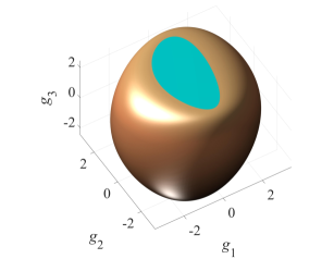
Figure 1: The P-wave group-velocity surface (copper) in triclinic model 13. The planar portion of the surface displayed in cyan is the base $\bm{g}^{Q}$ of the internal refraction cone formed at triple singularity $\bm{n}^{t}=[0,\,0,\,1]$.

It is straightforward to show that finite-size planar patches can be formed on group-velocity surfaces only in conjunction with triple singularities. To see this, consider finite-size regular area of a group-velocity surface. Its flatness implies the zero Gaussian curvature, $\mathcal{K}_{\,g}=\mathcal{K}_{\,g}(\bm{n})=0$, for a range of the wavefront-normal vectors $\bm{n}$. Consequently, Gaussian curvature $\mathcal{K}_{\,p}$ of regular area of the corresponding slowness surface has to be infinite becauseGrechka and Obolentseva (1993); Vavryčuk and Yomogida (1996)

$$\mathcal{K}_{\,p}\,{\mathcal{K}_{\,g}}=\left(\frac{V}{|\bm{g}|}\right)^{\!4},$$ (14)

and the right side of equation 14 has to be finite to satisfy the elastic stability conditions. The equality $\mathcal{K}_{\,p}=\infty$ over a finite area of a slowness surface violates the differentiability of the Christoffel equation 1 written in slownesses and implies that finite-size regular region of a group-velocity surface cannot be planar, leaving singularities as the only remaining option. However, neither conventional conical nor intersection singularities yield flat areas of the group-velocity surfaces; the former, occurring along isolated wavefront-normal directions, map themselves onto elliptical lines of the zero Gaussian curvatureShuvalov and Every (1997) $\mathcal{K}_{\,g}=0$ rather than onto finite-size areas; the latter, shaped as circles in transversely isotropic media, do give rise to the zero Gaussian curvature areas but these areas, either conical or cylindric, are not planar (see an example in section VI).

III The minimax property

The phase velocity $V_{t}$ defined by equations 3 possesses a remarkable propertyAlshits and Lothe (1979a); Alshits (2003)

$$V_{t}=\min\limits_{(\bm{n})}V_{\mathrm{P}}(\bm{n})=\max\limits_{(\bm{n})}V_{\mathrm{S2}}(\bm{n})\,.$$ (15)

In a word, velocity $V_{t}$ in the direction of triple singularity $\bm{n}^{t}$ is equal to both

• the global minimum of the outermost phase-velocity sheet $V_{\mathrm{P}}(\bm{n})$ and

• the global maximum of the innermost phase-velocity sheet $V_{\mathrm{S2}}(\bm{n})$.

This statement is a direct consequence of inequalityAlshits and Lothe (1979b)

$$V_{\mathrm{P}}\!\left(\bm{n}^{a}\right)\geq V_{\mathrm{S2}}\!\left(\bm{n}^{b}\right)~{}\forall~{}\,\bm{n}^{a}~{}\text{and}~{}\bm{n}^{b}\,.$$ (16)

Indeed, in accordance with equations 3, the wavefront normal direction $\bm{n}^{a}=\bm{n}^{b}=\bm{n}^{t}$ is exactly where

$$V_{\mathrm{P}}(\bm{n}^{t})=V_{\mathrm{S2}}(\bm{n}^{t})=V_{t}\,,$$ (17)

turning inequality 16 into equality.

The minimax property 15 leads to another noteworthy corollary,

If an anisotropic solid possesses $N$ distinct triple singularities $\bm{n}^{t_{1}},\,\ldots,\,\bm{n}^{t_{N}}$, the phase velocities along all of them are equal,

$$V\!\left(\bm{n}^{t_{1}}\right)=\ldots=V\!\left(\bm{n}^{t_{N}}\right)=V_{t}\,.$$ (18)

IV The maximum number of triple singularities

To establish the maximum number $N$ of triple singularities in equation 18, we rewrite equation 4 as

$$\bm{\Gamma}(\bm{p}^{t})=\bm{I},$$ (19)

where

$$\bm{p}^{t}=\frac{\bm{n}^{t}}{V_{t}}\,$$ (20)

is the slowness vector in at a triple singularity. Next, we recognize equation 19 as a system of six quadratic equations for three unknown components of vector $\bm{p}^{t}$.

In general, system 19 is incompatible because it contains six equations for only three unknowns. Its incompatibility is consistent though with equality-type constraints 6b on the stiffness coefficients that have to be imposed in the special coordinate frame for the triple singularity directed at $\bm{n}^{t}=[0,\,0,\,1]$. Bearing the necessity of these constraints in mind, we split system 19 into two subsystems, each including three equations for three elements ${\Gamma}_{ij}(\bm{p}^{t})$ of the Christoffel matrix $\bm{\Gamma}(\bm{p}^{t})$. The first subsystem of three polynomial equations

$${\Gamma}_{ij}(\bm{p}^{t})=\left\{\begin{array}[]{rl}0&\!\text{if }\,i\neq j\,,\\ 1&\!\text{if }\,i=j\,,\\ \end{array}\right.$$ (21)

in which $i=j$ for at least one of the equations, could be solved for the three components of $\bm{p}^{t}$; whereas the remaining subsystem,

$${\Gamma}_{i^{\prime}j^{\prime}}(\bm{p}^{t})=\left\{\begin{array}[]{rl}0&\!\text{if }\,i^{\prime}\neq j^{\prime}\,,\\ 1&\!\text{if }\,i^{\prime}=j^{\prime}\,,\\ \end{array}\right.$$ (22)

comprising three equations for three elements ${\Gamma}_{i^{\prime}j^{\prime}}(\bm{p}^{t})$ of matrix $\bm{\Gamma}(\bm{p}^{t})$ with pairs of indexes $(i^{\prime},\,j^{\prime})\neq(i,\,j)$, would provide constraints on stiffnesses $\bm{c}$ analogous to those given by equations 6b.

If three equations 21 are compatible and non-degenerative, the maximum number of their real-valued roots is given by Bézout’s theoremWeisstein (2003) as a product of the degrees of equations, that is, $2\times 2\times 2=8$. We note that real-valued roots of equations 21 always appear in centrally symmetric pairs $\bm{p}^{t}$ and $-\bm{p}^{t}$ because the left sides ${\Gamma}_{ij}(\bm{p}^{t})$ of equations 21 are homogeneous functions of degree 2 of the components of vector $\bm{p}^{t}$; hence, the maximum number $N$ of distinct, non-centrally symmetric triple singularities is equal to

$$N=4\,.$$ (23)

In general, there is no guarantee that triplets of equations 22, which have to be satisfied for all real-valued roots $\bm{p}^{t_{k}}$ of subsystem 21, yield a compatible set of constraints on the stiffness coefficients $\bm{c}$ similar to equations 6b. If subsystem 22 happens to be self-contradictory for some roots $\bm{p}^{t_{k}}$, the directions of those vectors $\bm{p}^{t_{k}}$ would not obey the criteria for valid triple singularities. In the next section, however, we demonstrate that the theoretically derived maximum 23 is realizable — we are going to construct a set of orthorhombic solids possessing exactly $N=4$ triple singularities.

V Orthotropy

Even though equalities 6ba, required for the presence of a triple singularity at the vertical, are automatically satisfied in orthorhombic mediaFedorov (1968); Musgrave (1970), constraints 6bb still have to be imposed, implying that only orthorhombic solids of a special kind can have triple singularities. The orthorhombic symmetry simplifies equations 9 – 12 to

$$\bm{g}^{t}=\bm{g}(\bm{n}^{t},\,\varphi_{1},\,\varphi_{2})=\left[\begin{array}[]{c}\dfrac{c_{13}+c_{55}}{2\,V_{t}}\,\sin 2\,\varphi_{1}\,\cos\varphi_{2}\\ \dfrac{c_{23}+c_{55}}{2\,V_{t}}\,\sin 2\,\varphi_{1}\,\sin\varphi_{2}\\ V_{t}\end{array}\right]\!,$$ (24)

leading to an elliptic rather than quartic internal refraction cone with the semi-axes

$$g_{1}^{t}\!\left(\bm{n}^{t},\,\frac{\pi}{4},\,0\right)=\frac{1}{2}\left(\frac{c_{13}}{V_{t}}+V_{t}\right)$$ (25)

and

$$g_{2}^{t}\!\left(\bm{n}^{t},\,\frac{\pi}{4},\,\frac{\pi}{2}\right)=\frac{1}{2}\left(\frac{c_{23}}{V_{t}}+V_{t}\right)\!.$$ (26)

(a)	(b)
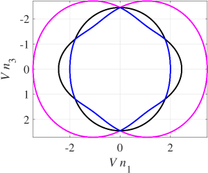
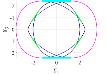
(c)	(d)

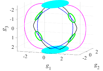
Figure 2: (a) Phase-velocity, (b) group-velocity, and (c) slowness surfaces of the P- (magenta), S₁- (black), and S₂-waves (blue) in the $[\bm{x}_{1},\,\bm{x}_{3}]$ plane of orthorhombic model 27. Figure (d) presents a 3D view of (b), displaying four bases $\bm{g}^{E}$ (the green lines) of the internal refraction cones related to conical singularities $\bm{n}^{s}=[\pm 0.832,\,0,\,\pm 0.555]$ in the symmetry plane $[\bm{x}_{1},\,\bm{x}_{3}]$ and two bases $\bm{g}^{Q}$ (the filled cyan ellipses) related to triple singularities at $\bm{n}^{t}=[0,\,0,\,\pm 1]$.

Figure 2, computed for an orthorhombic medium characterized by the stiffness matrix

$$\bm{c}=\left(\begin{array}[]{c c c c c c}12&3&0&0&0&0\\ {}\hfil&10&5&0&0&0\\ {}\hfil&{}\hfil&6&0&0&0\\ {}\hfil&\mathrm{SYM}&{}\hfil&6&0&0\\ {}\hfil&{}\hfil&{}\hfil&{}\hfil&6&0\\ {}\hfil&{}\hfil&{}\hfil&{}\hfil&{}\hfil&4\\ \end{array}\right)\!$$ (27)

obeying constraints 6bb, displays the bases of internal refraction cones corresponding to both triple (cyan) and shear-wave conical (green) singularities that can coexist in the same model.

A more intellectually pleasing and certainly more instructive example, illustrating the findings of section III, is shown in Figure 3 for a cubic (a special case of orthorhombic) model

$$\bm{c}=\left(\begin{array}[]{c c c c c c}1&0.9&0.9&0&0&0\\ {}\hfil&1&0.9&0&0&0\\ {}\hfil&{}\hfil&1&0&0&0\\ {}\hfil&\mathrm{SYM}&{}\hfil&1&0&0\\ {}\hfil&{}\hfil&{}\hfil&{}\hfil&1&0\\ {}\hfil&{}\hfil&{}\hfil&{}\hfil&{}\hfil&1\\ \end{array}\right)\!.$$ (28)

As can be easily verified, model 28 possesses triple singularities along all three coordinate axes $\bm{n}^{t_{1}}=[\pm 1,\,0,\,0]$, $\bm{n}^{t_{2}}=[0,\,\pm 1,\,0]$, and $\bm{n}^{t_{3}}=[0,\,0,\,\pm 1]$. According to equations 18, the phase velocities have to coincide for all singular directions $\bm{n}^{t_{i}}$ $(i=1,\,2,\,3)$,

$$V\!\left(\bm{n}^{t_{1}}\right)=V\!\left(\bm{n}^{t_{2}}\right)=V\!\left(\bm{n}^{t_{3}}\right),$$ (29)

and Figure 3a displays equality of the two velocities, $V\!\left(\bm{n}^{t_{1}}\right)=V\!\left(\bm{n}^{t_{3}}\right)=1$.

(a)	(b)
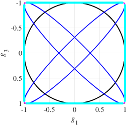
(c)	(d)

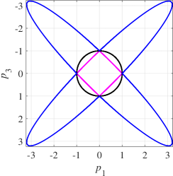
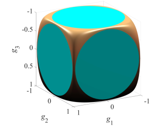
Figure 3: (a) – (c) Same as Figures 2a – 2c but for cubic stiffness matrix 28. Model 28 has no conical singularities in the $[\bm{x}_{1},\,\bm{x}_{3}]$ symmetry plane; the bases $\bm{g}^{E}$ of internal refraction cones at out of plane singularities $\bm{n}^{s}=[\pm 1,\,\pm 1,\,\pm 1]/\sqrt{3}$ are not shown. As in Figure 2, the filled cyan circles in (d) and their projections onto the plane $[\bm{x}_{1},\,\bm{x}_{3}]$ in (b) are the bases $\bm{g}^{Q}$ of internal refraction cones corresponding to triple singularities. 3D surface in (d) is the outer (P-wave) sheet of the group-velocity surface.

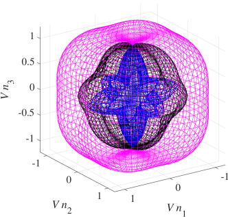
Figure 4: Phase-velocity sheets of the P- (magenta), S₁- (black), and S₂-waves (blue). The phase-velocity sheet of the S₁-wave is not a sphere even though its cross-section in the $[\bm{x}_{1},\,\bm{x}_{3}]$ plane is a circle (Figure 3a).

Because $c_{44}=c_{66}=1$ in stiffness matrix 28, the S₁- or SH-wave exhibits kinematically isotropic behavior in the vertical symmetry plane $[\bm{x}_{1},\,\bm{x}_{3}]$ (the black circles in Figure 3a – 3c), providing a convenient baseline for the visual confirmation of inequality 16. Figure 3a shows that the phase velocity of the P-wave (magenta) is greater than the phase velocity of the S₂-wave (blue) everywhere except for directions $\bm{n}^{t_{1}}$ and $\bm{n}^{t_{3}}$, along which the two phase velocities coincide,

$$V_{\mathrm{P}}(\bm{n}^{t_{1}})=V_{\mathrm{S2}}(\bm{n}^{t_{1}})=V_{\mathrm{P}}(\bm{n}^{t_{3}})=V_{\mathrm{S2}}(\bm{n}^{t_{3}})=1\,.$$ (30)

The same relationship holds for the entire P- and S₂-wave phase-velocity sheets in 3D (Figure 4), not just for their cross-sections by the $[\bm{x}_{1},\,\bm{x}_{3}]$ plane.

The equality of off-diagonal stiffness elements $c_{12}=c_{13}=c_{23}$ in matrix 28 degenerates quartic bases $\bm{g}^{Q}$ of all internal refraction cones to circles (see equations 25 and 26). These bases form planar patches at the group-velocity surfaces, shown in cyan in Figure 3d for the P-wave group-velocity sheet, exhibiting shape of a delightful dice.

Model 28 has three triple singularities. Next, we show that the maximum number of triple singularities — four — is also attainable.

The system of six equations 19 in orthorhombic media reads

$$\Gamma_{11}(\bm{p}^{t})=c_{11}\,(p^{t}_{1})^{2}+c_{66}\,(p^{t}_{2})^{2}+c_{55}\,(p^{t}_{3})^{2}=1\,,$$ (31a)

$$\Gamma_{12}(\bm{p}^{t})=(c_{12}+c_{66})\,p^{t}_{1}\,p^{t}_{2}=0\,,$$ (31b)

$$\Gamma_{13}(\bm{p}^{t})=(c_{13}+c_{55})\,p^{t}_{1}\,p^{t}_{3}=0\,,$$ (31c)

$$\Gamma_{22}(\bm{p}^{t})=c_{66}\,(p^{t}_{1})^{2}+c_{22}\,(p^{t}_{2})^{2}+c_{44}\,(p^{t}_{3})^{2}=1\,,$$ (31d)

$$\Gamma_{23}(\bm{p}^{t})=(c_{23}+c_{44})\,p^{t}_{2}\,p^{t}_{3}=0\,,$$ (31e)

$$\Gamma_{33}(\bm{p}^{t})=c_{55}\,(p^{t}_{1})^{2}+c_{44}\,(p^{t}_{2})^{2}+c_{33}\,(p^{t}_{3})^{2}=1\,.$$ (31f)

We satisfy equations 31fb, 31fc, and 31fe identically by imposing constraints on the stiffness coefficients

$$c_{12}=-c_{66}\,,$$ (32a)

$$c_{13}=-c_{55}\,,$$ (32b)

$$c_{23}=-c_{44}\,$$ (32c)

analogous to equations 6ba. Then the three remaining equations 31fa, 31fd, and 31ff, linear in the squared slowness components $(p^{t}_{i})^{2}$ $(i=1,\,2,\,3)$, can be solved analytically, yielding eight roots $\bm{p}^{t}$ with the components

$$p^{t}_{1}=\pm\frac{1}{d}\,\sqrt{c_{22}\,c_{33}-c_{22}\,c_{55}-c_{33}\,c_{66}+c_{44}\,(c_{55}+c_{66}-c_{44})}\,,$$ (33a)

$$p^{t}_{2}=\pm\frac{1}{d}\,\sqrt{c_{11}\,c_{33}-c_{11}\,c_{44}-c_{33}\,c_{66}+c_{55}\,(c_{44}+c_{66}-c_{55})}\,,$$ (33b)

$$p^{t}_{2}=\pm\frac{1}{d}\,\sqrt{c_{11}\,c_{22}-c_{11}\,c_{44}-c_{22}\,c_{55}+c_{66}\,(c_{44}+c_{55}-c_{66})}\,,$$ (33c)

where the denominators

$$d=\sqrt{c_{11}\,c_{22}\,c_{33}+2\,c_{44}\,c_{55}\,c_{66}-c_{11}\,c_{44}^{2}-c_{22}\,c_{55}^{2}-c_{33}\,c_{66}^{2}}\,.$$ (34)

As can be directly verified, the phase velocities $V_{t}$ coincide for all roots 33c,

$$V_{t}\equiv\frac{1}{|\bm{p}^{t}|}=d\! \Big{[}\,2\,(c_{44}\,c_{55}+c_{44}\,c_{66}+c_{55}\,c_{66}-c_{11}\,c_{44}-c_{22}\,c_{55}-c_{33}\,c_{66})$$ (35)

$$\,\,\,+\,c_{11}\,c_{22}+c_{11}\,c_{33}+c_{22}\,c_{33}-c_{44}^{2}-c_{55}^{2}-c_{66}^{2}\Big{]}^{-1/2}\,,$$

confirming our theoretical assertion 18.

Constructing an orthorhombic model for which the slowness components 33c are real-valued is not difficult. For example, a solid described by the stiffness matrix

$$\bm{c}=\left(\begin{array}[]{c c r c c c}7&-3&-2&0&0&0\\ {}\hfil&~{}~{}8&-1&0&0&0\\ {}\hfil&{}\hfil&9&0&0&0\\ {}\hfil&\mathrm{SYM}&{}\hfil&1&0&0\\ {}\hfil&{}\hfil&{}\hfil&{}\hfil&2&0\\ {}\hfil&{}\hfil&{}\hfil&{}\hfil&{}\hfil&3\\ \end{array}\right)\!,$$ (36)

satisfying conditions 32c, has four distinct triple singularities

$$\bm{n}^{t_{1}}=[+1,\,+1,\,+1]/\sqrt{3}\,,$$ (37a)

$$\bm{n}^{t_{2}}=[+1,\,+1,\,-1]/\sqrt{3}\,,$$ (37b)

$$\bm{n}^{t_{3}}=[+1,\,-1,\,+1]/\sqrt{3}\,,$$ (37c)

$$\bm{n}^{t_{4}}=[-1,\,+1,\,+1]/\sqrt{3}\,,$$ (37d)

directions of the two of them, $\bm{n}^{t_{1}}$ and $\bm{n}^{t_{2}}$, marked by the cyan arrows in Figure 5a.

The P-wave sheet of the group-velocity surface in Figure 5b displays another remarkable shape — two smooth square pyramids, connected together at their horizontal bases and symmetric with respect to the horizontal, as they should be to maintain the central symmetry of group-velocity surfaces. And like Figure 3d, the faces of the pyramids exhibit large planar patches, colored in cyan.

(a)	(b)

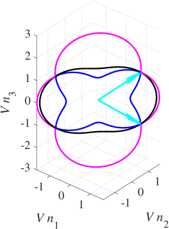
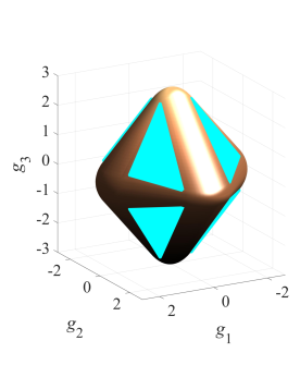
Figure 5: (a) Cross-sections of the phase-velocity surfaces of the P- (magenta), S₁- (black), and S₂-waves (blue) by the vertical plane oriented at $45^{\circ}$ with respect to the horizontal coordinate axes $\bm{x}_{1}$ and $\bm{x}_{2}$ and (b) the P-wave sheet of the group-velocity surface for orthorhombic model 36. The cyan arrows in (a) point to triple singularities $\bm{n}^{t_{1}}$ and $\bm{n}^{t_{2}}$ (equations 37da and 37db) in the cross-section plane, singularities $\bm{n}^{t_{3}}$ and $\bm{n}^{t_{4}}$ (equations 37dc and 37dd) are located in the vertical plane orthogonal to the cross-section. Similar to Figure 3d, the cyan patches in (b) are the planar bases $\bm{g}^{Q}$ of internal refraction cones formed at triple singularities.

VI Vertical transverse isotropy

The transition from triple singularities at the vertical in orthorhombic media to those in vertically transversely isotropic (VTI) media is straightforward. Because $c_{13}=c_{23}$ for vertical transverse isotropy, the internal refraction cone 24 is circular,

$$\bm{g}^{t}=\bm{g}(\bm{n}^{t},\,\varphi_{1},\,\varphi_{2})=\left[\begin{array}[]{c}\dfrac{c_{13}+c_{55}}{2\,V_{t}}\,\sin 2\,\varphi_{1}\,\cos\varphi_{2}\\ \dfrac{c_{13}+c_{55}}{2\,V_{t}}\,\sin 2\,\varphi_{1}\,\sin\varphi_{2}\\ V_{t}\end{array}\right]\!;$$ (38)

its horizontal base $\bm{g}^{Q}$ has a radius of

$$\max\left(g_{1}^{t}\right)=\max\left(g_{2}^{t}\right)=\dfrac{1}{2}\left(\dfrac{c_{13}}{V_{t}}+V_{t}\right)\!.$$ (39)

(a)	(b)

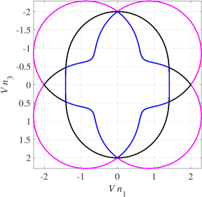
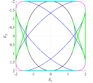
Figure 6: (a) Phase- and (b) group-velocity surfaces of the P- (magenta), S₁- (black), and S₂-waves (blue) in the $[\bm{x}_{1},\,\bm{x}_{3}]$ plane of VTI model 40. The bases $\bm{g}^{E}$ of degenerative internal refraction cones corresponding to the intersection singularities are displayed in green, the bases $\bm{g}^{Q}$ of internal refraction cones corresponding to the triple singularities at the vertical — in cyan.

Like triple and conical singularities in triclinic and orthorhombic solids, triple and intersection singularities can coexist in VTI media, as exemplified in Figure 6 computed for a model that has the stiffness matrix

$$\bm{c}=\left(\begin{array}[]{c c c c c c}4&0&2&0&0&0\\ {}\hfil&4&2&0&0&0\\ {}\hfil&{}\hfil&4&0&0&0\\ {}\hfil&\mathrm{SYM}&{}\hfil&4&0&0\\ {}\hfil&{}\hfil&{}\hfil&{}\hfil&4&0\\ {}\hfil&{}\hfil&{}\hfil&{}\hfil&{}\hfil&2\\ \end{array}\right)\!.$$ (40)

A notable feature of Figure 6b is an atypically small portion of the purely P-wave branch (magenta) of the total group-velocity surface, also observed in Figures 3b (magenta) and 3d (copper).

VII Discussion

Triple singularities, admittedly unusual objects, entailing the presence of finite-size planar patches on group-velocity surfaces, raise a valid question about practical importance of their mathematical possibility. Because the existence of triple singularities rests upon equality-type constraints (equations 6b) that can be destroyed by an arbitrary triclinic perturbation of the stiffness tensor, Alshits et al. (1985) suggested that “triple [singularities] do not occur.” The logic behind this statement is fascinating, linking it to the philosophical in some sense subject of the presence of anisotropic symmetries in rocks as opposed to those in crystals, where symmetry of a crystal inherits the exact symmetry of its atomic lattice. Because symmetry of a rock sample can be only approximate, and the concept of approximate symmetry is barely touched in the literature, it seems appropriate to briefly discuss it.

Elastic properties and symmetry of a volume of core or geologic formation can be computed given the precise knowledge of microstructure of the volume and the stiffness tensors $\bm{c}(\bm{x})$ at its physical points $\bm{x}$. The process of computing the overall or effective elastic properties, known as homogenization, has been covered in several booksNemat-Nasser and Hori (1999); Milton (2002); Kachanov et al. (2003) and applied to fractured solidsGrechka and Kachanov (2006a, b); Grechka et al. (2006); Grechka (2007a, b). Because rocks are composed of diverse anisotropic minerals that are not perfectly aligned and contain dry or fluid-filled pores and fractures, the overall symmetry of rocks usually comes out triclinic, as confirmed by suitable seismic dataDewangan and Grechka (2003); Grechka and Yaskevich (2014) and numerical experiments. Hence, the stiffness matrixes of solids with symmetries lower than triclinic should be deemed as mere approximations of a more complex reality. Yet, explicitly imposing equality-type constrains on the stiffness tensor to make it symmetric — orthorhombic, transversely isotropic, or even isotropic, as expressed by the zeros and coinciding elements in the corresponding stiffness matrixes — has proven extremely useful in numerous rock physics, seismic, and seismological applications. Therefore, the fact that an arbitrary triclinic perturbation breaks down elastic symmetries is irrelevant; and as long as an adopted symmetry, understood as an approximation, happens to be helpful in solving particular problems, its inexactness is not only acceptable but even desirable for simplifying the ensuing computations and conclusions.

Likewise, slight violation of constraints 6b, while formally destroying the triple singularity as a mathematical entity, would not alter seismic signatures in any significant way; and because P-to-S₁ singularities occur in certain types of woodsMusgrave (1970), the existence of materials exhibiting some semblance of triple singularities might be possible.

VIII Conclusions

The following features of triple singularities have been established.

• The group-velocity vectors at a triple singularity fill solid cones.

• These internal refraction cones are generally quartic, although they can degenerate to quadratic — elliptic or circular — in more symmetric solids than triclinic.

• The base of an internal refraction cone is planar, giving rise to planar patches shared by group-velocity surfaces of the P-, S₁-, and S₁-waves.

• The maximum number of triple singularities is equal to 4, smaller than that of conventional (double) singularities, known to be 16.

• If multiple triple singularities are present, the phase velocities along all of them are exactly equal.

IX Acknowledgments

I would like to thank Yuriy Ivanov for spotting typos in equations 10 and 11. The typos are now corrected.

References

- Fedorov (1968) F. I. Fedorov, Theory of elastic waves in crystals (Plenum Press, 1968).
- Alshits and Lothe (1979a) V. I. Alshits and J. Lothe, Soviet Physics, Crystallography 24, no. 4, 387 (1979a).
- Alshits and Lothe (1979b) V. I. Alshits and J. Lothe, Soviet Physics, Crystallography 24, no. 4, 393 (1979b).
- Crampin (1981) S. Crampin, Wave motion 3, 343 (1981).
- Crampin and Yedlin (1981) S. Crampin and M. Yedlin, Journal of Geophysics 49, 43 (1981).
- Musgrave (1981) M. J. P. Musgrave, Proceedings of the Royal Society of London, Series A, Mathematical and Physical Sciences 374, 401 (1981).
- Alshits et al. (1985) V. I. Alshits, A. V. Sarychev, and A. L. Shuvalov, Soviet Journal of the Experimental and Theoretical Physics 63, no. 3, 531 (1985).
- Helbig (1994) K. Helbig, Foundations of anisotropy for exploration seismics (Elsevier, 1994).
- Schoenberg and Helbig (1997) M. Schoenberg and K. Helbig, Geophysics 62, no. 6, 1954 (1997).
- Shuvalov (1998) A. L. Shuvalov, Proceedings of the Royal Society of London, Series A: Mathematical, Physical and Engineering Sciences 454, no. 1979, 2911 (1998).
- Boulanger and Hayes (1998) P. Boulanger and M. Hayes, Proceedings of the Royal Society of London, Series A 454, 2323 (1998).
- Vavryčuk (2001) V. Vavryčuk, Geophysical Journal International 145, no. 1, 265 (2001).
- Vavryčuk (2003) V. Vavryčuk, Geophysical Journal International 152, no. 2, 318 (2003).
- Vavryčuk (2005a) V. Vavryčuk, Journal of Acoustical Society of America 118, no. 2, 647 (2005a).
- Vavryčuk (2005b) V. Vavryčuk, Geophysical Journal International 163, no. 2, 629 (2005b).
- Alshits (2003) V. I. Alshits, Proceedings of the World Congress on Ultrasonics: WCU 2003 pp. 999–1006 (2003).
- Goldin (2013) S. V. Goldin, Geophysical Prospecting 61, 1084 (2013).
- Grechka (2015) V. Grechka, Geophysics 80, no. 1, C1 (2015).
- Grechka (2017) V. Grechka, Geophysics 82, no. 4, WA45 (2017).
- Ivanov (2019) Y. Ivanov, submitted to Geophysical Prospecting (2019).
- Christoffel (1877) E. B. Christoffel, Annali di Matematica 8, 193 (1877).
- Musgrave (1970) M. J. P. Musgrave, Crystal acoustics (Holden-Day, 1970).
- Tsvankin (2001) I. Tsvankin, Seismic signatures and analysis of reflection data in anisotropic media (Elsevier, 2001).
- Grechka (2009) V. Grechka, Applications of seismic anisotropy in the oil and gas industry (EAGE, 2009).
- Grechka and Obolentseva (1993) V. Grechka and I. R. Obolentseva, Geophysical Journal International 115, no. 3, 609 (1993).
- Vavryčuk and Yomogida (1996) V. Vavryčuk and K. Yomogida, Wave Motion 23, 83 (1996).
- Shuvalov and Every (1997) A. L. Shuvalov and A. G. Every, Journal of the Acoustical Society of America 101, 2381 (1997).
- Weisstein (2003) E. W. Weisstein, CRC concise encyclopedia of mathematics (Chapman & Hall/CRC, 2003).
- Nemat-Nasser and Hori (1999) S. Nemat-Nasser and M. Hori, Micromechanics: Overall properties of heterogeneous materials (Elsevier, 1999).
- Milton (2002) G. M. Milton, The theory of composites (Cambridge University Press, 2002).
- Kachanov et al. (2003) M. Kachanov, B. Shafiro, and I. Tsukrov, Handbook of elasticity solutions (Kluwer Academic Publishers, 2003).
- Grechka and Kachanov (2006a) V. Grechka and M. Kachanov, Geophysics 71, no. 6, W45 (2006a).
- Grechka and Kachanov (2006b) V. Grechka and M. Kachanov, Geophysics 71, no. 3, D85 (2006b).
- Grechka et al. (2006) V. Grechka, I. Vasconcelos, and M. Kachanov, Geophysics 71, no. 5, D153 (2006).
- Grechka (2007a) V. Grechka, International Journal of Fracture, Letters in Fracture and Micromechanics 144, 181 (2007a).
- Grechka (2007b) V. Grechka, Geophysics 72, no. 5, D81 (2007b).
- Dewangan and Grechka (2003) P. Dewangan and V. Grechka, Geophysics 68, 1022 (2003).
- Grechka and Yaskevich (2014) V. Grechka and S. Yaskevich, Geophysics 79, no. 1, KS1 (2014).