Role of zero point energy in promoting ice formation in a spherical drop of water

Abstract

We demonstrate that the Lifshitz interaction energy (excluding the self-energies of the inner and outer spherical regions) for three concentric spherical dielectric media can be evaluated easily using the immense computation power in recent processors relative to those of a few decades ago. As a prototype, we compute the Lifshitz interaction energy for a spherical shell of water immersed in water vapor of infinite extent while enclosing a spherical ball of ice inside the shell, such that two concentric spherical interfaces are formed: one between solid ice and liquid water and the other between liquid water and gaseous vapor. We evaluate the Lifshitz interaction energy for the above configuration at the triple point of water when the solid, liquid, and gaseous states of water coexist, and, thus, extend the analysis of Elbaum and Schick in Phys. Rev. Lett. 66 (1991) 1713 to spherical configurations. We find that, when the Lifshitz energy contributes dominantly to the total energy of this system, which is often the case when electrostatic interactions are absent, a drop of water surrounded by vapor of infinite extent is not stable at the triple point. This instability, that is a manifestation of the quantum fluctuations in the medium, will promote formation of ice in water, which will then grow in size indefinitely. This is a consequence of the finding here that the Lifshitz energy is minimized for large (micrometer size) radius of the ice ball and small (nanometer size) thickness of the water shell surrounding the ice. These results might be relevant to the formation of hail in thunderclouds. These results are tentative in that the self-energies are omitted; surface tension and nucleation energy are not considered.

I Introduction

The term Casimir effect is often used to refer to the entire phenomena associated with quantum fluctuations. Other closely related terminologies are quantum vacuum energy, zero point energy, Lifshitz energy, London dispersion forces, and van der Waals interactions. The ideas governing the van der Waals interactions van der Waals (1873) and London dispersion forces Eisenschitz and London (1930); London (1930); Hettema (2000) originated in attempts to understand the interactions of neutral, but polarizable, molecules of gases that deviated in their characteristics from the ideal gas law. Casimir and Polder Casimir and Polder (1948) later generalized these calculations to include retardation effects. The concept of zero point energy on the other hand originated in the 1910’s in works of Refs. Planck (1914); Einstein and Hopf (1910); Einstein and Stern (1913) where the focus was to understand the blackbody radiation Planck (1901) in the limit of zero temperature. A priori it was not expected that the theory of radiation would have anything to do with inter-atomic forces. However, the astonishing feat of Casimir Casimir (1948) was in showing that London dispersion forces, or the van der Waals interactions, were manifestations of the zero point energy.

Casimir evaluated the energy of a planar cavity with perfectly conducting walls, an overly idealized system, that is obtained from the configuration of Fig. 1 when the regions labeled as $\varepsilon_{1}$ and $\varepsilon_{2}$ are perfect electrical conductors that are separated by vacuum in the background region labeled $\varepsilon_{3}$. Lifshitz Lifshitz (1956) generalized Casimir’s result by evaluating the energy for a configuration of Fig. 1 consisting of two dielectric media of infinite extent separated by vacuum. The Lifshitz energy leads to the Casimir energy in the perfect conducting limit of the dielectric functions for the outer media. Dzyaloshinskii, Lifshitz, and Pitaevskii (DLP) Dzyaloshinskii et al. (1961) extended these considerations for the case when the background region in the planar configuration of Fig. 1 is another uniform dielectric medium. The main idea underlying these groundbreaking works is that quantum fluctuations of fields in the media can be manifested in physical phenomena involving dielectrics. Among these, we point out that the configurations considered by Casimir and Lifshitz always lead to an attractive pressure (tending to decrease the thickness of the intervening medium). In contrast, the configurations considered by DLP allows for the pressure to be attractive or repulsive.

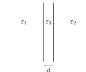
Figure 1: Three planar regions described by dielectric functions $\varepsilon_{1}$, $\varepsilon_{3}$, and $\varepsilon_{2}$, such that the thickness of the confined medium is $d$.

Elbaum and Schick Elbaum and Schick (1991a), using the result of DLP in conjunction with the existing data for the dielectric functions for ice and water, showed that an interface of solid ice and gaseous vapor is unstable at the triple point of water. They showed that quantum fluctuations in the electromagnetic fields in the media induces the formation of a 3.56 nm thick layer of liquid water at the interface, intervening between solid ice and gaseous vapor. The temperature of the triple point of water sets the scale for the energy of the system and the associated characteristic frequency obtained by dividing the energy by the Planck constant $\hbar$ corresponds to the frequency of the lowest Matsubara mode, equal to $2\pi k_{B}T/\hbar\approx 2.5\times 10^{14}$ rad/s. The source of the instability of the interface predicted by Elbaum and Schick was associated to the fact that solid ice is more polarizable than liquid water for frequencies larger than the 71st Matsubara mode, $\omega_{c2}\approx 71\times(2.5\times 10^{14}$ rad/s), while solid ice is less polarizable than liquid water for frequencies smaller than $\omega_{c2}$, and the static polarizability of solid ice is larger than that of liquid water. A remarkable feature of the Elbaum-Schick effect in water is that it necessarily requires taking retardation effects into consideration, that is, the effect disappears in a non-retarded analysis. This is striking because in planar configurations with vacuum as the background medium the retardation effects become relevant only when the thickness of the vacuum is hundreds of nanometer thick. However, if we introduce an intervening medium as done in the general configuration of DLP, it is possible to have retardation effects play a role at very small distances, the Elbaum-Schick effect being a classic example. This was already anticipated by DLP in the context of wetting of a wall. Recently in Ref. Thiyam et al. (2018a) this same idea was exploited to reverse the direction of torque as the separation distance between two anisotropic dielectric media is changed. We also verified that the Elbaum-Schick effect does not get washed away in the weak approximation, applicable for dilute dielectric media, which keeps the retardation effect and drops the higher order terms after expanding the logarithm in the expression for the Lifshitz energy.

It is important to emphasize that this effect cannot be thought of in terms of van der Waals energies, which refer to dilute, nonretarded limit. The effects we discuss in terms of the Lifshitz theory depend crucially on non-pairwise-additive forces and retardation. A Hamaker construction fails to capture the physics.

In this article we will evaluate the Lifshitz interaction energy, excluding the self-energies of the inner and outer dielectric regions. This calls for the definition of Lifshitz energy and some clarification on what we are not achieving in our calculations. To this end, we point out, though it has been surely known all along, that the energy for the configuration of Fig. 1 allows the decomposition Kenneth and Klich (2006); Shajesh and Schaden (2011):

$$E=E_{3}+\Delta E_{1}+\Delta E_{2}+E_{12}.$$ (1)

Here $E$ is the total energy; $E_{3}$ is the total energy when both interfaces are moved infinitely far away from each other to infinity, such that all space is filled with medium $\varepsilon_{3}$; $\Delta E_{1}=E_{1}-E_{3}$ and $\Delta E_{2}=E_{2}-E_{3}$ are self-energies required to create systems with single interfaces when the other interface is moved to $\pm\infty$ respectively; $E_{12}$ is the interaction energy between media $\varepsilon_{1}$ and $\varepsilon_{2}$. The interaction energy $E_{12}$ is the only contribution to the total energy that depends on the position and orientation of both media and determines the forces between them. This decomposition is generic, irrespective of $\varepsilon_{3}$ being vacuum or another medium. The importance of the decomposition of energy in Eq. (1) is the fact that the interaction energy $E_{12}$ is unambiguously finite by construction if media $\varepsilon_{1}$ and $\varepsilon_{2}$ are disjoint, even while the self-energies $\Delta E_{1}$, $\Delta E_{2}$, and $E_{3}$ remain divergent. Of considerable importance is the fact that self-energies may include the surface energies leading to surface tensions in the interfaces, however, due to the lack of predictive power in the face of divergences we will not discuss these terms in this article. The interaction energy $E_{12}$ is called the Lifshitz energy and this part of energy will be the subject matter of this article. The lack of a complete understanding to date of the divergent expressions in energy and omission of the associated contributions to energy all together here will remain a limitation of our analysis here.

Elbaum and Schick’s conclusion that quantum fluctuations induce the formation of a thin layer of liquid water at the interface of solid ice and gaseous vapor is valid for planar configurations. It is, then, of interest to inquire if these considerations change for curved geometries. In this article we extend the analysis of Elbaum and Schick to spherical concentric interfaces of solid ice, liquid water, and water vapor. We conclude that a spherical drop of water immersed inside gaseous vapor of infinite extent is unstable at the triple point of water. Quantum fluctuations promote formation of solid ice inside the drop of liquid water, which will then grow in size indefinitely. Once the solid ice has grown sufficiently large its surface can be approximated to that of a plane and in this limit the results of the planar configuration apply and the liquid water attains a thickness of 3.56 nm at equilibrium. The phenomena of quantum fluctuations promoting formation of ice in water, to our knowledge, has not been reported or mentioned in the literature before. This is expected to prompt a plethora of applications and studies associated to this phenomena, a few of which we mention in the last section and hope to explore in future publications.

A caveat must be stressed: We ignore the self-energies of each phase, as well as the associated surface tensions. We also realize that the energies involved here are very small compared to the nucleation energies. Surface tensions for the two interfaces involving water here are of order $10^{-1}$ J/m², while the energies resulting from the Lifshitz effects we consider are of order $10^{-7}$ J/m². So, we are considering quite small, but, we believe, significant effects.

Even though the expressions for Lifshitz energy (Helmholtz free energy) reported in this article are sufficiently general, we will consistently use solid ice for region 1 described by $\varepsilon_{1}$, liquid water for the background region $\varepsilon_{3}$, and gaseous water vapor for region 2 described by $\varepsilon_{2}$. The discussions in this article will be confined to the temperature and pressure associated with the triple point of water, $273.16\,$K and 611.657 Pa, when solid ice, liquid water, and water vapor, can coexist.

It should be emphasized that we are considering the quantum electrodynamic Casimir effect, due to the electrical properties of the materials, and not the thermodynamic critical Casimir effect Krech (1994), which is of quite a different character, and should not be relevant at the triple point, which is far from the critical point of water ($T_{c}=647$ K, $p_{c}=22$ MPa). At a critical point, as opposed to a triple point, the associated correlation length becomes infinite. Similarly, we have not accounted for the plausible fluctuations in surface imperfections. Thus, our discussion here is applicable for zero correlation lengths in the associated fluctuations.

II Elbaum-Schick effect

The Lifshitz interaction energy per unit area for the planar configuration of Fig. 1, consisting of three dielectric media with negligible magnetic permeabilities, $\mu_{i}=1$, such that the sandwiched medium has thickness $d$, is given by,

$${\cal E}(d) = \frac{\hbar c}{4\pi^{2}a_{0}}{\sum_{n=0}^{\infty}}{{}^{\prime}}\int_{0}^{\infty}kdk$$ (2)

$$\times\ln\left[1-r_{31}^{E}r_{32}^{E}e^{-2\kappa_{3}d}\right]\left[1-r_{31}^{H}r_{32}^{H}e^{-2\kappa_{3}d}\right],\hskip 8.53581pt$$

where the reflection coefficients for the transverse electric ($E$) and transverse magnetic ($H$) modes are given by

$$r_{ij}^{E}=-\left(\frac{\kappa_{i}-\kappa_{j}}{\kappa_{i}+\kappa_{j}}\right),\quad r_{ij}^{H}=-\left(\frac{\varepsilon_{j}\kappa_{i}-\varepsilon_{i}\kappa_{j}}{\varepsilon_{j}\kappa_{i}+\varepsilon_{i}\kappa_{j}}\right),$$ (3)

respectively, in terms of the effective refractive index

$$\kappa_{i}=\sqrt{k^{2}+\frac{n^{2}}{a_{0}^{2}}\varepsilon_{i}},\qquad i=1,3,2.$$ (4)

The prime on the summation symbol in Eq. (2) indicates that the $n=0$ term is to be multiplied by a factor of $1/2$. We have defined the constant

$$a_{0}=\frac{\hbar c}{2\pi k_{B}T}$$ (5)

with dimensions of length, which introduces a natural scale for distance in the discussion. The corresponding scale for energy is set by the coefficient $\hbar c/(4\pi^{2}a_{0})=k_{B}T/(2\pi)$ in Eq. (2). For typical dielectric materials at room temperature this distance $a_{0}$ is in the micrometer range corresponding to an energy in milli electron-volts. At the triple point of water the distance $a_{0}$ in Eq. (5) is evaluated to be

$$a_{0}=1.3342\,\mu\text{m}.$$ (6)

and the energy $\hbar c/(4\pi^{2}a_{0})=k_{B}T/(2\pi)$ in Eq. (2) equals 3.7463 meV.

II.1 Dielectric function

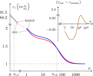
Figure 2: Dielectric functions of solid ice and liquid water, obtained using the fitting parameters used by Elbaum and Schick in Ref. Elbaum and Schick (1991a), plotted with respect to the Matsubara mode number $n$ ranging from 1 to 3700. The discrete frequency is $nc/a_{0}$, where $c/a_{0}=2.2470\times 10^{14}$ rad/s. The dielectric function at zero frequency ($n=0$) is huge and only sketched out for illustration, because it is hard to capture it on the same scale. The dielectric functions of solid ice and liquid water when extrapolated as a smooth line, even though they are actually discrete points, intersect at two points, first at $n_{c1}$ between $n=0$ and $n=1$, and then again at $n_{c2}$ between $n=71$ and $n=72$. The difference in the dielectric functions of solid ice and liquid water is plotted in the inset, where, again, the $n=0$ contribution is illustrated as a cartoon.

The permittivities $\varepsilon_{i}$ in Eqs. (3) and (4) are functions of the discrete imaginary frequency, the Matsubara frequency, $inc/a_{0}$,

$$\varepsilon_{j}=\varepsilon_{j}\left(in\frac{c}{a_{0}}\right),\qquad j=1,3,2.$$ (7)

The dielectric functions for $j=1,3,2,$ for solid ice, liquid water, and gaseous water vapor, respectively, are generated using the damped oscillator model for the dielectric response, following Elbaum and Schick Elbaum and Schick (1991a),

$$\varepsilon(\omega)=1+\sum_{j}\frac{f_{j}}{e_{j}^{2}-i\hbar\omega\,g_{j}-(\hbar\omega)^{2}},$$ (8)

where $e_{j}$, $f_{j}$, and $g_{j}$ are given by the values listed in Table 1 of Ref. Elbaum and Schick (1991a). The dielectric response at zero frequency for solid ice and liquid water are

$$\varepsilon_{\text{ice}}(0) = 91.5,$$ (9a)

$$\varepsilon_{\text{water}}(0) = 88.2,$$ (9b)

respectively. Data for dielectric functions were generated for $n$ spanning 0 to 3700, which were sufficient for convergence of the Lifshitz interaction energy in the regime of interest. The plots of these dielectric functions as a function of the Matsubara mode number $n$ are presented in Fig. 2. The dielectric function at zero frequency ($n=0$) for both ice and water is huge and could not be captured on the same scale, but, we sketched the intersection as a cartoon to illustrate the point. These plots, for solid ice and liquid water, intersect at two points, first at $n_{c1}$ between $n=0$ and $n=1$, and then again at $n_{c2}$ between $n=71$ and $n=72$. The difference in the dielectric functions of solid ice and liquid water, which plays a central role in our discussion, is plotted in the inset. Note, in particular, how the $n=0$ contribution for ice and water dwarfs the contribution from non-zero values.

II.2 Model dependence of dielectric functions

The results in this article are dependent on the intersections in Fig. 2. It is, then, of significance to investigate and quantify the sensitivity of the effect, discussed by Elbaum and Schick in Ref. Elbaum and Schick (1991a) and by us in this article, on the fitting parameters for the dielectric functions of solid ice and liquid water. Some of us with other collaborators have taken up this investigation separately, and thus it will have to be reported at a different venue. We content the reader by stating that the results seem to depend on the models. The results are sensitive to small changes in the dielectric functions for water and ice, originating from impurities, salts, or from improved models that incorporate a larger range of optical data Fiedler et al. (2019). This is not a limitation for this article, because the purpose of this article is to demonstrate that the Lifshitz interaction energy for concentric dielectric media can be evaluated easily, and the actual example we work out is only a prototype. However, our final results specific to the configuration of ice, water, and vapor, are indeed sensitive to the model parameters of the dielectric functions and thus are at best provisional.

II.3 Lifshitz energy for planar geometry

Using the model for the dielectric response in Eq. (8) for the fitting parameters used by Elbaum and Schick Elbaum and Schick (1991a), plotted in Fig. 2, the Lifshitz energy per unit area as a function of thickness $d$ of liquid water layer is plotted in Fig. 3. The Lifshitz energy diverges to positive infinity for zero thickness $d$ of liquid water, implying an instability of such an interface. That is, quantum fluctuations will induce the formation of a thin layer of liquid water at the interface of solid ice and gaseous vapor. The Lifshitz energy associated with two bodies, say two dielectric media separated by vacuum, diverges to negative infinity when the two media come in contact. Additionally, the Lifshitz energy goes to (positive) zero for large thickness. For intermediate distances the Lifshitz energy has a negative minimum for $d\sim 0.00267a_{0}\approx 3.56\,$nm. The existence of this minimum implies that at the triple point of water it is energetically favorable to form a layer of water at the interface of ice and vapor. In other words, an interface of solid ice and gaseous vapor is highly unstable because of the positive infinite energy associated with zero thickness of water in Fig. 3. At equilibrium the thickness of water formed at the interface is 3.56 nm.

The Lifshitz energy has a local maximum (positive) value of $0.0131\,{\cal E}_{0}$ when the thickness of water layer is $d\sim 0.275a_{0}\approx 0.37\,\mu\text{m}$, which is shown in the inset of Fig. 3. Thus, it is implied that the Lifshitz energy approaches zero from positive values of energy for large thickness of the water layer. This is consistent with the fact that at large distances the Lifshitz energy is completely characterized by the $n=0$ contribution. This observation, in principle, implies that complete melting of ice is possible if the water layer is thicker than $0.37\,\mu$m initially. However, the Lifshitz energy peaks here with a very tiny positive value of $0.0130\,{\cal E}_{0}$, which is very small relative to ${\cal E}_{0}=k_{B}T/(2\pi)/a_{0}^{2}$. Thus, complete melting is unlikely due to disturbances in energy from the surroundings.

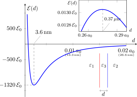
Figure 3: Lifshitz energy per unit area ${\cal E}(d)$ for liquid water of thickness $d$ sandwiched between solid ice and gaseous water vapor plotted as a function of $d$. The thickness $d$ is marked in units of $a_{0}=\hbar c/(2\pi k_{B}T)\approx 1.3342\,\mu$m, and the Lifshitz energy per unit area is marked in units of ${\cal E}_{0}=\hbar c/(4\pi^{2}a_{0}^{3})=k_{B}T/(2\pi)/a_{0}^{2}\approx 3.3720\times 10^{-10}$ J/m${}^{2}\approx 2.1046\times 10^{-11}$ eV/Ų. The Lifshitz energy has a minima at $d=3.56$ nm. The Lifshitz energy also has a maxima at $d=0.37\,\mu$m, which is shown in the inset-plot. The Lifshitz energy tends to zero from the positive side for large thickness, and goes to positive infinity for zero thickness.

Thus the Lifshitz energy has two extrema, a minimum at $d=3.56$ nm, and a maximum at $d=0.37\,\mu$m. These extremum points are roughly numerically estimated in terms of the two intersection points, $n_{c1}\sim 0.99$ and $n_{c2}=71$, in the plots of the dielectric functions of solid ice and liquid water in Fig. 2. We crudely estimated $n_{c1}\sim 0.99$ by assuming a linear interpolation between the data points at $n=0$ and $n=1$ in Fig. 2. The two intersection points in Fig. 2 correspond to frequencies

$$\omega_{ci}=n_{ci}\frac{c}{a_{0}},\qquad i=1,2,$$ (10)

which leads to

$$\omega_{c1} = 1.80\times 10^{14}\,\text{rad/s},$$ (11a)

$$\omega_{c2} = 1.60\times 10^{16}\,\text{rad/s}.$$ (11b)

In terms of these critical frequencies a rough numerical estimate of the extremum values for the thickness of water layer is obtained using Boström et al. (2017)

$$d_{i}\sim\frac{c}{\omega_{ci}}\frac{1}{2\sqrt{\varepsilon_{3}(i\omega_{ci})}},\qquad i=1,2.$$ (12)

This expression leads to $d_{1}\approx 0.41\,\mu$m and $d_{2}\approx 7.83$nm, which are in the right ballpark of $0.37\,\mu$m and $3.56$nm, respectively. We have been unable to find a more accurate analytical estimate, because we are dealing with a discrete function of the Matsubara mode numbers $n$, in addition to the fact that the zero mode behaves significantly differently from other modes Boström et al. (2017).

II.4 Incomplete surface melting

Melting of a solid into liquid at melting point $T_{m}$ is typically explained as a phase transition in thermodynamics. Another explanation proposed by Weyl in 1951 Weyl (1951) and theorized by Fletcher in 1968 Fletcher (1968) rests on a microscopic theory in which onset of melting happens at temperatures less than $T_{m}$. The proposal is that the energy of the ice or water surface is lowered when the dipole moments of the water molecules orient in assembly. This leads to the formation of an electric double layer at surfaces of water and ice. The electrostatic interactions of such surfaces, neglecting dispersion forces completely, led to a power law behavior of $d\sim t^{-1/3}$, where $t=1-(T/T_{m})$, $T<T_{m}$, for the thickness $d$ of liquid water formed on the surface of ice at temperatures slightly below the melting point. Thus, as the temperature approaches the melting point a thin layer of liquid water is formed at the surface which then grows to infinite thickness as the temperature approaches the melting point. These conclusions remain mostly the same even when non-retarded dispersion interactions are taken in account. This is called (complete) surface melting and seems to be a well studied microscopic explanation of melting. However, data from different experiments are not in concord with the specific power law behavior mentioned above Dash et al. (1995); Elbaum et al. (1995); Slater and Michaelides (2019).

The implication of Elbaum and Schick’s results in Ref. Elbaum and Schick (1991a) is that the surface melting for ice is incomplete. That is, the thickness of water layer remains finite as the temperature approaches the melting point. It was hard to confirm this accurately in the experiment by Elbaum et al. Elbaum et al. (1993). The challenge seems to be with determining the triple point of water precisely, and the formation of patches of water drops Elbaum et al. (1995) which probably could be associated with an unevenly flat surface of ice. We will explore the curvature dependence of Elbaum and Schick’s results in Sec. VI. Experimental confirmation of incomplete surface melting remains open Slater and Michaelides (2019).

III Lifshitz energy for concentric spherical geometry

The Casimir energy for a perfectly conducting spherical shell was first calculated by Boyer in 1968, which surprisingly had the opposite sign relative to the Casimir energy of two parallel plates Casimir (1953); Boyer (1968). The calculation was attempted for a dielectric ball in Ref. Milton (1980). However, irrespective of the particular regularization procedures used in the calculation, the $a_{2}$ heat kernel coefficient is nonzero, which seems to suggest that there is no way to make the Casimir energy of a dielectric ball finite, except for isorefractive cases ($\varepsilon\mu=1$) Brevik and Kolbenstvedt (1983). The understanding of this divergent phenomena associated with a single spherical interface is generally accepted to be unsatisfactory Milton (1980); Candelas (1982). These calculations evaluated the term $\Delta E_{1}$ in Eq. (1) for a spherical interface, with the background region chosen to be a homogeneous medium, which we pointed out give a divergent contribution. Here we calculate the interaction energy $E_{12}$ in Eq. (1) for the concentric spherical configuration in Fig. 4. The interaction energy $E_{12}$, by construction, is devoid of divergences and thus can be evaluated unambiguously. The concentric spherical configuration of Fig. 4, for the case when the inner and outer regions consist of identical material and the intervening region is vacuum, $\varepsilon_{1}=\varepsilon_{2}$ and $\varepsilon_{3}=1$, was studied first, and to our knowledge the only time in literature, by Brevik et al. Brevik et al. (2002a); Høye et al. (2001); Brevik et al. (2002b). However, the numerical estimates reported there were not satisfactory probably because the necessary convergence was not achievable with the computational power in the computers of those days. Our expression for the interaction energy here is a straightforward generalization of that in Refs. Brevik et al. (2002a); Høye et al. (2001); Brevik et al. (2002b), obtained by keeping all three regions in Fig. 4 distinct. In addition we report comprehensive numerical estimates for the interaction energy for the particular example of ice, water, and vapor, which can be easily reproduced for other cases using the methods prescribed here. In Ref. Parashar et al. (2017), the interaction energy for concentric spherical configurations constructed from $\delta$-function spheres were reported, which is different from the study here. We emphasize that we are not including the self-energies of the interior and exterior regions, which leads to an unknown systematic error.

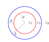
Figure 4: Three concentric spherical regions described by dielectric functions $\varepsilon_{1}$, $\varepsilon_{3}$, and $\varepsilon_{2}$, separated by the interfaces at radii $a$ and $b=a+d$.

For the spherical geometry of Fig. 4 with interfaces at radii $a$ and $b$ the Lifshitz energy $E(a,b)$ is given by Parashar et al. (2017); Shajesh et al. (2017)

$$E(a,b) = k_{B}T{\sum_{n=0}^{\infty}}{{}^{\prime}}\sum_{l=0}^{\infty}(2l+1)$$ (13)

$$\times\ln\left[1-r_{31}^{E}(a)r_{32}^{E}(b)\right]\left[1-r_{31}^{H}(a)r_{32}^{H}(b)\right],\hskip 14.22636pt$$

where the various scattering coefficients are given by

$$r_{31}^{E}(a) = \frac{\zeta_{3}\,\text{i}_{l}(\zeta_{1}a)\bar{\text{i}}_{l}(\zeta_{3}a)-\zeta_{1}\,\bar{\text{i}}_{l}(\zeta_{1}a)\text{i}_{l}(\zeta_{3}a)}{\zeta_{3}\,\text{i}_{l}(\zeta_{1}a)\bar{\text{k}}_{l}(\zeta_{3}a)-\zeta_{1}\,\bar{\text{i}}_{l}(\zeta_{1}a)\text{k}_{l}(\zeta_{3}a)},$$ (14a)

$$r_{31}^{H}(a) = \frac{\zeta_{1}\,\text{i}_{l}(\zeta_{1}a)\bar{\text{i}}_{l}(\zeta_{3}a)-\zeta_{3}\,\bar{\text{i}}_{l}(\zeta_{1}a)\text{i}_{l}(\zeta_{3}a)}{\zeta_{1}\,\text{i}_{l}(\zeta_{1}a)\bar{\text{k}}_{l}(\zeta_{3}a)-\zeta_{3}\,\bar{\text{i}}_{l}(\zeta_{1}a)\text{k}_{l}(\zeta_{3}a)},$$ (14b)

$$r_{32}^{E}(b) = \frac{\zeta_{2}\,\text{k}_{l}(\zeta_{3}b)\bar{\text{k}}_{l}(\zeta_{2}b)-\zeta_{3}\,\bar{\text{k}}_{l}(\zeta_{3}b)\text{k}_{l}(\zeta_{2}b)}{\zeta_{2}\,\text{i}_{l}(\zeta_{3}b)\bar{\text{k}}_{l}(\zeta_{2}b)-\zeta_{3}\,\bar{\text{i}}_{l}(\zeta_{3}b)\text{k}_{l}(\zeta_{2}b)},$$ (14c)

$$r_{32}^{H}(b) = \frac{\zeta_{3}\,\text{k}_{l}(\zeta_{3}b)\bar{\text{k}}_{l}(\zeta_{2}b)-\zeta_{2}\,\bar{\text{k}}_{l}(\zeta_{3}b)\text{k}_{l}(\zeta_{2}b)}{\zeta_{3}\,\text{i}_{l}(\zeta_{3}b)\bar{\text{k}}_{l}(\zeta_{2}b)-\zeta_{2}\,\bar{\text{i}}_{l}(\zeta_{3}b)\text{k}_{l}(\zeta_{2}b)},\hskip 14.22636pt$$ (14d)

in terms of the shorthand notation

$$\zeta_{i}=\frac{n}{a_{0}}\sqrt{\varepsilon_{i}\left(i\,n\frac{c}{a_{0}}\right)},\quad i=1,3,2.$$ (15)

The temperature dependent constant $a_{0}$ that appears in Eq. (15) was introduced in Eq. (5). The reflection coefficients are expressed in terms of the modified spherical Bessel functions $\text{i}_{l}(t)$ and $\text{k}_{l}(t)$ that are related to the modified Bessel functions by the relations

$$\text{i}_{l}(t) =\sqrt{\frac{\pi}{2t}}I_{l+\frac{1}{2}}(t),$$ (16a)

$$\text{k}_{l}(t) =\sqrt{\frac{\pi}{2t}}K_{l+\frac{1}{2}}(t).$$ (16b)

In particular $\text{i}_{l}(t)=\text{i}^{(1)}_{l}(t)$, the modified spherical Bessel function of the first kind, together with $\text{k}_{l}(t)$ are a suitable pair of solutions in the right half of the complex plane DLMF ; NIS (2010). The respective functions with a bar are the generalized derivatives of the modified spherical Bessel functions given by

$$\bar{\text{i}}_{l}(t) =\bigg{(}\frac{1}{t}+\frac{\partial}{\partial t}\bigg{)}\text{i}_{l}(t),$$ (17a)

$$\bar{\text{k}}_{l}(t) =\bigg{(}\frac{1}{t}+\frac{\partial}{\partial t}\bigg{)}\text{k}_{l}(t).$$ (17b)

Using the Wronskian for the modified spherical Bessel functions,

$$\text{k}_{l}\text{i}_{l}^{\prime}-\text{i}_{l}\text{k}_{l}^{\prime}=\frac{\pi}{2t^{2}},$$ (18)

where primes denote differentiation, we have the relation

$$\text{k}_{l}\bar{\text{i}}_{l}-\text{i}_{l}\bar{\text{k}}_{l}=\frac{\pi}{2t^{2}}.$$ (19)

The reflection coefficients are frequently expressed in terms of the modified Riccati-Bessel functions,

$$s_{l}(t) =t\,\text{i}_{l}(t),$$ (20a)

$$e_{l}(t) =\frac{2t}{\pi}\,\text{k}_{l}(t),$$ (20b)

whose derivatives can be expressed in the form

$$s_{l}^{\prime}(t) =t\,\bar{\text{i}}_{l}(t),$$ (21a)

$$e_{l}^{\prime}(t) =\frac{2t}{\pi}\,\bar{\text{k}}_{l}(t).$$ (21b)

For completeness we have provided the derivation of the Lifshitz energy for concentric spherical configurations, given in Eq. (13), in the Appendix.

IV Asymptotic expansions

Consider the scenario in which we know the dielectric functions in Eq. (7), for the three media in Fig. 4, as a function of Matsubara mode number $n$ to a reasonable accuracy. The computation of the interaction energy in Eq. (13) then, in principle, involves the evaluation of the sums over the Matsubara mode number $n$ and the angular momentum mode number $l$. Both these sums contribute negligibly for large values of $n$ and $l$. However, the reflection coefficients in Eqs. (14) involve ratios of differences, and these differences get exceedingly small for larger values of $l$. Thus, one has to keep an excessive number of significant digits in the evaluation of the Bessel functions, which is computationally expensive. This difficulty is avoided by expressing the modified Bessel functions using (uniform) asymptotic expansions for large order DLMF ; NIS (2010).

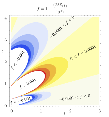
Figure 5: Contour plot of fractional error $f$ in estimating modified spherical Bessel function $\text{i}_{l}(t)$ using uniform asymptotic expansions. The errors are less than one percent for $l<2$ and $t<3$, however, these errors add up when we sum many terms.

The uniform asymptotic expansions for the modified spherical Bessel functions are written using the definitions

$$\nu=l+\frac{1}{2},\quad z=\frac{t}{\nu},\quad p(z)=\frac{1}{\sqrt{1+z^{2}}},$$ (22)

and

$$\eta(z)=\sqrt{1+z^{2}}+\ln\left(\frac{z}{1+\sqrt{1+z^{2}}}\right),$$ (23)

such that

$$\text{i}_{l}(t) \sim\sqrt{\frac{p}{z}}\,\frac{e^{\nu\eta(z)}}{2\nu}\,A_{\nu}(p),$$ (24a)

$$\text{k}_{l}(t) \sim\pi\sqrt{\frac{p}{z}}\,\frac{e^{-\nu\eta(z)}}{2\nu}\,B_{\nu}(p),$$ (24b)

$$\bar{\text{i}}_{l}(t) \sim\sqrt{\frac{1}{pz^{3}}}\,\frac{e^{\nu\eta(z)}}{2\nu}\,C_{\nu}(p),$$ (24c)

$$\bar{\text{k}}_{l}(t) \sim-\pi\sqrt{\frac{1}{pz^{3}}}\,\frac{e^{-\nu\eta(z)}}{2\nu}\,D_{\nu}(p),$$ (24d)

where

$$A_{\nu}(p) \sim\sum_{k=0}^{\infty}\frac{u_{k}(p)}{\nu^{k}},$$ (25a)

$$B_{\nu}(p) \sim\sum_{k=0}^{\infty}(-1)^{k}\frac{u_{k}(p)}{\nu^{k}},$$ (25b)

$$C_{\nu}(p) \sim\sum_{k=0}^{\infty}\frac{v_{k}(p)}{\nu^{k}}+\frac{p}{2\nu}\sum_{k=0}^{\infty}\frac{u_{k}(p)}{\nu^{k}},$$ (25c)

$$D_{\nu}(p) \sim\sum_{k=0}^{\infty}(-1)^{k}\frac{v_{k}(p)}{\nu^{k}}-\frac{p}{2\nu}\sum_{k=0}^{\infty}(-1)^{k}\frac{u_{k}(p)}{\nu^{k}},$$ (25d)

are expressed in terms of polynomials generated by

$$u_{k+1}(p) = \frac{p^{2}(1-p^{2})}{2}u_{k}^{\prime}(p)+\int_{0}^{p}dq\frac{(1-5q^{2})}{8}u_{k}(q),$$ (26a)

$$v_{k+1}(p) = u_{k+1}(p)+p(p^{2}-1)\left[\frac{u_{k}(p)}{2}+pu_{k}^{\prime}(p)\right],\hskip 28.45274pt$$ (26b)

with $u_{0}(p)=1$ and $v_{0}(p)=1$. The use of $\sim$ in place of equal sign in the equations suggest that these involve asymptotic series and the sums do not converge. The fractional error associated with using the uniform asymptotic expansions for the modified spherical Bessel functions in Eqs. (24) is plotted in Fig. 5 for order $l$ and argument $t$. The fractional errors are small and the largest error is only a percent for $l<2$ and $t<3$. Nevertheless, these errors could add up to significant levels in the computation of energy. This accumulation of error can be avoided in some cases by keeping more terms in inverse powers of $\nu$ in the sum on $k$, which is again computationally expensive.

Using the uniform asymptotic expansions for the modified spherical Bessel functions in Eqs. (24) we derive the corresponding expansions for the reflection coefficients in Eqs. (14) to be

$$r_{31}^{E}(a) \sim -\dfrac{1}{\pi}e^{2\nu\eta(\zeta_{3}a/\nu)}\dfrac{p_{1}A_{\nu}(p_{1})C_{\nu}(p_{3})-p_{3}C_{\nu}(p_{1})A_{\nu}(p_{3})}{p_{1}A_{\nu}(p_{1})D_{\nu}(p_{3})+p_{3}C_{\nu}(p_{1})B_{\nu}(p_{3})}\Bigg{|}_{p_{i}=p(\zeta_{i}a/\nu)},$$ (27a)

$$r_{31}^{H}(a) \sim -\dfrac{1}{\pi}e^{2\nu\eta(\zeta_{3}a/\nu)}\dfrac{\zeta_{1}^{2}p_{1}A_{\nu}(p_{1})C_{\nu}(p_{3})-\zeta_{3}^{2}p_{3}C_{\nu}(p_{1})A_{\nu}(p_{3})}{\zeta_{1}^{2}p_{1}A_{\nu}(p_{1})D_{\nu}(p_{3})+\zeta_{3}^{2}p_{3}C_{\nu}(p_{1})B_{\nu}(p_{3})}\Bigg{|}_{p_{i}=p(\zeta_{i}a/\nu)},$$ (27b)

$$r_{32}^{E}(b) \sim \pi e^{-2\nu\eta(\zeta_{3}b/\nu)}\dfrac{p_{3}B_{\nu}(p_{3})D_{\nu}(p_{2})-p_{2}D_{\nu}(p_{3})B_{\nu}(p_{2})}{p_{3}A_{\nu}(p_{3})D_{\nu}(p_{2})+p_{2}C_{\nu}(p_{3})B_{\nu}(p_{2})}\Bigg{|}_{p_{i}=p(\zeta_{i}b/\nu)},$$ (27c)

$$r_{32}^{H}(b) \sim \pi e^{-2\nu\eta(\zeta_{3}b/\nu)}\dfrac{\zeta_{3}^{2}p_{3}B_{\nu}(p_{3})D_{\nu}(p_{2})-\zeta_{2}^{2}p_{2}D_{\nu}(p_{3})B_{\nu}(p_{2})}{\zeta_{3}^{2}p_{3}A_{\nu}(p_{3})D_{\nu}(p_{2})+\zeta_{2}^{2}p_{2}C_{\nu}(p_{3})B_{\nu}(p_{2})}\Bigg{|}_{p_{i}=p(\zeta_{i}b/\nu)}.$$ (27d)

The zero Matsubara mode, $n=0$, requires special consideration, and is evaluated to be

$$r_{31}^{E}(a)r_{32}^{E}(b)\Big{|}_{n=0} = 0,$$ (28a)

$$r_{31}^{H}(a)r_{32}^{H}(b)\Big{|}_{n=0} = -l(l+1)\left(\frac{a}{b}\right)^{2l+1}\frac{[\varepsilon_{1}(0)-\varepsilon_{3}(0)]}{[l\varepsilon_{1}(0)+(l+1)\varepsilon_{3}(0)]}\frac{[\varepsilon_{3}(0)-\varepsilon_{2}(0)]}{[l\varepsilon_{2}(0)+(l+1)\varepsilon_{2}(0)]}.$$ (28b)

Using these uniform asymptotic expansions for large order for the reflection coefficients for non-zero Matsubara modes in Eqs. (27) and the explicit evaluation of the zero Matsubara mode in Eq. (28), in the expression for Lifshitz energy in Eq. (13), we successfully circumvent the difficulty posed with numerically evaluating quantities that involve very small numbers.

V Numerical Procedure

Table 1: Numerical data for the Lifshitz interaction energy $E(a,b)$, in Eq. (13), in units of $E_{0}=k_{B}T/(2\pi)=\hbar c/(4\pi^{2}a_{0})$, for three concentric dielectric regions, demarcated by radii $a$ and $b=a+d$, are catalogued with the respective $l_{\text{max}}$ and $n_{\text{max}}$ to obtain convergence and confidence in the necessary significant digits. Here $a_{0}=\hbar c/(2\pi k_{B}T)$, which at $T=273.16$ K yields $a_{0}\approx 1.3342\,\mu$m and $E_{0}=k_{B}T/(2\pi)\approx 6.0023\times 10^{-22}\,\text{J}\approx 3.7463\,\text{meV}$. The numbers displayed in the tiny font in each box denote ($l_{\text{max}}$, $n_{\text{max}}$, time, significant digits), for ice-water-vapor configuration. The maximum values for $l$ and $n$ are the values needed for the energy values to converge to the required significant digits. The time displayed is that for a typical personal computer.

The series in $l$ and $m$ are slowly converging even after employing uniform asymptotic expansions. We do not use any existing algorithms to speed up this slow convergence. We simply sum the terms. Nevertheless, we report the procedure in detail here for the sake of reproducibility. The numerical work presented here is not state of the art, and can be improved.

Our primary purpose in this article is to demonstrate that the Lifshitz energy for concentric spherical configurations can be computed easily. To this end, as an illustrative example, we consider a configuration consisting of solid ice inside liquid water inside water vapor in the configuration of Fig. 4.

To compute the numerical value for the Lifshitz energy in Eq. (13) we use the uniform asymptotic expansions for the reflection coefficients given in Eqs. (27), instead of the exact expressions for the reflection coefficients in Eqs. (14). This involves a sum on the Matsubara mode $n$, a sum on the angular momentum mode $l$, and multiple sums on $k$ to generate the energy. All these sums run from 0 to infinity, but only an optimal number of terms are to be included to avoid the unavoidable divergence associated with these asymptotic series. Further, numerical computation can not sum infinite terms, and dropping terms after an upper limit in the sums introduces only an acceptable error. In this article we shall obtain convergence and confidence in the numerical estimate up to three significant digits.

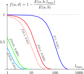
Figure 6: Convergence of energy $E(a,b)$ to a fixed value, during its computation. This is illustrated by plotting the fraction $f(a,d)$ as a function of the number of terms $l_{\text{max}}$ in the sum on $l$. Recall $b=a+d$. The numbers in the labels for the plot are in units of $a_{0}$.

We shall globally at the outset set an upper limit in sums on $k$ of inverse powers of $\nu=l+1/2$ for the asymptotic expansions to be $k_{\text{max}}=3$. It will be convenient to similarly set a global upper limit for the sum on the Matsubara mode number, $n_{\text{max}}$, and for the sum on the angular momentum mode, $l_{\text{max}}$. However, we learned that the required upper limit varies widely for the different combinations of the radii $a$ and $b$. For example, for the case when the inner radius of the sphere is large and the difference in the outer and inner radii is small, the sums on $n$ and $l$ in the interaction energy of Eq. (13) need to be evaluated at least until $n_{\text{max}}=2000$ and $l_{\text{max}}=6000$ to obtain convergence and confidence in the data up to three significant digits. Computationally this amounts to adding $n_{\text{max}}\times l_{\text{max}}=12\times 10^{6}$ terms in Eq. (13). A typical personal computer takes about one millisecond to evaluate one term in Eq. (13). To be specific, we used a computer with processor Intel Core i7-4700MQ CPU @ 2.40 GHz $\times$ 8, memory of 7.6 GB, which amounts to about 100 GFLOPS, and used Wolfram Mathematica Inc. for evaluation. Mathematica was preferred over other programs because of the convenience to invoke libraries of special functions. Thus, it takes a total of three hours to evaluate the energy for one particular configuration. The estimate for this time reduces by half if the demand in accuracy is brought down to two significant digits. To study the dependence of the energy in the two radii one needs to at least compute the energy on a $10\times 10$ array in the two radii. This amounts to three hundred hours of computation. Though it is not impractical to proceed ahead, such long computation hours makes the analysis tedious and inconvenient. Nevertheless, the difficulty in calculating the energy for a particular configuration is not as arduous as portrayed above. One makes the observation that the computational burden is considerably lower because the values of $n_{\text{max}}$ and $l_{\text{max}}$ needed for the necessary accuracy are significantly smaller for spherical configurations of smaller radii.

Our strategy was to catalogue the $n_{\text{max}}$ and $l_{\text{max}}$ for all possible combinations of the radii. This involves multiple runs to verify the convergence. However, once catalogued it helps the analysis tremendously, because only a small sector in the array is expensive on computational power. The catalogue for the ice-water-vapor configuration has been prepared in Table 1. We observe that the time taken to evaluate the energy for a particular configuration is most often negligible. It is only when the inner radii is large and difference in the radii is small that the time is painstakingly long. The energies in Table 1 are reported in units of $E_{0}=k_{B}T/(2\pi)=\hbar c/(4\pi^{2}a_{0})$ which is about 3.7463 meV at the triple point of water, $T=273.16$ K. We illustrate the convergence of the energy for a particular values of $a$ and $d$ as a function of the choice in $l_{\text{max}}$ in Fig. 6. The convergence in energy is computationally expensive in the bottom right corner of the chart in Table 1.

We made checks on the energies evaluated using uniform asymptotic expansions for the modified spherical Bessel functions by comparing it with values for energy obtained using the Bessel functions defined in Mathematica. Remarkably, to within three significant digits, the two results are identical for the parameter space used in this study. We verified this extensively for most of the parameter space, except for the few cases with large radii of ice and small thickness of water for which case the uniform asymptotic expansions fares very well.

It should be emphasized that the $l_{\text{max}}$ and $n_{\text{max}}$ presented in Table 1 is specific to the ice-water-vapor geometry. We expect the specific numbers to be different for another set of dielectric materials. However, we expect the pattern to be similar. That is, for all materials larger inner radii and small difference in radii will require the most computational effort.

VI Elbaum-Schick effect in spherical geometry

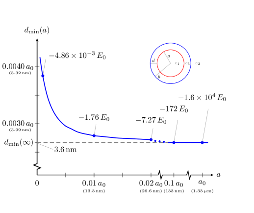
Figure 7: For a spherical shell of water, immersed in vapor and enclosing a ball of ice of radius $a$, at the triple point of water, we plot the thickness $d_{\text{min}}(a)$ of the shell of water that minimizes the Lifshitz energy for fixed $a$. The equilibrium thickness of the water layer, $d_{\text{min}}(a)$, is the least for large ice balls and increases for small radii of ice balls. The equilibrium thickness of water for the planar configuration $d_{\text{min}}(\infty)$ is achieved to within $1\,\%$ for ice ball of radius 20 nm. The corresponding Lifshitz energy at equilibrium is marked on the plot. The Lifshitz energy is minimum for large radii of ice. For reference, $a_{0}\approx 1.33\,\mu\text{m}$ at the triple point of water and $E_{0}=k_{B}T/(2\pi)=\hbar c/(4\pi^{2}a_{0})\approx 6.0023\times 10^{-22}\,\text{J}\approx 3.7463\,\text{meV}$.

In Sec. II we summarized how Elbaum and Schick in Ref. Elbaum and Schick (1991a) showed that at the triple point of water, at equilibrium, it is energetically favorable to form a $3.6$ nm thick layer of liquid water at a planar interface of solid ice and water vapor. We shall use $d_{\text{min}}(\infty)$ to denote this thickness. This is a delicate effect due to the fine differences in the frequency dependent polarizabilities of ice and water and their interplay in the presence of quantum fluctuations. It is also a relativistic effect in the sense that the effect is washed out if the analysis does not accommodate retardation. We inquire if the formation of a thin layer of water at the interface of ice and vapor will be disturbed if the ice-vapor interface were curved. In Sec. II.4 we pointed out that difficulties in the experimental verification of incomplete surface melting in the experiment by Elbaum et al. Elbaum et al. (1993) could be due to an unevenly flat interface. Thus, the curvature dependence of the incomplete surface melting is desired.

We investigate if it is energetically favorable to form a layer of water on the surface of solid ice in the shape of a sphere of radius $a$ when it is immersed in water vapor of infinite extent at the triple point of water. We find that a ball of solid ice at the triple point of water, at equilibrium, permits a thicker layer of water to be formed on its surface, relative to perfectly flat surface analyzed by Elbaum and Schick. In Fig. 7 we plot the thickness of liquid water at equilibrium $d_{\text{min}}(a)$ as a function of the radius of the ice ball $a$. We observe that a ball of ice of 20 nm radius is large enough that in this context we can assume its surface to be sufficiently flat for it to permit a water layer of thickness $d_{\text{min}}(\infty)$ to within 1% accuracy, with the strength of instability decided by the binding energy of about $-5E_{0}$. Here $E_{0}=k_{B}T/(2\pi)$ is a measure of the quantum of energy available in the heat bath surrounding the system.

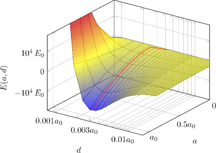
Figure 8: Lifshitz interaction energy $E(a,b)$, in Eq. (13), in units of $E_{0}=k_{B}T/(2\pi)=\hbar c/(4\pi^{2}a_{0})$, for three concentric dielectric regions, demarcated by radii $a$ and $b=a+d$, such that inner medium represents solid ice, the intermediate medium is liquid water, and the outer medium is water vapor, plotted as a function of $a$ and $d=b-a$. Here $a_{0}=\hbar c/(2\pi k_{B}T)$ is about $1.3342\,\mu\text{m}$ at the triple point of water. The red curve on the energy surface represents the thickness of water layer at equilibrium, $d_{\text{min}}(a)$, plotted in Fig. 7 separately.

In Fig. 7 the smallest radius of the ball of ice we consider is 1.33 nm ($0.001\,a_{0}$). In the range of radii we have studied the thickness of water layer formed at equilibrium monotonously increases for smaller radii of ice. Extrapolating this behavior to zero radii of ice we conclude that a water layer of infinite thickness is favored for small radii. The divergence associated with $a\to 0$ is very weak and consistent with our heuristic estimate $d_{\text{min}}=-\ln(\bar{\omega}_{c2}a)/{\bar{\omega}_{c2}}$ for $a\ll d$, where $\bar{\omega}_{c2}=2\omega_{c2}\sqrt{\varepsilon_{3}(i\omega_{c2})}$, similar to the estimate for the planar case in Eq. (12). In Fig. 7 we also mark the energies associated with each configuration. We observe that for radii of ice less than 10 nm the energy associated with the strength of instability is less than the quantum of energy available in the surrounding heat bath, which means that for these cases the disturbances in the surroundings will disturb the system and the conclusions of Fig. 7 are not relevant. To gain a better insight of the preference in energy we plot the Lifshitz interaction energy $E(a,b)$ as a function of both the radii of ice $a$ and the thickness of the water layer $d$ as a three dimensional plot in Fig. 8. We also overlap the curve representing $d_{\text{min}}(a)$ in Fig. 7 as a red curve on the energy surface in Fig. 8 for visual assistance. For most part this curve remains constant in $d$ in the scale of Fig. 8 and starts diverging for small radii of ice. Slices in the three dimensional plot of Fig. 8 representing fixed $a$ are energy plots whose minima are $d_{\text{min}}(a)$.

VI.1 Promotion of ice formation in water

In Fig. 8 it is clear that the configuration of minimum energy is for large radius of ice with a water layer having a thickness $d_{\text{min}}(\infty)$. We also conclude that a spherical drop of water inside an infinite extent of vapor with no ice inside the water has zero interaction energy, which can be concluded by extrapolating the energies on the curve in Fig. 7. This verifies that the Lifshitz interaction energy of Eq. (13) is zero for $a=0$, or for $d\to\infty$. Thus, a drop of water surrounded by vapor at the triple point of water is not stable. If ice is nucleated, the effects we consider will help promote the growth in size of the ice region indefinitely with the water layer thickness approaching $d_{\text{min}}(\infty)$.

An extrapolation leads to the hypothesis that zero point energy could induce nucleation of ice in water. This is a remarkable proposition, because the common wisdom is that ice nucleation requires an impurity like dust or soot or bacteria. The suggestion is that quantum fluctuations could contribute to inducing nucleation of ice even in the absence of impurities. However, the inward directed tension force on a small sphere is strong, and considerable energy is required in order to make nucleation possible. For a recent article on nucleation, one may consult Ref. Espinosa et al. (2019) and further references therein.

VI.2 Superheating and supercooling

Superheating of solids is the suspension of melting above the melting point. Stranski in 1942 Stranski (1942) argued that since superheating of solids is rarely observed the surface of solids must be wetted by its liquid phase. This argument is consistent with the idea of surface melting.

Supercooling of liquids is the absence of freezing below the melting point. In striking contrast supercooling of liquids is very common. It is well known that supercooled water can exist as small droplets in clouds. This seems to be consistent with the conclusion that zero point energy alone is insufficient to induce nucleation of ice in a water drop. However, the promotion of ice growth by the Lifshitz effect is more pronounced for a big drop of water because of the relatively large binding energy in Fig. 8, while for small drops of water of 10 nm and below the binding energy is too low and less than the quantum of energy available in the surrounding heat bath. Thus, it seems it should be easier to supercool small droplets of water and harder to supercool big drops of water, which is consistent with the observations.

VI.3 Proximity force approximation

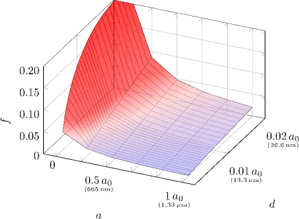
Figure 9: Fractional difference in the Lifshitz energy $E(a,b)$ per surface area $4\pi a^{2}$ of the inner sphere of radius $a$ of a shell of water of thickness $d$ engulfing an ice ball of radius $a$, with respect to the Lifshitz energy per unit area ${\cal E}$ for a planar geometry, plotted as a function of $a$ and $d$. The fractional error $f=1-\frac{E(a,b)}{4\pi a^{2}}\frac{1}{{\cal E}}$ is plotted. The plots verify the general understanding that the Lifshitz energy per unit area for a spherical configuration approaches that of a planar configuration for small thickness $d$.

It is often convenient to approximate the Lifshitz energy for the configuration of concentric spheres with the corresponding Lifshitz energy for planar configuration scaled with a suitable area. This is often called the proximity force approximation, and is usually a good approximation when the thickness of the intermediate medium is small compared to the radii of the inner and outer spheres. In Fig. 9 we plot the fractional error in using this approximation. This error is small for large radii of ice and small thickness of water, and the error gets significant for small radii of ice and large thickness of water layer.

VII Conclusion and outlook

In this article, we successfully demonstrated that the Lifshitz energy for concentric spherical configurations in Fig. 4 can be computed with relative ease. As an application we considered the case of solid ice enclosed by liquid water inside water vapor at the triple point of water, and thereby extended the analysis of Elbaum and Schick in Ref. Elbaum and Schick (1991a) to spherical interfaces. Our study shows that a drop of water surrounded by vapor, with no ice inside the water, is unstable, and quantum fluctuations promote formation of ice in the drop of water at the triple point of water. It is energetically favorable for the ice to grow indefinitely inside the drop of water while a 3.6 nm thick layer of water encircles the ball of ice. These conclusions ignore self-energies of the interior and exterior spherical regions, which are not uniquely defined. Some of these effects may be subsumed into surface tension, but this omission, unavoidable at this stage of our understanding, renders our conclusions tentative. As noted, the effects we are considering are relatively small compared to nucleation and surface tension effects.

In a following paper we will investigate the configuration of water inside ice inside vapor. That is, is it energetically favorable for ice to form at the interface of water and vapor, and once formed will it grow inwards? This is of interest because in Ref. Elbaum and Schick (1991b) it was found that no ice is formed on a planar water surface based on Lifshitz theory. This is expected to hold for water drops of large radii. In addition, now, we have in the present work found, surprisingly, that purely quantum fluctuations promote freezing from within water droplets instead of freezing from outside.

As an application of the results found here, that ice grows inside water at the triple point of water, we would like to investigate the relevance of this effect to the predictions for liquid water on distant planets and their moons. In presence of a silica surface we have predicted that ice can form in water based on Lifshitz theory Boström et al. (2017). Boström et al. further proposed that Lifshitz forces could lead to ice formation on some specific gas hydrate surfaces in water Boström et al. (2019). On some hypothesized ice coated oceans on the moons Enceladus and Europa such ice films growing on CO₂ gas hydrate clusters could, if present, induce a size dependent buoyancy for nanosized hydrate clusters Boström et al. (2019).

Understanding the charging process of atmospheric ice particles Sherwood et al. (2006) is expected to be a relevant application of the results here. Another application will involve studying ice formation in pores, especially inside rocks and plants, in light of our results here. In some situations double layer interaction energy be significant in comparison to the Lifshitz energy as was discussed in Ref. Thiyam et al. (2018b), which could be extended to the spherical geometry.

*

Appendix A Lifshitz interaction energy for concentric spheres

In this appendix we use $\hbar=1$ and $c=1$ for typographic brevity. This can be undone by replacing $\zeta\to\zeta/c$ and introducing $\hbar$ in equations for energy.

In the multiple scattering formalism the Lifshitz interaction energy for the configuration of concentric spheres in Fig. 4 is given by

$$E_{12}(a,b)=\frac{1}{2}\int_{-\infty}^{\infty}\frac{d\zeta}{2\pi}\,\text{Tr}\,\ln\Big{[}{\bf 1}-{\bm{\Gamma}}_{a}V_{a}\cdot{\bm{\Gamma}}_{b}V_{b}\Big{]},$$ (29)

where

$$V_{a} = (\varepsilon_{3}-1)+(\varepsilon_{1}-\varepsilon_{3})\theta(a-r),$$ (30a)

$$V_{b} = (\varepsilon_{3}-1)+(\varepsilon_{2}-\varepsilon_{3})\theta(r-b),$$ (30b)

each, describe concentric spherical regions with a single interface, obtained by letting $b\to\infty$ and $a\to 0$, respectively, in Fig. 4. The interaction energy of Eq. (29) corresponds to the fourth term in the decomposition of energy in Eq. (1) for the system in Fig. 4, which is finite by construction. In Eq. (29) we used symbolic notation,

$${\bm{\Gamma}}_{a}V_{a}\cdot{\bm{\Gamma}}_{b}V_{b}=\int d^{3}\bar{r}\,{\bm{\Gamma}}_{a}({\bf r},\bar{\bf r})V_{a}(\bar{\bf r})\cdot{\bm{\Gamma}}_{b}(\bar{\bf r},{\bf r}^{\prime})V_{b}({\bf r}^{\prime}).$$ (31)

Thus, the argument of the logarithm in Eq. (29) is a dyadic, or a matrix, with elements constituting integral kernels. The trace in Eq. (29) is over the matrix indices and on the kernel coordinates ${\bf r}$ and ${\bf r}^{\prime}$. The Green dyadics ${\bm{\Gamma}}_{a}({\bf r},{\bf r}^{\prime})$ and ${\bm{\Gamma}}_{b}({\bf r},{\bf r}^{\prime})$ can be suitably expressed in the basis of spherical vector eigenfunctions Shajesh et al. (2017)

$${\bf X}_{lm}^{(u)}(\theta,\phi) =\frac{1}{ik_{\perp}}{\bm{\nabla}}_{\perp}Y_{lm}(\theta,\phi),$$ (32a)

$${\bf X}_{lm}^{(v)}(\theta,\phi) =\frac{1}{ik_{\perp}}\hat{\bf r}\times{\bm{\nabla}}_{\perp}Y_{lm}(\theta,\phi),$$ (32b)

$${\bf X}_{lm}^{(w)}(\theta,\phi) =\hat{\bf r}\,Y_{lm}(\theta,\phi),$$ (32c)

expressed in terms of spherical harmonics $Y_{lm}(\theta,\phi)$, as

$${\bm{\Gamma}}_{\alpha}({\bf r},{\bf r}^{\prime})=\hskip 170.71652pt$$

$$\hskip 14.22636pt\sum_{l=0/1}^{\infty}\sum_{m=-l}^{l}{\bf X}_{lm}^{(i)}(\theta,\phi)\gamma_{lm,\alpha}^{ij}(r,r^{\prime}){\bf X}_{lm}^{(j)*}(\theta^{\prime},\phi^{\prime}),\hskip 22.76219pt$$ (33)

$\alpha=a,b$, where $0/1$ for the initial value of index $l$ means that the sum over $l$ runs from 0 to $\infty$ for terms involving ${\bf X}_{lm}^{(w)}$, but $l$ runs from 1 to $\infty$ for terms involving ${\bf X}_{lm}^{(u)}$ and ${\bf X}_{lm}^{(v)}$. The matrices $\gamma_{lm,\alpha}^{ij}(r,r^{\prime})$ are the components of the Green dyadics in the basis of spherical vector eigenfunctions given by

$$\gamma_{lm,\alpha}^{ij}(r,r^{\prime})=\hskip 170.71652pt$$

$$\left[\begin{array}[]{c}\frac{D}{\varepsilon_{\alpha}(r)}\frac{D^{\prime}}{\varepsilon_{\alpha}(r^{\prime})}g_{l,\alpha}^{H}(r,r^{\prime})\hskip 8.53581pt0\hskip 8.53581pt\frac{D}{\varepsilon_{\alpha}(r)}\frac{ik_{\perp}^{\prime}}{\varepsilon_{\alpha}(r^{\prime})}g_{l,\alpha}^{H}(r,r^{\prime})\\[5.69054pt] 0\hskip 28.45274pt-\zeta^{2}g_{l,\alpha}^{E}(r,r^{\prime})\hskip 28.45274pt0\\[5.69054pt] \frac{-ik_{\perp}}{\varepsilon_{\alpha}(r)}\frac{D^{\prime}}{\varepsilon_{\alpha}(r^{\prime})}g_{l,\alpha}^{H}(r,r^{\prime})\hskip 8.53581pt0\hskip 8.53581pt\frac{-ik_{\perp}}{\varepsilon_{\alpha}(r)}\frac{ik_{\perp}^{\prime}}{\varepsilon_{\alpha}(r^{\prime})}g_{l,\alpha}^{H}(r,r^{\prime})\end{array}\right],\hskip 22.76219pt$$ (37)

where

$$\varepsilon_{a}(r)=\begin{cases}\varepsilon_{1},&r<a,\\ \varepsilon_{3},&a<r,\end{cases}$$ (38)

and

$$\varepsilon_{b}(r)=\begin{cases}\varepsilon_{3},&r<b,\\ \varepsilon_{2},&b<r,\end{cases}$$ (39)

with shorthand notations

$$k_{\perp}^{2}=\frac{l(l+1)}{r^{2}},\qquad k_{\perp}^{\prime\,2}=\frac{l(l+1)}{{r^{\prime}}^{2}},$$ (40)

and

$$D=\left(\frac{1}{r}+\frac{\partial}{\partial r}\right)=\frac{1}{r}\frac{\partial}{\partial r}r$$ (41)

and similarly for $D^{\prime}$ with primed coordinates. We have omitted a term containing a $\delta$-function in Eq. (37), which does not contribute to interaction energies between disjoint bodies. The transverse magnetic and transverse electric spherical Green’s functions in Eq. (37) satisfy the differential equations

$$\left[-D\frac{1}{\varepsilon_{\alpha}(r)}D+\frac{l(l+1)}{r^{2}\varepsilon_{\alpha}(r)}+\zeta^{2}\right]g_{l,\alpha}^{H}(r,r^{\prime}) = \frac{\delta(r-r^{\prime})}{r^{2}},$$ (42a)

$$\left[-D^{2}+\frac{l(l+1)}{r^{2}}+\zeta^{2}\varepsilon_{\alpha}(r)\right]g_{l,\alpha}^{E}(r,r^{\prime}) = \frac{\delta(r-r^{\prime})}{r^{2}},\hskip 39.83385pt$$ (42b)

$\alpha=a,b$, and have solutions

$$g_{l,a}^{H}(r^{\prime},r) = -\frac{\varepsilon_{1}}{a}\frac{1}{(\zeta_{1}a)}\frac{\zeta_{3}\,\text{i}_{l}(\zeta_{1}r)\text{k}_{l}(\zeta_{3}r^{\prime})}{\left[\zeta_{1}\,\text{i}_{l}(\zeta_{1}a)\bar{\text{k}}_{l}(\zeta_{3}a)-\zeta_{3}\,\bar{\text{i}}_{l}(\zeta_{1}a)\text{k}_{l}(\zeta_{3}a)\right]},$$ (43a)

$$g_{l,b}^{H}(r,r^{\prime}) = -\frac{\varepsilon_{2}}{b}\frac{1}{(\zeta_{2}b)}\frac{\zeta_{3}\,\text{i}_{l}(\zeta_{3}r)\text{k}_{l}(\zeta_{2}r^{\prime})}{\left[\zeta_{3}\,\text{i}_{l}(\zeta_{3}b)\bar{\text{k}}_{l}(\zeta_{2}b)-\zeta_{2}\,\bar{\text{i}}_{l}(\zeta_{3}b)\text{k}_{l}(\zeta_{2}b)\right]},$$ (43b)

$$g_{l,a}^{E}(r^{\prime},r) = -\frac{1}{a}\frac{1}{(\zeta_{1}a)}\frac{\zeta_{1}\,\text{i}_{l}(\zeta_{1}r)\text{k}_{l}(\zeta_{3}r^{\prime})}{\left[\zeta_{3}\,\text{i}_{l}(\zeta_{1}a)\bar{\text{k}}_{l}(\zeta_{3}a)-\zeta_{1}\,\bar{\text{i}}_{l}(\zeta_{1}a)\text{k}_{l}(\zeta_{3}a)\right]},$$ (43c)

$$g_{l,b}^{E}(r,r^{\prime}) = -\frac{1}{b}\frac{1}{(\zeta_{2}b)}\frac{\zeta_{2}\,\text{i}_{l}(\zeta_{3}r)\text{k}_{l}(\zeta_{2}r^{\prime})}{\left[\zeta_{2}\,\text{i}_{l}(\zeta_{3}b)\bar{\text{k}}_{l}(\zeta_{2}b)-\zeta_{3}\,\bar{\text{i}}_{l}(\zeta_{3}b)\text{k}_{l}(\zeta_{2}b)\right]},\hskip 14.22636pt$$ (43d)

in terms of modified spherical Bessel functions of Eqs. (16) and generalized derivatives of of modified spherical Bessel functions in Eqs. (17) with

$$\zeta_{i}=\zeta\sqrt{\varepsilon_{i}}.$$ (44)

To evaluate the Lifshitz interaction energy we begin by processing the dyadic in Eq. (31). We use the expressions for the Green dyadics in Eq. (33) and using the orthogonality relations for the spherical vector eigenfunctions,

$$\int_{0}^{\pi}\sin\theta d\theta\int_{0}^{2\pi}d\phi\,{\bf X}_{lm}^{*(i)}(\theta,\phi){\bf X}_{l^{\prime}m^{\prime}}^{(j)}(\theta,\phi)\hskip 42.67912pt$$

$$=\delta_{ll^{\prime}}\delta_{mm^{\prime}}\delta_{ij},\hskip 142.26378pt$$ (45)

for the angular part of coordinate $\bar{\bf r}$, we obtain

$${\bm{\Gamma}}_{a}V_{a}\cdot{\bm{\Gamma}}_{b}V_{b}=\sum_{l=0}^{\infty}\sum_{m=-l}^{l}{\bf X}_{lm}^{(i)}(\theta,\phi){\bf X}_{lm}^{*(k)}(\theta^{\prime},\phi^{\prime})\hskip 28.45274pt$$

$$\times\int\bar{r}^{2}d\bar{r}\,\gamma_{lm,a}^{ij}(r,\bar{r})V_{a}(\bar{r})\gamma_{lm,b}^{jk}(\bar{r},r^{\prime})V_{b}(r^{\prime}).\hskip 28.45274pt$$ (46)

We observe the separation of the angular coordinates in this form, which is attributable to the spherical symmetry of the configuration of concentric sphere geometry. Using this feature as a cornerstone, we expand the logarithm as a series. In each term of the series the angular terms separate after repeated use of orthogonality relations for the spherical vector eigenfunctions. This allows for the separation of the angular coordinates completely and in conjunction with the trace in the equation the angular coordinates drop out of the equation, leaving a sum over $l$ and a factor of $(2l+1)$ from the sum over $m$. The leftover series involves integrals in radial coordinates, which, remarkably, allows for the series to be resummed. These manipulations, which are mostly formal rearrangement of integrals, are crucial part of the calculation and leads to the expression

$$E_{12}(a,b) = \frac{1}{2}\int_{-\infty}^{\infty}\frac{d\zeta}{2\pi}\sum_{l=0}^{\infty}(2l+1)$$ (47)

$$\times\ln\big{[}1-K_{l}^{E}(a,b)\big{]}\big{[}1-K_{l}^{H}(a,b)\big{]},\hskip 14.22636pt$$

where

$$K_{l}^{E}(a,b) = \zeta^{2}(\varepsilon_{1}-\varepsilon_{3})(\varepsilon_{2}-\varepsilon_{3})\int_{0}^{a}r^{2}dr\int_{b}^{\infty}{r^{\prime}}^{2}dr^{\prime}$$ (48)

$$\times g_{l,a}^{E}(r^{\prime},r)g_{l,b}^{E}(r,r^{\prime})\hskip 14.22636pt$$

and

$$K_{l}^{H}(a,b)=\left(\frac{1}{\varepsilon_{3}}-\frac{1}{\varepsilon_{1}}\right)\left(\frac{1}{\varepsilon_{3}}-\frac{1}{\varepsilon_{2}}\right)\int_{0}^{a}r^{2}dr\int_{b}^{\infty}{r^{\prime}}^{2}dr^{\prime}$$

$$\times\text{tr}\left[\begin{array}[]{cc}D^{\prime}Dg_{l,a}^{H}(r^{\prime},r)&D^{\prime}ik_{\perp}g_{l,a}^{H}(r^{\prime},r)\\ -ik_{\perp}^{\prime}Dg_{l,a}^{H}(r^{\prime},r)&k_{\perp}k_{\perp}^{\prime}g_{l,a}^{H}(r^{\prime},r)\end{array}\right]\hskip 28.45274pt$$ (51)

$$\times\left[\begin{array}[]{cc}D^{\prime}Dg_{l,b}^{H}(r,r^{\prime})&D^{\prime}ik_{\perp}g_{l,b}^{H}(r,r^{\prime})\\ -ik_{\perp}^{\prime}Dg_{l,b}^{H}(r,r^{\prime})&k_{\perp}k_{\perp}^{\prime}g_{l,b}^{H}(r,r^{\prime})\end{array}\right].\hskip 28.45274pt$$ (54)

The integration limits on the coordinate $r$ spans the inner spherical region from 0 to $a$, and the integration limits on the radial coordinate $r^{\prime}$ spans the outer spherical region beyond $b$, and, together, they span disjoint regions in space. This segregation of variables avoids ultraviolet divergences in the energy associated with $r\to r^{\prime}$.

Evaluating the expression in Eq. (48) after substituting the solutions for Green’s functions from Eqs. (43) we observe the factorization

$$K_{l}^{E}(a,b)=r_{31}^{E}(a)r_{32}^{E}(b),$$ (55)

where $r_{ij}^{E}$ are the scattering coefficients for the transverse electric mode of an electromagnetic wave incident on interfaces $a$ or $b$. The transverse electric scattering coefficients at the two interfaces can be expressed in the form

$$r_{31}^{E}(a) = \frac{1}{a^{2}}\frac{(\zeta_{1}^{2}-\zeta_{3}^{2})\int_{0}^{a}r^{2}dr\,\text{i}_{l}(\zeta_{1}r)\text{i}_{l}(\zeta_{3}r)}{\left[\zeta_{3}\,\text{i}_{l}(\zeta_{1}a)\bar{\text{k}}_{l}(\zeta_{3}a)-\zeta_{1}\,\bar{\text{i}}_{l}(\zeta_{1}a)\text{k}_{l}(\zeta_{3}a)\right]},$$ (56a)

$$r_{32}^{E}(b) = \frac{1}{b^{2}}\frac{(\zeta_{2}^{2}-\zeta_{3}^{2})\int_{b}^{\infty}r^{2}dr\,\text{k}_{l}(\zeta_{2}r)\text{k}_{l}(\zeta_{3}r)}{\left[\zeta_{2}\,\text{i}_{l}(\zeta_{2}b)\bar{\text{k}}_{l}(\zeta_{2}b)-\zeta_{3}\,\bar{\text{i}}_{l}(\zeta_{3}b)\text{k}_{l}(\zeta_{3}b)\right]}.\hskip 36.98857pt$$ (56b)

The integrals appearing in the numerators of the transverse electric scattering coefficients can be evaluated using the identities Prudnikov et al. (1990); Inc.

$$\int_{0}^{x}y^{2}dy\,\text{i}_{l}(py)\text{i}_{l}(qy)\hskip 156.49014pt$$

$$\hskip 14.22636pt=-\frac{x^{2}}{(p^{2}-q^{2})}\Big{[}q\text{i}_{l}(px)\bar{\text{i}}_{l}(qx)-p\bar{\text{i}}_{l}(px)\text{i}_{l}(qx)\Big{]},\hskip 34.1433pt$$ (57a)

$$\int_{x}^{\infty}y^{2}dy\,\text{k}_{l}(py)\text{k}_{l}(qy)\hskip 147.95433pt$$

$$\hskip 14.22636pt=\frac{x^{2}}{(p^{2}-q^{2})}\Big{[}q\text{k}_{l}(px)\bar{\text{k}}_{l}(qx)-p\bar{\text{k}}_{l}(px)\text{k}_{l}(qx)\Big{]},\hskip 34.1433pt$$ (57b)

which immediately leads to the expression for the transverse electric scattering coefficients in Eqs. (14). The contribution from the transverse magnetic mode can be similarly factorized into

$$K_{l}^{H}(a,b)=r_{31}^{H}(a)r_{32}^{H}(b),$$ (58)

where $r_{ij}^{H}$ are the scattering coefficients for the transverse magnetic mode of an electromagnetic wave incident on interfaces $a$ or $b$. The transverse magnetic scattering coefficients can be expressed as

$$r_{31}^{H}(a)=\frac{1}{a^{2}}(\zeta_{1}^{2}-\zeta_{3}^{2})\hskip 156.49014pt$$

$$\times\frac{\int_{0}^{a}r^{2}dr\,\left[\bar{\text{i}}_{l}(\zeta_{1}r)\bar{\text{i}}_{l}(\zeta_{3}r)+\frac{l(l+1)}{r^{2}\zeta_{1}\zeta_{3}}\text{i}_{l}(\zeta_{1}r)\text{i}_{l}(\zeta_{3}r)\right]}{\left[\zeta_{1}\,\text{i}_{l}(\zeta_{1}a)\bar{\text{k}}_{l}(\zeta_{3}a)-\zeta_{3}\,\bar{\text{i}}_{l}(\zeta_{1}a)\text{k}_{l}(\zeta_{3}a)\right]},\hskip 34.1433pt$$ (59a)

$$r_{32}^{H}(b)=\frac{1}{b^{2}}(\zeta_{2}^{2}-\zeta_{3}^{2})\hskip 159.33542pt$$

$$\times\frac{\int_{b}^{\infty}r^{2}dr\,\left[\bar{\text{k}}_{l}(\zeta_{2}r)\bar{\text{k}}_{l}(\zeta_{3}r)+\frac{l(l+1)}{r^{2}\zeta_{2}\zeta_{3}}\text{k}_{l}(\zeta_{2}r)\text{k}_{l}(\zeta_{3}r)\right]}{\left[\zeta_{3}\,\text{i}_{l}(\zeta_{3}a)\bar{\text{k}}_{l}(\zeta_{2}a)-\zeta_{2}\,\bar{\text{i}}_{l}(\zeta_{3}a)\text{k}_{l}(\zeta_{2}a)\right]},\hskip 34.1433pt$$ (59b)

where the integrals appearing in the numerators can be evaluated using the identities Prudnikov et al. (1990); Inc.

$$\int_{0}^{x}y^{2}dy\,\left[\bar{\text{i}}_{l}(py)\bar{\text{i}}_{l}(qy)+\frac{l(l+1)}{y^{2}pq}\text{i}_{l}(py)\text{i}_{l}(qy)\right]\hskip 56.9055pt$$

$$\hskip 8.53581pt=\frac{x^{2}}{(p^{2}-q^{2})}\Big{[}p\text{i}_{l}(px)\bar{\text{i}}_{l}(qx)-q\bar{\text{i}}_{l}(px)\text{i}_{l}(qx)\Big{]},\hskip 48.36967pt$$ (60a)

$$\int_{x}^{\infty}y^{2}dy\,\left[\bar{\text{k}}_{l}(py)\bar{\text{k}}_{l}(qy)+\frac{l(l+1)}{y^{2}pq}\text{k}_{l}(py)\text{k}_{l}(qy)\right]\hskip 42.67912pt$$

$$\hskip 8.53581pt=-\frac{x^{2}}{(p^{2}-q^{2})}\Big{[}p\text{k}_{l}(px)\bar{\text{k}}_{l}(qx)-q\bar{\text{k}}_{l}(px)\text{k}_{l}(qx)\Big{]},\hskip 34.1433pt$$ (60b)

which leads leads to the expression for the transverse magnetic scattering coefficients in Eqs. (14). Thus, we obtain the expression for the Lizshitz interaction energy in terms of scattering coefficients to be

$$E_{12}(a,b)=\frac{1}{2}\int_{-\infty}^{\infty}\frac{d\zeta}{2\pi}\sum_{l=0}^{\infty}(2l+1)\hskip 71.13188pt$$

$$\times\ln\big{[}1-r_{31}^{E}(a)r_{32}^{E}(b)\big{]}\big{[}1-r_{31}^{H}(a)r_{32}^{H}(b)\big{]}.\hskip 14.22636pt$$ (61)

This expression for Lifshitz interaction energy is for zero temperature. The interaction energy for nonzero temperature in Eq. (13) is obtained from the above expression by the replacement

$$\frac{1}{2}\int_{-\infty}^{\infty}\frac{d\zeta}{2\pi}\to\frac{\hbar c}{2\pi a_{0}}{\sum_{n=0}^{\infty}}{{}^{\prime}}.$$ (62)