Abstract

Our goal is the discussion of the problem of mathematical interpretation of basic postulates (or ‘principles’) of Quantum Mechanics: transitions to quantum stationary orbits, the wave-particle duality, and the probabilistic interpretation, in the context of semiclassical self-consistent Maxwell–Schrödinger equations. We discuss possible relations of these postulates to the theory of attractors of Hamiltonian nonlinear PDEs relying on a new general mathematical conjecture on global attractors of G-invariant nonlinear Hamiltonian partial differential equations with a Lie symmetry group G.

This conjecture is inspired by our results on global attractors of nonlinear Hamiltonian PDEs obtained since 1990 for a list of model equations with three basic symmetry groups: the trivial group, the group of translations, and the unitary group U(1). We present sketchy these results.

To Sasha Shnirelman on occasion of his 75-th anniversary

Keywords: attractors; stationary states; solitons; stationary orbits; Hamiltonian equations; nonlinear partial differential equations; symmetry group; Lie group; Lie algebra; Maxwell–Schrödinger equations;  quantum transitions; wave-particle duality; electron diffraction; probabilistic interpretation.

1 Quantum postulates and Maxwell–Schrödinger equations

The present paper is inspired by the problem of a mathematical description of ‘quantum jumps’, i.e., of transitions between quantum stationary orbits. We discuss the problem of mathematical description of basic postulates of quantum theory:

A. Transitions between quantum stationary orbits (N. Bohr, 1913).

B. Wave-particle duality (L. de Broglie, 1923).

C. Probabilistic interpretation (M. Born, 1927).  
The problem concerns the validity of these postulates in Schrödinger’s quantum mechanics, and it still remains an open problem. These and other questions have been frequently addressed in the 1920s and 1930s in hot discussions by Bohr, Schrödinger, Einstein and others [1]. However, a satisfactory solutions were not achieved, and a rigorous dynamical description of these postulates is still unknown. This lack of theoretical clarity hinders the progress in the theory (e.g., in superconductivity and in nuclear reactions), and in numerical simulation of many engineering processes (e.g., of laser radiation and quantum amplifiers) since a computer can solve dynamical equations, but cannot take into account postulates.

We discuss the possible relations of these postulates to the theory of attractors of Hamiltonian nonlinear PDEs in the context of semiclassical self-consistent Maxwell–Schrödinger equations (MS), applying a novel general mathematical conjecture on global attractors of G-invariant nonlinear Hamiltonian partial differential equations with a Lie symmetry group G.

This conjecture was inspired by a number of results on global attractors of nonlinear Hamiltonian PDEs obtained since 1990 for a list of model equations with three basic symmetry groups: the trivial group, the group of translations, and the unitary group U(1). We briefly present these results. However, for the Maxwell–Schrödinger equations, the justification of global attraction still remains an open problem.

Note that the second-quantized MS system is the main subject of Quantum Electrodynamics [5]. Our specific attention to the semiclassical MS equations is due to the fact that for this system an extensive empirical material is available: on atomic spectra, electron diffraction, on crystals and their thermal and electric conductivity, etc. Therefore, one can try to find a possible mathematical description of these phenomena in the framework of the MS system and try to prove it. So the MS system serves as a testing ground for the development of the theory. The same questions are open in Quantum Field Theory.  However, these questions obviously cannot be clarified until they are understood in the simpler context of semiclassical theory.

The coupled Maxwell–Schrödinger equations in the Coulomb gauge ${\rm div{\hskip 1.42262pt}}{\bf A}(x,t)\equiv 0$ read as (cf. [5, 16])

$$\!\!\!\!\!\!\left\{\begin{array}[]{rcl}\frac{1}{c^{2}}\ddot{\bf A}(x,t)\!\!\!&\!\!=\!\!&\!\!\!\Delta{\bf A}(x,t)+\frac{1}{c}P{\bf j}(x,t),\quad\Delta A^{0}(x,t)=-\rho(x,t)\\ \\ ~i\hbar\dot{\psi}(x,t)\!\!\!&\!\!=\!\!&\!\!\!\frac{1}{2{\rm m}}[-i\hbar\nabla\!-\!\displaystyle\frac{e}{c}({\bf A}(x,t)\!+\!{\bf A}_{\rm ext}(x,t))]^{2}\psi(x,t)\!+\!e(A^{0}(x,t)\!+\!A^{0}_{\rm ext}(x,t))\psi(x,t)\end{array}\right|\,x\in{\mathbb{R}}^{3},$$ (1.1)

where ${\bf A}_{\rm ext}(x,t)$ and $A^{0}_{\rm ext}(x,t)$ are external Maxwell potentials, $e<0$ is the electron charge and $c$ is the speed of light in a vacuum. The coupling is completed by expressing the charge and current densities in the wave function:

$$\rho(x,t)=e|\psi(x,t)|^{2},\qquad{\bf j}(x,t)=\frac{e}{{\rm m}}{\rm Re{\hskip 1.42262pt}}\{\overline{\psi}(x,t)[-i\hbar\nabla-\frac{e}{c}({\bf A}(x,t)+{\bf A}_{\rm ext}(x,t))]\psi(x,t)\}.$$ (1.2)

These densities satisfy the continuity identity $\dot{\rho}(x,t)+{\rm div{\hskip 1.42262pt}}{\bf j}(x,t)\equiv 0.$ The system (1.1) is formally Hamiltonian, with the Hamiltonian functional (which is the energy up to a factor)

$${\cal H}(\bm{\Pi},{\bf A},\psi,t)=\frac{1}{2}[\|\frac{1}{c}\bm{\Pi}\|^{2}+\|{\rm rot{\hskip 1.42262pt}}{\bf A}\|^{2}]+(\psi,H({\bf A},\psi,t)\psi),$$ (1.3)

where $\|\cdot\|$ stands for the norm in the real Hilbert space $L^{2}({\mathbb{R}}^{3})\otimes{\mathbb{R}}^{3}$ and the brackets $(\cdot,\cdot)$ stand for the inner product in $L^{2}({\mathbb{R}}^{3})\otimes{\mathbb{C}}$. The Schrödinger operator is defined by

$$H({\bf A},\psi,t):=\frac{1}{2m}[-i\hbar\nabla-\displaystyle\frac{e}{c}({\bf A}(x)+{\bf A}_{\rm ext}(x,t))]^{2}+e(\frac{1}{2}A^{0}(x)+A^{0}_{\rm ext}(x,t)),$$

where $A^{0}(x):=(-\Delta)^{-1}\rho$ with $\rho(x):=e|\psi(x)|^{2}$. The system (1.1) can be written in the Hamiltonian form with variational derivatives as

$$\left\{\begin{array}[]{l}\frac{1}{c^{2}}\dot{\bf A}(t)=D_{\bm{\Pi}}{\cal H}(\bm{\Pi(t)},{\bf A}(t),\psi(t),t),\,\qquad\frac{1}{c^{2}}\dot{\bm{\Pi}}(t)=-D_{\bf A}{\cal H}(\bm{\Pi}(t),{\bf A}(t),\psi(t),t)\vskip 6.0pt plus 2.0pt minus 2.0pt\\ i\hbar\dot{\psi}(t)=\frac{1}{2}D_{\psi}{\cal H}(\bm{\Pi}(t),{\bf A}(t),\psi(t),t)=H({\bf A}(t),\psi(t),t)\psi(t),\end{array}\right|,$$ (1.4)

taking into account that $(\psi,eA^{0}\psi)=(A^{0},\rho)=((-\Delta)^{-1}\rho,\rho)$, and hence, $D_{\psi}(\psi,eA^{0}\psi)=4eA^{0}\psi$. Therefore, the energy is conserved in the case of static external potentials

$${\bf A}_{\rm ext}(x,t)\equiv{\bf A}_{\rm ext}(x),\qquad A^{0}_{\rm ext}(x,t)\equiv A^{0}_{\rm ext}(x).$$ (1.5)

For instance, in the case of an atom, $A^{0}_{\rm ext}(x)$ is the Coulomb potential of the nucleus, while ${\bf A}_{\rm ext}(x)$ is the vector potential of the nucleus magnetic field. The Hamiltonian (1.3) is invariant with respect to the action of the group $U(1)$,

$$({\bf A}(x),\bm{\Pi}(x),\psi(x))\mapsto({\bf A}(x),\bm{\Pi}(x),\psi(x)e^{i\theta}),\qquad\theta\in(0,2\pi).$$ (1.6)

Remark 1.1.

The existence of global solutions to the Cauchy problems for systems (1.1) in the entire space ${\mathbb{R}}^{3}$ without external potentials was proved in [14] for all finite energy initial states (1.3). The uniqueness of solutions in the energy space was proved in [11].

Remark 1.2.

The system (1.1) was essentially introduced by Schrödinger in his first articles [7], and it underlies the entire theory of laser radiation [13].

2 Quantum jumps and attractors

In 1913, Bohr formulated the following two fundamental postulates of the quantum theory of atoms:
I. An atom always lives in one of the quantum stationary orbits, and sometimes it jumps from one stationary state to another: in the Dirac notation

$$|E_{n}\rangle\mapsto|E_{n^{\prime}}\rangle.$$ (2.1)

II. The atom does not radiate in stationary orbits. Every jump is followed by a radiation of an electromagnetic wave with the frequency

$$~\omega_{nn^{\prime}}=\frac{E_{n^{\prime}}-E_{n}}{\hbar}=\omega_{n^{\prime}}-\omega_{n},\qquad\omega_{n}:=E_{n}/\hbar,$$ (2.2)

Both these postulates were inspired i) by stability of atoms and ii) by the Rydberg–Ritz Combination Principle. With the discovery of the Schrödinger theory in 1926, the question aroses about the implementation of the above Bohr axioms in the new theory.

2.1 Schrödinger theory of stationary orbits

Besides the equation for the wave function, the Schrödinger theory contains a highly nontrivial definition of stationary orbits (or quantum stationary states) in the case when  the Maxwell external potentials do not depend on time: In this case, the Schrödinger equation reads as

$$i\hbar\dot{\psi}(x,t)=H\psi(t):=\frac{1}{2{\rm m}}[-i\hbar\nabla-\displaystyle\frac{e}{c}{\bf A}_{\rm ext}(x)]^{2}\psi(x,t)+eA_{\rm ext}^{0}(x)\psi(x,t).$$ (2.3)

The corresponding stationary orbits are defined as finite-energy solutions of the form

$$\psi(x,t)\equiv\psi(x)e^{-i\omega t},\qquad\omega\in{\mathbb{R}}.$$ (2.4)

Substitution into the Schrödinger equation (2.3) leads to the famous eigenvalue problem.

Such definition is rather natural, since then $|\psi(x,t)|$ does not depend on time. Most likely, this definition was suggested by the de Broglie wave function for free particles $\psi(x,t)=Ce^{i(kx-\omega t)}$, which factorises as $Ce^{ikx}e^{-i\omega t}$. Indeed, in the case of bound particles, it is natural to change the spatial factor $Ce^{ikx}$, since the spatial properties have changed and ceased to be homogeneous. On the other hand, the homogeneous time factor $e^{-i\omega t}$ must be preserved, since the external potentials are independent of time. However, these ‘algebraic’ arguments do not withdraw the question on agreement of the Schrödinger definition with the Bohr postulate (2.1)!

Thus, the problem on the mathematical interpretation of the Bohr postulate (2.1) in the Schrödinger theory arises. One of the simplest interpretation of the jump (2.1) is the long-time asymptotics

$$\psi(x,t)\sim\psi_{\pm}(x)e^{-i\omega_{\pm}t},\qquad t\to\pm\infty,$$ (2.5)

for each finite energy solution,  where  $\omega_{-}=\omega_{n}$ and $\omega_{+}=\omega_{n^{\prime}}$. However, for the linear Schrödinger equation (2.3), such asymptotics are obviously wrong, due to the superposition principle: for example, for solutions of the form $\psi(x,t)\equiv\psi_{1}(x)e^{-i\omega_{1}t}+\psi_{2}(x)e^{-i\omega_{2}t}$ with $\omega_{1}\neq\omega_{2}$. It is exactly this contradiction which shows that the linear Schrödinger equation alone cannot serve as a basis for the theory compatible with the Bohr postulates. Our main conjecture is that these asymptotics are inherent properties of the nonlinear Maxwell–Schrödinger equations (1.1). This conjecture is suggested by the following perturbative arguments.

2.2 Bohr’s postulates by perturbation theory

The remarkable success of the Schrödinger theory was in the explanation of Bohr’s postulates via asymptotics (2.5) by means of perturbation theory applied to the coupled Maxwell–Scrödinger equations (1.1) in the case of static external potentials. Namely, as a first approximation, the fields ${\bf A}(x,t)$ and $A^{0}(x,t)$ in the Schrödinger equation of the system  (1.1) can be neglected, so we obtain the equation (2.3).  For ‘sufficiently good’ external potentials and initial conditions, each finite energy solution can be expanded in eigenfunctions  

$$~\psi(x,t)=\sum_{n}C_{n}\psi_{n}(x)e^{-i\omega_{n}t}+\psi_{c}(x,t),\qquad~\psi_{c}(x,t)=~\int C(\omega)e^{-i\omega t}d\omega,$$ (2.6)

where integration is performed over the continuous spectrum of the Schrödinger operator $H$, and for any $R>0$ we have

$$\int_{|x|<R}|\psi_{c}(x,t)dx\to 0,\quad t\to\pm\infty,$$ (2.7)

see, for example, [10, Theorem 21.1]. The substitution of this expansion into the expression for currents (1.2) gives

$$j(x,t)=\sum_{nn^{\prime}}j_{nn^{\prime}}(x)e^{-i\omega_{nn^{\prime}}t}+c.c.+j_{c}(x,t),$$ (2.8)

where $j_{c}(x,t)$ has a continuous frequency spectrum. Thus, the currents on the right hand side of the Maxwell equation from (1.1) contains, besides the continuous spectrum, only discrete frequencies $\omega_{nn^{\prime}}$. Hence, the discrete spectrum of the corresponding Maxwell field also contains only these frequencies $\omega_{nn^{\prime}}$. This jusitfies the Bohr rule (2.2) in the first order of perturbation theory, since this calculation ignores the back effect of radiation into the atom.

Moreover, these arguments also suggest to treat the jumps (2.1) as the single-frequency asymptotics (2.5) for solutions of the Schrödinger equation coupled to the Maxwell equations.

Indeed, the currents (2.8) on the right of the Maxwell equation from (1.1) produce the radiation when non-zero frequencies $\omega_{nn^{\prime}}$ are present. This is due to the fact that ${\mathbb{R}}\setminus 0$ is the absolutely continuous spectrum of the Maxwell equations.

However, this radiation cannot last forever, since it irrevocably carries the energy to infinity while the total energy is finite. Therefore, in the long-time limit only $\omega_{nn^{\prime}}=0$ survives, which means exactly that we have single-frequency asymptotics (2.5) in view of (2.7).

Remark 2.1.

Of course, these perturbation arguments cannot provide a rigorous justification of the long-time asymptotics (2.5) for the coupled Maxwell–Schrödinger equations. In [50]–[55], we have justified similar single-frequency asymptotics for a list of model nonlinear PDEs with the symmetry group $U(1)$. Nevertheless, for the coupled Maxwell–Schrödinger equation such a justification is still an open problem.

2.3 Bohr’ postulates as global attraction

The perturbation arguments above suggest that the Bohr postulates can be treated as the long-time asymptotics

$$({\bf A}(x,t),\psi(x,t))\sim({\bf A}_{\pm}(x),e^{-i\omega_{\pm}t}\psi_{\pm}(x)),\qquad t\to\pm\infty$$ (2.9)

for all finite-energy solutions of the Maxwell–Schrödinger equations (1.1) in the case of static external potentials (1.5). We conjecture that these asymptotics hold in $H^{1}$-norms on every bounded region of ${\mathbb{R}}^{3}$.

Remark 2.2.

Experiments show that the transition time of quantum jumps (2.1) is of the order $10^{-8}s$, although the asymptotics (2.9) require infinite time. We suppose that this discrepancy can be explained by the following arguments:
i) $10^{-8}$s is the transition time between very small neighborhoods of initial and final states, and
ii) during this time the atom emits an overwhelming part of the radiated energy.

The asymptotics (2.9) have not been proved for the Maxwell–Schrödinger system (1.1). On the other hand, similar asymptotics are now proved for a number of model Hamiltonian nonlinear PDEs with the symmetry group $U(1)$. In next section we state a general conjecture which reduces to the asymptotics (2.9) in the case of the Maxwell–Schrödinger system.

Definition 2.3.

Stationary orbits of the Maxwell–Schrödinger nonlinear system (1.1) are finite energy solutions of the form

$$(A(x),e^{-i\omega t}\psi(x)).$$ (2.10)

The existence of stationary orbits for the system (1.1) was proved in [15] in the case of external potentials

$${\bf A}_{\rm ext}(x,t)\equiv 0,\qquad A_{\rm ext}^{0}(x,t)=-\frac{eZ}{|x|},\qquad\int|\psi_{\pm}(x)|^{2}dx\leq Z.$$ (2.11)

The asymptotics (2.9) mean that a global attraction to the set of stationary orbits occurs. We suggest that a similar attraction takes place for Maxwell–Dirac, Maxwell–Yang–Mills and other coupled equations. In other words, we suggest to interpret quantum stationary states as the points and trajectories that constitute the global attractor of the corresponding quantum dynamical equations.

2.4 The Einstein–Ehrenfest paradox and bifurcation of attractors

An instant orientation of the atomic magnetic moment during $\sim 10^{-4}s$, when turning on the magnetic field in the Stern–Gerlach experiments, led to a discussion in the ‘Old Quantum Mechanics’, because the classical model gave relaxation time $\sim 10^{9}s$, taking into account the moment of inertia of the atom [3]. In the linear Schrödinger’s theory, this phenomenon also did not find a satisfactory explanation.

On the other hand, this instantaneous orientation is exactly in line with asymptotics (2.9) for solutions of the coupled nonlinear Maxwell–Pauli equations, i.e., the Maxwell–Schrödinger system with spin. In the absence of the magnetic field, the minimal eigenvalue is of multiplicity 2, which implies that the manifold of the corresponding ground states $C_{1}\psi_{1}^{0}+C_{2}\psi_{2}^{0}$ with $|C_{1}|^{2}+|C_{2}|^{2}=1$ is of dimension 3. Let us stress that in this case the special role of the states with a fixed spin momenta $s=\pm\frac{1}{2}$ is illusory, since the eigenfuctions depend on the choice of the coordinates in the space ${\mathbb{R}}^{3}$.

However, in a small magnetic field, this minimal eigenvalue bifurcates into two simple eigenvalues. This suggests that for the corresponding nonlinear Maxwell–Pauli equations an instant bifurcation of the global attractor (i.e., of the set of stationary orbits (2.10)) occurs. In particular, new stationary orbits, corresponding to the spin momentum $s=\pm\frac{1}{2}$, appear.

One can expect that the Einstein–Ehrenfest paradox can be explained by a similar bifurcation of the attractor of the coupled nonlinear Maxwell–Pauli system describing the Stern–Gerlach experiment. Indeed, when the magnetic field is turned on, the structure of the attractor instantly changes. Then the trajectory is attracted to a suitable component of new attractor with a certain spin value that corresponds to the ‘alternative A’ in the terminology of Einstein–Ehrenfest [3]: ‘‘… atoms can never fall into the state in which they are quantized not fully". This bifurcation is not related to any rotation of electrons with moment of inertia, which explains the Einstein–Ehrenfest paradox.

2.5 Attractors of dissipative and Hamiltonian PDEs

Such an interpretation of the Bohr transitions as a global attraction is rather natural. On the other hand, the existing theory of attractors of dissipative systems [32]–[35] does not help in this case since all fundamental equations of quantum theory are Hamiltonian. The global attraction for dissipative systems is caused by energy dissipation. However, such a dissipation in the Hamiltonian systems is absent.

This is why the author has developed (in the years 1990–2020), together with his collaborators, a novel theory of global attractors for Hamiltonian PDEs, especially for the application to Quantum Theory problems. All obtained results [37]–[48] for the Hamiltonian equations rely on a thorough analysis of energy radiation, which irrevocably carries the energy to infinity and plays the role of energy dissipation. A brief survey of these results can be found in Section 4, and detailed survey in [55, 56].

The results obtained so far indicate an explicit correspondence between the type of long-time asymptotics of finite energy solutions and the symmetry group of the equations. We formalize this correspondence in our general conjecture (3.5).

3 Conjecture on attractors of $G$-invariant equations

Let us consider general $G$-invariant autonomous Hamiltonian nonlinear PDEs in ${\mathbb{R}}^{n}$ of type

$$\dot{\Psi}(t)=F(\Psi(t)),\qquad t\in{\mathbb{R}},$$ (3.1)

with a Lie symmetry group $G$ acting on a suitable Hilbert or Banach phase space ${\cal E}$ via a linear representation $T$. The Hamiltonian structure means that

$$F(\Psi)=JD{\cal H}(\Psi),\qquad J^{*}=-J,$$ (3.2)

where ${\cal H}$ denotes the corresponding Hamiltonian functional. The $G$-invariance means that

$$F(T(g)\Psi)=T(g)F(\Psi),\qquad\Psi\in{\cal E}$$ (3.3)

for all $g\in G$. In that case, for any solution $\Psi(t)$ of equation (3.1) the trajectory $T(g)\Psi(t)$ is also a solution, so the representation commutes with the dynamical group $U(t):\Psi(0)\mapsto\Psi(t)$,

$$T(g)U(t)=U(t)T(g).$$ (3.4)

Let us note that the theory of elementary particles deals systematically with the symmetry groups $SU(2)$, $SU(3)$, $SU(5)$, $SO(10)$ and others, as well as with the group

$$SU(4)\times SU(2)\times SU(2),$$

which is the symmetry group of ‘Grand Unification’, see [30].
Conjecture A. (On attractors) For ‘generic’ $G$-invariant autonomous equations (3.1), any finite energy solution $\Psi(t)$ admits a long-time asymptotics

$$\Psi(t)\sim e^{\hat{\lambda}_{\pm}t}\Psi_{\pm},\qquad t\to\pm\infty,$$ (3.5)

in the appropriate topology of the phase space ${\cal E}$. Here $\hat{\lambda}_{\pm}=T^{\prime}(e)\lambda_{\pm}$, where $\lambda_{\pm}$ belong to the corresponding Lie algebra $\mathfrak{g}$, while the $\Psi_{\pm}$ are some limiting amplitudes depending on the trajectory $\Psi(t)$ considered.

In other words, all solutions of the type $e^{\hat{\lambda}t}\Psi$ with $\lambda\in\mathfrak{g}$ form a global attractor for generic $G$-invariant Hamiltonian nonlinear PDEs of type (3.1). This conjecture suggests to define stationary $G$-orbits for equation (3.1) as solutions of the type

$$\Psi(t)=e^{\hat{\lambda}t}\Psi,\qquad t\in{\mathbb{R}},$$ (3.6)

where $\lambda$ belongs to the corresponding Lie algebra $\mathfrak{g}$. This definition leads to the corresponding nonlinear eigenvalue problem

$$\hat{\lambda}\Psi=F(\Psi).$$ (3.7)

In particular, for the linear Schrödinger equation with the symmetry group $U(1)$, stationary orbits are solutions of the form $e^{i\omega t}\psi(x)$, where $\omega\in{\mathbb{R}}$ is an eigenvalue of the Schrödinger operator, and $\psi(x)$ is the corresponding eigenfunction. In the case of the symmetry group $G=SU(3)$, the generator (‘eigenvalue’) $\lambda$ is $3\times 3$ -matrix, and solutions (3.6) can be quasiperiodic in time.

Note that the conjecture (3.5) fails for linear equations, i.e., linear equations are exceptional, not ‘generic’!

Empirical evidence. Conjecture (3.5) agrees with the Gell-Mann–Ne’eman theory of baryons [28, 29]. Indeed, in 1961 Gell-Mann and Ne’eman suggested using the symmetry group $SU(3)$ for the strong interaction of baryons relying on the discovered parallelism between empirical data for the baryons, and the ‘‘Dynkin scheme’’ of Lie algebra $\mathfrak{g}=su(3)$ with $8$ generators (the famous ‘eightfold way’). This theory resulted in the scheme of quarks in quantum chromodynamics [30], and in the prediction of a new baryon with prescribed values of its mass and decay products. This particle (the $\Omega^{-}$-hyperon) was promptly discovered experimentally [31].

On the other hand, the elementary particles seem to describe long-time asymptotics of quantum fields. Hence the empirical correspondence between elementary particles and generators of the Lie algebras presumably gives an evidence in favour of our general conjecture (3.5) for equations with Lie symmetry groups.

4 Results on global attractors for nonlinear Hamiltonian PDEs

Here we give a brief survey of rigorous results [37] - [48] obtained since 1990 that confirm conjecture (3.5) for a list of model equations of type (3.1). The details can be found in [55, 56].

The results confirm the existence of finite-dimensional attractors in the Hilbert or Banach phase spaces, and demonstrate an explicit correspondence between the long-time asymptotics and the symmetry group $G$ of equations. The results obtained so far concern equations (3.1) with the following four basic groups of symmetry: the trivial symmetry group $G=\{e\}$, the translation group $G={\mathbb{R}}^{n}$ for translation-invariant equations, the unitary group $G=U(1)$ for phase-invariant equations, and the orthogonal group $SO(3)$ for ‘isotropic’ equations. In these cases, the asymptotics (3.5) reads as follows.  
I. Equations with trivial symmetry group $G=\{e\}$. For such generic equations the conjecture (3.5) means global attraction to stationary states

$$\psi(x,t)\to S_{\pm}(x),\qquad t\to\pm\infty,$$ (4.1)

as illustrated in Fig. 1.

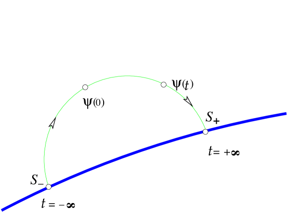
Figure 1: Convergence to stationary states.

Here the states $S_{\pm}=S_{\pm}(x)$ depend on the trajectory $\Psi(t)$ under consideration, and the convergence holds in local seminorms of type $L^{2}(|x|<R)$ with any $R>0$. This convergence cannot hold in global norms (i.e., in norms corresponding to $R=\infty$) due to energy conservation. The asymptotics (4.1) can be symbolically written as the transitions

$$S_{-}\mapsto S_{+},$$ (4.2)

which can be considered as the mathematical model of the Bohr ‘quantum jumps’ (2.1).

Such an attraction was proved for a variety of model equations in [36]–[59]: i) for a string coupled to nonlinear oscillators, ii) for a three-dimensional wave equation coupled to a charged particle and for the Maxwell–Lorentz equations, and also iii) for wave equation, and Dirac and Klein–Gordon equations with concentrated nonlinearities. All proofs rely on the analysis of radiation which irreversibly carries energy to infinity. The details can be found in the survey [56].

In all the problems considered, the convergence (4.1) implies, by the Fatou theorem, the inequality

$${\cal H}(S_{\pm})\leq{\cal H}(Y(t))\equiv{\rm const},\,\,\,t\in{\mathbb{R}},$$ (4.3)

where ${\cal H}$ is the corresponding Hamiltonian (energy) functional. This inequality is an analog of the well known property of weak convergence in Hilbert and Banach spaces. Simple examples show that the strict inequality in (4.3) is possible, which means that an irreversible scattering of energy to infinity occurs.

Example 4.1.

The d’Alembert waves. In particular, the asymptotics (4.1) with the strict inequality (4.3) can easily be demonstrated for the d’Alembert equation $\ddot{\psi}(x,t)=\psi^{\prime\prime}(x,t)$ with general solution

$$\psi(x,t)=f(x-t)+g(x+t).$$ (4.4)

Indeed, the convergence $\psi(\cdot,t)\to 0$ in $L^{2}_{\rm loc}({\mathbb{R}})$ obviously holds for all $f,g\in L^{2}({\mathbb{R}})$. On the other hand, the convergence to zero in global norms obviously fails if $f(x)\not\equiv 0$ or $g(x)\not\equiv 0$.

Example 4.2.

Nonlinear Huygens Principle. Consider solutions of 3D wave equation with a unit propagation velocity and initial data with support in a ball $|x|<R$. The corresponding solution is concentrated in spherical layers $|t|-R<|x|<|t|+R$. Therefore, the solution converges everywhere to zero as $t\to\pm\infty$, although its energy remains constant. This convergence to zero is known as the strong Huygens principle. Thus, global attraction to stationary states (4.1) is a generalization of the strong Huygens principle to nonlinear equations. The difference is that for the linear wave equation, the limit is always zero, while for nonlinear equations the limit can be any stationary solution.

Remark 4.3.

The proofs in [39] and [40] rely on the relaxation of acceleration

$$\ddot{q}(t)\to 0,\qquad t\to\pm\infty,$$ (4.5)

which has been known for about 100 years as ‘radiation damping’ in Classical Electrodynamics, but was first proved in [39] and [40] for charged relativistic particle in a scalar field and in the Maxwell field under the Wiener Condition on the particle charge density. This condition is an analogue of the ‘Fermi Golden Rule’, first introduced by Sigal in the context of nonlinear wave- and Schrödinger equations [41]. The proof of the relaxation (4.5) relies on a novel application of the Wiener Tauberian theorem.

4.1 Group of translations $G={\mathbb{R}}^{n}$

For generic translation-invariant equations the conjecture (3.5) means the global attraction to solitons

$$\psi(x,t)\sim\psi_{\pm}(x-v_{\pm}t),\qquad t\to\pm\infty,$$ (4.6)

where the convergence holds in local seminorms of type $L^{2}(|x-v_{\pm}t|<R)$ with any $R>0$, i.e., in the comoving frame of reference. A trivial example is provided by the d’Alembert equation $\ddot{\psi}(x,t)=\psi^{\prime\prime}(x,t)$ with general solution (4.4) corresponding to the asymptotics (4.6) with $v_{+}=\pm 1$ and $v_{-}=\pm 1$.

Such soliton asymptotics was first proved for integrable equations (Korteweg–de Vries equation (KdV), etc), see [42, 47]. Moreover, for the Korteweg–de Vries equation more accurate soliton asymptotics in global norms with several solitons were first discovered by Kruskal and Zabuzhsky in 1965 by numerical simulation: it is the decay to solitons

$$\psi(x,t)\sim\sum_{k}\psi_{\pm}(x-v^{k}_{\pm}t)+w_{\pm}(x,t),\qquad t\to\pm\infty,$$ (4.7)

where $w_{\pm}$ are some dispersion waves.

Later on, such asymptotics were proved by the method of inverse scattering problem for nonlinear integrable Hamiltonian translation-invariant equations (KdV, etc.) in the works of Ablowitz, Segur, Eckhaus, van Harten and others [42, 47].

For non-integrable equations, the global attraction (4.6) was established for the first time in [43]–[45] for three-dimensional wave equation coupled to a charged particle and for the Maxwell–Lorentz equations. The proofs in [43] and [44] rely on variational properties of solitons and their orbital stability, as well as on the relaxation of the acceleration (4.5) under the Wiener condition on the particle charge density.

The multi-soliton asymptotics (4.7) for non-integrable equations were observed numerically in [46] for 1D relativistically-invariant nonlinear wave equations.

4.2 Unitary symmetry group $G=U(1)$

For generic $U(1)$-invariant equations the conjecture (3.5) means the global attraction to ‘stationary orbits’

$$\psi(x,t)\sim\psi_{\pm}(x)e^{-i\omega_{\pm}t},\qquad t\to\pm\infty,$$ (4.8)

where $\omega_{\pm}\in{\mathbb{R}}$. Such asymptotics are similar to the Bohr transitions between stationary orbits (2.9) of the coupled Maxwell–Schrödinger equations.

This asymptotics means that the global attraction to the solitary manifold formed by all stationary orbits (2.4) occurs. The asymptotics are considered in the local seminorms $L^{2}(|x|<R)$ with any $R>0$. The global attractor is a smooth manifold formed by the circles that are the orbits of the action of the symmetry group $U(1)$ as is illustrated in Fig. 2.

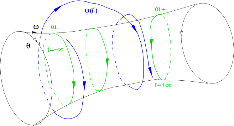
Figure 2: Convergence to stationary orbits.

Such an attraction was proved for the first time i) in [49]–[54] for the Klein–Gordon and Dirac equations coupled to $U(1)$-invariant nonlinear oscillator, ii) in [48], for discrete approximations of such coupled systems, i.e., for the corresponding difference schemes, and iii) in [57]–[59] for the wave, Klein–Gordon, and Dirac equations with concentrated nonlinearities. More precisely, we have proved global attraction to the solitary manifold of all stationary orbits, though global attraction to a particular stationary orbits, with fixed $\omega_{\pm}$, is still an open problem.

All these results were proved under the assumption that the equations are ‘strictly nonlinear’. For linear equations, the global attraction obviously fails if the discrete spectrum consists of at least two different eigenvalues.

The proofs of all these results rely on i) a nonlinear analog of the Kato theorem on the absence of embedded eigenvalues, ii) a new theory of multiplicators in the space of quasimeasures and iii) a novel application of the Titchmarsh convolution theorem.

4.3 Orthogonal group $G=SO(3)$

In this case (3.5) means the long-time asymptotics

$$\Psi(t)\sim e^{-i\hat{\Omega}_{\pm}t}\Psi_{\pm},\qquad t\to\pm\infty,$$ (4.9)

where $\hat{\Omega}_{\pm}$ are suitable representations of real skew-symmetric $3\times 3$ matrices $\Omega_{\pm}\in\mathfrak{so}(3)$. This means that global attraction to ‘stationary $SO(3)$-orbits’ occurs. Such asymptotics are proved in [60] for the Maxwell–Lorentz equations with rotating particle.
Generic equations. We must still specify the meaning of the term generic in our conjecture (3.5) In fact, this conjecture means that the asymptotics (3.5) hold for all solutions for an open dense set of $G$-invariant equations.
i) In particular, the asymptotics (4.1), (4.6), (4.8) and (4.9) hold under appropriate conditions, which define some ‘open dense subset’ of $G$-invariant equations with the four types of symmetry group $G$. This asymptotic expression may break down if these conditions fail — this corresponds to some ‘exceptional’ equations. For example, global attraction (4.8) breaks down for the linear Schrödinger equations with at least two different eigenvalues. Thus, linear equations are exceptional, not generic!
ii) The general situation is the following. Let a Lie group $G_{1}$ be a (proper) subgroup of some larger Lie group $G_{2}$. Then $G_{2}$-invariant equations form an ‘exceptional subset’ among all $G_{1}$-invariant equations, and the corresponding asymptotics (3.5) may be completely different. For example, the trivial group $\{e\}$ is a proper subgroup in $U(1)$ and in ${\mathbb{R}}^{n}$, and the asymptotic expressions (4.6) and (4.8) may differ significantly from (4.1).

5 Wave-particle duality

In his PhD of 1923, de Broglie suggested to identify the beam of particles with a harmonic wave:

$$\!\!\!\!\!\!\!\!\left.\!\!\!\!\!\!\!\!\begin{array}[]{c}\mbox{\it a beam of free particles with momentum $k$ and energy $E$ is described }\\ \mbox{\it with the wave function}\,\,\psi(x,t)=Ce^{i(kx-\omega t)},\,\,{where}\,\,k=p/\hbar,\,\,\omega=E/\hbar\end{array}\right|.$$ (5.1)

This identification was suggested by L. de Broglie for relativistic particles as a counterpart to the Einstein corpuscular treatment of light as a beam of photons.

The nonrelativistic version of this duality was the key source for the Schrödinger Quantum Mechanics. In this section, we discuss a possible treatment of this nonrelativistic wave-particle duality in the framework of semiclassical Maxwell–Schrödinger equations for the following phenomena: i) reduction of wave packets, ii) the diffraction of electrons, iii) acceleration of electrons in the electron gun.

5.1 Reduction of wave packets

We suggest an appearance of the wave-particle duality relying on a generalization of the conjecture (3.5) to the case of translation-invariant Maxwell–Schrödinger system (1.1) without external potentials, i.e., ${\bf A}_{\rm ext}(x,t)\equiv 0$, $A^{0}_{\rm ext}(x,t)\equiv 0.$ In this case, the Schrödinger equation of (1.1) becomes

$$i\hbar\dot{\psi}(x,t)=\frac{1}{2m}[-i\hbar\nabla\!-\!\displaystyle\frac{e}{c}{\bf A}(x,t)]^{2}\psi(x,t)\!+\!eA^{0}(x,t)\psi(x,t),\quad x\in{\mathbb{R}}^{3}.$$ (5.2)

Now the symmetry group of the system (1.1) is $G={\mathbb{R}}^{3}\times U(1)$, and our general conjecture (3.5) should be strengthened similarly to (4.7) as the long-time asymptotics of each finite energy solution

$$\!\!\!{\bf A}(x,t)\!\sim\!\displaystyle\!\sum\limits_{k}{\bf A}_{\pm}^{k}(x\!-\!v^{k}_{\pm}t)+{\bf A}_{\pm}(x,t),\,\,\psi(x,t)\!\sim\!\displaystyle\!\sum\limits_{k}\psi_{\pm}^{k}(x\!-\!v^{k}_{\pm}t)e^{i\Phi_{\pm}^{k}(x,t)}\!+\!\psi_{\pm}(x,t)$$ (5.3)

as $t\to\pm\infty$, where ${\bf A}_{\pm}(x,t)$ and $\psi_{\pm}(x,t)$ stand for the corresponding dispersion waves. These asymptotics are considered in global energy norms, and suggest to treat the solitons

$$({\bf A}_{\pm}^{k}(x\!-\!v^{k}_{\pm}t),\psi_{\pm}^{k}(x\!-\!v^{k}_{\pm}t)e^{i\Phi_{\pm}^{k}(x,t)})$$ (5.4)

as electrons. These asymptotics provisionally correspond to the reduction (or collapse) of wave packets.

5.2 Diffraction of electrons

The most striking and direct manifestation of particle-wave duality is given by diffraction of electrons observed by C. Davisson and L. Germer in their experiments of 1924–1927s. In these first experiments, the electron beam was scattered by a crystal of nickel, and the reflected beam was fixed on a film. The resulting images are similar to X-ray scattering patterns (‘lauegrams’), first obtained in 1912 by the method of Laue. These experiments were the main motivation for Born’s introduction of the probabilistic interpretation of the wave function.

Later on, such experiments were also carried out with transmitted electron beams scattered by thin gold and platinum crystalline films (G. P. Thomson, the 1937 Nobel Prize). Only recently R. Bach with collaborators first carried out the two-slit diffraction of electrons [21] as is illustrated by Fig. 3.

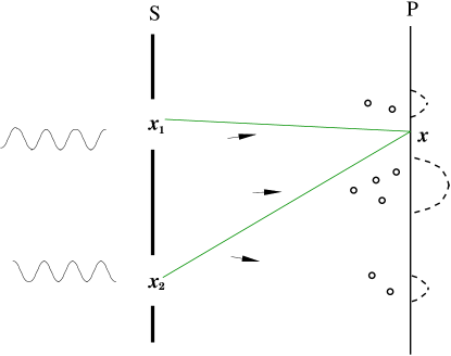
Figure 3: Diffraction by double-slit.

The traditional description of these experiments relies on the following scheme:
I. The incident beam of electrons emitted by an electron gun is described by the plane wave

$$\psi^{in}(x,t)=Ce^{i(kx-\omega t)}$$ (5.5)

satisfying the free Schrödinger equation, with wave number $k$ and frequency $\omega$ given by the de Broglie relations (5.1).
II. The diffraction of a plane wave in reflection by a crystal or in scattering by an aperture in the scattering screen.
III. The observation of the diffraction amplitude on the screen of registration.

We show in Section 5.3 below that the formation of the incident plane wave (5.5) in the electron gun can be explained by the quasiclassical asymptotics for the linear Schrödinger equation.

Further, the diffraction in step II is traditionally described by the linear Schrödinger equation, see [23]–[27]. According to the limiting amplitude principle, the diffracted wave admits the asymptotics

$$\psi_{d}(x,t)\sim a_{\infty}(x)e^{-i\omega t},\qquad t\to\infty,$$ (5.6)

where $\omega$ is the frequency of the incident wave (5.5). We calculated the diffraction amplitudes $a_{\infty}(x)$ in the case of diffraction by the screen using the Kirchhoff approximation (formulas (2.7.15) and (2.7.16) of [22]). In particular, for the two-slit diffraction, the corresponding amplitude [22, (2.7.20)] is in a fine quantitative agreement with the results of recent diffraction experiments [21]. Indeed, the maxima of $|a_{\infty}(x)|$ on the screen agree very well with that of the diffraction pattern in experiments [21].

Thus, the arguments above rely on the linear Schrödinger theory. On the other hand, the formation of the diffraction pattern in the step III is a genuinely nonlinear effect of the reduction of wave packets which can be interpreted as the soliton asymptotics (5.3) for solutions of the coupled nonlinear Maxwell–Schrödinger equations.

5.3 Quasiclassical asymptotics for electron gun

Here we justify the incident wave function (5.5) for electrons emitted by an electron gun. The hot cathode emits electrons of small energy and after which the electrons are accelerated in an electrostatic field ${\bf E}(x)=-\nabla\Phi(x)$ in the region $\Omega_{1}$ between the cathode and anode. The electrons cross the region $\Omega_{1}$ and pass through an aperture in the anode into the region $\Omega_{2}$ behind the anode, where the field ${\bf E}(x)$ vanishes. In this region, the electrons interfere, forming a diffraction pattern.

We will show that the diffraction amplitude coincides with the one corresponding to the free Schrödinger equation in the region $\Omega_{2}$ with the incident wave (5.5) at the points of the aperture, where the corresponding wave vector $k$ and frequency $\omega$ are given by de Broglie’s formulas (5.1). In this case, $E$ and $p$ denote the kinetic energy and momentum of the classical electron at the points of the aperture.

Namely, the electron wave function in the region $\Omega_{1}\cup\Omega_{2}$ is a solution to the corresponding Schrödinger equation

$$i\hbar\dot{\psi}(x,t)=-\frac{\hbar^{2}}{2{\rm m}}\Delta\psi(x,t)+e\Phi(x)\psi(x,t),\quad x\in\Omega_{1}\cup\Omega_{2},$$ (5.7)

where $\Phi(x)$ is the electrostatic potential vanishing on the cathode. This potential is constant in $\Omega_{2}$, where the electrostatic field vanishes, so the equation (5.7) behind the anode reads

$$i\hbar\dot{\psi}(x,t)=-\frac{\hbar^{2}}{2{\rm m}}\Delta\psi(x,t)+e\Phi_{*}\psi(x,t),\qquad x\in\Omega_{2},$$ (5.8)

where $\Phi_{*}$ is the value of the potential $\Phi(x)$ at the points of the aperture. Further, we suppose that the solution admits the quasiclassical asymptotics

$$\psi(x,t)\sim a(x,t)e^{i\frac{S(x,t)}{\hbar}},\qquad\hbar\to 0,$$ (5.9)

where $a(x,t)$ and $S(x,t)$ are slowly varying fuctions. Substituting into (5.7), we obtain in the limit $\hbar\to 0$ the corresponding Hamilton–Jacobi equation for the phase function

$$-\partial_{t}S(x,t)=\frac{1}{2{\rm m}}[\nabla S(x,t)]^{2}+e\Phi(x),\quad x\in\Omega_{1}.$$ (5.10)

The solution is given by the action integral over classical trajectories which satisfy the Hamiltonian equations

$$\dot{x}(t)=p(t)/{\rm m},\qquad\dot{p}(t)=-e\nabla\Phi(x(t)),$$ (5.11)

corresponding to the Hamiltonian function

$$H(x,p)=\frac{1}{2{\rm m}}p^{2}+e\Phi(x).$$ (5.12)

In particular, let us consider the trajectories of emitted classical electrons starting at time $t_{0}$ from all points $x(t_{0})$ of the cathode with momentum $p(t_{0})$ and passing trough the aperture at the time $t_{*}=t_{0}+T$. The initial data at time $t_{0}$ are related by $p(t_{0})=\nabla S(x(t_{0}))$ for all possible initial points $x(t_{0})$. Hence we have for all trajectories,

$$\nabla S(x(t),t)=p(t)$$ (5.13)

which follows from the Hamilton–Jacobi equation (5.10) (see [8, 9]). The initial kinetic energy of the emitted electrons is small, so we can assume that

$$H(x(t_{0}),p(t_{0}))=0.$$ (5.14)

Let us denote $x_{*}:=x(t_{*})$ and $p_{*}:=p(t_{*})$. By the energy conservation, we also have $H(x_{*},p_{*})=0$, and hence,

$$\frac{1}{2{\rm m}}p_{*}^{2}=-e\Phi_{*},\qquad\partial_{t}S(x_{*},t_{*})=0,$$ (5.15)

where the last identity follows from the Hamilton–Jacobi equation (5.10) with $x=x_{*}$ and $t=t_{*}$. Now the Taylor expansion gives

$$S(x,t)\approx S(x_{*},t_{*})+p_{*}(x-x_{*}),\qquad|x-x_{*}|+|t-t_{*}|\ll 1,$$ (5.16)

since $\partial_{t}S(x_{*},t_{*})=0$ by (5.15) and

$$\nabla S(x_{*},t_{*})=p_{*}$$ (5.17)

by (5.13). Therefore, at the points of the aperture the wave function reads

$$\psi(x,t)=a(x_{*},t_{*})e^{iS(x_{*},t_{*})/\hbar}e^{ip_{*}(x-x_{*})/\hbar}\approx Ce^{ip_{*}x/\hbar},$$ (5.18)

since $a(x_{*},t_{*})$ and $S(x_{*},t_{*})$ are slowly varying functions.

Finally, the electrostatic potential $\Phi_{*}$ in the Schrödinger equation (5.8) behind the screen can be eliminated by the gauge transform

$$\psi(x,t)\mapsto\psi_{*}(x,t):=\psi(x,t)e^{ie\Phi_{*}t/\hbar}.$$ (5.19)

Indeed, the transformed function $\psi_{*}(x,t)$ behind the screen satisfies the free Schrödinger equation

$$i\hbar\dot{\psi}_{*}(x,t)=-\frac{\hbar^{2}}{2{\rm m}}\Delta\psi_{*}(x,t),\qquad x\in\Omega_{2}.$$ (5.20)

The key observation is that we have the following asymptotics at the points of the small aperture

$$\psi_{*}(x,t):=\psi(x,t)e^{ie\Phi_{*}t/\hbar}\approx Ce^{ip_{*}x/\hbar}e^{ie\Phi_{*}t/\hbar}=Ce^{i(p_{*}x-E_{*}t)/\hbar}$$ (5.21)

which follows from (5.19) and (5.18); here

$$E_{*}=-e\Phi_{*}$$ (5.22)

is the energy of the classical electron at the aperture, and $p_{*}$ is its momentum. This justifies the asymptotics of type (5.5) for $\psi(x,t)$ at the points of the aperture with

$$k=p_{*}/\hbar,\qquad\omega=E_{*}/\hbar$$ (5.23)

which are exactly the de Broglie relations (5.1). Finally, the diffraction pattern corresponding to the charge densities $e|\psi(x,t)|^{2}$ and $e|\psi_{*}(x,t)|^{2}$ behind the aperture coincide by (5.19) and the Born rule (6.1).

Remark 5.1.

Note that the relations (5.22), (5.23) together with the first equation of (5.15) imply that

$$\hbar\omega=\frac{\hbar^{2}k^{2}}{2{\rm m}},$$ (5.24)

that is the incident wave (5.5) satisfies the free Schrödinger equation.

6 Probabilistic interpretation

In 1927, M. Born suggested the Born rule which is probabilistic interpretation of the wave function:

$$\left.\begin{array}[]{c}\mbox{\it The probability of detecting an electron at a point $x$ at time $t$}\\ \mbox{\it is proportional to $|\psi(x,t)|^{2}$.}\end{array}\right|$$ (6.1)

6.1 Diffraction current

M. Born proposed the probabilistic interpretation to describe the diffraction experiments of C. Davisson and L. Germer of 1924–1927s. Let us demonstrate that the rule (6.1) can be explained in the framework of these experiments by calculating the current (1.2) at the points of the screen of registration.

Indeed, the diffraction pattern is registered either by atoms of photo emulsion or by registration counters located on the screen. In all cases the rate of registration is proportional to the current density by definition. Thus, to explain the Born rule (6.1) in this situation, we must to show that the current density (1.2) on the screen of registration is proportional to $|\psi(x,t)|^{2}$:

$${\bf j}(x,t)\sim|\psi(x,t)|^{2}(0,0,1)$$ (6.2)

if the screen lies in the plane $x_{3}={\rm const}$. The current density (1.2) is approximately given by

$${\bf j}(x,t)\approx\frac{e}{{\rm m}}\psi(x,t)\cdot[-i\hbar\nabla\psi(x,t)].$$ (6.3)

Indeed, in formula (1.2), we have ${\bf A}^{\rm ext}(x,t)=0$ since there is no external fields between the scatterer screen and the screen of observation. The term with ${\bf A}(x,t)$ in (1.2) is neglected, since its contribution contains an additional small factor $\frac{e}{c}$.

For large times, the wave function is given by the limiting amplitude principle

$$\psi(x,t)\sim a_{\infty}(x)e^{-i\omega t},\qquad t\to\infty.$$ (6.4)

The limiting amplitude $a_{\infty}(x)$ near the diffraction screen is given by formula

$$a_{\infty}(x)\sim-\frac{ika_{in}(1+\cos\overline{\chi})e^{ik|x|}}{(4\pi)^{2}|x|}\int_{Q}e^{-ik(\xi_{1}y_{1}+\xi_{2}y_{2})}dy,\qquad|x|\to\infty$$ (6.5)

similar to formula (28) of [2, Section 8.3.3] which describes the Fraunhofer diffraction. Here $(\xi_{1},\xi_{2},\xi_{3}):=x/|x|$ and $\cos\overline{\chi}=\xi_{3}>0$; $Q$ is the aperture in the scattering plane $x_{3}=0$ and the diffraction screen lies in the plane $x_{3}={\rm const}\gg 1$. This formula implies that for bounded $|(x_{1},x_{2})|\leq C$ the limiting amplitude admits the following asymptotic representation,

$$a_{\infty}(x)\sim\frac{b(\xi_{1},\xi_{2})}{|x|}e^{ikx_{3}},\qquad x_{3}\to\infty.$$ (6.6)

Here the amplitude $b(\xi_{1},\xi_{2})$ is a slowly varying function of transversal variables $(x_{1},x_{2})$ for large $x_{3}$, so asymptotically

$$\nabla a_{\infty}(x)\sim ika_{\infty}(x)(0,0,1)\quad\mbox{\rm for }|(x_{1},x_{2})|\leq C\quad{\rm and}\quad x_{3}\to\infty.$$ (6.7)

Hence, (6.3) gives

$${\bf j}(x,t)\approx\frac{e\hbar|k|}{{\rm m}}|a_{\infty}(x)|^{2}(0,0,1),\qquad t\to\infty$$ (6.8)

since the screen of registration is sufficiently far from the screen of scattering. Finally, (6.4) implies that for large times we have $|a_{\infty}(x)|^{2}\approx|\psi(x,t)|^{2}$, so (6.8) implies (6.2), which explains the Born rule (6.1).

Remark 6.1.

Our arguments above justify the Born rule (6.1) in the framework of the diffraction experiments with a plane screen in the configuration of Fig. 3. For a curved screen, the same arguments suggest that the rate of registration is proportional to the current and to $\cos\theta$, where $\alpha$ is the angle of incidence (the angle between the direction of the electron beam and the normal to the screen).

6.2 Discrete registration of electrons

In 1948, the probabilistic interpretation was given new content and confirmation by the experiments of L. Biberman, N. Sushkin and V. Fabrikant [17] with an electron beam of very low intensity. Later, similar experiments were carried out by R. Chambers, A. Tonomura, S. Frabboni, R. Bach and others [18, 19, 20, 21]. In these experiments, the diffraction pattern is created as an average in time of random discrete registration of individual electrons.

We suggest below two possible treatments of the probabilistic interpretation in these experiments. These treatments rely respectively
i) on a random interaction with the counters, and
ii) on the soliton conjecture (5.3) in the framework of the coupled translation-invariant Maxwell–Schrödinger equations (1.1).

However, the corresponding rigorous justification is still an open problem.
I. Interaction with counters. One possible explanation of the discrete registration is a random triggering of a) registration counters located at the screen points, or b) atoms of the photo emulsion. In both cases, the probability of triggering must be proportional to the electric current near the screen of observation.
II. Reduction of wave packets. In the space between the scatterer screen and the screen of observation, the external fields vanish. Hence, in this space, the Maxwell–Schödinger system is translation-invariant, which is the case of our conjecture (5.3) on the decay to solitons–electrons (5.4), see Fig. 3. Such a decay should be regarded as a random process, since it is subject to microscopic fluctuations.

6.3 Superposition principle as the linear approximation

The treatment II of the discrete registration of electrons in the previous section is not self-consistent. Indeed, the justification of the formula (6.8) relies on the linear Schrödinger equation, while the reference to the soliton asymptotics (5.3) involves the nonlinear Maxwell–Schrödinger equations.

We suggest the following argument reconciling this formal contradiction: formula (6.8) holds in the linear approximation, while the soliton asymptotics (5.3) holds in the next approximation of the nonlinear Maxwell–Schrödinger equations.

Remark 6.2.

The formula (6.8) for the linear Schrödinger equation relies on the superposition principle which is the traditional argument claiming that quantum mechanics is absolutely linear! On the other hand, the discrete registration of electrons cannot be described by the linear Schrödinger equation.

Acknowledgements. The author thanks Sergey Kuksin, Alexander Shnirelman and Herbert Spohn for long-term discussions.

References

Faculty of Mathematics, University of Vienna, Oskar-Morgenstern-Platz 1, 1090 Wien, Austria. e-mail: alexander.komech@univie.ac.at

References

- [1] N. Bohr, Discussion with Einstein on epistemological problems in atomic physics, pp 201–241 in: Schilpp, P.A., Ed., Albert Einstein: Philosopher-Scientist, Vol 7, Library of Living Philosophers, Evanston Illinois, 1949. Quantum Mechanics
- [2] M. Born, E. Wolf, Principles of Optics, Cambridge University Press, Cambridge, 1966.
- [3] A. Einstein, P. Ehrenfest, Quantentheoretische Bemerkungen zum Experiment von Stern und Gerlach, Zeitschrift für Physik 11 (1922), 31–34.
- [4] A. Komech, Quantum Mechanics: Genesis and Achievements, Springer, Dordrecht, 2013.
- [5] J.J. Sakurai, Advanced Quantum Mechanics, Addison-Wesley, Reading, Massachusets, 1967.
- [6] H. Spohn, Dynamics of Charged Particles and their Radiation Field, Cambridge University Press, Cambridge, 2004.
- [7] E. Schrödinger, Quantisierung als Eigenwertproblem, Ann. d. Phys. I, II 79 (1926) 361, 489; III 80 (1926) 437; IV 81 (1926) 109. (English translation in E. Schrödinger, Collected Papers on Wave Mechanics, Blackie & Sohn, London, 1928.) Differential equations
- [8] V. I. Arnold, Mathematical Methods of Classical Mechanics, Springer, New York, 1989.
- [9] H. Goldstein, C.P. Poole, J. Safko, Pearson, New York, 2001.
- [10] A.I. Komech, E.A. Kopylova, Dispersion Decay and Scattering Theory, Wiley, Hoboken, New Jersey, 2012. Maxwell–Schrödinger equations
- [11] I. Bejenaru, D. Tataru, Global well-posedness in the energy space for the Maxwell–Schrödinger system, Commun. Math. Phys. 288 (2009), 145–198.
- [12] R. D. Jackson, Classical Electrodynamics, Wiley, New York, 1999.
- [13] M. O. Scully, M. S. Zubairy, Quantum Optics, Cambridge university press, Cambridge, 1997.
- [14] Y. Guo, K. Nakamitsu, W. Strauss, Global finite-energy solutions of the Maxwell–Schrödinger system, Comm. Math. Phys. 170 (1995), no. 1, 181–196.
- [15] G. M. Coclite, V. Georgiev, Solitary waves for Maxwell–Schrödinger equations, Electronic Journal of Differential Equations 94 (2004), 1–31. arXiv:math/0303142 [math.AP]
- [16] M. Nakamura, T. Wada, Global existence and uniqueness of solutions to the Maxwell–Schrödinger equations, Comm. Math. Phys. 276 (2007), 315–339. Diffraction of electrons
- [17] L. Biberman, N. Sushkin, V. Fabrikant, Diffraction of successively travelling electrons, Doklady AN SSSR 66 (1949), no.2, 185–186, 1949.
- [18] R. G. Chambers, Shift of an electron interference pattern by enclosed magnetic flux, Physical Review Letters 5 (1960), 3–5.
- [19] A. Tonomura, J. Endo, T. Matsuda, T. Kawasaki, H. Ezawa, Demonstration of single-electron buildup of an interference pattern, Amer. J. Phys. 57 (1989), no. 2, 117–120.
- [20] S. Frabboni, G. C. Gazzadi, G. Pozzi, Young’s double-slit interference experiment with electrons, Amer. J. Phys. 75 (2007), Issue 11, 1053–1055.
- [21] R. Bach, D. Pope, S.-H. Liou, H. Batelaan, Controlled double-slit electron diffraction, New J. Phys. 15 (2013), 033018. http://iopscience.iop.org/1367-2630/15/3/033018/media/njp458349suppdata.pdf
- [22] A. Komech, Lectures on Quantum Mechanics for Mathematicians. arXiv math-ph 1907.05786 Shift of Aharonov-Bohm
- [23] W. Ehrenberg, R.E. Siday, The Refractive Index in Electron Optics and the Principles of Dynamics, Proc. Phys. Soc., Section B, 62 (1949), 8–21.
- [24] Y. Aharonov, D. Bohm, Significance of electromagnetic potentials in the quantum theory, Phys. Rev. 115 (1959), no. 3, 485–491.
- [25] S. Olariu, I. I. Popesku, The quantum effects of electromagnetic fluxes, Rev. Mod. Phys. 57 (1985), 339–436.
- [26] M. Peshkin, A. Tonomura, The Aharonov–Bohm Effect, Lecture Notes in Physics, Vol. 340, Springer, Berlin, 1989.
- [27] B. Helffer, Effet d’Aharonov Bohm sur un état borné de l’Equation de Schrödinger, Comm. Math. Phys. 119 (1988), 315–329. Omega-Hyperon
- [28] M. Gell-Mann, Symmetries of baryons and mesons, Phys. Rev. (2) 125 (1962), 1067–1084.
- [29] Y. Ne’eman, Unified interactions in the unitary gauge theory, Nuclear Phys. 30 (1962), 347–349.
- [30] F. Halzen and A. Martin, Quarks and leptons: an introductory course in modern particle physics, John Wiley & Sons, New York, 1984.
- [31] V. E. Barnes & al., Observation of a hyperon with strangeness minus three, Phys. Rev. Lett. 12 (1964), 204–206. Global attractors of dissipative PDEs
- [32] L. Landau, On the problem of turbulence, C. R. (Doklady) Acad. Sci. URSS (N.S.) 44 (1944), 311–314.
- [33] A. V. Babin and M. I. Vishik, Attractors of Evolution Equations, vol. 25 of Studies in Mathematics and its Applications, North-Holland Publishing Co., Amsterdam, 1992.
- [34] V.V. Chepyzhov and M.I. Vishik, Attractors for Equations of Mathematical Physics, vol. 49 of American Mathematical Society Colloquium Publications, American Mathematical Society, Providence, RI, 2002.
- [35] R. Temam, Infinite-Dimensional Dynamical Systems in Mechanics and Physics, Springer, New York, 1997. Global attraction to stationary states
- [36] A.I. Komech, On the stabilization of interaction of a string with a nonlinear oscillator, Moscow Univ. Math. Bull. 46 (1991), no. 6, 34–39.
- [37] A.I. Komech, On stabilization of string-nonlinear oscillator interaction, J. Math. Anal. Appl., 196 (1995), 384–409.
- [38] A. Komech, On transitions to stationary states in one-dimensional nonlinear wave equations, Arch. Ration. Mech. Anal. 149 (1999), 213–228.
- [39] A. Komech, H. Spohn, M. Kunze, Long-time asymptotics for a classical particle interacting with a scalar wave field, Comm. Partial Differential Equations 22 (1997), 307–335.
- [40] A. Komech, H. Spohn, Long-time asymptotics for the coupled Maxwell–Lorentz equations, Comm. Partial Differential Equations 25 (2000), 559–584.
- [41] I.M. Sigal, Nonlinear wave and Schrödinger equations. I. Instability of periodic and quasiperiodic solutions, Comm. Math. Phys. 153 (1993), 297–320. Global attraction to solitons
- [42] W. Eckhaus, A. van Harten, The Inverse Scattering Transformation and the Theory of Solitons, vol. 50 of North-Holland Mathematics Studies, North-Holland Publishing Co., Amsterdam–New York, 1981.
- [43] A. Komech, H. Spohn, Soliton-like asymptotics for a classical particle interacting with a scalar wave field, Nonlinear Anal. 33 (1998), 13–24.
- [44] V. Imaykin, A. Komech, N. Mauser, Soliton-type asymptotics for the coupled Maxwell-Lorentz equations, Ann. Henri Poincaré P (2004), 1117–1135.
- [45] V. Imaykin, A. Komech, H. Spohn, Scattering theory for a particle coupled to a scalar field, Discrete Contin. Dyn. Syst. 10 (2004), 387–396.
- [46] A.I. Komech, N.J. Mauser, A.P. Vinnichenko, Attraction to solitons in relativistic nonlinear wave equations, Russ. J. Math. Phys. 11 (2004), 289–307.
- [47] G.L. Lamb Jr., Elements of soliton theory, John Wiley & Sons, Inc., New York, 1980. Global attraction to stationary orbits
- [48] A. Comech, Weak attractor of the Klein-Gordon field in discrete space-time interacting with a nonlinear oscillator, Discrete Contin. Dyn. Syst. 33 (2013), 2711–2755.
- [49] A.I. Komech, On attractor of a singular nonlinear -invariant Klein–Gordon equation, in Progress in analysis, Vol. I, II (Berlin, 2001), World Sci. Publ., River Edge, NJ, 2003, 599–611.
- [50] A.I. Komech, A.A. Komech, On the global attraction to solitary waves for the Klein–Gordon equation coupled to a nonlinear oscillator, C. R. Math. Acad. Sci. Paris 343 (2006), 111–114.
- [51] A. Komech, A. Komech, Global attractor for a nonlinear oscillator coupled to the Klein–Gordon field, Arch. Ration. Mech. Anal. 185 (2007), 105–142.
- [52] A. Komech, A. Komech, On global attraction to solitary waves for the Klein–Gordon field coupled to several nonlinear oscillators, J. Math. Pures Appl. (9) 93 (2010), 91–111.
- [53] A. Komech, A. Komech, Global attraction to solitary waves for Klein-Gordon equation with mean field interaction, Ann. Inst. H. Poincaré Anal. Non Linéaire 26 (2009), 855–868.
- [54] A. Komech, A. Komech, Global attraction to solitary waves for a nonlinear Dirac equation with mean field interaction, SIAM J. Math. Anal. 42 (2010), 2944–2964.
- [55] A.I. Komech, Attractors of nonlinear Hamilton PDEs, Discrete and Continuous Dynamical Systems A 36 (2016), no. 11, 6201–6256. arXiv:1409.2009
- [56] A.I. Komech, E. A. Kopylova, Attractors of Hamiltonian nonlinear partial differential equations, Russ. Math. Surv. 75 (2020), no. 1, 1–87.
- [57] E. Kopylova, Global attraction to solitary waves for Klein–Gordon equation with concentrated nonlinearity, nonlinearity 30 (2017), no. 11, 4191–4207.
- [58] E. Kopylova, A.I. Komech, On global attractor of 3D Klein–Gordon equation with several concentrated nonlinearities Dynamics of PDE, 16 (2019), no. 2, 105–124.
- [59] E. Kopylova, A. Komech, Global attractor for 1D Dirac field coupled to nonlinear oscillator, Comm. Math. Phys. 375 (2020), no. 1, 573–603. Open access. http://link.springer.com/article/10.1007/s00220-019-03456-x
- [60] V. Imaykin, A. Komech, H. Spohn, Rotating charge coupled to the Maxwell field: scattering theory and adiabatic limit, Monatsh. Math. 142 (2004), 143–156.