Quench Dynamics in 1D Optomechanical Arrays

Abstract

Non-equilibrium dynamics induced by rapid changes of external parameters is relevant for a wide range of scenarios across many domains of physics. For waves in spatially periodic systems, quenches will alter the bandstructure and generate new excitations. In the case of topological bandstructures, defect modes at boundaries can be generated or destroyed when quenching through a topological phase transition. Here, we demonstrate that optomechanical arrays are a promising platform for studying such dynamics, as their bandstructure can be tuned temporally by a control laser. We study the creation of nonequilibrium optical and mechanical excitations in 1D arrays, including a bosonic version of the Su-Schrieffer-Heeger model. These ideas can be transferred to other systems such as driven nonlinear cavity arrays.

I Introduction

Cavity optomechanics Aspelmeyer et al. (2014) exploits the radiation pressure interaction to couple optical and mechanical degrees of freedom. A centerpiece of the physics encountered in this setting is the parametric nature of the optomechanical interaction: the radiation force is quadratic in the light amplitude. Upon driving such a system by a control laser field, this results in an effective laser-enhanced linear coupling between optics and mechanics. Importantly, that coupling is tuneable by the control laser amplitude. This tuneability sets optomechanical systems apart from resonantly coupled light-matter systems, and it offers time-dependent optical control, which is beneficial in a large range of scenarios, including (as we will show) the study of quench physics.

Leaving behind the standard system of one optical mode coupled to one mechanical mode, we arrive at optomechanical arrays (see e.g. Bhattacharya and Meystre (2008); Chang et al. (2011); Heinrich et al. (2011); Xuereb et al. (2012a); Ludwig and Marquardt (2013); Chen and Clerk (2014); Peano et al. (2015); Zapletal et al. (2018); Piergentili et al. (2018); McDonald et al. (2018); Yanay and Clerk (2018); Bemani et al. (2019) ). These are comprised of a set of coupled vibrational and optical modes. They can be realized using a variety of building blocks, like photonic crystal defect cavities or microdisk resonators (in the optical domain), or microwave-optomechanical circuits. Although experimentally still in their infancy Zhang et al. (2012, 2015); Fang et al. (2017); Piergentili et al. (2018); Naserbakht et al. (2019), a variety of promising future directions and applications have been identified theoretically, covering phenomena like bandstructure engineering Chang et al. (2011); Schmidt et al. (2015a), topological transport Peano et al. (2015); Zapletal et al. (2018); McDonald et al. (2018), coupling enhancement Xuereb et al. (2012b, 2013); Li et al. (2016), Anderson localization Roque et al. (2017), synchronization Heinrich et al. (2011); Holmes et al. (2012), and quantum information processingSchmidt et al. (2012).

The propagation of photons and phonons in an optomechanical array is described by a bandstructure of hybrid photon-phonon excitations. This bandstructure depends on the geometry and the underlying intrinsic coupling of neighboring optical and mechanical modes. However, on top of that, it is also determined by the external control laser illuminating the array.

In the present work, we demonstrate how time-dependent optical control of an optomechanical array can induce nonequilibrium dynamics triggered by non-adiabatic changes in the bandstructure. There are several actively tunable degrees of freedom in optomechanical arrays that can change the bandstructure, e.g. power and phase of the external laser, which means that they offer great promise for studying non-adiabatic dynamics Schmidt et al. (2012); Brunelli et al. (2015); Schmidt et al. (2015b); Walter and Marquardt (2016).

In general, nonequilibrium physics produced upon changes of a Hamiltonian’s parameters is encountered in many different physical scenarios, ranging from the evolution of fields in the expanding early universe to quenches through phase transitions upon rapid cooling of a substance Polkovnikov et al. (2011); Eisert et al. (2015); Mitra (2017). When the parameters of a bandstructure are changed, existing equilibrium excitations will be redistributed. If the quench takes the bandstructure through a topological phase transition, in a finite system topological states can be created or destroyed at the boundaries. We will show that this kind of physics can be explored in optomechanical arrays. Among our examples of 1D arrays, we will present a design for an optomechanical Su-Schrieffer-Heeger model Su et al. (1979), where 0D edge states exist Atala et al. (2013); Meier et al. (2016). This model is considered to be the simplest example of a bandstructure with topological properties Asbóth et al. (2016).

Quenches through topological phase transitions have recently attracted a lot of attention Sharma et al. (2016); Sun et al. (2018); Schüler et al. (2018); Gong and Ueda (2018). It is interesting to understand how different properties of many-body systems, such as integrability Iyer et al. (2013); Essler et al. (2014); Kormos et al. (2017) or topological order Tsomokos et al. (2009); Budich and Heyl (2016); Wilson et al. (2016); Sharma et al. (2016) interplay with non-equilibrium dynamics of these systems andhow topological properties such as the Chern number or Berry phase would evolve through a quench Yang et al. (2018); Chen et al. (2019); Liou and Yang (2018). For instance, Ciao et al. investigated some of these questions in the Haldane model Caio et al. (2015). Similar investigations has been done for the SSH model in cold atoms Meier et al. (2016).

Although optical lattice experiments (like Meier et al. (2016); Atala et al. (2013)) are naturally suited for studying quench physics and topological phases, we believe our work shows it is worthwhile to extend such studies to optomechanical systems. Not only do they offer different forms of access (e.g. via the light emitted from the array), but they also involve physics that cannot easily be investigated in cold atom systems. This includes the effects of a thermal environment on the quench dynamics, or the possibility to add superconducting qubits (in microwave optomechanics realizations of optomechanical arrays Teufel et al. (2008); Regal et al. (2008); Teufel et al. (2011a); Pirkkalainen et al. (2013)).

The structure of this paper is as follows. We start by describing a 1D optomechanical array and investigate the quench dynamics in this array. This not only helps us understand the dynamical properties of this particular system, but can also be used for other scenarios in which optomechanical arrays are driven out of equilibrium. Afterwards, we turn to the SSH model. After explaining the basics of the model, we provide a design for an optomechanical simulator that mimics the Hamiltonian of the SSH model and can also be tuned dynamically. Finally, we describe an example of a simple quench experiment that can be carried out using this simulator and describe the expected outcomes of the experiment.

II Quenches in optomechanical arrays

II.1 Model

II.1.1 Hamiltonian

An optomecanical array is an array of optomechanical cells that are connected through optical and vibrational couplings. Figure (1) gives a schematic picture of a simple optomechanical array. Blue circles represent the optical cavities with the frequency detuning $\Delta$ from the external laser and decay rate $\kappa$. Yellow circles represent the mechanical resonators with the frequency $\Omega$ and dissipation rate $\Gamma$. The (laser-enhanced) optomechanical coupling between the mechanics and optics is given by $g$. Furthermore, optical cavities and mechanical resonators on different sites are coupled to each other and the strength of the coupling is given by $K$ and $J$ for the mechanical and optical modes between different sites. The full Hamiltonian of this system can be written as

$$H_{OMA} =\sum_{i}\left(-\hbar\Delta\hat{a}_{i}^{\dagger}\hat{a}_{i}+\hbar\Omega\hat{b}_{i}^{\dagger}\hat{b}_{i}\right)$$

$$-\hbar\sum_{i}g\left(\hat{a}_{i}^{\dagger}\hat{b}_{i}+\hat{a}_{i}\hat{b}_{i}^{\dagger}\right)$$

$$+\hbar J\sum_{i}\left(\hat{a}_{i}^{\dagger}\hat{a}_{i+1}+\hat{a}_{i}\hat{a}_{i+1}^{\dagger}\right)$$

$$+\hbar K\sum_{i}\left(\hat{b}_{i}^{\dagger}\hat{b}_{i+1}+\hat{b}_{i}\hat{b}_{i+1}^{\dagger}\right).$$ (1)

Here $\hat{a}_{i}$ and $\hat{b}_{i}$ are the annihilation operators corresponding to the optical and mechanical modes on site $i$ respectively. Note that this is the linearised Hamiltonian and the Hamiltonian is quadratic. The array can take any geometrical form. The Hamiltonian in Eq. (II.1.1) describes the lattice given in figure (1).

Figure 1: Schematic picture of a 1D optomechanical array. The blue and yellow circles represent the optical and mechanical modes respectively. Note that although schematically we separated them spatially, they may occupy the same physical space. Blue/yellow links, represent the optical/mechanical coupling between different sites of the lattice and red links show the optomechanical coupling on each site.

This system can be experimentally realized, for instance using optomechanical crystals Safavi-Naeini et al. (2014).

For most of this paper, we consider an ideal system with $\kappa\ll g$, which represents the strong coupling regime. We also assume that we are working in the red-detuned regime where the amplification terms in the Hamiltonian average out. Towards the end of this section, we will revisit these assumptions and consider the effects of large cavity dissipation and address how detuning would affect our results.

For simplicity, we Fourier-transform the Hamiltonian and rewrite it in terms of pseudo-momentum creation and annihilation operators which gives

$$H_{OMA} =\hbar\sum_{k}\left(-\Delta\left(k\right)\hat{a}_{k}^{\dagger}\hat{a}_{k}\right)$$ (2)

$$+\hbar\sum_{k} \left(\Omega\left(k\right)\hat{b}_{k}^{\dagger}\hat{b}_{k}+g\left(\hat{a}_{k}^{\dagger}\hat{b}_{k}+\hat{a}_{k}\hat{b}_{k}^{\dagger}\right)\right).$$ (3)

Here $\Delta\left(k\right)=\Delta-2J\cos\left(k\right)$ and $\Omega\left(k\right)=\Omega+2K\cos\left(k\right)$.

The Hamiltonian in Eq. (3) is a good approximation for large enough lattices or periodic BC or the bulk of the lattice, where there is translational invariance and $k$ is a good quantum number.

The Hamiltonian in Eq. (3) is similar to a single optomechanical cell and therefore, our results can be extended to optomechanical systems as well.

To study the normal modes of this system, we rewrite the Hamiltonian in terms of the Bloch Hamiltonian, $h_{k}$, i.e.

$$H_{OMA}=\sum_{k}\hbar\left(\begin{array}[]{cc}\hat{a}_{k}^{\dagger}&\hat{b}_{k}^{\dagger}\end{array}\right)h_{k}\left(\begin{array}[]{c}\hat{a}_{k}\\ \hat{b}_{k}\end{array}\right),$$ (4)

with

$$h_{k}=\left(\begin{array}[]{cc}-\Delta\left(k\right)&g\\ g&\Omega\left(k\right)\end{array}\right).$$ (5)

This can be rewritten as

$$h_{k}=\frac{\Omega\left(k\right)-\Delta\left(k\right)}{2}\mathcal{I}-\frac{\Omega\left(k\right)+\Delta\left(k\right)}{2}\sigma_{z}+g\sigma_{x},$$ (6)

with $\mathcal{I}$ the identity matrix and $\sigma_{x}$ and $\sigma_{z}$ the Pauli matrices for $X$ and $Z$ respectively.

Diagonalization of the $h_{k}$ gives the normal modes of the Hamiltonian and the corresponding frequencies. For any value of $k$, there are two eigenstates which give the normal modes, and we refer to them as $\left\{\hat{A}_{k},\hat{B}_{k}\right\}$. These normal modes can be expressed as linear superpositions of the original modes $\{\hat{a}_{k},\hat{b}_{k}\}$, via a unitary transformation that diagonalizes the Bloch Hamiltonian, i.e.

$$\left(\begin{array}[]{c}\hat{A}_{k}\\ \hat{B}_{k}\end{array}\right)=R_{k}\left(\begin{array}[]{c}\hat{a}_{k}\\ \hat{b}_{k}\end{array}\right)$$ (7)

(See the SM for more details.)

For the simulations in this work, we use $\Delta=-\Omega,g=0.02\Omega,\kappa=0.01\Omega,\Gamma=0.001\Omega$ which are compatible with some of the state-of-the-art experiments. See Fang et al. (2017) for instance.

Note that, as an approximation, we only consider dissipation for obtaining the initial state, while neglecting it during the (fast) quench evolution. This approximation is valid as long as $\kappa\tau_{Q}\ll 1$, where $\tau_{Q}$ is the time duration of the quench evolution. We will later return to the question of what changes are generated by taking into account a finite dissipation rate. However, considering recent advances in optomechanics and electromechanics Gröblacher et al. (2009); Teufel et al. (2011b), this regime should be feasible experimentally.

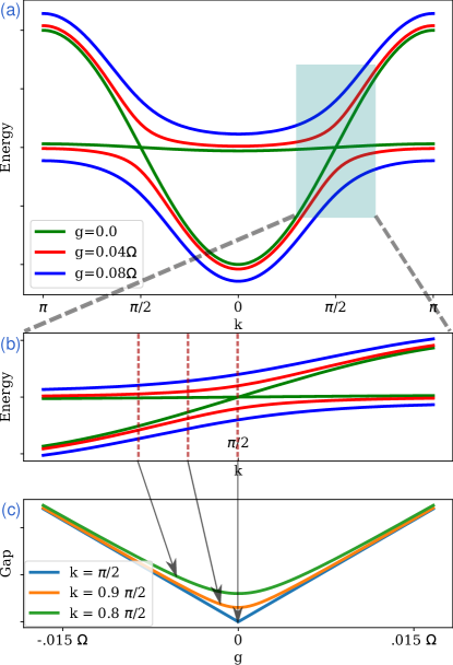
Figure 2: Bandstructure of the optomechanical array for detuning $\Delta=-\Omega$, (a) shows the energy of the modes versus $k$, with different colors denoting different values of the laser-tunable optomechanical coupling, $g$. (b) shows a close-up view of the crossing point at $k=\pi/2$. For $g=0$ it is a full crossing whereas in the presence of optomechanical coupling, it turns to an avoided crossing. (c) Shows the gap as a function of the coupling $g$ for different values of $k$. For $k=\pi/2$ the gap fully closes at $g=0$.

Figure (2) illustrates the resulting band structures of the optomechanical array for $\Delta=-\Omega$. The first term in equation (6) is proportional to Identity and only shifts the band structure. If we ignore the first term, for the regime of $\Delta=-\Omega$, the Hamiltonian of the system is

$$h_{k}=\left(J-K\right)\cos\left(k\right)\sigma_{z}+g\sigma_{x}.$$ (8)

Figure (2) shows how the spectrum and also the energy gap between the two modes depend on the value of $k$. For $k=0$, this gap is the largest and the gap is minimal at $k=\frac{\pi}{2}$. In the absence of optomechanical coupling, when $g=0$, the phononic band is almost flat and there are two crossings where the gap fully closes. In the presence of optomechanical coupling, $\left|g\right|>0$, the two bands do not cross. Far from the crossing points and in the middle, mode $\hat{A}_{k}$ is mostly phononic and outside, it is mostly photonic. Similarly, mode $\hat{B}_{k}$ is dominated by the photonic mode for $-\pi/2\leq k\leq\pi/2$ and by phononic modes outside this range.

From Eq. (8), the gap between the two bands can be calculated as

$$\Delta_{g}=2\sqrt{g^{2}+\cos\left(k\right)^{2}\left(J-K\right)^{2}}.$$ (9)

Here we are interested in the dynamical behaviour of the modes and their population as the Hamiltonian evolves. We focus on changing the optomechanical coupling. This is done via changing the driving power of the laser and, at each given value of k, takes the Hamiltonian through an avoided crossing (crossing if $k=\frac{\pi}{2}$) and could drive the system out of equilibrium.

We investigate the excitations from the mode $\hat{A}_{k}$ to the mode $\hat{B}_{k}$ as the Hamiltonian evolves through the avoided crossing.

II.1.2 Quench

We change the coupling $g$ according to

$$g\left(t\right)=g\left(0\right)(1-\frac{2t}{\tau_{Q}}),$$ (10)

where $\tau_{Q}$ represents the quench time and describes how fast the change is applied to the Hamiltonian. This can be set for instance by the rate at which the external laser changes in an experimental setting. The quench dynamics proceeds from $t=0$ to $t=\tau_{Q}$, switching the sign of the coupling from $+g(0)$ to $-g(0)$. Large $\tau_{Q}$ describes a slow change and adiabatic evolution and low $\tau_{Q}$ describes a more abrupt evolution. We set the time $t$ to start from zero and to go to $\tau_{Q}$. This makes the Hamiltonian time dependent.

The range of the time $\tau_{Q}$ should be set by the band gap in the system in Eq. (9), i.e. for $\tau_{Q}>\frac{g}{\Delta_{(g=0)}^{2}}$ the evolution would be adiabatic. This limit depends on the value of $k$, which means that a specific rate, $1/\tau_{Q}$, could be adiabatic for some values of $k$ and non-adiabatic for the rest of the range. For instance, for $k=\frac{\pi}{2}$, the gap fully closes and no matter how large the $\tau_{Q}$ is, the evolution cannot be adiabatic.

With the time evolution of the optomechanical coupling, the normal modes would also become time dependent. To avoid confusion with the time evolution of the modes, we refer to the normal modes with respect to their corresponding value of $g$, namely $\{\hat{A}_{k,g},\hat{B}_{k,g}\}$ which are calculated from the eigenvectors of $h_{k}(g)$ and

$$\left(\begin{array}[]{c}\hat{A}_{k,g}\\ \hat{B}_{k,g}\end{array}\right)=R_{k}(g)\left(\begin{array}[]{c}\hat{a}_{k}\\ \hat{b}_{k}\end{array}\right)$$ (11)

II.1.3 Time evolution

We use the equation of motions for $\{\hat{a}_{k}(t),\hat{b}_{k}(t)\}$ to find the time propagator of the evolution. We break down the evolution to small enough time-steps. The Hamiltonian should stay constant over the time-step (compared to $\|h_{k}(t)\|$). Then the time propagator is specified with

$$\frac{dS_{k}(t)}{dt}=-ih_{k}(t)S_{k}(t)$$ (12)

with the initial condition $S_{k}(0)=\mathcal{I}$ and $h_{k}$ is the Hamiltonian in Eq. (5) and $\delta t$ is the time step. Note that $\delta t\ll 1/\sqrt{\|\left[h_{k}(t),h_{k}(t+\delta t)\right]\|}$.

The operator $S_{k}(t)$ gives the evolution of the original modes $\{\hat{a}_{k},\hat{b}_{k}\}$ as

$$\left(\begin{array}[]{c}\hat{a}_{k}(t)\\ \hat{b}_{k}(t)\end{array}\right)=S_{k}\left(t\right)\left(\begin{array}[]{c}\hat{a}_{k}\\ \hat{b}_{k}\end{array}\right).$$ (13)

Now we can calculate the evolution of the normal modes too, which is given by

$$\left(\begin{array}[]{c}\hat{A}_{k,g(t)}\left(t\right)\\ \hat{B}_{k,g(t)}\left(t\right)\end{array}\right)=R_{k}(g(t))S_{k}\left(t\right)\left(\begin{array}[]{c}\hat{a}_{k}\\ \hat{b}_{k}\end{array}\right).$$ (14)

(See the SM for more details. )

Next we need to specify the initial state. Each mode could be populated with multiple excitations and therefore just knowing the evolution of the modes is not enough to track the excitations.

II.1.4 Initial state

One simple choice is to start with a single excitation in one of the normal modes. It however would be challenging to create a single excitation with a specific momentum experimentally. Probably the more realistic state to start with is the thermal state. This is the stationary state of the optomechanical array. More specifically, we assume that before we start changing the Hamiltonian, the system has enough time to reach its equilibrium with its environment. The normal mode populations of the stationary state are given by

$$n_{th}^{m}\left(\hat{A}_{k}\right)= \frac{\left(1-p_{k}\right)\Gamma n^{M}_{th}}{p_{k}\kappa+(1-p_{k})\Gamma}$$ (15)

$$n_{th}^{m}\left(\hat{B}_{k}\right)= \frac{p_{k}\Gamma n^{M}_{th}}{(1-p_{k})\kappa+p_{k}\Gamma}.$$ (16)

where $p_{k}$ is given by the projection of the normal mode $\hat{A}_{k}$ on the original mode $\hat{a}_{k}$.

Note that this is assuming that the optical bath is at zero temperature or equivalently, $k_{B}T\ll\hbar\omega_{optical}$. In this regime, we can scale the population of the two modes to $1/n_{th}^{M}$ as in Figure (3). For more details, see the SM.

II.1.5 Method

We initiate the system in the thermal state and let it evolve under the time dependent Hamiltonian. We probe the occupation number of the normal modes through the evolution, namely, we look at

$$\langle\psi(t)\mid\hat{A}_{k,g\left(t\right)}^{\dagger}\hat{A}_{k,g\left(t\right)}\mid\psi(t)\rangle$$

$$\langle\psi(t)\mid\hat{B}_{k,g\left(t\right)}^{\dagger}\hat{B}_{k,g\left(t\right)}\mid\psi(t)\rangle$$

See the SM for more details on how we calculate these quantities in our simulations.

II.2 Results

We start by comparing a fast and a slow quench. Figure (3) shows the simulation results for the final excitations for a slow, mid-speed and a fast quench. The top plot shows the results for excitations in mode A and the bottom one shows the excitations in mode B. For comparison, we included the initial population given by Eq. (15). It is critical to take these initial excitations into account when we study the excitations generated by the quench. Figure (3) also shows that for a slow quench, the number of excitations stays almost unchanged, whereas for the fast quench, new excitations are generated through the quench process.

Figure 3: Quench dynamics for a quench from positive to negative coupling ($g\left(0\right)$ to $-g\left(0\right)$). (a) shows how the population changes through the quench for $k\approx.2\pi$ and some medium speed quench. (b) and (c) show the final population scaled to the thermal population of the bath, $N_{f}/n_{th}^{M}$, of mode $A$ (upper branch) and likewise mode B (lower branch) after a slow, medium-speed and fast quench. For the slow, medium and fast quench, $\frac{\tau_{Q}}{g(0)/\Delta_{g=0}^{2}}\approx.0001,.01,1$ respectively. The initial population $N_{i}$ is also included for comparison. The initial population $N_{i}$ is calculated based on the thermal equilibrium state with a bath and the final population is derived evolving the initial state while changing the Hamiltonian. Depending on the rate at which the Hamiltonian changes, the overall evolution can be non-adiabatic or adiabatic. For the slow quench, the final population, $N_{f}$, is close to the initial one, however for the fast and mid-speed quenches, the evolution generates some excitations. The band structure and the gap between the two bands depends on $k$, so the final populations $N_{f}$ would also depend on $k$. For instance the gap closes for $k=\pi/2$ and both modes would have the same energy, so no matter how slow we quench the Hamiltonian, in the vicinity of this point, the evolution would always be non-adiabatic and the value of $N_{f}$ would increase.

Provided we assume $\Delta=-\Omega$ (as we will do for these simulation), the gap between the two bands, $\Delta_{g}$, vanishes for $k=\pi/2$ (See Eq. (9) and figure (2)) and as a result, the dynamics is always non-adiabatic at this point. This explains why there are excitations generated in the vicinity of $k=\pm\pi/2$, even for the slow quench.

Here we focus on the net excitation, $N_{Q}$ which is

$$N_{Q}=N_{f}-N_{i},$$ (17)

where $N_{f}$ and $N_{i}$ represent the final and initial population of the bands.

Figure (4) shows the net excitations in mode A for different quench times, $\tau_{Q}$. This figure indicates that there is a regime for which the dynamics is non-adiabatic. We introduce $k_{c}$ to indicate the range of the non-adiabatic regime. We define $k_{c}$ as the maximum distance from $k=\frac{\pi}{2}$ where the excitation generated by the quench, $N_{Q}$, is above some threshold $\epsilon$. Note that there are two non-adiabatic regions, one around $k=\frac{\pi}{2}$ and one for $k=\frac{-\pi}{2}$ We only consider the region around $k=\frac{\pi}{2}$ for simplicity and restrict our discussion to positive values of $k$. Mathematically, that is $k_{c}=\min\{p\mid\forall k\mid k-\pi/2\mid>p,N_{Q}\left(k\right)<\epsilon\}$ where $\epsilon$ is some threshold. The parameter $k_{c}$ is mostly affected by the quench time $\tau_{Q}$.

Figure 4: Net excitation in mode A for different quench times, $\tau_{Q}$. Different plots represent different quench times. From the top to the bottom, $\tau_{Q}$ increases. For the slow, medium, fast and very fast quench, $\frac{\tau_{Q}}{g(0)/\Delta^{2}_{g=0}}\approx.03,.01,.001,.0001$ respectively. This indicates that the slower the quench, the less excitation would be generated and the smaller the non-adiabatic regime would be. (b) shows a close-up view of the plot in (a) around $k=\pi/2$, where the gap closes. This indicates that even for slower quenches, there are some excitations around the level-crossing point. For the simulations here we used $\Delta=-\Omega,g=0.02\Omega,\kappa=0.01\Omega,\Gamma=0.001\Omega$. See the text for more details.

Figure (5) shows $k_{c}$ as a function of the quench time, $\tau_{Q}$. This plot shows the power-law dependence of the size of the non-adiabatic regime, $k_{c}$, on the quench time.

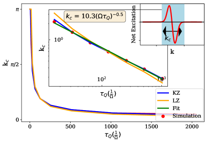
Figure 5: The extent of the non-adiabatic regime, $k_{c}$, as a function of quench time, $\tau_{Q}$. This plot illustrates a power-law dependence on the quench time. We included the two analytical estimates along the best linear fit for the simulation results which are in good agreement. The first analytic estimate comes from the Landau-Zener formula. The second one is adopted based on the Kibble-Zurek mechanism. See section (II.3). The fit and its corresponding equation are included in the log-log plot in the inset in the middle. Note that fit is expected to give $k_{c}\approx\frac{\sqrt{2g(0)}}{(J-K)\sqrt{\pi\tau_{Q}}}$, that is mostly affected by the values of $g(0)$ and $J$ and for the parameters here gives $k_{c}\approx\frac{10}{\sqrt{\tau_{Q}}}$ The top-right inset shows the non-adiabatic regime in the net excitation plot from figure(4-b).

For these simulations, we take the following values for the quench time

$$\tau_{Q}\in\frac{50}{\Omega}\times\{2^{-1},2^{0},2^{1},\cdots,2^{10}\}.$$

These values are set such that the smallest value would give a non-adiabatic evolution for all values of $k$ and the largest value would give an adiabatic evolution for essentially all the values of $k$ that we consider in our simulations.

Next we will assess the dynamics analytically and show that these results are compatible with analytical expectations.

II.3 Analytical assessment

The simulation results here can be approximated with the Landau-Zener (LZ) formula for excitations in a time-dependent two-level system. For a two-level system with $\left(h_{k}\right)_{12}=(J-K)cos(k)$ as the off-diagonal elements of the Hamiltonian, the Landau-Zener formula Zener (1932); Landau and Lifshitz (1958) gives the probability of excitation as

$$P_{LZ}=e^{\frac{\pi\left(J-K\right)^{2}}{2g\left(0\right)}\cos\left(k\right)^{2}\tau_{Q}}.$$ (18)

Note that we used the Hamiltonian in Eq. (8) to calculate the probability. This shows that the border between the adiabatic and non-adiabatic regime is approximately given by $\tau_{Q}\approx 2g\left(0\right)/\pi\left(K-J\right)^{2}\cos\left(k\right)^{2}$, i.e. if the quench happens on a faster time-scale, then the evolution would be non-adiabatic and generates excitations and similarly, if it is slow, then the evolution would be adiabatic and gives no extra excitations.

If we expand this in terms of small $\delta k$ from $\pi/2$, we have $\cos\left(\pi/2+\delta k\right)=\sin\left(\delta k\right)\approx\delta k$ and we get $k_{c}\approx\frac{\sqrt{2g(0)}}{(J-K)\sqrt{\pi\tau_{Q}}}$, which indicates that the size of the non-adiabatic region in k space, $k_{c}$, has a power-law dependence on the quench time, $\tau_{Q}$. The Landau-Zener fit is included in Figure (5) for comparison and confirms the simulation results.

A more intuitive approach is to break down the evolution into two phases, the adiabatic and freeze-out zone. This is similar to the Kibble-Zurek mechanism (KZ) Kibble (1976); Zurek (1985, 1996); Nalbach et al. (2015).

We assume that the dynamics in the adiabatic zone is fully adiabatic. Similarly, we assume that the state does not change in the freeze-out zone. Clearly, this is an approximation and the transition from adiabatic to non-adiabatic dynamics is usually gradual and the state does not fully freeze. However, this gives a good fit to our numerical simulations.

Assume that the evolution starts in $t_{i}=-\infty$ with the coupling $g(t_{i}=-\infty)=-g_{m}$ and goes to $t_{f}=\infty$ with coupling $g(t_{f}=\infty)=g_{m}$, and that we start with the ground state. We use the $\{\left|G(t)\right\rangle,\left|E(t)\right\rangle\}$ to represent the ground and excited states of the Hamiltonian at time $t$. This is not to be confused with the optomechanical coupling $g\left(t\right)$. Note that, for simplicity, we are taking time to symmetrically evolve from $-\infty$ to $\infty$ which is slightly different from our convention in Eq. (10), but it does not change the result and it can be easily transformed to the convention in Eq. (10).

More importantly, we assume that at some time, $-\hat{t}$, the evolution transits from adiabatic to the freeze-out zone and then becomes adiabatic again at $\hat{t}$. Under these assumptions, the state evolves as follows

$$\left|\psi_{i}\right\rangle =\mid G\left(-\infty\right)\rangle\rightarrow\left|\psi\left(-\hat{t}\right)\right\rangle\approx\mid G\left(-\hat{t}\right)\rangle\rightarrow$$

$$\left|\psi\left(\hat{t}\right)\right\rangle \approx\mid G\left(-\hat{t}\right)\rangle=\alpha\mid G\left(\hat{t}\right)\rangle+\beta\mid E\left(\hat{t}\right)\rangle$$

$$\rightarrow \left|\psi_{f}\left(\hat{t}\right)\right\rangle\approx\alpha\mid G\left(\infty\right)\rangle+\beta\mid E\left(\infty\right)\rangle.$$

First, we start with the state at $t=-\infty$. Up to $t=-\hat{t}$ the evolution is adiabatic which keeps the state in the ground state. From this point, up to $t=\hat{t}$ the state freezes and stays unchanged. So at time $t=\hat{t}$, we still have the $\left|G(-\hat{t})\right\rangle$, which no longer represents the ground state, but some superposition of both the ground and excited states. Beyond this, the evolution is adiabatic again which preserves the superposition.

Therefore, the amount of excitations are given by $\left|\beta\right|^{2}$. In order to calculate $\beta$, we only need to know the projection of eigenstates at $-\hat{t}$ to the eigenstates at $\hat{t}$.

The eigenvectors of the optomechanical array can be calculated from Eq. (8) and would give

$$\mid\beta\mid^{2}=\frac{\left(g_{m}\frac{\hat{t}}{\tau_{q}}\right)^{2}}{\left(g_{m}\frac{\hat{t}}{\tau_{q}}\right)^{2}+\delta^{2}}.$$ (19)

Next we need to find $\hat{t}$. If we follow the same idea as in the Kibble-Zurek mechanism, this is the time at which it takes the same amount of time for the system to relax as it has to get to the crossing point, i.e. $\hat{t}=\tau_{\text{relx}}=\frac{1}{\sqrt{\delta^{2}+\left(g_{m}\frac{\hat{t}}{\tau_{q}}\right)^{2}}}$, with $\tau_{\text{relx}}$ the relaxation time. Note that this is not an actual relaxation time, but the time scale given by the $\frac{1}{\text{Gap}}$.

If we plug this into Eq. (19), we get

$$\beta=1-\frac{2\delta^{2}\text{$\tau_{q}$}^{2}}{\delta^{2}\text{$\tau_{q}$}^{2}+\sqrt{\delta^{4}\text{$\tau_{q}$}^{4}+32g^{2}\tau_{q}^{2}}}.$$ (20)

The KZ analytical fit is also included in figure (5) which shows that both analytical assessments are in good agreement with the simulation results.

This concludes the results in this section. We studied the excitations generated through the quench and showed that they are compatible with KZ and LZ predictions.

II.4 Experimental Imperfections

Now we investigate the experimental challenges of implementing and testing our results.

As we stated before, we assume that we are working in the strong coupling regime, i.e. $g\gg\kappa$. This has already been achieved experimentally in Teufel et al. (2011b); Gröblacher et al. (2009).

We also ignored the dissipation for the most part, but we can also extend our simulation to the situation where the dissipation is not ignored. Figure (6) shows how the typical behaviour of this system changes as we add dissipation. Without dissipation, the gray plots show how evolving the Hamiltonian through the avoided crossing would swap the populations of the two modes. However, when dissipation is included, both populations start to decline to a point that if the quench is not fast enough, they would not cross. Figure (6) shows how dissipation would affect the net excitation generated through the dynamics. Although the general trend is preserved, the net excitation is decreased compared to the one in figure (4). Note that here we assume that the photonic bath is at zero temperature which is consistent, considering that typically $\hbar\omega_{\text{Optical}}\gg k_{b}T$, with $\omega_{\text{Optical}}$ the optical frequency. We also assume that $\Gamma\ll\kappa,g$ for this plot which can be fulfilled in most experiments.

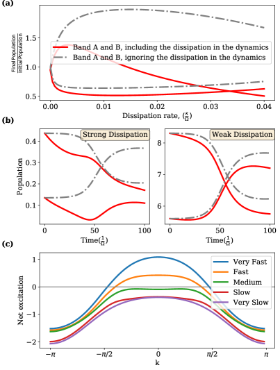
Figure 6: The influence of dissipation on the evolution and final population of the modes. (a) shows how the final population of the two modes would be affected in the presence of dissipation. To give a reference for comparison, the results in the absence of dissipation are also included. Dissipation reduces the final population. Note that, since for different amounts of dissipation, the initial population changes, the results are normalized to the initial values for each point. Plots in (b) illustrate how the dissipation affects the dynamics of the populations. Line colors and styles are the same as the ones in (a). In each plot, the population of the two modes A and B, both in the presence and absence of dissipation, are shown versus time, as the system evolves through the avoided crossing. For the plot on the right, the quench is still fast enough for the two populations to cross, however, for stronger dissipation, the population of both bands could decay before the can cross. (c) shows the net excitation generated through the evolution in the presence of dissipation. The general trend is similar to the one in figure (4), however, due to the dissipation, the net excitation has dropped. Different plots corresponds to different quench times. For the very slow, slow, medium, fast and very fast quench, $\frac{\tau_{Q}}{g(0)/\Delta^{2}_{g=0}}\approx.03.015,.007,.0005,.0001$ respectively.

In all the illustrations so far, we assumed $\Delta=-\Omega$ (red detuned regime) and all the mode dynamics to be described by the beam-splitter Hamiltonian (which relies on $J,K<<\Omega$). I n principle, one can consider arbitrary detunings, including those where excitations may be generated by the amplification terms in the Hamiltonian.

One of the main challenges in analysing a regime including photon-phonon pair generation would be that it is not possible to distinguish the excitations that are generated directly by the parametric terms from the ones generated by the quench. This explains why we focus on the regime where number-non-preserving terms in the Hamiltonian are suppressed and all the excitations can be associated to the quench.

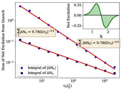
Figure 7: This plot shows the sum of all excitations with different momenta as a function of the quench time. The circles show the sum of the absolute values of the net excitations and the squares show the sum, i.e. the integral under the plots in figure (4) for different quench times. The red curves give the best linear fit to the data points. The equations of the fits are included next to the plots. The inset shows the net population after the quench around $k=\frac{\pi}{2}$. See figure (4-b) for more details

Another challenge is that for the results in figure (4), excitations with different pseudo-momentum should be resolved. While this is in principle possible Schmidt et al. (2013), a simpler solution is to look at the sum of the net excitations, i.e. $\int N_{Q}\left(k\right)dk$. This is the area under the plot of $N_{Q}\left(k\right)$. Figure (7) shows this quantity for different quench times. Although the net exitations still follow a power-law, the values are too small and probably challenging to detect experimentally. Alternatively, we can investigate the absolute value of the net excitation, which still gives a power-law, but this would require $k$-resolved measurements of the excitations too.

The last assumption that needs clarification is the periodic boundary conditions on the lattice, which makes it possible to work in Fourier space. It is possible to do this calculations for a finite-size system and work out the excitations for different sites on the lattice, but it is computationally more challenging.

III Application: Quenches in the Optomechanical Su-Schrieffer-Heeger  model

So far, the main focus has been to understand how changes in the Hamiltonian would affect the dynamics of optomechanical arrays. In this section we will give an example to illustrate how optomechanical arrays can be designed to mimic the evolution of the SSH model. This model exhibits a topological phase transition, which makes it a nice candidate for exploiting the dynamical properties of the optomechanical array for simulation purposes.

The SSH model describes a one-D topological insulator Asbóth et al. (2016) where fermions can hop from one site to the other, however, hopping rates are staggered and the hopping rate to the left and right are different for each site. See figure (8) for a schematic picture of the SSH model. The SSH model has two phases that are separated by a topological phase transition. For the finite size model, one phase exhibits zero-energy edge states.

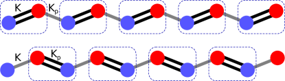
Figure 8: Schematic picture of the SSH model. The two figures illustrate the two phases of the model, the top one is when $K$ is the dominant coupling and bottom is revered. For the latter, in contrast to the top one, not all the sites can pair up and two sites are left at the two ends of the lattice which produce the zero-energy edge states.

Here we first present a brief introduction to the SSH model and then propose an optomechanical array design that emulates the SSH model and show how the effective dynamics is compatible with SSH.

III.1 SSH model

For the purposes of this work, it suffices to understand the Hamiltonian and the phase diagram of the SSH model. This model comprises a chain that can be separated into two distinct sublattices. We refer to these sublattices as sublattice A and B. Fermions on each sublattice have similar right and left hopping rates. This means

$$H_{SSH}=K\sum_{i=1}^{N}\left(\hat{c}_{i}^{\dagger}\hat{d}_{i}+\hat{c}_{i}\hat{d}_{i}^{\dagger}\right)+K_{p}\sum_{i=1}^{N-1}\left(\hat{c}_{i+1}^{\dagger}\hat{d}_{i}+\hat{c}_{i+1}\hat{d}_{i}^{\dagger}\right),$$ (21)

where $\hat{c}_{i}$ and $\hat{d}_{i}$ are the annihilation operators on odd and even sites, corresponding to the two sublattices. Note that to avoid confusion with the creation operators for the photonic and phononic modes in the first part of the paper, we use $\hat{c}_{i}$ and $\hat{d}_{i}$ here.

Here we assume a finite-size lattice with $2N$ sites.

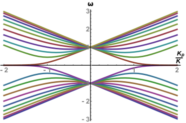
Figure 9: The spectrum of the finite-size SSH model with 20 sites and 10 unit cells as a function of the ratio of the hopping rates $\{K,K_{p}\}$. For $|K_{p}|>|K|$ two energy levels start to converge and form the two zero-energy edge states.

The spectrum of the SSH model with 20 sites (10 unit cells) is shown in figure (9). Each line represents one energy level and the plot shows how energy levels change with the ratio of the hopping rates. This model has two phases which are distinguished by the order parameter $\lambda=K_{p}/K$. For $\lambda<1$, all the sites pair up and form dimers. In the opposite regime, i.e. $\lambda>1$, all the particles in the middle pair up, however, there are two sites left out at the two ends. These two make the two zero-energy edge states of the SSH model. These are the two energy levels at zero energy in figure (9) which form beyond $\lambda=1$. These dimers are shown schematically with dashed rectangles for the two phases in figure (8). For a detailed introduction of this model see Su et al. (1979); Asbóth et al. (2016).

Here we first show how an optomechanical array can be tuned to mimic the SSH model. Then we use the dynamical tunability of the optomechanical system to change the order parameter and emulate the topological phase transition in the SSH model and drive the system out of equilibrium.

It is important to note that here a modified SSH model is being simulated, namely a bosonic SSH model instead of the fermionic one. However, the phase transition in question only relates to the properties of the single particle wave functions, and hence does not depend on whether we are dealing with fermions or bosons.

Next we give the design for the simulator and explain the intuition behind it. We then present a detailed calculation of the effective Hamiltonian and show that the Hamiltonian of the simulator is compatible with the SSH model.

III.2 Proposal for simulator

A schematic picture of our design for the optomechanical simulator is given in figure (10). Such a design can potentially be implemented in optomechanical crystals Safavi-Naeini et al. (2014) and electromechanical arrays Lecocq et al. (2015).

Figure 10: Schematic of the simulator. Blue/Yellow circles indicate optical/mechanical modes. The mechanical modes in each cell are indirectly coupled through their coupling to the coupled optical modes. This coupling can be tuned using an external laser that tunes the optomechanical coupling, $g$.

We use the mechanical modes as the main modes of the SSH model. There are two kinds of coupling between the mechanical modes: there is the direct coupling, $K$, through the vibrations on the substrate and the indirect one through the coupling to the optical modes. The indirect coupling depends on the direct optical coupling rate, $J$, and the optomechanical coupling rate, $g$.

Next, we calculate the effective Hamiltonian of the array in figure (10) and find the indirect coupling with second order perturbation theory.

III.3 Effective Hamiltonian

To find the effective Hamiltonian, we focus on one unit cell which includes two connected optomechanical nodes (first half of the figure (10)). The Hamiltonian of the unit cell is given by

$$\hat{H} =\sum_{i}\left(-\hbar\Delta\hat{a}_{i}^{\dagger}\hat{a}_{i}+\hbar\Omega\hat{b}_{i}^{\dagger}\hat{b}_{i}\right)$$

$$-\hbar g\sum_{i}\left(\hat{a}_{i}^{\dagger}\hat{b}_{i}+\hat{a}_{i}\hat{b}_{i}^{\dagger}\right)$$

$$+\hbar J\sum_{{\rm odd}\,i}\left(\hat{a}_{i}^{\dagger}\hat{a}_{i+1}+\hat{a}_{i}\hat{a}_{i+1}^{\dagger}\right)$$

$$+\hbar K\sum_{{\rm even}\,i}\left(\hat{b}_{i}^{\dagger}\hat{b}_{i+1}+\hat{b}_{i}\hat{b}_{i+1}^{\dagger}\right).$$

We block-diagonalize the subspace corresponding to the photonic bands and transform the Hamiltonian into a basis that instead of the original optical modes, is expressed in terms of the normal modes of the coupled optical cavities. These normal modes are the symmetric and anti-symmetric superposition of the original photonic modes, i.e.

$$\hat{A}_{\pm}=\frac{\hat{a}_{1}\pm\hat{a}_{2}}{\sqrt{2}}.$$ (22)

For a unit cell, this gives

$$\hat{H} =-\hbar\Delta\left(\hat{A}_{+}^{\dagger}\hat{A}_{+}+\hat{A}_{-}^{\dagger}\hat{A}_{-}\right)$$

$$+\hbar\Omega\left(\hat{b}_{1}^{\dagger}\hat{b}_{1}+\hat{b}_{2}^{\dagger}\hat{b}_{2}\right)$$

$$-\frac{\hbar g}{\sqrt{2}}\left(\hat{A}_{+}^{\dagger}\left(\hat{b}_{1}+\hat{b}_{2}\right)+\hat{A}_{-}^{\dagger}\left(\hat{b}_{1}-\hat{b}_{2}\right)+h.c.\right)$$

$$+\hbar J\left(\hat{A}_{+}^{\dagger}\hat{A}_{+}-\hat{A}_{-}^{\dagger}\hat{A}_{-}\right).$$

Note that there are couplings between the mechanical modes in the unit cell and the neighbouring cells which are not included in the Hamiltonian of the unit cell. We will later include them as interaction terms between different cells.

The symmetric and anti-symmetric photonic modes couple to both mechanical modes. We use the Bloch matrix of the Hamiltonian above to calculate the indirect coupling between the two mechanical modes with second order perturbation theory, which gives

$$\hat{H} =\hbar\hat{\Omega}\sum_{i}\left(\hat{b}_{i}^{\dagger}\hat{b}_{i}\right)$$

$$+\hbar K_{p}\sum_{{\rm odd}\,i}\left(\hat{b}_{i}^{\dagger}\hat{b}_{i+1}+\hat{b}_{i}\hat{b}_{i+1}^{\dagger}\right)$$

$$+\hbar K\sum_{{\rm even}\,i}\left(b_{i}^{\dagger}b_{i+1}+b_{i}b_{i+1}^{\dagger}\right),$$

where $K_{p}$ is the effective coupling in the SSH model and is

$$K_{p}=\frac{2g^{2}J\left(-\Delta^{2}+J^{2}-\Omega^{2}\right)}{(-\Delta+J-\Omega)(\Delta+J-\Omega)(-\Delta+J+\Omega)(\Delta+J+\Omega)}$$

Note that this can be tuned with $g$. Using the parameters that we used for the first part, the couplings in the SSH model can be estimated as $K=3MHz,K_{p}=10MHz$.

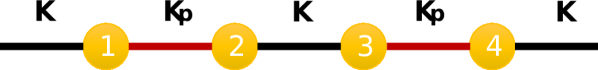
Figure 11: Effective model after applying second-order perturbation theory to the optomechanical array of figure (10).

The coupling $K_{p}$ depends on the optomechanical coupling $g$. The above numerical estimate for $K_{p}$ is the maximum that can be achieved using the parameters that we considered here. Reducing the laser power, it can be tuned to $K_{p}<K$ which changes the phase to the non-topological phase.

This can be used to explore a wide range of properties in this system. For instance, we can start in the topological phase with $\lambda>1$, with the system initialized in one of the edge states and then abruptly change the Hamiltonian to the non-topological phase with $\lambda<1$ and probe the evolution of the edge states.

Figure (12) shows the dynamics of the excitations in this system as it evolves through time and space. The excitation on the left side of the chain starts to propagate to the right after the quench. Figure (12-b) shows one slice of figure (12-a) which represents the probability of observing the excitation on the right side of the lattice after time $t$. This probability is negligible at first, and it increases after the initially produced excitations have travelled through the whole lattice.

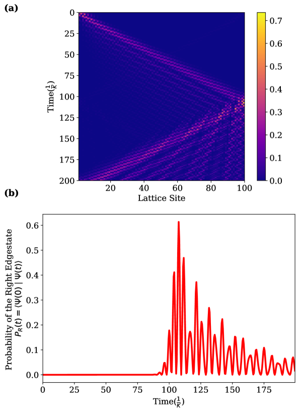
Figure 12: Time evolution of an excitation in the SSH model, initiated on the left side of the lattice, while abruptly quenching the Hamiltonian to the non-topological phase. Plot (a) shows the propagation of the left edge state in time and space (lattice site). Plot (b) shows the probability of getting the right edge state in time, i.e. $P_{R}(t)=|\langle\Psi(t=0)\left|\Psi(t=t)\right\rangle|^{2}$. At time $t=0$, the excitation is on the leftmost site of the lattice and it starts travelling to the right. For this simulations, we started with Hamiltonian in the topological phase and the left edge state for the $\left|\Psi(t=0)\right\rangle$. After the quench to the non-topological phase, it takes some time for the excitation to reach the right side of the lattice. The plot (b) corresponds to the last site of the lattice of (a), indicated in the red box.

IV Conclusion

We have studied non-equilibrium effects in optomechanical arrays which can be caused by abrupt changes in the parameters of the system, induced via the driving laser. We have analyzed the resulting excitations and we have shown that the number of such excitations follows a power law with respect to the quench speed.

We have also provided a proposal for exploiting the dynamical aspects of optomechanical arrays for simulating non-equilibrium dynamics in the SSH model, as a simple example of an array with a band structure that has topological properties.

We have commented on the experimental outlook. Still, to adopt the first results presented here for concrete experimental platforms, some further, more detailed analysis will be needed. For example, the effects of disorder Roque et al. (2017) may need careful additional consideration.

More generally, the present work paves the way towards investigating other aspects of non-equilibrium dynamics in optomechanical arrays with time-dependent band structures. Further studies may reveal which other kinds of phenomena should be expected and tested in these settings. We emphasize that the optomechanical system we have considered here is in the linear regime, with a quadratic Hamiltonian, and is not capable of capturing the complexity of quantum simulation of non-trivial quantum many-body systems. Yet, as we have shown, even the linear dynamics displays a rich set of features. In the near-term future, one might also study the nonlinear classical dynamics in nonequilibrium optomechanical arrays, which is perfectly within experimental reach.

We thank Vittorio Peano for fruitful discussions. This work was supported by the ERC Starting Grant OPTOMECH. This work is supported by the research grant system of Sharif University of Technology (G960219), the European Union’s Horizon 2020 research and innovation programme under grant agreement No 732894 (FET-Proactive HOT).

Normal modes

Here we give an expression for the normal modes of the Hamiltonian.

The normal modes are given by the eigenvectors of the $h_{k}$. To find the eigenvectors, it helps to rewrite it as

$$h_{k}=\frac{\Omega(k)-\Delta(k)}{2}\mathbb{{1}}-\frac{\Omega(k)+\Delta(k)}{2}\sigma_{z}+g\sigma_{x}.$$ (S1)

Here $\sigma_{i}$ are the Pauli operators. The first term does not affect the eigenvectors. So the eigenvectors are the eigenvectors of a rotated Pauli operator in the $x-z$ plane. With a simple rotation, we can transform the eigenvectors of $\sigma_{z}$ to the eigenvectors of the rotated Pauli operator. For simplicity, we define $2\delta(k)=\Omega(k)+\Delta(k)$. With some simple algebra we get to

$$\vec{\lambda}_{\pm}\left(k\right)=\frac{1}{z_{\pm}}\left(\begin{array}[]{c}-g\pm\sqrt{g^{2}+\delta\left(k\right)^{2}}\\ \delta\left(k\right)\end{array}\right),$$ (S2)

with $z_{\pm}$ the normalization factors. Now if we apply the transformation that diagonalizes the $h_{k}$, we get

$$\hat{H}_{OMA}= \sum_{k}\hbar\left(\begin{array}[]{cc}\hat{a}_{k}^{\dagger}&\hat{b}_{k}^{\dagger}\end{array}\right)\left(\begin{array}[]{cc}-\Delta\left(k\right)&g\\ g&\Omega\left(k\right)\end{array}\right)\left(\begin{array}[]{c}\hat{a}_{k}\\ \hat{b}_{k}\end{array}\right)$$

$$= \sum_{k}\hbar\left(\begin{array}[]{cc}\hat{a}_{k}^{\dagger}&\hat{b}_{k}^{\dagger}\end{array}\right)R_{k}^{\dagger}\left(\begin{array}[]{cc}\omega_{A}\left(k\right)&0\\ o&\omega_{B}\left(k\right)\end{array}\right)R_{k}\left(\begin{array}[]{c}\hat{a}_{k}\\ \hat{b}_{k}\end{array}\right)$$

$$= \sum_{k}\hbar\left(\begin{array}[]{cc}\hat{A}_{k}^{\dagger}&\hat{B}_{k}^{\dagger}\end{array}\right)\left(\begin{array}[]{cc}\omega_{A}\left(k\right)&0\\ o&\omega_{B}\left(k\right)\end{array}\right)\left(\begin{array}[]{c}\hat{A}_{k}\\ \hat{B}_{k}\end{array}\right)$$

$$= \sum_{k}\hbar\left(\omega_{A}\left(k\right)\hat{A}_{k}^{\dagger}\hat{A}_{k}+\omega_{B}\left(k\right)\hat{B}_{k}^{\dagger}\hat{B}_{k}\right).$$

Here $\left\{\omega_{A}\left(k\right),\omega_{B}\left(k\right)\right\}$ are the eigenvalues of the $h_{k}$ and $R_{k}$ is the matrix that diagonalizes it. You can see that it gives the transformation in Eq. (4) in the main text.

Initial state population

We need to find the equilibrium population of the normal modes. For $g=0$ or too far off resonance, the normal modes are the same as the original modes, however, as we approach the avoided crossing points, the modes hybridize.

Before we get to the calculation of the equilibrium population of the normal modes, it helps to review the same calculation for the simple case of an isolated mechanical mode. The equation of motion for a single mechanical resonator is

$$\dot{\hat{b}}\left(t\right)=\left(-i\Omega-\Gamma/2\right)\hat{b}\left(t\right)+\sqrt{\Gamma}\hat{b}_{in}\left(t\right),$$

where $\hat{b}_{in}$ represents the annihilation operator of the mechanical bath modes. This is a simple differential equation which gives

$$\hat{b}\left(t\right)=e^{-i\Omega t-\Gamma t/2}\left(\hat{b}_{0}\left(t\right)+\sqrt{\Gamma}\int_{0}^{t}dt^{\prime}e^{i\Omega t^{\prime}+\Gamma t^{\prime}/2}\hat{b}_{in}\left(t\right)\right)$$

We are interested in $n^{m}=\langle\hat{b}^{\dagger}\left(t\right)\hat{b}\left(t\right)\rangle$ which is

$$n^{m}=\langle\hat{b}^{\dagger}\left(t\right)\hat{b}\left(t\right)\rangle=e^{-\Gamma t}\left(\langle\hat{b}_{0}^{\dagger}\left(t\right)\hat{b}_{0}\left(t\right)\rangle+\Gamma\int_{0}^{t}\int_{0}^{t}dt^{\prime}dt^{\prime\prime}e^{\Gamma(t^{\prime}+t^{\prime\prime})/2}e^{\Omega(t^{\prime}-t^{\prime\prime})}\langle\hat{b}_{in}^{\dagger}\left(t^{\prime}\right)\hat{b}_{in}\left(t^{\prime\prime}\right)\rangle\right).$$

We make the Markov approximation for the bath which implies that $\langle\hat{b}_{in}^{\dagger}\left(t^{\prime}\right)\hat{b}_{in}\left(t^{\prime\prime}\right)\rangle=\delta\left(t^{\prime}-t^{\prime\prime}\right)n_{th}^{m}$. This approximation simplifies the calculation and gives

$$n^{m} =e^{-\Gamma t}\left(n_{0}^{m}+n_{th}^{m}\Gamma\int_{0}^{t}dt^{\prime}e^{\Gamma t^{\prime}}\right)$$

$$=e^{-\Gamma t}\left(n_{0}^{m}+n_{th}^{m}\Gamma\frac{\left(e^{\Gamma t}-1\right)}{\Gamma}\right)$$

$$=e^{-\Gamma t}\left(n_{0}^{m}-n_{th}^{m}\right)+n_{th}^{m}.$$

For the stationary state, $t\rightarrow\infty$, we get $n^{m}\rightarrow n_{th}^{m}.$

Despite the simplicity, this calculation is the main tool we need to find the population of the normal modes in the stationary state.

Consider the equations of motion

$$\dot{\hat{X}}=M\cdot\hat{X}+\hat{\xi}\left(t\right),$$ (S3)

where $\hat{X}=\left(\begin{array}[]{c}\hat{a}\left(t\right)\\ \hat{b}\left(t\right)\end{array}\right),\,\xi=\left(\begin{array}[]{c}\sqrt{\kappa}\hat{a}_{in}\left(t\right)\\ \sqrt{\Gamma}\hat{b}_{in}\left(t\right)\end{array}\right)$ and

$$M=\left(\begin{array}[]{cc}i\Delta-\frac{k}{2}&ig\\ ig&-i\Omega-\frac{\Gamma}{2}\end{array}\right).$$ (S4)

Here we are ignoring the amplification terms in the Hamiltonian.

For the normal modes, we diagonalize $M$ without the dissipation terms.

This transforms the eq.(S3) to

$$d\left(\begin{array}[]{c}\hat{A}\left(t\right)\\ \hat{B}\left(t\right)\end{array}\right)/dt=\left(\begin{array}[]{cc}-i\omega_{A}+\frac{\kappa_{A}}{2}&0\\ 0&-i\omega_{B}+\frac{\kappa_{B}}{2}\end{array}\right)\cdot\left(\begin{array}[]{c}\hat{A}\left(t\right)\\ \hat{B}\left(t\right)\end{array}\right)+\left(\begin{array}[]{c}\hat{A}_{in}\left(t\right)\\ \hat{B}_{in}\left(t\right)\end{array}\right).$$

$\{\omega_{A},\omega_{B}\}$ are the frequencies of the normal modes and $\{\kappa_{A},\kappa_{B}\}$ are the dissipation corresponding to these modes. Also $\{\hat{A}_{in}\left(t\right),\hat{B}_{in}\left(t\right)\}$ are linear superpositions of $\hat{a}_{in}\left(t\right),\hat{b}_{in}\left(t\right)$. Note that $\{\kappa_{A},\kappa_{B}\}$ can be calculated as the first order perturbation to the $M$ without dissipation. More specifically we can take

$$M=\left(\begin{array}[]{cc}i\Delta&ig\\ ig&-i\Omega\end{array}\right)+\left(\begin{array}[]{cc}-\frac{\kappa}{2}&0\\ 0&-\frac{\Gamma}{2}\end{array}\right).$$ (S5)

Now if we focus on the population of the normal modes $\hat{A}$ and $\hat{B}$, it would be the same calculation that we did for an isolated mode, except for the fact that $\hat{A}_{in}$ and $\hat{B}_{in}$ are now affected by both the optical and mechanical baths. Repeating the calculations above, we get

$$\langle\hat{A}^{\dagger}\left(t\right)\hat{A}\left(t\right)\rangle=e^{-\kappa_{A}t}\left(\langle\hat{A}_{g\left(0\right)}^{\dagger}\left(t\right)\hat{A}_{g\left(0\right)}\left(t\right)\rangle+\int_{0}^{t}\int_{0}^{t}dt^{\prime}dt^{\prime\prime}e^{\kappa_{A}(t^{\prime}+t^{\prime\prime})/2}e^{\omega_{A}(t^{\prime}-t^{\prime\prime})}\langle\hat{A}_{in}^{\dagger}\left(t^{\prime}\right)\hat{A}_{in}\left(t^{\prime\prime}\right)\rangle\right)$$ (S6)

Now this requires the calculation of $\hat{A}_{in}(t)$ and $\hat{B}_{in}(t)$ which are given by the transformation $R$. In general

$$R=\left(\begin{array}[]{cc}\epsilon&\gamma\\ \mu&\nu\end{array}\right),\,\textrm{where }\epsilon^{2}+\gamma^{2}=1\,\textrm{and $\left|\epsilon\right|$=$\left|\nu\right|$ and $\left|\gamma\right|$=$\left|\mu\right|$.}$$

This transforms the modes as $\hat{A}_{in}\left(t\right)=\epsilon\sqrt{\kappa_{0}}\hat{a}_{in}\left(t\right)+\gamma\sqrt{\Gamma}\hat{b}_{in}\left(t\right)$ and $\hat{B}_{in}\left(t\right)=\mu\sqrt{\kappa_{0}}\hat{a}_{in}\left(t\right)+\nu\sqrt{\Gamma}\hat{b}_{in}\left(t\right)$ but more importantly,

$$\langle\hat{A}_{in}^{\dagger}\left(t\right)\hat{A}_{in}\left(t^{\prime}\right)\rangle= \epsilon^{2}\kappa_{0}\langle\hat{a}_{in}^{\dagger}\left(t\right)\hat{a}_{in}\left(t^{\prime}\right)\rangle+\gamma^{2}\Gamma\langle\hat{b}_{in}^{\dagger}\left(t\right)\hat{b}_{in}\left(t^{\prime}\right)\rangle$$

$$\langle\hat{B}_{in}^{\dagger}\left(t\right)\hat{B}_{in}\left(t^{\prime}\right)\rangle= \mu^{2}\kappa_{0}\langle\hat{a}_{in}^{\dagger}\left(t\right)\hat{a}_{in}\left(t^{\prime}\right)\rangle+\nu^{2}\Gamma\langle\hat{b}_{in}^{\dagger}\left(t\right)\hat{b}_{in}\left(t^{\prime}\right)\rangle.$$

Now recall that we are using the Markov approximation and since the optical bath is at zero temperature, we get

$$\langle\hat{A}^{\dagger}\left(t\right)\hat{A}\left(t\right)\rangle= e^{-\kappa_{A}t}\left(\langle\hat{A}_{g\left(0\right)}^{\dagger}\left(t\right)\hat{A}_{g\left(0\right)}\left(t\right)\rangle+\int_{0}^{t}\int_{0}^{t}dt^{\prime}dt^{\prime\prime}e^{\kappa_{A}(t^{\prime}+t^{\prime\prime})/2}e^{\omega_{A}(t^{\prime}-t^{\prime\prime})}\mid\gamma\mid^{2}\Gamma\delta\left(t^{\prime}-t^{\prime\prime}\right)n_{th}^{m}\right)$$

$$= e^{-\kappa_{A}t}\left(\langle\hat{A}_{g\left(0\right)}^{\dagger}\left(t\right)\hat{A}_{g\left(0\right)}\left(t\right)\rangle+\mid\gamma\mid^{2}\Gamma n_{th}^{m}\int_{g0}^{t}dt^{\prime}e^{\kappa_{A}t^{\prime}}\right)$$

$$= e^{-\kappa_{A}t}\left(\langle\hat{A}_{g\left(0\right)}^{\dagger}\left(t\right)\hat{A}_{g\left(0\right)}\left(t\right)\rangle+\mid\gamma\mid^{2}\Gamma n_{th}^{m}\left(\frac{e^{\kappa_{A}t}-1}{\kappa_{a}}\right)\right)$$

$$\left(\underset{t\rightarrow\infty}{\lim}\right)= \frac{\mid\gamma\mid^{2}\Gamma n_{th}^{m}}{\kappa_{A}}$$

With calculation of $\kappa_{A}$ and $\kappa_{B}$, we get

$$n_{th}^{m}\left(\hat{A}\right)= \frac{p\Gamma n^{M}_{th}}{(1-p)\kappa+p\Gamma}$$

$$n_{th}^{m}\left(\hat{B}\right)= \frac{\left(1-p\right)\Gamma n^{M}_{th}}{p\kappa+(1-p)\Gamma}.$$

where $p_{k}$ is given by the projection of the normal mode $\hat{A}_{k}$ on the original mode $\hat{a}_{k}$.

Occupation of the modes and their evolution

We are interested in

$$\left\langle\psi(t)\right|\hat{A}_{g\left(t\right)}^{\dagger}\hat{A}_{g\left(t\right)}\left|\psi(t)\right\rangle$$

$$= \left\langle\psi(0)\right|U(t)^{\dagger}\hat{A}_{g\left(t\right)}^{\dagger}\hat{A}_{g\left(t\right)}U(t)\left|\psi(0)\right\rangle$$

$$= \left\langle\psi(0)\right|\underset{\widetilde{A}^{\dagger}\left(t\right)}{\underbrace{U(t)^{\dagger}\hat{A^{\dagger}}_{g\left(t\right)}U(t)}}\underset{\widetilde{A}\left(t\right)}{\underbrace{U(t)^{\dagger}\hat{A}_{g\left(t\right)}U(t)}}\left|\psi(0)\right\rangle$$

Similarly, we can define $\widetilde{B}\left(t\right)$. Note that we drop the subscript $k$ for simplicity. Our goal is to express $\left\{\widetilde{A}(t),\widetilde{B}(t)\right\}$ in terms of the $\left\{\hat{A}_{g\left(0\right)},\hat{B}_{g\left(0\right)}\right\}$. This is because we already calculated the occupation number of the initial normal modes, i.e. for $g(0)$. Also, for the initial mode, the cross expectation values like $\left\langle\hat{A}_{g\left(0\right)}^{\dagger}\hat{B}_{g\left(0\right)}\right\rangle$ vanish.

To this end, we use the Eq. (14) in the main text. Just note that we first express $\left\{\widetilde{A}(t),\widetilde{B}(t)\right\}$ in terms of $\left\{\hat{a},\hat{b}\right\}$ and then we inverse the equation to express it in terms of $\left\{\hat{A}_{g\left(0\right)},\hat{B}_{g\left(0\right)}\right\}$. This gives

$$\left(\begin{array}[]{c}\widetilde{A}\left(t\right)\\ \widetilde{B}\left(t\right)\end{array}\right)=R\left(g\left(t\right)\right)S\left(t\right)R^{-1}\left(g\left(0\right)\right)\left(\begin{array}[]{c}\hat{A}_{g\left(0\right)}\\ \hat{B}_{g\left(0\right)}\end{array}\right)$$

This gives $\widetilde{A}=c_{1}\hat{A}+c_{2}\hat{B}$, where $c_{1}$ and $c_{2}$ are two coefficient extracted from equation above and for simplicity we dropped the time and the subscripts. Now the population of these new mode would be

$$\left\langle\psi(0)\right|\widetilde{A}^{\dagger}\left(t\right)\widetilde{A}\left(t\right)\left|\psi(0)\right\rangle$$

$$= \left|c_{1}\right|^{2}n\left(\hat{A}\left(g\left(0\right)\right)\right)+\left|c_{2}\right|^{2}n\left(\hat{B}\left(g\left(0\right)\right)\right)$$

where $n\left(\hat{A}_{g\left(0\right)}\right)$ and $n\left(\hat{B}_{g\left(0\right)}\right)$ can be calculated from the previous section.

References

- Aspelmeyer et al. (2014) M. Aspelmeyer, T. J. Kippenberg, and F. Marquardt, Reviews of Modern Physics 86, 1391 (2014).
- Bhattacharya and Meystre (2008) M. Bhattacharya and P. Meystre, Physical Review A 78, 041801 (2008).
- Chang et al. (2011) D. Chang, A. H. Safavi-Naeini, M. Hafezi, and O. Painter, New Journal of Physics 13, 023003 (2011).
- Heinrich et al. (2011) G. Heinrich, M. Ludwig, J. Qian, B. Kubala, and F. Marquardt, Physical review letters 107, 043603 (2011).
- Xuereb et al. (2012a) A. Xuereb, C. Genes, and A. Dantan, Physical review letters 109, 223601 (2012a).
- Ludwig and Marquardt (2013) M. Ludwig and F. Marquardt, Physical review letters 111, 073603 (2013).
- Chen and Clerk (2014) W. Chen and A. A. Clerk, Physical Review A 89, 033854 (2014).
- Peano et al. (2015) V. Peano, C. Brendel, M. Schmidt, and F. Marquardt, Physical Review X 5, 031011 (2015).
- Zapletal et al. (2018) P. Zapletal, S. Walter, and F. Marquardt, arXiv preprint arXiv:1806.08191 (2018).
- Piergentili et al. (2018) P. Piergentili, L. Catalini, M. Bawaj, S. Zippilli, N. Malossi, R. Natali, D. Vitali, and G. Di Giuseppe, New Journal of Physics 20, 083024 (2018).
- McDonald et al. (2018) A. McDonald, T. Pereg-Barnea, and A. Clerk, Physical Review X 8, 041031 (2018).
- Yanay and Clerk (2018) Y. Yanay and A. A. Clerk, Physical Review A 98, 043615 (2018).
- Bemani et al. (2019) F. Bemani, R. Roknizadeh, A. Motazedifard, M. Naderi, and D. Vitali, Physical Review A 99, 063814 (2019).
- Zhang et al. (2012) M. Zhang, G. S. Wiederhecker, S. Manipatruni, A. Barnard, P. McEuen, and M. Lipson, Physical review letters 109, 233906 (2012).
- Zhang et al. (2015) M. Zhang, S. Shah, J. Cardenas, and M. Lipson, Physical review letters 115, 163902 (2015).
- Fang et al. (2017) K. Fang, J. Luo, A. Metelmann, M. H. Matheny, F. Marquardt, A. A. Clerk, and O. Painter, Nature Physics 13, 465 (2017).
- Naserbakht et al. (2019) S. Naserbakht, A. Naesby, and A. Dantan, arXiv preprint arXiv:1905.00688 (2019).
- Schmidt et al. (2015a) M. Schmidt, V. Peano, and F. Marquardt, New Journal of Physics 17, 023025 (2015a).
- Xuereb et al. (2012b) A. Xuereb, C. Genes, and A. Dantan, Physical review letters 109, 223601 (2012b).
- Xuereb et al. (2013) A. Xuereb, C. Genes, and A. Dantan, Physical Review A 88, 053803 (2013).
- Li et al. (2016) J. Li, A. Xuereb, N. Malossi, and D. Vitali, Journal of Optics 18, 084001 (2016).
- Roque et al. (2017) T. F. Roque, V. Peano, O. M. Yevtushenko, and F. Marquardt, New Journal of Physics 19, 013006 (2017).
- Holmes et al. (2012) C. Holmes, C. Meaney, and G. Milburn, Physical Review E 85, 066203 (2012).
- Schmidt et al. (2012) M. Schmidt, M. Ludwig, and F. Marquardt, New Journal of Physics 14, 125005 (2012).
- Brunelli et al. (2015) M. Brunelli, A. Xuereb, A. Ferraro, G. De Chiara, N. Kiesel, and M. Paternostro, New Journal of Physics 17, 035016 (2015).
- Schmidt et al. (2015b) M. Schmidt, S. Kessler, V. Peano, O. Painter, and F. Marquardt, Optica 2, 635 (2015b).
- Walter and Marquardt (2016) S. Walter and F. Marquardt, New Journal of Physics 18, 113029 (2016).
- Polkovnikov et al. (2011) A. Polkovnikov, K. Sengupta, A. Silva, and M. Vengalattore, Reviews of Modern Physics 83, 863 (2011).
- Eisert et al. (2015) J. Eisert, M. Friesdorf, and C. Gogolin, Nature Physics 11, 124 (2015).
- Mitra (2017) A. Mitra, arXiv preprint arXiv:1703.09740 (2017).
- Su et al. (1979) W. Su, J. Schrieffer, and A. J. Heeger, Physical Review Letters 42, 1698 (1979).
- Atala et al. (2013) M. Atala, M. Aidelsburger, J. T. Barreiro, D. Abanin, T. Kitagawa, E. Demler, and I. Bloch, Nature Physics 9, 795 (2013).
- Meier et al. (2016) E. J. Meier, F. A. An, and B. Gadway, Nature communications 7, 13986 (2016).
- Asbóth et al. (2016) J. K. Asbóth, L. Oroszlány, and A. Pályi, A short course on topological insulators: Band structure and edge states in one and two dimensions, vol. 919 (Springer, 2016).
- Sharma et al. (2016) S. Sharma, U. Divakaran, A. Polkovnikov, and A. Dutta, Physical Review B 93, 144306 (2016).
- Sun et al. (2018) W. Sun, C.-R. Yi, B.-Z. Wang, W.-W. Zhang, B. C. Sanders, X.-T. Xu, Z.-Y. Wang, J. Schmiedmayer, Y. Deng, X.-J. Liu, et al., Physical review letters 121, 250403 (2018).
- Schüler et al. (2018) M. Schüler, J. C. Budich, and P. Werner, arXiv preprint arXiv:1811.12782 (2018).
- Gong and Ueda (2018) Z. Gong and M. Ueda, Physical review letters 121, 250601 (2018).
- Iyer et al. (2013) D. Iyer, H. Guan, and N. Andrei, Physical Review A 87, 053628 (2013).
- Essler et al. (2014) F. Essler, S. Kehrein, S. Manmana, and N. Robinson, Physical Review B 89, 165104 (2014).
- Kormos et al. (2017) M. Kormos, M. Collura, G. Takács, and P. Calabrese, Nature Physics 13, 246 (2017).
- Tsomokos et al. (2009) D. I. Tsomokos, A. Hamma, W. Zhang, S. Haas, and R. Fazio, Physical Review A 80, 060302 (2009).
- Budich and Heyl (2016) J. C. Budich and M. Heyl, Physical Review B 93, 085416 (2016).
- Wilson et al. (2016) J. H. Wilson, J. C. Song, and G. Refael, Physical review letters 117, 235302 (2016).
- Yang et al. (2018) C. Yang, L. Li, and S. Chen, Physical Review B 97, 060304 (2018).
- Chen et al. (2019) X. Chen, C. Wang, and J. Yu, arXiv preprint arXiv:1904.12552 (2019).
- Liou and Yang (2018) S.-F. Liou and K. Yang, Physical Review B 97, 235144 (2018).
- Caio et al. (2015) M. Caio, N. Cooper, and M. Bhaseen, Physical review letters 115, 236403 (2015).
- Teufel et al. (2008) J. Teufel, J. Harlow, C. Regal, and K. Lehnert, Physical review letters 101, 197203 (2008).
- Regal et al. (2008) C. Regal, J. Teufel, and K. Lehnert, Nature Physics 4, 555 (2008).
- Teufel et al. (2011a) J. D. Teufel, T. Donner, D. Li, J. W. Harlow, M. Allman, K. Cicak, A. J. Sirois, J. D. Whittaker, K. W. Lehnert, and R. W. Simmonds, Nature 475, 359 (2011a).
- Pirkkalainen et al. (2013) J.-M. Pirkkalainen, S. Cho, J. Li, G. Paraoanu, P. Hakonen, and M. Sillanpää, Nature 494, 211 (2013).
- Safavi-Naeini et al. (2014) A. H. Safavi-Naeini, J. T. Hill, S. Meenehan, J. Chan, S. Gröblacher, and O. Painter, Physical review letters 112, 153603 (2014).
- Gröblacher et al. (2009) S. Gröblacher, K. Hammerer, M. R. Vanner, and M. Aspelmeyer, Nature 460, 724 (2009).
- Teufel et al. (2011b) J. Teufel, D. Li, M. Allman, K. Cicak, A. Sirois, J. Whittaker, and R. Simmonds, Nature 471, 204 (2011b).
- Zener (1932) C. Zener, in Proceedings of the Royal Society of London A: Mathematical, Physical and Engineering Sciences (The Royal Society, 1932), vol. 137, pp. 696–702.
- Landau and Lifshitz (1958) L. D. Landau and E. M. Lifshitz (1958).
- Kibble (1976) T. W. Kibble, Journal of Physics A: Mathematical and General 9, 1387 (1976).
- Zurek (1985) W. H. Zurek, Nature 317, 505 (1985).
- Zurek (1996) W. H. Zurek, Physics Reports 276, 177 (1996).
- Nalbach et al. (2015) P. Nalbach, S. Vishveshwara, and A. A. Clerk, Physical Review B 92, 014306 (2015).
- Schmidt et al. (2013) M. Schmidt, V. Peano, and F. Marquardt, arXiv preprint arXiv:1311.7095 (2013).
- Lecocq et al. (2015) F. Lecocq, J. B. Clark, R. W. Simmonds, J. Aumentado, and J. D. Teufel, Physical Review X 5, 041037 (2015).
Supplemental Materials: