Identifying the Influential Inputs for Network Output Variance Using Sparse Polynomial Chaos Expansion

Abstract

Sensitivity analysis (SA) is an important aspect of process automation. It often aims to identify the process inputs that influence the process output’s variance significantly. Existing SA approaches typically consider the input-output relationship as a black-box and conduct extensive random sampling from the actual process or its high-fidelity simulation model to identify the influential inputs. In this paper, an alternate, novel approach is proposed using a sparse polynomial chaos expansion-based model for a class of input-output relationships represented as directed acyclic networks. The model exploits the relationship structure by recursively relating a network node to its direct predecessors to trace the output variance back to the inputs. It, thereby, estimates the Sobol indices, which measure the influence of each input on the output variance, accurately and efficiently. Theoretical analysis establishes the validity of the model as the prediction of the network output converges in probability to the true output under certain regularity conditions. Empirical evaluation on two manufacturing processes and a flooding process shows that the model estimates the Sobol indices accurately with far fewer observations than state-of-the-art black-box methods.

Note to Practitioners–This paper is motivated by the problem of automated identification of the inputs that influence the variance of the output for networked processes without feedback control. Such processes arise in various natural and engineered systems, of which manufacturing operations and flood mitigation are of particular interest to us, where the output variance represents the uncertainty in productivity, quality, or cost. Therefore, influential inputs identification allows us to quantify the effects of the various process parameters, such as operating conditions and physical properties, in determining the uncertainties in the process outputs. We show that our identification method is guaranteed to quantify the effects accurately, and is expected to do so more efficiently (with fewer experimental observations) than widely used stochastic sampling techniques. In the future, we will like to evaluate the usefulness of the developed method on large-scale manufacturing and supply chain networks in actual production facilities as well as on critical infrastructures subject to cascading failures.

I INTRODUCTION

Uncertainty quantification plays a critical role in controlling the uncertainties in process automation [1, 2]. Automated processes that neglect important uncertainties are, at minimum, unstable, and, in the worst case, have catastrophic process outcomes in terms of both quality and productivity. To quantify how such uncertainties propagate through the process, sensitivity analysis is widely used in process automation. The sensitivity analysis of this study focuses on characterizing how the process output’s variance is propagated from the inputs. This type of analysis is ubiquitous in different areas of automation science and engineering, such as thermodynamics [3], electromagnetism [4], power systems [5], building systems [6], and manufacturing [7].

How sensitive a random variable (e.g., process output) is with respect to another random variable (e.g., process input) is measured using a sensitivity index. Arguably, the most widely used sensitivity indices are the Sobol indices [8], which quantify how the independent inputs apportion the variance of the output. In practice, simple random sampling (from the actual process) or Monte Carlo sampling (from the simulation model of the process) is most commonly used to estimate the Sobol indices, where many observations of the inputs and output are available. A more resource-efficient alternative is to construct a model (or, metamodel) of the actual process (or, its simulation model when the computational cost is expensive), and use the model (or, metamodel) to estimate the Sobol indices [9].

Among such models, polynomial chaos expansion (PCE) is particularly conducive to estimating the Sobol indices, as detailed in Sec. II. In essence, the PCE expands a random variable (e.g., process output) in terms of orthonormal polynomials in other random variables (e.g., process inputs), and the expansion’s coefficients directly yield convergent estimators of the Sobol indices thanks to the orthogonality of the polynomials in a Hilbert space.

However, such models, including PCE, typically consider the input-output relationship of a process as a black-box for sensitivity analysis. This approach, while generally applicable to many processes, misses the opportunity to leverage the scientific/engineering knowledge of how the process actually works. Opening the black-box and utilizing the knowledge of the inner working can enable more effective modeling of the process, leading to more accurate and efficient sensitivity analysis.

To this end, this study considers a broad class of processes whose input-output relationships are expressed as directed acyclic graphs (DAGs), also known as directed acyclic networks. Since network-structured processes are ubiquitous in practice, several real-world systems can potentially benefit from this study, such as biological networks [10], supply chain systems [11], manufacturing operations [12], and process industries, in general [13]. In particular, this study uses two manufacturing processes (welding and injection molding) in Sec. IV and a flooding process in the article’s online supplementary document for illustration purposes.

Consequently, the main contribution of this paper is in the development of a novel model, called sparse network PCE (SN-PCE), to accurately estimate the Sobol indices of the process output (sink node in the DAG) with respect to the process inputs (source nodes in the DAG). To the best of our knowledge, SN-PCE provides the most efficient way to estimate the Sobol indices for any process represented as a DAG. The estimated Sobol indices allow us to identify the inputs that significantly influence the output variance. The proposed model is validated through a theoretical analysis, which establishes that the prediction of the output converges in probability to the true output under certain regularity conditions (without imposing impractical restrictions such as parametric relationships among the network variables). The model is also empirically validated through sensitivity analysis of three real-world processes, where it is shown to accurately estimate the Sobol indices with much fewer observations of the process inputs and output as compared to state-of-the-art black-box methods.

The remainder of this paper is organized as follows. Sec. II briefly reviews the technical background on the PCE and Sobol indices. Sec. III starts with formal definitions regrading the DAG and presents the following three PCEs to model a process represented as a DAG: naïve PCE, network PCE, and SN-PCE. Sec. III also discusses the theoretical properties of the PCEs. In Sec. IV, the PCEs are empirically evaluated with two manufacturing applications. Sec. V concludes the paper with a discussion on future research directions.

II Technical Background

In this section, we first formally define process inputs and output that bear uncertainties. Then, we present the PCE and sparse PCE. We review the construction of orthonormal polynomials for the PCE, the Hoeffding decomposition, and the Sobol indices. We also review how to estimate the Sobol indices using the PCE.

II-A Input random vector and output random variable

In this paper, we generally use the same notations as [14], including $\mathbb{N}_{0}:=\mathbb{N}\cup\{0\}$. $\mathbb{A}^{n}\subseteq\mathbb{R}^{n}$, $n\in\mathbb{N}$, denotes a bounded or unbounded subdomain of $\mathbb{R}^{n}$. Let $\Omega$ be a sample space, and $\mathcal{F}$ be a $\sigma$-algebra on $\Omega$. $(\Omega,\mathcal{F},\mathcal{P})$ is a probability space with a probability measure $\mathcal{P}:\mathcal{F}\rightarrow[0,1]$. The Borel $\sigma$-algebra on $\mathbb{A}^{n}\subseteq\mathbb{R}^{n}$ is represented as $\mathcal{B}^{n}\coloneqq\mathcal{B}(\mathbb{A}^{n})$. An $\mathbb{A}^{n}$-valued input random vector $\bm{x}\coloneqq(x_{1},\ldots,x_{n}):(\Omega,\mathcal{F})\rightarrow(\mathbb{A}^{n},\mathcal{B}^{n})$ describes the uncertainties of $n$ process inputs of interest.

To model a process output $y$ using the PCE in $\bm{x}$, we assume that $y$ is a function of $\bm{x}$ and is a square-integrable random variable defined on the same probability space $(\Omega,\mathcal{F},\mathcal{P})$, written $y\!\left(\bm{x}\right)\in\mathcal{L}^{2}\!\left(\Omega,\mathcal{F},\mathcal{P}\right)$.

II-B Polynomial chaos expansion (PCE)

PCE approximates $y$ using a finite number of orthonormal polynomials in $\bm{x}$ as follows:

$$\hat{y}=f(\bm{x})\approx\sum_{i=0}^{P}\theta_{i}\psi_{i}(\bm{x}),$$ (1)

where $\theta_{i}$ and $\psi_{i}(\bm{x})$, $i=0,1,2,\ldots,P$, denote the PCE coefficients and orthonormal polynomials in $\bm{x}$, respectively. $P+1$ is the number of the orthonormal polynomials and equals $\binom{n+p}{n}$ for the pre-specified highest polynomial order $p$ and the dimension of $\bm{x}$, $\dim(\bm{x})=n$. Thus, $P+1$ increases exponentially in $n$ and $p$. As $P$ increases, the approximation error in eq. (1) tends to zero [15].

In this paper, we adopt a regression-based method to obtain the PCE coefficients by solving an overdetermined linear system of equations in the least-squares sense as follows [16]:

$$\underset{\bm{\theta}\in\mathbb{R}^{P+1}}{\mathrm{argmin}}\sum_{j=1}^{m}\left(Y_{j}-\sum_{i=0}^{P}\theta_{i}\psi_{i}\left(\bm{X}_{j}\right)\right)^{2},$$ (2)

where $\bm{\theta}$ denotes $\left(\theta_{0},\theta_{1},\ldots,\theta_{P}\right)$. $Y_{j}$ and $\bm{X}_{j}$ represent the output and the input vector of the $j^{th}$ observation, $j=1,\ldots,m$, respectively.

Note that in contrast to typical regression models whose coefficients explain how the expectation of the output would conditionally change when the inputs are varied, the PCE coefficients are used to interpret how the variance of the output is apportioned to the inputs.

Thanks to the orthogonality of the orthonormal polynomials, the lower order moments of the output $y$ are approximated using the PCE coefficients in eq. (1) as follows:

$$\mathbb{E}(y)\approx\theta_{0},$$ (3)

$$Var(y)\approx\sum_{i=1}^{P}\theta_{i}^{2},$$

where $\mathbb{E}$ is the expectation operator with respect to the probability measure $\mathcal{P}$. The approximation errors in eq. (LABEL:eq:mom) tend to zero as $P$ in the PCE in eq. (1) increases.

II-C Sparse PCE

The sparse PCE is extensively studied in the recent literature [17, 18, 19, 20, 21, 22]. In this paper, we use $l_{1}$ minimization, specifically the least absolute shrinkage and selection operator (LASSO), to obtain a more parsimonious model than the model from eq. (LABEL:eq:over_lin), by solving the following problem:

$$\underset{\bm{\theta}\in\mathbb{R}^{P+1}}{\mathrm{argmin}}\,\sum_{i=0}^{P}\left|\theta_{i}\right|,$$ (4)

$$\text{such that }\frac{\sum_{j=1}^{m}\left(Y_{j}-\sum_{i=0}^{P}\theta_{i}\psi_{i}\left(\bm{X}_{j}\right)\right)^{2}}{\sum_{j=1}^{m}\left(Y_{j}-\bar{Y}\right)^{2}}\leq\Gamma,$$

where $\bar{Y}=\sum_{j=1}^{m}Y_{j}/m$. The parameter $\Gamma$ constrains the goodness-of-fit for the sparse PCE (e.g., $\Gamma=0$ requires a perfectly fitting model and $\Gamma=1$ allows the model to be as simple as a constant model). The two application examples in Sec. IV use $\Gamma$ of 0.001.

II-D Construction of multivariate orthonormal polynomials

A variety of PCEs have been proposed to construct orthonormal polynomials considering different types of input distributions. The Wiener chaos expansion, known as the first PCE, uses Hermite polynomials for independent Gaussian-distributed inputs [23]. Later PCEs allow for different input distributions and include the generalized PCE (gPCE) [24], the multi-element gPCE (ME-gPCE) [25], the moment-based arbitrary PCE (aPCE) [26], and the Gram-Schmidt based PCE (GS-PCE) [27]. In particular, GS-PCE, which accounts for dependent inputs following arbitrary distributions [28], provides the basis for constructing the proposed model in this paper.

In this work, process inputs are assumed to be mutually independent. However, the other variables in the process (represented as a network) are allowed to be dependent on others. When the variables in $\bm{x}$ are mutually independent, the orthonormal polynomials are directly constructed as the tensor products of the univariate orthonormal polynomials as follows:

$$\psi_{i}(\bm{x})=\psi_{\bm{\alpha}_{i}}(\bm{x}):=\prod_{j=1}^{n}\psi_{\alpha_{ij}}\left(x_{j}\right),$$ (5)

where $\bm{\alpha}_{i}:=(\alpha_{i1},\alpha_{i2},\ldots,\alpha_{in})$. $\psi_{\alpha_{ij}}\left(x_{j}\right)$ represents the $\alpha_{ij}$-th order orthonormal polynomial in input $x_{j}$. $\bm{\alpha}_{i}$ is the $i$-th arbitrary vector satisfying $\left|\bm{\alpha}_{i}\right|:=\sum_{j=1}^{n}\alpha_{ij}\leq p$, where $p$ is the highest order of the polynomials in the PCE. When variables are dependent on each other, we construct orthonormal polynomials using the modified Gram-Schmidt algorithm, as proposed in [29].

II-E Hoeffding decomposition and Sobol indices

Suppose the inputs in the $n$-dimensional vector $\bm{x}$ are mutually independent and $y=f(\bm{x})\in\mathcal{L}^{2}\!\left(\Omega,\mathcal{F},\mathcal{P}\right)$. Denote the probability density function of $\bm{x}$ as $\mu(\bm{x})$. The Hoeffding decomposition of $f(\bm{x})$ is then defined as follows [8, 30]:

$$f(\bm{x}):=\sum_{u\subseteq\{1,2,\ldots,n\}}f_{u}(\bm{x}_{u}),$$ (6)

where $f_{\emptyset}:=f_{0}$ is a constant and $\bm{x}_{u}:=\left(x_{j}\right)_{j\in u}$ for $u\neq\emptyset$. Such decomposition is unique if and only if the summands in eq. (6) are orthogonal to each other as follows [8]:

$$\int f_{u}(\bm{x})f_{v}(\bm{x})\mu(\bm{x})d\bm{x}=0,\forall u,v\subseteq\{1,2,\ldots,n\},v\neq u.$$ (7)

Due to the orthogonal property in eq. (7), the functional decomposition of $Var(y)$ is expressed as follows [31]:

$$Var(y) =\int f^{2}(\bm{x})\mu(\bm{x})d\bm{x}-f_{0}^{2}$$

$$=\sum_{\begin{subarray}{c}u\subseteq\{1,2,\ldots,n\}\\ u\neq\emptyset\end{subarray}}D_{u}(y),$$

where

$$D_{u}(y) :=\int f^{2}_{u}(\bm{x}_{u})\mu(\bm{x}_{u})d\bm{x}_{u}$$

$$=Var\left(\mathbb{E}\left(y|\bm{x}_{u}\right)\right)-\sum_{\begin{subarray}{c}v\subset u\\ v\neq u\\ v\neq\emptyset\end{subarray}}D_{v}(y).$$

Based on the decomposition, our sensitivity analysis considers the first-order Sobol index $S_{x_{j}}$ and total Sobol index $ST_{x_{j}}$ of $y$ with respect to $x_{j}$ defined as follows:

$$S_{x_{j}} :=\frac{D_{\{j\}}(y)}{Var(y)},$$

$$ST_{x_{j}} :=\sum_{u\ni x_{j}}S_{u},$$

where $S_{u}:={D_{u}(y)}/{Var(y)}.$ The first-order Sobol index $S_{x_{j}}$ measures the main effect of input $x_{j}$ on the output variance $Var(y)$. The total Sobol index $ST_{x_{j}}$ measures the total contribution of $x_{j}$ to $Var(y)$ including its main effect and interactions with other inputs [32].

II-F PCE-based Sobol indices

The Sobol indices can be estimated directly using the PCE coefficients in eq. (1), making PCE particularly useful for the sensitivity analysis [33]. The first-order Sobol index is estimated as follows:

$$S_{x_{j}} \approx\frac{\sum_{\bm{\alpha}_{i}\in\mathscr{A}_{\{j\}}}\theta_{\bm{\alpha}_{i}}^{2}}{\sum_{i=1}^{P}\theta_{i}^{2}},$$ (8)

where $\theta_{\bm{\alpha}_{i}}$ is the PCE coefficient with respect to $\psi_{\bm{\alpha}_{i}}(\bm{x})$ in eq. (5) and

$$\begin{multlined}\mathscr{A}_{u}:=\left\{\bm{\alpha}_{i}\in\mathbb{N}^{n}:\alpha_{ij}\neq 0\leftrightarrow j\in u,|\bm{\alpha}_{i}|\leq p\right\}.\end{multlined}\mathscr{A}_{u}:=\left\{\bm{\alpha}_{i}\in\mathbb{N}^{n}:\alpha_{ij}\neq 0\leftrightarrow j\in u,|\bm{\alpha}_{i}|\leq p\right\}.$$

The total Sobol index is estimated as follows:

$$ST_{x_{j}} \approx\sum_{\mathscr{A}_{u\ni j}}S_{\mathscr{A}_{u}},$$ (9)

where

$$S_{\mathscr{A}_{u}} \approx\frac{\sum_{\bm{\alpha}_{i}\in\mathscr{A}_{u}}\theta_{\bm{\alpha}_{i}}^{2}}{\sum_{i=1}^{P}\theta_{i}^{2}}.$$

III Methodology

In this section, we first define notations on the directed acyclic graph (DAG), which represents the network-structured process of interest. Then, we present three models to estimate the Sobol indices for the process output with respect to the process inputs. The first model called naïve PCE is a baseline model and directly approximates the process output as a function of the process inputs, viewing the process as a black-box. The second model called network PCE uses the network structure of the process to effectively approximate the process output in terms of the process inputs. The third model called sparse network PCE (SN-PCE) imposes sparsity on the second model to use even fewer observations for the sensitivity analysis than the other models.

In addition, we show that predicted outputs from naïve PCE and network PCE converge to the true network output in probability under certain regularity conditions. This validates the use of the PCEs for estimating Sobol indices to conduct a sensitivity analysis. Because SN-PCE is a sparsity-imposed version of network PCE, its validity follows from the validity of network PCE and the sprase PCE.

III-A Directed acyclic graph

Let $G=DAG(V,E)$ be the directed acyclic graph that represents the network-structured process of interest. $V=\{v_{1},v_{2},\ldots,v_{\left|V\right|}\}$ is the collection of all the nodes in $G$, where $\left|V\right|$ denotes the number of the nodes. Let $x_{v_{i}}$ denote the random variable represented by the node $v_{i}\in V$ and, for $\bm{v}\subseteq V$, $\bm{x}_{\bm{v}}:=\left(x_{v_{i}}\right)_{v_{i}\in\bm{v}}$. $E\subseteq V\times V$ is the collection of all the directed edges in $G$, encoding all dependencies between the nodes. For example, $\langle v_{i},v_{j}\rangle\in E$ implies that there is an edge from node $v_{i}$ to node $v_{j}$, and hence $x_{v_{j}}$ depends on $x_{v_{i}}$. The adjacency matrix $\bm{A}$ is defined as follows:

$$A_{ij}:=\begin{cases}1&\langle v_{i},v_{j}\rangle\in E\\ 0&\langle v_{i},v_{j}\rangle\notin E.\end{cases}$$

If $A_{ij}=1$, then $v_{i}$ is called a direct predecessor of $v_{j}$. If $\sum_{j=1}^{\left|V\right|}A_{ji}=0$, $v_{i}$ is called a source node. If $\sum_{j=1}^{\left|V\right|}A_{ij}=0$, $v_{i}$ is termed as a sink node. Let $S(G)$ denote all the source nodes in $G$. We call the variables in $\bm{x}_{S(G)}$ network inputs and the variables represented by the sink nodes network outputs. The node corresponding to the network output $y$ is denoted by $v_{y}$.

We say that there exists a path from $v_{i}$ to $v_{j}$ if and only if either $A_{ij}=1$ or there exists a sequence of nodes $\left(v_{k_{1}},\ldots,v_{k_{\tau}}\right)$ for $1\leq\tau\leq\left|V\right|-2$ such that

$$A_{ik_{1}}\prod_{t=1}^{\tau-1}A_{k_{t}k_{t+1}}A_{k_{\tau}j}=1.$$

If there is such a path, we define $\mathcal{E}\left(v_{i},v_{j}\right)=1$; otherwise, $\mathcal{E}\left(v_{i},v_{j}\right)=0$. This function is useful for naïve PCE, which uses the network inputs that influence $y$, denoted as $\bm{\xi}:=\bm{x}_{S(G)\cap V_{y}}$ for

$$V_{y}:=\left\{v_{i}\in V:\mathcal{E}\left(v_{i},v_{y}\right)=1\right\}.$$

We assume the variables in $\bm{\xi}$ are mutually independent hereafter to well-define the Sobol indices of $y$ with respect to $\bm{\xi}$.

For network PCE, which relates each node to its direct predecessors, we define

$$\mathscr{P}\!\left(\bm{x}_{\bm{v}}\right):=\bm{x}_{\left\{v_{i}\in V:v_{j}\in\bm{v},A_{ij}=1\right\}\cup\left(\bm{v}\cap S(G)\right)},$$

where $\left\{v_{i}\in V:v_{j}\in\bm{v},A_{ij}=1\right\}$ represents the direct predecessors, if any, of the nodes in $\bm{v}$. To well-define $\mathscr{P}\!\left(\bm{x}_{\bm{v}}\right)$, $\bm{v}\cap S(G)$ represents the source nodes in $\bm{v}$, which do not have any direct predecessors. For $l\in\mathbb{N}$, $\mathscr{P}^{l}(\bm{x}_{\bm{v}})$ denotes applying the operator $\mathscr{P}(\cdot)$ on $\bm{x}_{\bm{v}}$ $l$ times.

Network PCE can be applied to any DAG, which contains any of the four possible 3-node motifs [34]. Fig. 1 shows an example DAG, which contains all the four motifs (e.g., $\{v_{1},v_{2},v_{7}\},\{v_{2},v_{7},v_{8}\},\{v_{4},v_{5},v_{9}\},\{v_{6},v_{10},v_{12}\}$). Note the network inputs $\bm{\xi}=\left(x_{v_{1}},x_{v_{3}},x_{v_{4}},x_{v_{5}},x_{v_{6}}\right)$ are mutually independent. The node $v_{13}$ is the sink node corresponding to the network output $y$. This example DAG will be used in the following subsections to illustrate naïve PCE and network PCE.

Figure 1: This example network contains all the four 3-node motifs of DAG. The network inputs represented by the blue-shaded nodes, $x_{v_{1}},x_{v_{3}},x_{v_{4}},x_{v_{5}}$, and $x_{v_{6}}$, are mutually independent. The variable represented by node $v_{13}$, $x_{v_{13}}$, is the network output $y$. The arrows represent dependent relationships; e.g., $y=x_{v_{13}}$ directly depends on $x_{v_{11}}$ and $x_{v_{12}}$, while indirectly depending on all the network inputs.

III-B Naïve PCE

Naïve PCE is the standard PCE in eq. (1) that approximates $y$ directly as a function of the network inputs that influence $y$, $\bm{\xi}=\bm{x}_{S(G)\cap V_{y}}$, as follows:

$$\hat{y}=\sum_{i=0}^{P}\theta_{i}\psi_{i}(\bm{\xi}).$$ (10)

This PCE directly yields the estimated Sobol indices of $y$ with respect to $\bm{\xi}$ based on eqs. (8) and (9). The naïve PCE algorithm is summarized in Algorithm 1.

Algorithm 1 Naïve PCE Algorithm

0:  $G=DAG(V,E)$; at least $P+1$ observations of the network output $y$ and inputs $\bm{\xi}=\bm{x}_{S(G)\cap V_{y}}$.

0:  Sobol indices of $y$ with respect to each input in $\bm{\xi}$.

1:  Construct univariate orthonormal polynomials for each input in $\bm{\xi}$.

2:  Construct multivariate orthonormal polynomials for $\bm{\xi}$ as the tensor products of the univariate orthonormal polynomials using eq. (5).

3:  Estimate $\bm{\theta}$ in eq. (10) by solving an equivalent problem to eq. (LABEL:eq:over_lin).

4:  Estimate the Sobol indices based on the estimated $\bm{\theta}$ using eqs. (8) and (9).

As discussed in Sec. II-B, the number of orthonormal polynomials, $P$, increases exponentially in $\dim\left(\bm{\xi}\right)$. Thus, this naïve approach of taking the network as a black-box requires an exponentially increasing number of observations to solve an equivalent problem to eq. (LABEL:eq:over_lin) as $\dim\left(\bm{\xi}\right)$ increases. In other words, a sensitivity analysis with respect to a large number of network inputs requires a large number of observations for naïve PCE. This issue is mitigated by network PCE that explicitly considers the network structure.

III-C Network PCE

We propose network PCE to leverage the known network structure of the process of interest to improve the efficiency and accuracy of sensitivity analysis. Intuitively speaking, this model recursively relates a network node to its direct predecessors to trace the output variance back to the network inputs. How uncertainties propagate through the network is effectively captured by the PCE coefficients in the model. The coefficients directly yield estimated Sobol indices of the output with respect to each input in the network.

The recursive modeling process for network PCE starts from the sink node $v_{y}$ (e.g., $v_{13}$ in Fig. 1) and traces it back to the source nodes (e.g., $v_{1},v_{3},v_{4},v_{5},v_{6}$ in Fig. 1). The network output $y$ is first modeled as the PCE in $\mathscr{P}(y)$ (e.g., $(x_{v_{11}},x_{v_{12}})$ in Fig. 1), which includes the variables corresponding to the direct predecessors of $v_{y}$. Then, their direct predecessors are recursively found until $y$ is modeled as the PCE in $\bm{\xi}$, or equivalently, $\mathscr{P}^{L}(y)$, where $L:=\inf\{l\in\mathbb{N}:\mathscr{P}^{l}(y)=\mathscr{P}^{l+1}(y)\}$ denotes the total number of iterations.

In the $l^{th}$ iteration of this recursive process for $l=1,\ldots,L$, we need to find mutually independent vectors to use in a PCE (recall eq. (5)). Thus, we define the mutually independent decomposition of $\mathscr{P}^{l}(y)$ as follows:

$$\bm{x}_{\bm{v}^{(l)}}:=\left(\bm{x}_{\bm{v}_{1}^{(l)}},\bm{x}_{\bm{v}_{2}^{(l)}},\ldots,\bm{x}_{\bm{v}_{n^{(l)}}^{(l)}}\right),$$ (11)

which has an arbitrary order of the elements and satisfies the following two conditions:

1. $\bm{x}_{\bm{v}_{i}^{(l)}}\!\perp\!\!\!\perp\bm{x}_{\bm{v}_{j}^{(l)}},\forall i\neq j$;

2. $x_{v_{j}}\not\!\perp\!\!\!\perp x_{v_{k}},\forall v_{j},v_{k}\in\bm{v}_{i}^{(l)},\forall i$.

Note $n^{(l)}:=\dim\left(\bm{x}_{\bm{v}^{(l)}}\right)$ is the number of elements of the tuple in eq. (11). For example, in Fig. 1, the mutually independent decompositions of $\mathscr{P}(y)$ and $\mathscr{P}^{2}(y)$ are $\left(x_{v_{11}},x_{v_{12}}\right)$ and $\left(\left(x_{v_{7}},x_{v_{8}}\right),x_{v_{9}},x_{v_{10}}\right)$, respectively. Hence, $n^{(1)}=2$ and $n^{(2)}=3$, not 4.

In the $l^{th}$ iteration, network PCE approximates $y$ using the PCE as follows:

$$\hat{y}^{(l)}:=\sum_{i=0}^{P^{(l)}}\theta_{i}^{(l)}\psi^{(l)}_{i}\!\left(\mathscr{P}^{l}\!\left(y\right)\right),$$ (12)

where each orthonormal polynomial $\psi^{(l)}_{i}\!\left(\mathscr{P}^{l}\!\left(y\right)\right)$ can be obtained using the mutually independent decomposition of $\mathscr{P}^{l}(y)$ in eq. (11) as follows:

$$\psi^{(l)}_{i}\left(\mathscr{P}^{l}(y)\right)=\psi^{(l)}_{\bm{\alpha}_{i}^{(l)}}\left(\mathscr{P}^{l}(y)\right):=\prod_{j=1}^{n^{(l)}}\psi_{\bm{\alpha}_{ij}^{(l)}}^{(l)}\left(\bm{x}_{\bm{v}_{j}^{(l)}}\right).$$ (13)

Here $\bm{\alpha}_{i}^{(l)}=\left(\bm{\alpha}_{i1}^{(l)},\ldots,\bm{\alpha}_{in^{(l)}}^{(l)}\right)$ is the $i$-th arbitrary tuple satisfying $\sum_{j=1}^{n^{(l)}}\left|\bm{\alpha}_{ij}^{(l)}\right|\leq p^{(l)}$ for the pre-specified highest polynomial order $p^{(l)}$. $\bm{\alpha}_{ij}^{(l)}$ is the vector composed of the polynomial orders with respect to the variables in $\bm{x}_{\bm{v}_{j}^{(l)}}$ for $j=1,2,\ldots,n^{(l)}$. $\psi_{\bm{\alpha}_{ij}^{(l)}}^{(l)}\left(\bm{x_{\bm{v}_{j}^{(l)}}}\right)$ is an $\left|\bm{\alpha}_{ij}^{(l)}\right|$-th order orthonormal polynomial in $\bm{x_{\bm{v}_{j}^{(l)}}}$ obtained using the modified Gram-Schmidt algorithm [29].

In the first iteration ($l=1$), the PCE coefficients, $\theta_{i}^{(l)},i=0,1,\ldots,P^{(l)}$, in eq. (12) are estimated by solving an equivalent problem to eq. (LABEL:eq:over_lin) where only the notations are different. For the subsequent iterations ($l\geq 2$), the coefficients are calculated in a different way using the previous iteration’s coefficients, as detailed next.

To model $y$ as a function of $\mathscr{P}^{l+1}(y)$, or equivalently,

$$\left(\mathscr{P}\!\left(\bm{x}_{\bm{v}_{1}^{(l)}}\right),\mathscr{P}\!\left(\bm{x}_{\bm{v}_{2}^{(l)}}\right),\ldots,\mathscr{P}\!\left(\bm{x}_{\bm{v}_{n^{(l)}}^{(l)}}\right)\right),$$

network PCE substitutes $\psi_{\bm{\alpha}_{ij}^{(l)}}^{(l)}\left(\bm{x_{\bm{v}_{j}^{(l)}}}\right)$ in eq. (13) with

$$\hat{\psi}_{\bm{\alpha}_{ij}^{(l)}}^{(l)}\left(\bm{x}_{\bm{v}_{j}^{(l)}}\right):=\sum_{k=0}^{P_{ij}^{(l)}}\theta_{ijk}^{(l)}\psi_{ijk}^{(l)}\left(\mathscr{P}\!\left(\bm{x}_{\bm{v}_{j}^{(l)}}\right)\right)$$ (14)

to obtain the approximation of eq. (13) as follows:

$$\hat{\psi}^{(l)}_{i}\left(\mathscr{P}^{l}(y)\right):=\prod_{j=1}^{n^{(l)}}\hat{\psi}_{\bm{\alpha}_{ij}^{(l)}}^{(l)}\left(\bm{x}_{\bm{v}_{j}^{(l)}}\right).$$ (15)

Without loss of generality, we let the highest polynomial order $p_{ij}^{(l)}$ of orthonormal polynomials in eq. (14) to be the constant $p^{(l+1)}$. Substituting $\hat{\psi}_{i}^{(l)}\left(\mathscr{P}^{l}(y)\right)$ in eq. (LABEL:eq:iter1) for $\psi^{(l)}_{i}\!\left(\mathscr{P}^{l}\!\left(y\right)\right)$ in eq. (12) yields the approximation of $y$ for the $(l+1)^{th}$ iteration as follows:

$$\hat{y}^{(l+1)} =\sum_{i=0}^{P^{(l)}}\theta_{i}^{(l)}\hat{\psi}^{(l)}_{i}\left(\mathscr{P}^{l}(y)\right)$$ (16)

$$:=\sum_{i=0}^{P^{(l+1)}}\theta_{i}^{(l+1)}\psi_{i}^{(l+1)}\left(\mathscr{P}^{l+1}(y)\right),$$ (17)

where the PCE coefficient $\theta_{i}^{(l+1)}$ in eq. (17) is calculated after estimating the coefficients in eq. (14) (by solving an equivalent problem to eq. (LABEL:eq:over_lin)) and rearranging the terms in eq. (16), which involve the previous iteration’s coefficients. This recursive approach of calculating the PCE coefficient helps reduce the minimally required number of observations compared to naïve PCE, as explained later.

The above iteration ends when $y$ is approximated as the PCE in $\mathscr{P}^{L}(y)$, or equivalently, $\bm{\xi}$ as follows:

$$\hat{y}^{(L)}:=\sum_{i=0}^{P^{(L)}}\theta_{i}^{(L)}\psi_{i}(\bm{\xi}),$$ (18)

where $P^{(L)}$ depends on the highest polynomial orders, $p^{(1)},\ldots,p^{(L)}$. This recursive approximation process is valid as shown in Theorem 3 below, which proves the convergence of $\hat{y}^{(L)}$ in eq. (18) to $y$ in probability. The PCE coefficients, $\theta_{i}^{(L)},i=1,\ldots,P^{(L)}$, in eq. (18) directly yield the estimated Sobol indices of $y$ with respect to each input in $\bm{\xi}$, as described in Sec. II-F. The network PCE algorithm is summarized in Algorithm 2.

Algorithm 2 Network PCE Algorithm

0:  $G=DAG(V,E)$; at least

$$\max\left(P^{(1)},\underset{\begin{subarray}{c}1\leq l\leq L-1\\ 0\leq i\leq P^{(l)}\\ 1\leq j\leq n^{(l)}\end{subarray}}{\max}P_{ij}^{(l)}\right)+1$$

observations of the network output $y$ and all the variables in $\bm{x}_{V_{y}}$; Iteration counter $l=1$.

0:  Sobol indices of $y$ with respect to each input in $\bm{\xi}=\bm{x}_{S(G)\cap V_{y}}$.

1:  Construct $\psi_{\bm{\alpha}_{ij}^{(l)}}^{(l)}\left(\bm{x}_{\bm{v}_{j}^{(l)}}\right)$ in eq. (13) using the modified Gram-Schmidt algorithm for $i=0,1,\ldots,P^{(l)}$ and $j=1,2,\ldots,n^{(l)}$.

2:  Construct $\psi^{(l)}_{i}\!\left(\mathscr{P}^{l}\!\left(y\right)\right)$ for $i=0,1,\ldots,P^{(l)}$ in eq. (12) as the tensor product of $\psi_{\bm{\alpha}_{ij}^{(l)}}^{(l)}\left(\bm{x}_{\bm{v}^{(l)}_{j}}\right)$ for $j=1,2,\ldots,n^{(l)}$ in eq. (13).

3:  If $l=1$, estimate the PCE coefficients, $\theta_{i}^{(l)},i=0,1,\ldots,P^{(l)}$, in eq. (12) by solving an equivalent problem to eq. (LABEL:eq:over_lin). If $L=1$, skip to Step 6.

4:  Estimate the PCE coefficients in eq. (14) and substitute eq. (LABEL:eq:iter1) into eq. (16).

5:  Rearrange the terms in eq. (16) to yield the expression in eq. (17). Increment $l$ by 1 and if $l<L$, go to Step 1.

6:  Estimate the Sobol indices using eqs. (8) and (9) based on the PCE coefficients $\theta_{i}^{(L)},i=0,1,\ldots,P^{(L)}$, in eq. (18).

An advantage of network PCE over naïve PCE lies in its potential to use much fewer observations for solving equivalent problems of eq. (LABEL:eq:over_lin). The minimally required number of observations for either model is equal to the largest number of orthonormal polynomials of any PCE used in the model. Thanks to the recursive decomposition procedure of network PCE, it tends to use a much smaller PCE than naïve PCE especially when the number of the inputs that influence $y$ is large (i.e., $\dim\!\left(\bm{\xi}\right)\gg 1$). To illustrate this point, assume all PCEs in network PCE use the same highest polynomial order $p^{(l)}=p$, $l=1,2,\ldots,L$, as naïve PCE. Then, the minimally required number of observations for naïve PCE increases exponentially in $\dim\!\left(\bm{\xi}\right)$, as explained below eq. (1). That for network PCE (see Input of Algorithm 2) increases exponentially in the largest number of variables used for any PCE in Steps 3 and 4 of Algorithm 2,

$$\max\left(\left|D_{y}\right|,\underset{1\leq l\leq L-1}{\mathrm{max}}\underset{1\leq j\leq n^{(l)}}{\mathrm{max}}\left|D_{j}^{(l)}\right|\right).$$ (19)

Here,

$$D_{y}:=\{v_{i}\in V:\langle v_{i},v_{y}\rangle\in E\}$$ (20)

denotes the set of all direct predecessors of the output node $v_{y}$ and

$$D_{j}^{(l)}:=\{v_{i}\in V:v_{k}\in\bm{v}_{j}^{(l)},\langle v_{i},v_{k}\rangle\in E\}$$ (21)

denotes the set of all direct predecessors of the nodes in $\bm{v}_{j}^{(l)}$ in eq. (14). Fig. 2 visualizes the minimally required number of observations with respect to $p$ and the ratio

$$\lambda:=\frac{\max\left(\left|D_{y}\right|,\underset{1\leq l\leq L-1}{\mathrm{max}}\underset{1\leq j\leq n^{(l)}}{\mathrm{max}}\left|D_{j}^{(l)}\right|\right)}{\dim\!\left(\bm{\xi}\right)}.$$ (22)

The saving of network PCE (with $\lambda<1$) over naïve PCE ($\lambda=1$) increases as $p$ increases or $\lambda$ decreases.

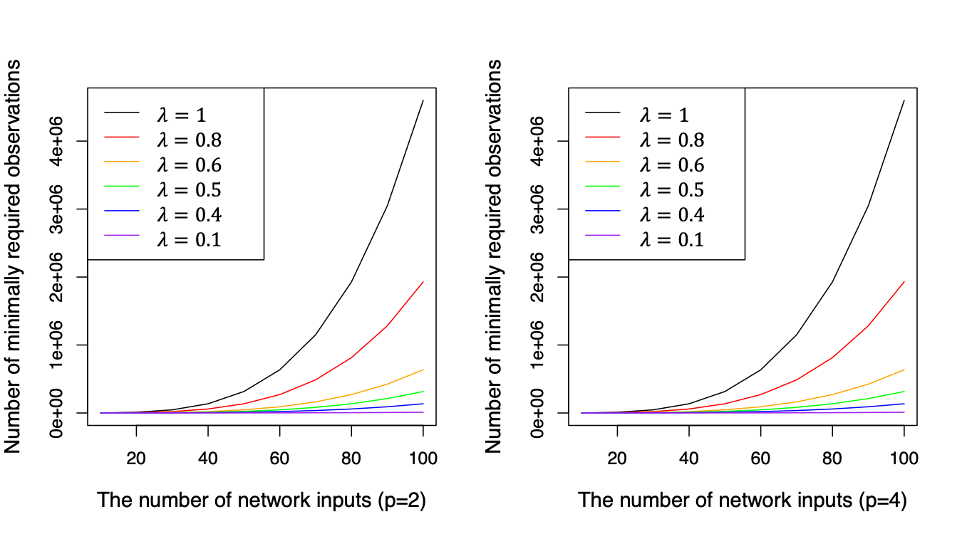
Figure 2: Network PCE ($\lambda<1$) requires fewer observations to model the network output than naïve PCE ($\lambda=1$) for a larger $p$ (the highest polynomial order used in both PCEs) and a smaller $\lambda$. $\lambda$, defined in eq. (22), represents the ratio of the largest number of variables used in any PCE for network PCE to the number of network inputs used in naïve PCE.

III-D Sparse network PCE (SN-PCE)

While the proposed network PCE already provides substantial parsimony over naïve PCE, it may still need to use many orthonormal polynomials to capture all the main effects and the major interaction effects of the network variables on the output variance. However, in practice, many of such effects are insignificant. Therefore, we propose SN-PCE, which imposes $l_{1}$-sparsity on the PCE coefficients to capture only significant pathways of uncertainty propagation in the network. Specifically, SN-PCE solves an equivalent problem of eq. (LABEL:eq:lasso) (with the difference lying only in the notations) instead of eq. (LABEL:eq:over_lin) in Steps 3 and 4 of Algorithm 2. The resulting parsimonious model can use even fewer observations than network PCE to estimate the PCE coefficients and, in turn, the Sobol indices. Also, because only significant effects appear in the model (with non-zero PCE coefficients), the model is easier to interpret than the other models.

III-E Theoretical result

Since naïve PCE is a direct application of standard PCE in eq. (1), the corresponding theoretical result (Theorem 1) directly follows from [14] by appropriately invoking Assumption 1 below. The result is still presented here mainly for comparison with the theoretical result on network PCE (Theorem 3).

Assumption 1 (adapted from [14]).

The random vector $\bm{x}\coloneqq(x_{1},\ldots,x_{n})^{T}:(\Omega,\mathcal{F})\rightarrow\left(\mathbb{A}^{n},\mathcal{B}^{n}\right)$

1. has a continuous joint probability density function $\mu(\bm{x})$ with a bounded or unbounded support $\mathbb{A}^{n}\subseteq\mathbb{R}^{n}$;

2. possesses absolute finite moments of all orders, that is, $\forall\mathbf{j}\coloneqq(j_{1},j_{2},\ldots,j_{n})\in\mathbb{N}_{0}^{n}$,

   $$\mathbb{E}\left(\left|\bm{x}^{\mathbf{j}}\right|\right):=\int_{\Omega}\left|\bm{x}^{\mathbf{j}}(w)\right|d\mathcal{P}(w)<\infty,$$

   where $\bm{x}^{\mathbf{j}}:=x_{1}^{j_{1}}\cdots x_{n}^{j_{n}}$; and

3. has a joint probability density function $\mu(\bm{x})$, which

   1. has a compact support, that is, there exists a compact subset $\mathbb{A}^{n}\subset\mathbb{R}^{n}$ such that $\mathcal{P}(\bm{x}\in\mathbb{A}^{n})=1$, or

   2. is exponentially integrable, that is, there exists a real number $\alpha>0$ such that

      $$\int_{\mathbb{A}^{n}}\exp\left(\alpha||\bm{x}||\right)\mu(\bm{x})\,d\bm{x}<\infty,$$

      where $||\cdot||:\mathbb{A}^{n}\rightarrow\mathbb{R}_{0}^{+}$ is an abitrary norm.

Theorem 1.

Suppose that for the network output $y\!\left(\bm{\xi}\right)\in\mathcal{L}^{2}\!\left(\Omega,\mathcal{F},\mathcal{P}\right)$, $\bm{\xi}=\bm{x}_{S(G)\cap V_{y}}$ fulfills Assumption 1. Then, $\hat{y}$ in eq. (10) converges to $y$ in probability as $P\to\infty$.

Proof.

This is a direct result of Theorem 11 in [14]. ∎

Theorem 1 imposes regularity conditions on the network inputs $\bm{\xi}$ and output $y$, but not on the other network variables. This black-box approach of naïve PCE still provides a convergent prediction of $y$ as $P\to\infty$. In practice, increasing $P$ requires increasing the number of observations. Thus, the finite-sample inefficiency of naïve PCE compared to network PCE (described in Sec. III-C) is critical when the sample size is limited.

Theoretical results on network PCE impose regularity conditions on all the network variables as the knowledge of network structure provides network PCE’s advantage over naïve PCE. Lemma 2 validates the recursive modeling of a network node using its direct predecessors (described in Steps 1–5 in Algorithm 2). Building on Lemma 2, Theorem 3 proves the convergence of network PCE output in eq. (18).

Lemma 2.

Suppose that $\bm{x}_{\bm{v}_{j}^{(l)}}$ is a function of $\mathscr{P}\!\left(\bm{x}_{\bm{v}_{j}^{(l)}}\right)$ for $l=1,\ldots,L-1$ and $j=1,\ldots,n^{(l)}$, and that for the network output $y$, $\bm{x}_{V_{y}}$ fulfills Assumption 1. Then,

1. $\hat{\psi}_{\bm{\alpha}_{ij}^{(l)}}^{(l)}\left(\bm{x}_{\bm{v}_{j}^{(l)}}\right)$ in eq. (14) converges to $\psi_{\bm{\alpha_{ij}}^{(l)}}^{(l)}\left(\bm{x}_{\bm{v}_{j}^{(l)}}\right)$ in eq. (13) in probability as $P_{ij}^{(l)}\to\infty$; and

2. $\hat{\psi}_{i}^{(l)}\left(\mathscr{P}^{l}\left(y\right)\right)=\prod_{j=1}^{n^{(l)}}\hat{\psi}_{\bm{\alpha}_{ij}^{(l)}}^{(l)}\left(\bm{x}_{\bm{v}_{j}^{(l)}}\right)$ in eq. (LABEL:eq:iter1) converges to $\psi^{(l)}_{i}\left(\mathscr{P}^{l}(y)\right)$ in eq. (13) in probability as $P_{ij}^{(l)}\to\infty$

for all $l=1,\ldots,L-1$ and all $\bm{\alpha}_{i}^{(l)}=\left(\bm{\alpha}_{i1}^{(l)},\ldots,\bm{\alpha}_{in^{(l)}}^{(l)}\right)$ satisfying $\sum_{j=1}^{n^{(l)}}\left|\bm{\alpha}_{ij}^{(l)}\right|\leq p^{(l)}$.

Proof.

Under the stated assumptions, $\psi_{\bm{\alpha_{ij}}^{(l)}}^{(l)}\left(\bm{x}_{\bm{v}_{j}^{(l)}}\right)$ in eq. (13) is a square-integrable function of $\mathscr{P}\!\left(\bm{x}_{\bm{v}_{j}^{(l)}}\right)$. The first statement follows from Theorem 11 in [14]. The second statement follows from the first statement by the continuous mapping theorem. ∎

Theorem 3.

Suppose that the assumptions in Lemma 2 hold for the network output $y\!\left(\bm{x}_{\bm{v}^{(1)}}\right)\in\mathcal{L}^{2}\!\left(\Omega,\mathcal{F},\mathcal{P}\right)$. Then, there exists an increasing function $\gamma^{(l)}\!:\mathbb{N}\mapsto\mathbb{N}$ such that if $p^{(l+1)}=\gamma^{(l)}\!\left(P^{(l)}\right)$ for $l=1,\ldots,L-1$, $\hat{y}^{(L)}$ in eq. (18) converges to $y$ in probability as $p^{(1)}\to\infty$, or equivalently, $P^{(1)}\to\infty$.

Proof.

The proof is provided in the article’s online supplementary document. ∎

The increasing function $\gamma^{(l)}$ in Theorem 3 prescribes how fast the highest polynomial order $p^{(l+1)}=\gamma^{(l)}\!\left(P^{(l)}\right)$ should grow in relation to the number of orthonormal polynomials, $P^{(l)}$, for $l=1,\ldots,L-1$ so that $\hat{y}^{(L)}$ in eq. (18) converges to $y$ in probability. Furthermore, to make the relation between $p^{(l+1)}$ and $p^{(l)}$ more explicit, using eqs. (20) and (21), let $d^{(1)}:=\left|D_{y}\right|$ and $d^{(l)}:=\left|\underset{1\leq j\leq n^{(l)}}{\bigcup}D_{j}^{(l-1)}\right|$, $l=2,\ldots,L$, denote the number of nodes represented by $\mathscr{P}\!\left(y\right)$ and $\mathscr{P}^{l}\!\left(y\right)$ in eq. (12), respectively. Because

$$P^{(l)}+1=\binom{d^{(l)}+p^{(l)}}{d^{(l)}},$$

for $l=1,\ldots,L$, Stirling’s approximation yields

$$p^{(l+1)}=\gamma^{(l)}\!\left(O\!\left(\left(p^{(l)}\right)^{d^{(l)}}\right)\right)$$

using the big O notation.

For example, if $\gamma^{(l)}$ is linear (or superlinear), then $p^{(l+1)}$ should grow as fast as (or faster than) $d^{(l)}$-th power of $p^{(l)}$, or equivalently, $\prod_{l^{\prime}=1}^{l}d^{(l^{\prime})}$-th power of $p^{(1)}$ for $l=1,\ldots,L-1$. Intuitively speaking, we should control the approximation errors for the upstream nodes in the network more tightly to ensure that the approximation errors for the downstream nodes (especially the output node) are arbitrarily small. We note that it is beyond the scope of this paper to establish more detailed characteristics of $\gamma^{(l)}$.

SN-PCE, which tends to use much smaller $P^{(l)},l=1,\ldots,L$, than network PCE, mitigates the need for rapidly increasing $p^{(l)},l=1,\ldots,L$, while maintaining a similar approximation accuracy.

IV Applications

For empirical evaluation of the proposed methodology, we conduct sensitivity analysis of two manufacturing processes (welding and injection molding) in [35]. We use the same modeling equations and notations therein (hence, some notation conflicts arise although their meanings are clear from the context). Note that the proposed methodology leverages the known directional relationships between inputs and the output (expressed as a DAG), not modeling equations, which are often unknown in practice.

We compare four methods, namely, random sampling [36], orthogonal array sampling [37], naïve PCE, and SN-PCE, for estimating the first-order and total Sobol indices. The estimation is replicated 50 times to calculate the sample mean and standard error of the estimated Sobol indices for each method.

As discussed in Sec. II-E, the Sobol indices measure the influence of each network input on the variance of the network output. Henceforth, we call some network inputs influential inputs if their first-order Sobol indices are $10^{-1}$ or larger; in other words, the influential inputs explain 10% or more of the output variance without considering their interactions with the other inputs.

We use a large sample for random and orthogonal array sampling, namely, 10,000 observations unless specified otherwise. We treat the sample mean from 50 replications using the orthogonal array sampling as the ground truth if the standard error is below 1% of the sample mean. Even with a large sample, such Monte Carlo sampling methods tend to have large standard errors for estimating small total Sobol indices [38, 36], as also observed in this study.

IV-A Welding process

Figure 3: This DAG represents the relationships among the variables in the welding process [35]; the weld volume $V$ depends on six welding parameters (weld zone dimensions: $e$, $g$, $h$, $l$, and $t$; weld length $L$), and the total energy $E$ depends on $V$ and additional parameters, $\rho$, $C_{p}$, $T_{i}$, $T_{f}$, and $H$.

The welding process has several process variables whose relationships are depicted in Fig. 3. The process output of interest is the total minimum theoretical energy required for the welding process, $E$. This energy depends on the weld volume $V$, specific gravity $\rho$, heat capacity $C_{p}$, initial temperature $T_{i}$, final temperature $T_{f}$, and latent heat $H$ as follows:

$$E=\rho V\left(C_{p}(T_{f}-T_{i})+H\right).$$

In turn, the weld volume $V$ depends on six welding parameters (weld zone dimensions: $e$, $g$, $h$, $l$, and $t$; weld length $L$) as follows:

$$V=L\left(0.75lh+gt+0.5(l-9)(t-e)\right).$$

The process inputs’ distributions are presented in Table I.

We first compare the four methods with respect to the mean squared errors of estimating the Sobol indices when using the same sample size. Fig. 4 shows that SN-PCE significantly outperforms random and orthogonal array sampling. Also, SN-PCE estimates the Sobol indices using a much smaller sample size than naïve PCE. In this example, we use the highest polynomial order of $3$ for both naïve PCE and SN-PCE; naïve PCE requires at least $364=\binom{11+3}{3}$ observations for $\dim\!\left(\bm{\xi}\right)=11$ and network PCE (i.e., SN-PCE without sparsity) requires at least $84=\binom{6+3}{3}$ observations because eq. (19) equals 6. SN-PCE could use even fewer observations because it identifies only $14$ orthonormal polynomials (4% of those used in naïve PCE) as necessary to approximate the network output of this particular process across all the 50 replications.

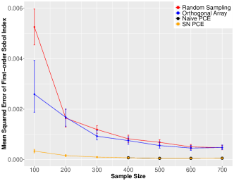
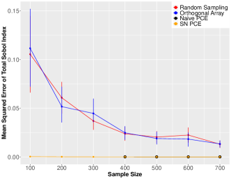
Figure 4: SN-PCE yields a smaller mean squared error of estimating the first-order Sobol indices (left) and the total Sobol indices (right) than the three other methods for the welding process. Also, SN-PCE requires much fewer observations than naïve PCE to estimate the Sobol indices.

Table I shows the sample means and standard errors of the estimated Sobol indiceses for the four methods, where naïve PCE and SN-PCE use 500 and 100 observations, respectively. Despite the vastly different sample sizes used for each method, the sample means are nearly identical across the methods (except for the non-influential inputs, which have total Sobol indices smaller than $10^{-1}$). This indicates the estimation bias is nearly zero for these methods. The standard errors are also very similar across the methods for the influential inputs, indicating that SN-PCE achieves a similar accuracy as the other methods with a much smaller sample size.

Fig. 5 presents a Pareto chart of the first-order Sobol indices estimated from SN-PCE. Along with Table II, the chart confirms that the weld zone dimensions ($h,g,t,e,l)$ are the most influential inputs for the variance of the process output $E$. Also, the cumulative sum of the first-order Sobol indices approaches 100% in the chart, implying that the interactions between the inputs do not have significant effects on the variance of $E$. It echoes the finding from Table II that the first-order Sobol indices are approximately equal to the total Sobol indices across all the influential inputs.

TABLE I: Sample means and standard errors (rounded to two decimal places) of the estimated first-order and total Sobol indices based on 50 replications for the welding process. The inputs in the first column are sorted in descending order of the first-order Sobol indices estimated from the Monte Carlo method. For each replication, $\dagger$random sampling, $\ddagger$orthogonal array sampling, $\dagger\dagger$Naïve PCE, and $\ddagger\ddagger$SN-PCE use 10,000, 10,000, 500, and 100 observations, respectively. For the influential inputs, SN-PCE attains similar standard errors as the other methods despite using the smallest sample size.

Input Distribution $\text{Random Sampling}^{\dagger}$ $\text{Orthogonal Array}^{\ddagger}$ $\text{Na\"{\i}ve PCE}^{\dagger\dagger}$ $\text{SN-PCE}^{\ddagger\ddagger}$ First-order Total First-order Total First-order Total First-order Total $h$ $N(2.6,0.5)$ $2.76\times 10^{-1}$ $2.85\times 10^{-1}$ $2.78\times 10^{-1}$ $2.81\times 10^{-1}$ $2.78\times 10^{-1}$ $2.80\times 10^{-1}$ $2.80\times 10^{-1}$ $2.81\times 10^{-1}$ $\pm 0.02\times 10^{-1}$ $\pm 0.04\times 10^{-1}$ $\pm 0.01\times 10^{-1}$ $\pm 0.03\times 10^{-1}$ $\pm 0.01\times 10^{-1}$ $\pm 0.01\times 10^{-1}$ $\pm 0.02\times 10^{-1}$ $\pm 0.02\times 10^{-1}$ $g$ $N(2,0.1)$ $2.31\times 10^{-1}$ $2.30\times 10^{-1}$ $2.34\times 10^{-1}$ $2.32\times 10^{-1}$ $2.32\times 10^{-1}$ $2.33\times 10^{-1}$ $2.34\times 10^{-1}$ $2.35\times 10^{-1}$ $\pm 0.01\times 10^{-1}$ $\pm 0.03\times 10^{-1}$ $\pm 0.01\times 10^{-1}$ $\pm 0.03\times 10^{-1}$ $\pm 0.01\times 10^{-1}$ $\pm 0.01\times 10^{-1}$ $\pm 0.02\times 10^{-1}$ $\pm 0.02\times 10^{-1}$ $t$ $N(15,0.6)$ $2.29\times 10^{-1}$ $2.24\times 10^{-1}$ $2.27\times 10^{-1}$ $2.32\times 10^{-1}$ $2.29\times 10^{-1}$ $2.29\times 10^{-1}$ $2.25\times 10^{-1}$ $2.26\times 10^{-1}$ $\pm 0.01\times 10^{-1}$ $\pm 0.03\times 10^{-1}$ $\pm 0.01\times 10^{-1}$ $\pm 0.04\times 10^{-1}$ $\pm 0.01\times 10^{-1}$ $\pm 0.01\times 10^{-1}$ $\pm 0.02\times 10^{-1}$ $\pm 0.02\times 10^{-1}$ $e$ $N(11,1)$ $1.46\times 10^{-1}$ $1.48\times 10^{-1}$ $1.46\times 10^{-1}$ $1.50\times 10^{-1}$ $1.45\times 10^{-1}$ $1.47\times 10^{-1}$ $1.46\times 10^{-1}$ $1.48\times 10^{-1}$ $\pm 0.01\times 10^{-1}$ $\pm 0.04\times 10^{-1}$ $\pm 0.01\times 10^{-1}$ $\pm 0.04\times 10^{-1}$ $\pm 0.01\times 10^{-1}$ $\pm 0.01\times 10^{-1}$ $\pm 0.01\times 10^{-1}$ $\pm 0.01\times 10^{-1}$ $l$ $N(8.5,0.5)$ $1.07\times 10^{-1}$ $1.08\times 10^{-1}$ $1.08\times 10^{-1}$ $1.12\times 10^{-1}$ $1.07\times 10^{-1}$ $1.12\times 10^{-1}$ $1.08\times 10^{-1}$ $1.12\times 10^{-1}$ $\pm 0.01\times 10^{-1}$ $\pm 0.04\times 10^{-1}$ $\pm 0.01\times 10^{-1}$ $\pm 0.04\times 10^{-1}$ $\pm 0.00\times 10^{-1}$ $\pm 0.00\times 10^{-1}$ $\pm 0.01\times 10^{-1}$ $\pm 0.01\times 10^{-1}$ $L$ $N(500,10)$ $1.96\times 10^{-3}$ $4.45\times 10^{-4}$ $1.95\times 10^{-3}$ $2.57\times 10^{-3}$ $1.96\times 10^{-3}$ $2.00\times 10^{-3}$ $1.94\times 10^{-3}$ $1.95\times 10^{-3}$ $\pm 0.01\times 10^{-3}$ $\pm 43.4\times 10^{-4}$ $\pm 0.01\times 10^{-3}$ $\pm 4.25\times 10^{-3}$ $\pm 0.01\times 10^{-3}$ $\pm 0.01\times 10^{-3}$ $\pm 0.03\times 10^{-3}$ $\pm 0.03\times 10^{-3}$ $C_{\rho}$ $N(500,5)$ $9.67\times 10^{-4}$ $-9.76\times 10^{-4}$ $9.66\times 10^{-4}$ $4.94\times 10^{-6}$ $9.69\times 10^{-4}$ $9.89\times 10^{-4}$ $9.77\times 10^{-4}$ $9.77\times 10^{-4}$ $\pm 0.07\times 10^{-4}$ $\pm 43.02\times 10^{-4}$ $\pm 0.05\times 10^{-4}$ $\pm 0.04\times 10^{-2}$ $\pm 0.05\times 10^{-4}$ $\pm 0.05\times 10^{-4}$ $\pm 0.15\times 10^{-4}$ $\pm 0.15\times 10^{-4}$ $T_{f}$ $N(1628,10)$ $2.75\times 10^{-4}$ $-1.64\times 10^{-3}$ $2.76\times 10^{-4}$ $1.50\times 10^{-6}$ $2.75\times 10^{-4}$ $2.81\times 10^{-4}$ $7.55\times 10^{-5}$ $7.55\times 10^{-5}$ $\pm 0.02\times 10^{-4}$ $\pm 4.35\times 10^{-3}$ $\pm 0.05\times 10^{-4}$ $\pm 4.25\times 10^{-3}$ $\pm 0.01\times 10^{-4}$ $\pm 0.01\times 10^{-4}$ $\pm 1.02\times 10^{-5}$ $\pm 1.02\times 10^{-5}$ $T_{i}$ $N(303,0.3)$ $8.32\times 10^{-6}$ $-1.74\times 10^{-3}$ $8.23\times 10^{-6}$ $2.76\times 10^{-4}$ $8.28\times 10^{-6}$ $8.45\times 10^{-6}$ 0 0 $\pm 0.04\times 10^{-6}$ $\pm 0.04\times 10^{-3}$ $\pm 0.05\times 10^{-6}$ $\pm 4.25\times 10^{-3}$ $\pm 0.04\times 10^{-6}$ $\pm 0.04\times 10^{-6}$ $\rho$ $N(8238,10)$ $7.23\times 10^{-6}$ $-1.78\times 10^{-3}$ $7.20\times 10^{-6}$ $4.06\times 10^{-8}$ $7.16\times 10^{-6}$ $7.30\times 10^{-6}$ 0 0 $\pm 0.05\times 10^{-6}$ $\pm 4.31\times 10^{-3}$ $\pm 4.06\times 10^{-8}$ $\pm 4.25\times 10^{-3}$ $\pm 0.03\times 10^{-6}$ $\pm 0.03\times 10^{-6}$ $H$ $N(2270,3)$ $3.32\times 10^{-10}$ $-1.77\times 10^{-3}$ $3.30\times 10^{-10}$ $1.94\times 10^{-12}$ $3.31\times 10^{-10}$ $3.41\times 10^{-10}$ 0 0 $\pm 0.02\times 10^{-10}$ $\pm 4.32\times 10^{-3}$ $\pm 0.02\times 10^{-10}$ $\pm 4.25\times 10^{-3}$ $\pm 4.25\times 10^{-3}$ $\pm 0.02\times 10^{-10}$

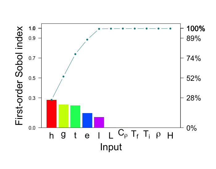
Figure 5: Pareto chart of the first-order Sobol indices estimated using SN-PCE for the welding process. Higher bar indicates that the input has a more influence (excluding interactions with other inputs) on the variance of the process output $E$.

IV-B Injection molding process

The injection molding process has more intricate relationships between process variables than the welding process, as depicted in Fig. 6. The process output of interest is the energy consumed in resetting the process, $E_{reset}$. This energy depends on the melting energy $E_{melt}$, the injection energy $E_{inj}$, and the cooling energy $E_{cool}$ as follows: $E_{reset}=0.25\left(E_{melt}+E_{inj}+E_{cool}\right)$. Here, $E_{melt}={P_{melt}\times V_{shot}}/{Q}$, where

$$P_{melt} =\frac{1}{2}\left(\rho\times Q\times C_{p}\times\left(T_{inj}-T_{pol}\right)+\rho\times Q\times H_{f}\right),$$

$$V_{shot} =V_{part}\times\left(1+\frac{\epsilon}{100}+\frac{\Delta}{100}\right).$$

Here, $\rho$ (specific gravity), $C_{p}$ (heat capacity), $T_{pol}$ (initial polymer temperature), $\epsilon$ (shrinkage parameter), and $T_{inj}$ (injection temperature) are the network inputs. $Q$ (flow rate), $H_{f}$ (polymer heat of fusion), $V_{part}$ (volume of mold), and $\Delta$ (buffer) are constant parameters. On the other hand, $E_{inj}=P_{inj}\times V_{part}$ and

$$E_{cool} =\frac{\rho\times V_{part}\times\left(C_{p}\times\left(T_{inj}-T_{ej}\right)\right)}{COP},$$

where $P_{inj}$ (injection pressure), $T_{ej}$ (ejection temperature), and $T_{inj}$ (injection temperature) are the network inputs. $COP$ (coefficient of performance of the cooling equipment) is a constant parameter. The network inputs’ distributions are presented in Table II.

Figure 6: This DAG represents the relationships among the variables in the injection molding process [35]; the yellow shaded nodes $E_{melt}$, $E_{cool}$, and $E_{inj}$ are the energies consumed in three subprocesses that depend on different blue shaded network inputs. The network output $E_{reset}$ depends on $E_{melt}$, $E_{cool}$, and $E_{inj}$.

To adequately model the more intricate network structure of the injection molding process, we use the highest polynomial order of $4$ for both naïve PCE and SN-PCE, compared to $3$ used for the welding process; naïve PCE requires at least $330=\binom{7+4}{4}$ observations for $\dim\!\left(\bm{\xi}\right)=7$ and network PCE (i.e., SN-PCE without sparsity) requires at least $126=\binom{5+4}{4}$ observations because eq. (19) equals 5. Thus, we use 500 and 200 observations for naïve PCE and SN-PCE, respectively, compared to 500 and 100 used for the welding process. Yet, again, SN-PCE could use even fewer observations because it identifies only $9$ orthonormal polynomials (3% of those used in naïve PCE) as necessary to approximate the network output of this particular process across all 50 replications.

TABLE II: Sample means and standard errors (rounded to two decimal places) of the estimated first-order Sobol indices based on 50 replications for the injection molding process. For each replication, $\ddagger\ddagger$SN-PCE uses 200 observations. All the other setups are the same as in Table I.

Input Distribution $\text{Random Sampling}^{\dagger}$ $\text{Orthogonal Array}^{\ddagger}$ $\text{Naive PCE}^{\dagger\dagger}$ $\text{SN-PCE}^{\ddagger\ddagger}$ $T_{inj}$ $N(210,3)$ $4.76\times 10^{-1}$ $4.75\times 10^{-1}$ $4.77\times 10^{-1}$ $4.78\times 10^{-1}$ $\pm 0.02\times 10^{-1}$ $\pm 0.02\times 10^{-1}$ $\pm 0.01\times 10^{-1}$ $\pm 0.02\times 10^{-1}$ $T_{ej}$ $N(35,3)$ $2.61\times 10^{-1}$ $2.61\times 10^{-1}$ $2.62\times 10^{-1}$ $2.61\times 10^{-1}$ $\pm 0.01\times 10^{-1}$ $\pm 0.01\times 10^{-1}$ $\pm 0.01\times 10^{-1}$ $\pm 0.01\times 10^{-1}$ $\rho$ $U(950,990)$ $2.27\times 10^{-1}$ $2.27\times 10^{-1}$ $2.26\times 10^{-1}$ $2.26\times 10^{-1}$ $\pm 0.01\times 10^{-1}$ $\pm 0.01\times 10^{-1}$ $\pm 0.00\times 10^{-1}$ $\pm 0.01\times 10^{-1}$ $T_{pol}$ $N(40,3)$ $3.22\times 10^{-2}$ $3.22\times 10^{-2}$ $3.21\times 10^{-2}$ $3.20\times 10^{-2}$ $\pm 0.02\times 10^{-2}$ $\pm 0.02\times 10^{-2}$ $\pm 0.02\times 10^{-2}$ $\pm 0.02\times 10^{-2}$ $C_{\rho}$ $U(2250,2260)$ $2.61\times 10^{-3}$ $2.62\times 10^{-3}$ $2.61\times 10^{-3}$ $2.61\times 10^{-3}$ $\pm 0.01\times 10^{-3}$ $\pm 0.01\times 10^{-3}$ $\pm 0.01\times 10^{-3}$ $\pm 0.01\times 10^{-3}$ $\epsilon$ $U(0.018,0.021)$ $7.76\times 10^{-9}$ $7.74\times 10^{-9}$ $7.76\times 10^{-9}$ $0$ $\pm 0.04\times 10^{-9}$ $\pm 0.04\times 10^{-9}$ $\pm 0.03\times 10^{-9}$ $P_{inj}$ $N(90,4)$ $4.75\times 10^{-14}$ $4.73\times 10^{-14}$ $4.77\times 10^{-14}$ $0$ $\pm 0.02\times 10^{-14}$ $\pm 0.02\times 10^{-14}$ $\pm 0.02\times 10^{-14}$

Like the welding process, the injection molding process turns out to have the first-order Sobol indices approximately equal to the total Sobol indices for the influential inputs. Thus, we only report the first-order Sobol indices in Table II. Again, SN-PCE attains similar standard errors as the other methods for the influential inputs despite using fewer observations. Fig. 7 shows that $T_{inj}$ determines nearly 50% of the variance of network output $E_{reset}$. $T_{ej}$ and $\rho$ have comparable effects ($26\%$ and $23\%$, respectively), while other inputs, $T_{pol}$, $C_{\rho}$, $\epsilon$, and $P_{inj}$, barely influence the variance of $E_{reset}$.

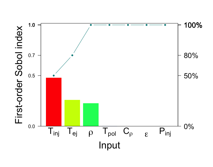
Figure 7: Pareto chart of the first-order Sobol indices estimated using SN-PCE for the injection molding process. Higher bar indicates that the input has a more influence (excluding interactions with other inputs) on the variance of process output $E_{reset}$.

V Conclusion

This paper proposes SN-PCE to model uncertainty propagation in a broad class of processes represented as DAGs. A DAG encodes the dependencies between the variables in a process, including the process output (sink node in the DAG) and inputs (source nodes in the DAG). SN-PCE effectively captures how the inputs influence the output variance. Theoretically, it is shown that network PCE (equivalent to SN-PCE without sparsity) is valid in the sense that its prediction of the output converges in probability to the true output under reasonable assumptions. Empirically, SN-PCE is shown to accurately estimate the Sobol indices of the output with respect to the inputs for two manufacturing processes and a flooding process. SN-PCE uses substantially fewer observations than the black-box approaches (Monte Carlo sampling methods and naïve PCE) to accurately identify the influential inputs, showing promise for efficient sensitivity analysis in process automation.

Future research may investigate extension of the proposed model to even more general networks. One direction could be to relax the assumption of mutual independence of the network inputs. While their dependencies would complicate the estimation and interpretation of the sensitivity indices, the indices proposed in [29] might help decode how the dependent network inputs influence the output. Another research direction would be to allow cycles (or, feedback loops) in the network, thereby, extending this work beyond directed acyclic networks. Lastly, while domain experts can often identify DAGs of their systems, machine learning can more efficiently identify complex DAGs from data under the causal Markov and causal faithfulness conditions [39, 40]. Future research may investigate the best way to combine network identification methods with the proposed method in this paper.

Zhanlin Liu received the B.S. degree in Statistics from University of Iowa, Iowa City, IA, USA, in 2014, and the M.S. degree in Statistics from the University of Washington, Seattle, WA, USA, in 2016. He is currently working toward the Ph.D. degree in Industrial $\&$ Systems Engineering at the University of Washington, Seattle, WA, USA. His current research interests include uncertainty quantification, reliability analysis, and statistical modeling.

Ashis G. Banerjee (S’08-M’09) received the B.Tech. degree in Manufacturing Science and Engineering from the Indian Institute of Technology Kharagpur, Kharagpur, India, in 2004, the M.S. degree in Mechanical Engineering from the University of Maryland (UMD), College Park, MD, USA, in 2006, and the Ph.D. degree in Mechanical Engineering from UMD in 2009. He is currently an Assistant Professor of Industrial & Systems Engineering and Mechanical Engineering at the University of Washington, Seattle, WA, USA. Prior to this appointment, he was a Research Scientist at GE Global Research, Niskayuna, NY, USA. Previously, he was a Research Scientist and Postdoctoral Associate in the Computer Science and Artificial Intelligence Laboratory at Massachusetts Institute of Technology, Cambridge, MA, USA. His research interests include digital manufacturing, predictive and prescriptive analytics, and autonomous robotics.

Youngjun Choe received the B.Sc. degrees in Physics and Management Science from KAIST, Korea in 2010, and both M.A. in Statistics and Ph.D. in Industrial & Operations Engineering from the University of Michigan, Ann Arbor, MI, USA in 2016. He is currently an Assistant Professor of Industrial & Systems Engineering at the University of Washington, Seattle, WA, USA. His research centers around developing statistical methods to infer on extreme events.

References

• [1] D. Djurdjanovic and J. Ni, “Stream-of-variation (SoV)-based measurement scheme analysis in multistation machining systems,” IEEE Transactions on Automation Science and Engineering, vol. 3, no. 4, pp. 407–422, 2006.
• [2] J. A. Marvel, “Performance metrics of speed and separation monitoring in shared workspaces,” IEEE Transactions on Automation Science and Engineering, vol. 10, no. 2, pp. 405–414, 2013.
• [3] A. Avdonin, S. Jaensch, C. F. Silva, M. Češnovar, and W. Polifke, “Uncertainty quantification and sensitivity analysis of thermoacoustic stability with non-intrusive polynomial chaos expansion,” Combustion and Flame, vol. 189, pp. 300–310, 2018.
• [4] P. C. Chen, V. Malbasa, Y. Dong, and M. Kezunovic, “Sensitivity analysis of voltage sag based fault location with distributed generation,” IEEE Transactions on Smart Grid, vol. 6, no. 4, pp. 2098–2106, 2015.
• [5] F. Ni, M. Nijhuis, P. H. Nguyen, and J. F. Cobben, “Variance-based global sensitivity analysis for power systems,” IEEE Transactions on Power Systems, vol. 33, no. 2, pp. 1670–1682, 2018.
• [6] S. Li, K. Deng, and M. Zhou, “Sensitivity analysis for building energy simulation model calibration via algorithmic differentiation,” IEEE Transactions on Automation Science and Engineering, vol. 14, no. 2, pp. 905–914, 2017.
• [7] W. Huang and Z. Kong, “Process capability sensitivity analysis for design evaluation of multistage assembly processes,” IEEE Transactions on Automation Science and Engineering, vol. 7, no. 4, pp. 736–745, 2010.
• [8] I. M. Sobol, “Sensitivity estimates for nonlinear mathematical models,” Mathematical Modelling and Computational Experiments, vol. 1, no. 4, pp. 407–414, 1993.
• [9] B. Sudret, “Meta-models for structural reliability and uncertainty quantification,” arXiv preprint arXiv:1203.2062, 2012.
• [10] R. J. Prill, P. A. Iglesias, and A. Levchenko, “Dynamic properties of network motifs contribute to biological network organization,” PLoS Biology, vol. 3, no. 11, pp. 1881–1892, 2005.
• [11] D. Mogale, S. K. Kumar, and M. K. Tiwari, “Two stage Indian food grain supply chain network transportation-allocation model,” IFAC-PapersOnLine, vol. 49, no. 12, pp. 1767–1772, 2016.
• [12] K. He, M. Jia, and Q. Xu, “Optimal sensor deployment for manufacturing process monitoring based on quantitative cause-effect graph,” IEEE Transactions on Automation Science and Engineering, vol. 13, no. 2, pp. 963–975, 2016.
• [13] P. Agrawal and S. Rao, “Energy-aware scheduling of distributed systems,” IEEE Transactions on Automation Science and Engineering, vol. 11, no. 4, pp. 1163–1175, 2014.
• [14] S. Rahman, “A polynomial chaos expansion in dependent random variables,” Journal of Mathematical Analysis and Applications, vol. 464, no. 1, pp. 749–775, 2018.
• [15] R. H. Cameron and W. T. Martin, “The orthogonal development of non-linear functionals in series of Fourier-Hermite functionals,” Annals of Mathematics, vol. 48, no. 2, pp. 385–392, 1947.
• [16] M. P. Pettersson, G. Iaccarino, and J. Nordström, Polynomial chaos methods for hyperbolic partial differential equations.   Springer, 2015.
• [17] G. Blatman and B. Sudret, “Efficient computation of global sensitivity indices using sparse polynomial chaos expansions,” Reliability Engineering & System Safety, vol. 95, no. 11, pp. 1216–1229, 2010.
• [18] ——, “Adaptive sparse polynomial chaos expansion based on least angle regression,” Journal of Computational Physics, vol. 230, no. 6, pp. 2345–2367, 2011.
• [19] J. D. Jakeman, M. S. Eldred, and K. Sargsyan, “Enhancing $\ell$1-minimization estimates of polynomial chaos expansions using basis selection,” Journal of Computational Physics, vol. 289, pp. 18–34, 2015.
• [20] J. Peng, J. Hampton, and A. Doostan, “On polynomial chaos expansion via gradient-enhanced $\ell$1-minimization,” Journal of Computational Physics, vol. 310, pp. 440–458, 2016.
• [21] Q. Shao, A. Younes, M. Fahs, and T. A. Mara, “Bayesian sparse polynomial chaos expansion for global sensitivity analysis,” Computer Methods in Applied Mechanics and Engineering, vol. 318, pp. 474–496, 2017.
• [22] K. Cheng and Z. Lu, “Sparse polynomial chaos expansion based on d-morph regression,” Applied Mathematics and Computation, vol. 323, pp. 17–30, 2018.
• [23] N. Wiener, “The homogeneous chaos,” American Journal of Mathematics, vol. 60, no. 4, pp. 897–936, 1938.
• [24] D. Xiu and G. E. Karniadakis, “The Wiener–Askey polynomial chaos for stochastic differential equations,” SIAM Journal on Scientific Computing, vol. 24, no. 2, pp. 619–644, 2002.
• [25] X. Wan and G. E. Karniadakis, “Multi-element generalized polynomial chaos for arbitrary probability measures,” SIAM Journal on Scientific Computing, vol. 28, no. 3, pp. 901–928, 2006.
• [26] S. Oladyshkin and W. Nowak, “Data-driven uncertainty quantification using the arbitrary polynomial chaos expansion,” Reliability Engineering & System Safety, vol. 106, pp. 179–190, 2012.
• [27] J. A. Witteveen, S. Sarkar, and H. Bijl, “Modeling physical uncertainties in dynamic stall induced fluid–structure interaction of turbine blades using arbitrary polynomial chaos,” Computers & Structures, vol. 85, no. 11, pp. 866–878, 2007.
• [28] M. Navarro, J. Witteveen, and J. Blom, “Polynomial chaos expansion for general multivariate distributions with correlated variables,” arXiv preprint arXiv:1406.5483, 2014.
• [29] Z. Liu and Y. Choe, “Data-driven sensitivity indices for models with dependent inputs using the polynomial chaos expansion,” arXiv preprint arXiv:1803.10978, 2018.
• [30] G. Chastaing, F. Gamboa, and C. Prieur, “Generalized Hoeffding-Sobol decomposition for dependent variables-application to sensitivity analysis,” Electronic Journal of Statistics, vol. 6, pp. 2420–2448, 2012.
• [31] T. Crestaux, O. Le Maître, and J. M. Martinez, “Polynomial chaos expansion for sensitivity analysis,” Reliability Engineering & System Safety, vol. 94, no. 7, pp. 1161–1172, 2009.
• [32] T. Homma and A. Saltelli, “Importance measures in global sensitivity analysis of nonlinear models,” Reliability Engineering & System Safety, vol. 52, no. 1, pp. 1–17, 1996.
• [33] B. Sudret, “Global sensitivity analysis using polynomial chaos expansions,” Reliability Engineering & System Safety, vol. 93, no. 7, pp. 964–979, 2008.
• [34] C. Carstens, “Motifs in directed acyclic networks,” in 2013 International Conference on Signal-Image Technology & Internet-Based Systems, 2013, pp. 605–611.
• [35] S. Nannapaneni and S. Mahadevan, “Uncertainty quantification in performance evaluation of manufacturing processes,” in 2014 IEEE International Conference on Big Data, 2014, pp. 996–1005.
• [36] A. B. Owen, “Better estimation of small Sobol’ sensitivity indices,” ACM Transactions on Modeling and Computer Simulation, vol. 23, no. 2, pp. 11–17, 2013.
• [37] J.-Y. Tissot and C. Prieur, “A randomized orthogonal array-based procedure for the estimation of first-and second-order sobol’indices,” Journal of Statistical Computation and Simulation, vol. 85, no. 7, pp. 1358–1381, 2015.
• [38] E. Myshetskaya, “Monte Carlo estimators for small sensitivity indices,” Monte Carlo Methods and Applications mcma, vol. 13, no. 5-6, pp. 455–465, 2008.
• [39] S. Meganck, P. Leray, and B. Manderick, “Learning causal Bayesian networks from observations and experiments: A decision theoretic approach,” in International Conference on Modeling Decisions for Artificial Intelligence.   Springer, 2006, pp. 58–69.
• [40] S. Huang, J. Li, J. Ye, A. Fleisher, K. Chen, T. Wu, E. Reiman, A. D. N. Initiative et al., “A sparse structure learning algorithm for Gaussian Bayesian network identification from high-dimensional data,” IEEE Transactions on Pattern Analysis and Machine Intelligence, vol. 35, no. 6, pp. 1328–1342, 2013.