Affinity-dependent bound on the spectrum of stochastic matrices

Abstract

Affinity has proven to be a useful tool for quantifying the non-equilibrium character of time continuous Markov processes since it serves as a measure for the breaking of time reversal symmetry. It has recently been conjectured that the number of coherent oscillations, which is given by the ratio of imaginary and real part of the first non-trivial eigenvalue of the corresponding master matrix, is constrained by the maximum cycle affinity present in the network. In this paper, we conjecture a bound on the whole spectrum of these master matrices that constrains all eigenvalues in a fashion similar to the well known Perron-Frobenius theorem that is valid for any stochastic matrix. As in other studies that are based on affinity-dependent bounds, the limiting process that saturates the bound is given by the asymmetric random walk. For unicyclic networks, we prove that it is not possible to violate the bound by small perturbation of the asymmetric random walk and provide numerical evidence for its validity in randomly generated networks. The results are extended to multicyclic networks, backed up by numerical evidence provided by networks with randomly constructed topology and transition rates.

1 Introduction

Real valued matrices with positive entries (with exception of the diagonal) can be encountered in many different fields of mathematics and physics. They show up in many forms and under different names throughout the literature. In graph theory they appear as the Laplacian matrix of (weighted) graphs [1], the time evolution of Markov chains is governed by a transition matrix that falls under this category, and most importantly for the scope of this article, the time evolution of a continuous time jump process is generated by a matrix of this type. Efforts to understand the structure of the spectrum of such matrices can ultimately result in insights into the studied system.

While many well known results like the Perron-Frobenius theorem or Gershgorin disks are quite general [2, 3, 4], in a physical context bounds on the spectrum that may be less general but depend on physically meaningful quantities are more desirable since they could be used to infer otherwise hidden properties of the system. In particular, for non-equilibrium systems coupled to thermal or chemical reservoirs such a strategy is called thermodynamic inference [5]. A recent, prominent example for such a relation is the thermodynamic uncertainty relation, which provides a lower bound to the rate of entropy production based on the observable precision of thermodynamic currents [6, 7, 8, 9]

Recent efforts to understand relations between the entropy production associated with maintaining biochemical oscillations [10, 11, 12] have sparked interest in fundamental connections between the non-equilibrium character of such reactions and the properties of the observed oscillations. It was conjectured that the affinity of the chemical network can be used to find a bound to the number of coherent oscillations shown by the dominant contribution to the corresponding relaxation process [13].

This finding begs the question, whether the dominant eigenvalue of the generator that governs the long time behavior is the only one for which affinity-dependent bounds apply or whether there are global bounds valid for all eigenvalues, i.e., for all timescales of the relaxation process. In this paper we argue that indeed the later is the case and there exist such a bound for the whole spectrum of the master equation.

This study is concerned with time continuous Markov processes on a discrete set of $N$ states. The state of the system jumps with rates $w_{ij}\geq 0$ from state $i$ to state $j$. Consequently, the probability $p_{i}(t)$ to occupy a certain state $i$ at time $t$ evolves according to the master equation

$$\partial_{t}p_{i}(t)=\sum_{j}M_{i,j}p_{j}(t)$$ (1)

with the generator $M_{i,j}$ that is of the form

$$M_{i,j}=w_{ji}-\delta_{i,j}r_{i}\,,$$ (2)

where the exit rate $r_{i}$ is the sum of all rates of jumps away from state $i$,i.e., $r_{i}=\sum_{j}w_{ij}$.

An important subclass of such networks that will be used as paradigmatic examples are unicyclic networks where the states are arranged in a cyclical fashion and only jumps between next neighbors are allowed. The generator then takes the form

$$M_{i,j}=w_{i+}\delta_{i,j+1}+w_{i-}\delta_{i,j-1}-(w_{i+}+w_{i-})\delta_{i,j}\,,$$ (3)

where we assume circular boundary conditions in the indices, i.e., we identify $N+1\hat{=}1$.

The objective of this article is to motivate and conjecture a bound that interpolates between the generic case covered by the Perron-Frobenius theorem and the special case of thermal equilibrium, where detailed balance holds.

2 Conjecture

An asymmetric random walk on a cycle of states is uniquely defined by the forward rate $w_{+}$, the backward rate $w_{-}$, and the number of states $N$. It can alternatively be defined using the exit rate $w_{0}=w_{+}+w_{-}$, the affinity $\mathcal{A}=N\ln(w_{+}/w_{-})$, and $N$. The corresponding generator reads

$$\mathbf{M}_{i,j}^{(0)}=w_{+}\delta_{i,j+1}+w_{-}\delta_{i,j-1}-(w_{+}+w_{-})\delta_{i,j}$$ (4)

with the rates

$$w_{+}=w_{0}\frac{e^{\mathcal{A}/(2N)}}{2\cosh(\mathcal{A}/(2N))}\quad\mathrm{and}\quad w_{-}=w_{0}\frac{e^{-\mathcal{A}/(2N)}}{2\cosh(\mathcal{A}/(2N))}\,.$$ (5)

It is a special case of a unicyclic system with $w_{i+}$ and $w_{i-}$ in equation (3) chosen uniformly for each link. This matrix is circulant and as such it can be diagonalized analytically leading to the eigenvectors

$$\ket{\nu^{0}_{n}}=\frac{1}{\sqrt{N}}\sum_{k=0}^{N-1}\exp(-2\pi\mathrm{i}nk/N)\ket{k}\,,$$ (6)

with the corresponding eigenvalues

$$\lambda_{n}=w_{0}\left[-1+\cos(2\pi n/N)+\mathrm{i}\tanh(\mathcal{A}/2N)\sin(2\pi n/N)\right]\,.$$ (7)

They lie on an ellipse on the complex plane. We conjecture that the eigenvalues of the generators of all unicyclic processes that have the same affinity, defined as $\mathcal{A}=\sum_{i}\ln(w_{i+}/w_{i-})$, the same maximum exit rate $w_{0}=\max_{i}(w_{i+}+w_{i-})$, and the same number of states, lie within the ellipse defined by the corresponding asymmetric random walk, as it is illustrated in figure 1. For multicyclic networks, we conjecture that the eigenvalues lie within the ellipse corresponding to the cycle $\mathcal{C}$ present in the network that maximizes the ratio $\mathcal{A}_{\mathcal{C}}/N_{\mathcal{C}}$, where $\mathcal{A}_{\mathcal{C}}$ and $N_{\mathcal{C}}$ denote the affinity and the number of states contained in cycle $\mathcal{C}$, respectively.

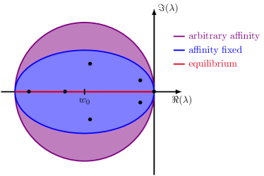
Figure 1: Scheme of regions in the complex plane within which the eigenvalues of a master matrix must lie. For generic master generators the Perron-Frobenius theorem restricts the eigenvalues to a circle on the negative half plane. If the system is in thermal equilibrium, in addition, all eigenvalues must be real. We conjecture an elliptical bound that depends on the maximum cycle affinity per state.

3 Motivation

Having stated the conjecture, we provide some rationale as to why this should be the case. If the system is in equilibrium, the transition rates have to satisfy detailed balance relations that connect the transition rates to the free energy $\mathcal{F}_{i}$ associated with the states according to [5]

$$\frac{w_{ij}}{w_{ji}}=\exp\left(\mathcal{F}_{j}-\mathcal{F}_{i}\right)\,.$$ (8)

A suitable set of free energies can be found if and only if the cycle affinity

$$\mathcal{A}_{\mathcal{C}}=\sum_{i\rightarrow j\in\mathcal{C}}\ln\frac{w_{ij}}{w_{ji}}\,$$ (9)

of all cycles in the network vanishes. As a consequence of the detailed balance relation, the generator satisfies the symmetry relation

$$\exp(\mathcal{F}_{j}/2)M_{j,i}\exp(-\mathcal{F}_{i}/2)=\exp(\mathcal{F}_{i}/2)M_{i,j}\exp(-\mathcal{F}_{j}/2)$$ (10)

and is thus similar to a symmetric matrix which means that its spectrum is real. This result agrees with our conjecture when taking the limit $\mathcal{A}\rightarrow 0$ in which case the ellipse degenerates to a line on the real axis.

For arbitrary affinities the Perron-Frobenius theorem guarantees that no eigenvalue of the generator lies outside the circle centered at $-w_{0}$ on the complex plane that touches the imaginary axis. This bound corresponds to our conjecture in the limit $\mathcal{A}/N\rightarrow\infty$.

An early indication that there is a connection between the distance from equilibrium and the spectrum can be found in works of Dimitriev and Dynkin on refinements of the Perron-Frobenius theorem (originally published in [14, 15] for a translation c.f. [16]). There, it was proven that the master generators capable of saturating the Perron-Frobenius bound on the eigenvalues, are up to a multiplicative constant and permutations of states matrices of the form

$$M_{i,j}^{\infty}=\delta_{i,j+1}-\delta_{i,j}\,.$$ (11)

Remarkably, this is the generator of an asymmetric random walk in the limit $\mathcal{A}\rightarrow\infty$, which shows that the affinity must diverge if the bound from the Perron-Frobenius theorem is to be saturated.

Moreover, related studies that are concerned with bounds to certain physical quantities like the Fano factor of thermodynamic currents [7, 9, 17] or the number of coherent oscillations [13] share several important aspects that can serve as guiding principles to identify a bound on the spectrum that depends on the non-equilibrium nature of the process.

1. The maximum cycle affinity per state, i.e.,

   $$\max_{\mathcal{C}}\frac{\mathcal{A}_{\mathcal{C}}}{N_{\mathcal{C}}}$$ (12)

   is the quantity of choice to characterize the distance of the system from thermodynamic equilibrium.

2. The asymmetric random walk with the desired affinity per state is the process that is extremal in the sense of the considered bound, i.e., a cyclic process with uniform backwards and forward rates leads to saturation of the bound. For example, in the case of the affinity-dependent bounds on the Fano factor, it turned out that out of all unicyclic processes with the same affinity and number of states, the asymmetric random walk is the one with the lowest Fano factor. In a similar vein, the number of coherent oscillations turned out to be maximal in the case of an asymmetric random walk.

3. It became evident that these bounds, which where initially formulated for unicyclic networks, can be generalized to multicyclic networks by identifying the cycle that corresponds to the weakest bound. The bound generated by this cycle serves as a global bound for the whole system.

Following this line of reasoning, the conjecture stated in section 2 is nothing but the application of these principles to the complete spectrum of the master equation. To substantiate the conjecture, we show in section 4 for the unicyclic case, that the eigenvalues corresponding to the asymmetric random walk are locally optimal in the sense that there exists no perturbation to the corresponding generator that shifts the eigenvalues outside of the conjectured bound. In section 5 we present numerical evidence obtained by numerical diagonalization of generators of unicyclic systems with randomly generated rates at fixed affinity. We also show results of a numerical optimization procedure designed to find a violation of the bound, failing to do so. Results for randomly generated multicyclic networks are presented in section 6. They conform with an elliptical bound obtained by the cycle that has the maximum link affinity.

4 Perturbation theory around the asymmetric random walk

The conjecture implies that the asymmetric random walk is an extremal process in the sense that the eigenvalues of its generator lie on the conjectured bound for all other processes with the same affinity and number of states. The goal of this section is to prove that it is indeed not possible for the eigenvalues to move outside of the ellipse defined by the random walk if the random walk is perturbed in a fashion that preserves the affinity and the topological structure of the network through second order perturbations. We also show that these perturbations can not vanish, which means that the ellipse corresponding to the eigenvalues of the asymmetric random walk can be considered a local optimum of the optimization problem of finding the least eccentric ellipse that contains all eigenvalues of a unicyclic generator for a given affinity. Whether it is also a global bound as we conjecture remains to be proven.

We assume a perturbation of the form

$$\mathbf{M}=\mathbf{M}^{(0)}+\epsilon\mathbf{M}^{(1)}\,.$$ (13)

Throughout this section we normalize $\mathbf{M}$ such that the maximum exit rate takes the value 1, i.e., we set $w_{0}=1$. This is possible without loss of generality since we assumed that the maximum exit rate is known. Results for any value of $w_{0}\neq 1$ can be obtained by rescaling in time. As shown in appendix A, the eigenvalues can be approximated by

$$\lambda_{n}=\lambda_{n}^{0}+\epsilon\braket{\nu_{n}^{0}}{\mathbf{M}^{(1)}}{\nu_{n}^{0}}+\epsilon^{2}\sum_{m\neq n}\frac{\braket{\nu_{n}^{0}}{\mathbf{M}^{(1)}}{\nu_{m}^{0}}\braket{\nu_{m}^{0}}{\mathbf{M}^{(1)}}{\nu_{n}^{0}}}{\lambda_{n}^{0}-\lambda_{m}^{0}}+\mathcal{O}(\epsilon^{3})\,,$$ (14)

where $\lambda_{n}^{0}$ and $\ket{\nu^{n}}$ are the $n$-th eigenvalue and eigenvector of the unperturbed asymmetric random walk, respectively.

4.1 First order perturbation of the asymmetric random walk

The perturbation has to comply with the following rules

1. $M_{i,j}^{(1)}$ is nonzero only if $M_{i,j}^{(0)}$ is also nonzero as we only want to perturb existing rates and not introduce new connections between states of the network.

2. The columns of $M^{(1)}$ must sum up zero, since the resulting matrix must still be a Markov generator.

3. Since we normalized the matrix $\mathbf{M}$ such that all exit rates are less or equal to 1, the diagonal entries of $\mathbf{M}^{(1)}$ must not be negative and $\epsilon$ can only take on positive values.

4. The entries of the perturbation matrix have to be chosen in such a way that the affinity is preserved under the perturbation.

An ansatz that satisfies the first two constraints is given by the choice

$$M_{i,j}^{(1)}=-k_{i+}\delta_{i,j+1}-k_{i-}\delta_{i,j-1}+(k_{i+}+k_{i-})\delta_{i,j}\,$$ (15)

while the third constraint corresponds to the condition

$$k_{i+}+k_{i-}\geq 0\quad\forall\,i\,.$$ (16)

Fixed affinity of the perturbed system translates to

$$\left(\frac{w_{+}}{w_{-}}\right)^{N}=\exp\left(\mathcal{A}\right)\mathop{\kern 0.0pt\mbox{=}}\limits^{\mbox{\scriptsize!}}\frac{\prod_{i=0}^{N-1}(w_{+}+\epsilon k_{i,+})}{\prod_{i=0}^{N-1}\left(w_{-}+\epsilon k_{i-}\right)}=\frac{w_{+}^{N}+\epsilon\Gamma_{+}w_{+}^{N-1}}{w_{-}^{N}+\epsilon\Gamma_{-}w_{-}^{N-1}}+\mathcal{O}(\epsilon^{2})$$ (17)

For perturbation theory of first order this condition needs only to be satisfied up to first order, which reads

$$\left(\frac{w_{+}}{w_{-}}\right)^{N}=\left(\frac{w_{+}}{w_{-}}\right)^{N}+\epsilon\frac{\Gamma_{+}w_{+}^{N-1}w_{-}^{N}-\Gamma_{-}w_{-}^{N-1}w_{+}^{N}}{w_{-}^{2N}}+\mathcal{O}(\epsilon^{2})$$ (18)

with the sum over all perturbations of all forward or backward rates defined as $\Gamma_{\pm}\equiv\sum_{i}k_{i\pm}$. Satisfying these conditions fixes the ratio of the two sums to

$$\frac{\Gamma_{+}}{\Gamma_{-}}=\frac{w_{+}}{w_{-}}\,.$$ (19)

According to the perturbative solution derived in A, the perturbation to the eigenvalues are in first order given by

$$\braket{\nu^{n}}{M^{(1)}}{\nu^{n}} =\frac{1}{N}\sum_{m,k}\exp(2\pi\mathrm{i}(m\!-\!k)n/N)\left(\delta_{m,k}(k_{k+}+k_{k-})\!-\!k_{k+}\delta_{m,k+1}\!-\!k_{k-}\delta_{m,k-1}\right)$$ (20)

$$=\frac{1}{N}\sum_{k}(k_{k+}+k_{k-})-k_{k+}\exp(2\pi\mathrm{i}n/N)-k_{k-}\exp(-2\pi\mathrm{i}n/N)$$

$$=\frac{1}{N}\left[\Gamma_{+}+\Gamma_{-}-\Gamma_{+}\exp(2\pi\mathrm{i}n/N)-\Gamma_{-}\exp(-2\pi\mathrm{i}n/N)\right]$$

in which only the sums $\Gamma_{\pm}$ appear. This, in combination with the fact that the ratio between the two sums is fixed as per equation (19), makes it possible to treat every perturbation that conforms with the constraints with one relation by introducing the mapping

$$\Gamma_{+}=\Gamma\exp(\mathcal{A}/(2N))\quad\mathrm{and}\quad\Gamma_{-}=\Gamma\exp(-\mathcal{A}/(2N))$$ (21)

defining the rate constant $\Gamma$, which is the only parameter relevant for the first order correction and needs to be non negative to satisfy eq. (16).

By inserting the mapping into eq. (20) and applying trigonometric relations, one finds that the perturbation can be put into the rather simple form

$$\braket{\nu^{n}}{M^{(1)}}{\nu^{n}}=\frac{2\Gamma}{N}\left[\cosh\left(\frac{\mathcal{A}}{2N}\right)\left(1-\cos\left(\frac{2\pi n}{N}\right)\right)-\mathrm{i}\sinh\left(\frac{\mathcal{A}}{2N}\right)\sin\left(\frac{2\pi n}{N}\right)\right]\,,$$ (22)

which is in fact always a multiple of the unperturbed eigenvalue allowing us to write

$$\lambda_{n}=\left[1-\epsilon\frac{2\Gamma}{N}\cosh\left(\frac{\mathcal{A}}{2N}\right)\right]\lambda_{n}^{0}+\mathcal{O}(\epsilon^{2})\,.$$ (23)

Note that the prefactor in square brackets cannot exceed $1$ since both $\epsilon$ and $\Gamma$ are non-negative. This result has the interesting consequence that the first order perturbation always shifts the eigenvalue towards the origin of the complex plane. This statement is generically true, with the possible exception that the first order perturbation vanishes, i.e., for $\Gamma=0$. Not only does this confirm that it is not possible to leave the ellipse defined by the eigenvalues of the asymmetric random walk, it also confirms the bound conjectured in ref. [13] in first order around an asymmetric random walk. There, it was conjectured that the dominant non-zero eigenvalue is contained within a cone spanning from the origin to the corresponding eigenvalue of the asymmetric random walk with the same affinity, i.e.,

$$-\frac{\Im(\lambda_{1})}{\Re(\lambda_{1})}\leq-\frac{\Im(\lambda_{1}^{0})}{\Re(\lambda_{1}^{0})}\,.$$ (24)

From eq. (23) it is obvious that this bound is saturated for first order perturbations. In contrary to the conjecture in [13], this result is not limited to the first non-trivial eigenvalue but holds for arbitrary $n$.

4.2 Second order perturbation in case of vanishing first order

While the first order perturbation always points inside the conjectured bound, it is not guaranteed that it is nonzero. In this section we want to study cases in which the first order vanished and the second order becomes the dominant one for small $\epsilon$.

The first order vanishes if and only if $\Gamma=0$. As the perturbations to the rates $k_{i}$ must also satisfy condition (16), this implies that $k_{i+}+k_{i-}=0$ must hold individually for all $i$, which means that the perturbation is not allowed to change the exit rates of the asymmetric random walk.

Rather than expanding the Taylor series of the affinity in eq (18) up to second order and to derive a further condition on the perturbation, we opt to include the fixed affinity condition directly into a suitable ansatz for the transition rates. The ansatz is given by the choice

$$w_{i+}=\frac{\exp(\mathcal{A}/(2N)+\epsilon f_{i})}{2\cosh(\mathcal{A}/(2N)+\epsilon f_{i})}\quad\mathrm{and}\quad w_{i-}=\frac{\exp(-\mathcal{A}/(2N)-\epsilon f_{i})}{2\cosh(\mathcal{A}/(2N)+\epsilon f_{i})}=1-w_{i+}\,,$$ (25)

where the parameters $f_{i}$ characterize the perturbation and $\epsilon$ is a small amplitude. Forward and backward rate sum up to unity as it is necessary for a vanishing first order perturbation. In order to keep the affinity fixed at $\mathcal{A}$, the parameters $f_{i}$ must sum up to zero, i.e.,

$$\sum_{i}f_{i}=0\,.$$ (26)

Expanding the master matrix corresponding to our ansatz in a Taylor series up to second order leads to

$$\mathbf{M}=\mathbf{M}^{(0)}+\epsilon\mathbf{M}^{(1)}+\epsilon^{2}\mathbf{M}^{(2)}+\mathcal{O}(\epsilon^{3})$$ (27)

with the perturbation matrices

$$\mathbf{M}_{i,j}^{(1)}=af_{j}\left(\delta_{i,j+1}-\delta_{i,j-1}\right)$$ (28)

and

$$\mathbf{M}_{i,j}^{(2)}=-bf_{j}^{2}\left(\delta_{i,j+1}-\delta_{i,j-1}\right)$$ (29)

containing the constants

$$a\equiv\frac{2\exp(\mathcal{A}/N)}{\left(\exp(\mathcal{A}/N)+1\right)^{2}}\quad\mathrm{and}\quad b\equiv-\frac{2\exp(\mathcal{A}/N)\left(\exp(\mathcal{A}/N)-1\right)}{\left(\exp(\mathcal{A}/N)+1\right)^{3}}\,.$$ (30)

Up to second order in $\epsilon$ the eigenvalues of the matrix $\mathbf{M}$ are given by the expression

$$\lambda_{n}=\lambda_{n}^{0}+\epsilon\braket{\nu_{n}^{0}}{\mathbf{M}^{(1)}}{\nu_{n}^{0}}+\epsilon^{2}\!\!\left(\sum_{m\neq n}\frac{\braket{\nu_{n}^{0}}{\mathbf{M}^{(1)}}{\nu_{m}^{0}}\!\braket{\nu_{m}^{0}}{\mathbf{M}^{(1)}}{\nu_{n}^{0}}}{\lambda_{n}^{0}-\lambda_{m}^{0}}+\braket{\nu_{n}^{0}}{\mathbf{M}^{(2)}}{\nu_{n}^{0}}\!\!\right)+\mathcal{O}(\epsilon^{3}).$$ (31)

We proceed by calculating the matrix elements of the perturbation matrices in the eigen-basis of the unperturbed system. For $\mathbf{M}^{(1)}$ we find

$$\braket{\nu_{n}^{0}}{\mathbf{M}^{(1)}}{\nu_{m}^{0}} =\frac{1}{N}\sum_{k,l}\exp\left[\frac{2\pi\mathrm{i}}{N}(kn-lm)\right]\mathbf{M}_{k,l}^{(1)}$$ (32)

$$=\frac{1}{N}\sum_{k,l}\exp\left[\frac{2\pi\mathrm{i}}{N}(kn-lm)\right]af_{l}\left(\delta_{k,l+1}-\delta_{k,l-1}\right)$$

$$=\frac{a}{N}\left(e^{\frac{2\pi\mathrm{i}}{N}n}-e^{-\frac{2\pi\mathrm{i}}{N}n}\right)\sum_{l}\exp\left[\frac{2\pi\mathrm{i}}{N}l(n-m)\right]f_{l}\,.$$

Since the eigenvectors only contain terms of the form $e^{\frac{2\pi\mathrm{i}}{N}nm}$, the discrete Fourier-transform defined as

$$\tilde{f}_{i}\equiv\frac{1}{\sqrt{N}}\sum_{k}e^{-\frac{2\pi\mathrm{i}}{N}ki}f_{k}\,,$$ (33)

arises naturally, which allows us to write

$$\braket{\nu_{n}^{0}}{\mathbf{M}^{(1)}}{\nu_{m}^{0}}\braket{\nu_{m}^{0}}{\mathbf{M}^{(1)}}{\nu_{n}^{0}}=-\frac{4a^{2}}{N}\sin\left(\frac{2\pi}{N}n\right)\sin\left(\frac{2\pi}{N}m\right)\left|\tilde{f}_{n-m}\right|^{2}\,,$$ (34)

where we have used the symmetry relation $\tilde{f}_{-i}=\tilde{f}_{i}^{*}$ that holds because all $f_{i}$ are real.

Following analogous calculations, the matrix elements of $\mathbf{M}^{(2)}$ entering eq. (31) read

$$\braket{\nu_{n}^{0}}{\mathbf{M}^{(2)}}{\nu_{n}^{0}} =\frac{1}{N}\sum_{k,l}\exp\left[\frac{2\pi\mathrm{i}}{N}n\left(l-k\right)\right]M_{k,l}^{(2)}$$ (35)

$$=-\frac{b}{N}\left(e^{\frac{2\pi\mathrm{i}}{N}n}-e^{-\frac{2\pi\mathrm{i}}{N}n}\right)\sum_{l}f_{l}^{2}\,.$$

In order to combine the corrections arising form $\mathbf{M}^{(1)}$ and $\mathbf{M}^{(2)}$, we make use of the fact that the discrete Fourier transformation preserves the norm of the transformed vector, which can be shown as follows

$$\sum_{l}f_{l}^{2}=\sum_{l,k}f_{l}f_{k}\delta_{l,k}=\frac{1}{N}\sum_{l,k,m}f_{l}f_{k}e^{\frac{2\pi\mathrm{i}}{N}m(k-l)}$$

$$=\sum_{m}\left(\frac{1}{\sqrt{N}}\sum_{l}f_{l}e^{-\frac{2\pi\mathrm{i}}{N}lm}\right)\left(\frac{1}{\sqrt{N}}\sum_{k}f_{k}e^{\frac{2\pi\mathrm{i}}{N}km}\right)=\sum_{m}\left|\tilde{f}_{m}\right|^{2}\,.$$ (36)

Furthermore, we know that the $f_{i}$ sum up to zero, so the zeroth Fourier coefficient must vanish. Combined with eq. (36) this allows us to write the correction from $\mathbf{M}^{(2)}$ in the same form as eq. (34)

$$\braket{\nu_{n}^{0}}{\mathbf{M}^{(2)}}{\nu_{n}^{0}}=-2\mathrm{i}\frac{b}{N}\sin\left(\frac{2\pi}{N}n\right)\sum_{m\neq n}\left|\tilde{f}_{n-m}\right|^{2}$$ (37)

This means that the second order correction can be split up into a sum over all Fourier components of the perturbation parameters $f_{i}$. The $N$ coefficients $\tilde{f}_{i}$ are, however, not independent. They have to fulfill the symmetry relation $\tilde{f}_{-i}=\tilde{f}_{i}^{*}$, which, in combination with the periodic boundary condition $\tilde{f}_{i+N}=\tilde{f}_{i}$, leads to the result $\tilde{f}_{i}=\tilde{f}_{N-i}^{*}$. This leaves us with $\lfloor N/2\rfloor$ independent terms in the sums in equations (34) and (37). The eigenvalues of the perturbed system can thus be cast in the form

$$\lambda_{n} =\lambda_{n}^{0}+\frac{\epsilon^{2}}{N}\sin\left(\frac{2\pi}{N}n\right)\left(\sum_{m\neq n}\left[-\frac{4a^{2}\sin\left(\frac{2\pi}{N}m\right)}{\lambda_{n}^{0}-\lambda_{m}^{0}}-2b\mathrm{i}\right]\left|\tilde{f}_{n-m}\right|^{2}\right)$$ (38)

$$=\lambda_{n}^{0}+\frac{\epsilon^{2}}{N}\sin\left(\frac{2\pi}{N}n\right)\sum_{k=1}^{\lfloor N/2\rfloor}z_{n,k}\left|\tilde{f}_{k}\right|^{2}$$ (39)

with the fundamental directions

$$z_{n,k}=\cases{\frac{4a^{2}\sin\left(\frac{2\pi}{N}n\right)}{\lambda_{n}^{0}-\lambda_{n-k}^{0}}-2b\mathrm{i}& if $N$ is even and $k=N/2$\\ -\frac{4a^{2}\sin\left(\frac{2\pi}{N}(n-k)\right)}{\lambda_{n}^{0}-\lambda_{n-k}^{0}}-\frac{4a^{2}\sin\left(\frac{2\pi}{N}(n+k)\right)}{\lambda_{n}^{0}-\lambda_{n+k}^{0}}-4b\mathrm{i}&otherwise.}$$ (40)

It is important to note that, unlike the first order, the second order cannot vanish unless all $\tilde{f}_{i}$ are zero, which would mean that there is no perturbation at all. Consequently, there is no need to consider higher orders of perturbation to understand the behavior of the eigenvalues in the vicinity of the asymmetric random walk.

Figure 2 shows the fundamental directions attached to their respective eigenvalues for a 9 state system. Since the second order perturbations are a superposition of the fundamental directions, the eigenvalue can only be shifted in a direction contained in the cone spanned by two extremal directions. For the eigenvalue highlighted in the inset this cone is, for example, spanned by the directions $z_{1,1}$ and $z_{1,4}$. In any case, the entire cone of possible directions points to the inside of the conjectured bound shown as a gray ellipse.

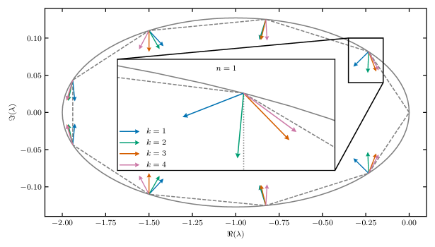
Figure 2: Fundamental directions $z_{n,k}$ of the second order correction to the eigenvalues of the asymmetric random walk with $N=9$ states and affinity $\mathcal{A}=2.3$. The unperturbed eigenvalues are connected by dashed lines. The inset shows a magnification of the first non trivial eigenvalue. All corrections point to the inside of the ellipse on which the unperturbed eigenvalues lie.

To better visualize $z_{n,k}$ in the general case, we calculate the angle on the complex plane between $z_{n,k}$ and

$$\lambda_{\perp,n}\equiv-\tanh(\mathcal{A}/(2N))\cos\left(\frac{2\pi}{N}n\right)-\mathrm{i}\sin\left(\frac{2\pi}{N}n\right)\,,$$ (41)

a complex number that is perpendicular on the ellipse and points to the inside at the position of the unperturbed eigenvalues. This angle can be written in the form

$$\phi_{n,k}=\arcsin\left(\frac{\Im(z_{n,k}\lambda_{\perp,n}^{*})}{|z_{n,k}||\lambda_{\perp,n}|}\right)$$ (42)

and depends only on the affinity and the number of states $N$. Graphical representations of the affinity-dependence of this angle are presented for different $N$ in figure 3. For better orientation the direction of the neighboring eigenvalues and the angle to the downwards direction are also plotted. It is evident that the angle is always between $-\pi/2$ and $\pi/2$ meaning that $z_{n,k}$ points inwards. For small affinities, i.e., close to equilibrium, the fundamental perturbation directions either point in positive or negative direction or along the imaginary axis, so the angles are either $\pi/2$, $-\pi/2$ or $0$. Note, however, that the non degenerate perturbation theory as it is used here is only valid for $\mathcal{A}\neq 0$, since all non-trivial eigenvalues of the master matrix for a random walk become degenerate as $\mathcal{A}$ approaches zero.

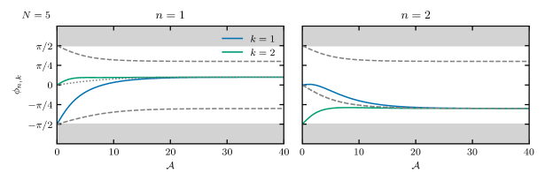
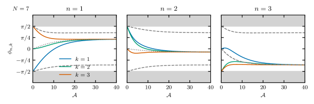
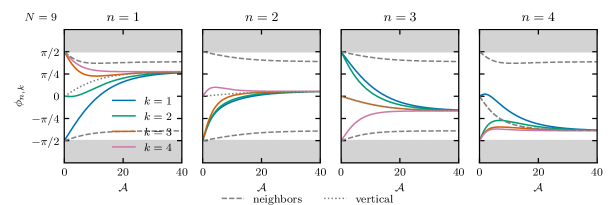
Figure 3: Angles between the fundamental directions of the second order perturbation and the direction perpendicular to the ellipse on which the unperturbed eigenvalues lie. All possible perturbations are a superposition of these directions, so the eigenvalue can only move in directions between the extremal angles. All fundamental direction form an angle between $-\pi/2$ and $\pi/2$ to the perpendicular direction, showing that there exists no perturbation that moves the eigenvalues outside of the ellipse. For better orientation the directions of the neighboring eigenvalues are indicated as dashed lines. The vertical direction is shown as a dotted line. As the affinity rises all perturbation directions converge to the vertical direction.

For large affinities $z_{n,k}$ points along the imaginary axis, since in this case $b\gg a^{2}$ holds in eq. (30), while all other terms in eq. (39) stay finite. For this reason all curves in fig. 3 collapse onto the curve indicating the vertical direction as $\mathcal{A}$ goes to infinity.

5 Numerical evidence

The asymmetric random walk has proven to be the limiting case in established bounds that depend on the affinity. In order to further substantiate the bound beyond the second order perturbation theory, in this section, we will present abundant numerical evidence for this bound in the unicyclic case by randomly generating rates that lead to a desired value of the affinity as well as numerical optimization schemes that put the conjectured bound to the test.

5.1 Randomly generated unicyclic systems

The rates for the randomly generated unicyclic networks are generated using the ansatz

$$w_{i+}=w_{i}\exp(\Delta F_{i}/2)\quad\mathrm{and}\quad w_{i-}=w_{i}\exp(-\Delta F_{i}/2)\,,$$ (43)

introducing the timescales $w_{i}$ and the free energy differences between connected states $\Delta F$. In order to achieve the desired affinity the free energy differences have to sum up to $\mathcal{A}$. For this reason, we first draw $N$ values $\Delta\tilde{F}$ independently from a uniform distribution on the interval $(-0.5,1.5)$ and calculate the energy differences as $\Delta F_{i}=\mathcal{A}\Delta\tilde{F}_{i}/\sum_{i}\Delta\tilde{F}_{i}$. The interval is asymmetrical in order to make divisions by values close to zero less likely, thereby increasing numerical stability.

The timescales $w_{i}$ are drawn from a uniform distribution between $0$ and $1$. After calculating all rates, the timescales are adjusted such that the largest exit rate takes the value $1$. For this reason the width of the interval from which the $w_{i}$ are drawn is irrelevant.

The results obtained by perturbing the asymmetric random walk show that there is a fundamental difference between systems with arbitrary exit rates (generic case) and systems that have uniform exit rates in all states. We therefore also specifically generate systems with the same exit rate in each state by rescaling the rates such that this is the case after drawing them as described above.

For each combination of $N$ and $\mathcal{A}$ that we study, we draw 10000 sets of rates both for the generic and for the case of uniform exit rates and calculate the eigenvalues of the corresponding generator. As an example the results for $N=5$ and $\mathcal{A}=1.2$ are presented in figure 5. The color indicates whether the states are drawn with random exit rates (blue) or with the same exit rate in each state (gray). Also shown are the directions of the first order perturbation according to section 4.1 and the different fundamental directions of perturbations of second order in case the first order vanishes (c.f. section 4.2).

All eigenvalues lie within the ellipse defined by the eigenvalues of the asymmetric random walk. As already conjectured in [13], the nontrivial eigenvalue with the largest real part always lies below a line connecting the origin with the first non-trivial eigenvalue of the corresponding asymmetric random walk. From the numerical data it is evident that such a relation also holds for the other eigenvalues when compared to their corresponding eigenvalue of the random walk.

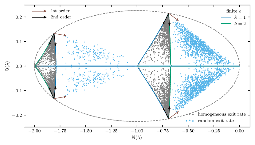
Figure 4: Scatter plot of eigenvalues for systems with $N=5$ states and $\mathcal{A}=1.2$. Random systems with unconstrained exit rates are plotted in blue. Systems with exit rates constrained to 1 are shown in gray. The solid lines show the eigenvalues of systems with rates constructed with $f_{i}^{(k)}=\cos(2\pi ik/N)$ and finite $\epsilon$. The arrows indicate the directions of the perturbation results of first and second order, respectively. From the distribution of eigenvalues it can be seen that the results obtained by perturbing the asymmetric random walk seem to extend beyond the validity of the perturbation theory in the sense that the curves corresponding to the extremal directions of the perturbation theory form approximate bounds to the eigenvalues not only in the immediate vicinity of the asymmetric random walk but for all systems with eigenvalues that have an imaginary part different from zero.

Furthermore, it is interesting to note that the results obtained through perturbation theory describe the behavior of the eigenvalues rather well, even if the system is not close to the asymmetric random walk. The eigenvalues of systems with uniform exit rate stay roughly within the cone derived from the extremal directions introduced in section 4.2. This begs the question to which extend the second order perturbation derived there constitutes a good approximation for large $\epsilon$.

To investigate this further, we calculate the eigenvalues of unicyclic systems with rates as defined in equation (25) for finite $\epsilon$ numerically. As we have seen, perturbations that correspond to the fundamental directions of the second order result are produced by the choice of $f_{i}$ such that its discrete Fourier-transform only contains one selected mode. For this reason we choose $f_{i}^{(k)}=\cos(2\pi ik/N)$. The results are shown in figure 4 as solid lines parametrized by $\epsilon\in[0,10]$. By definition these curves leave the eigenvalues in parallel to the fundamental direction corresponding to the selected Fourier mode. The curves stay approximately linear, which shows that, in this case, the perturbative result can qualitatively describe the spectrum of all systems that show oscillations and therefore have corresponding eigenvalues with nonzero imaginary part. Even for larger $\epsilon$, where the non-linearity becomes more pronounced, we see that the curves still approximately envelope the eigenvalues for randomly generated systems.

The process has been repeated for values of $N$ between $3$ and $13$ and values of $\mathcal{A}$ in the range between $0$ and $20$ with the same qualitative result (data not shown).

5.2 Numerical optimization procedure

While studying randomly generated systems can capture the generic behavior of the eigenvalues, in this section we describe a numerical method that aims to find possible violations of the conjectured bound (and fails to do so). The goal is to use standard numerical optimization algorithms to find a set of rates that produces the maximum imaginary part of a specific eigenvalue while keeping its real part fixed at a predetermined value and also obeying the constraints on affinity and exit rates.

This is done using the sequential least squares programming algorithm as it is implemented in the python library for scientific computing scipy [18], with a randomly chosen initial guess for the rates. As it is to be expected for a heavily constrained non-linear optimization problem, the algorithm converges rather poorly without case specific tweaking of the optimization parameters and the initial guess. Nevertheless it is possible to find extremal cases in some intervals of the real part, typically in the vicinity of the eigenvalues of the asymmetric random walk. The results are depicted as solid lines in figure 5. They show that the eigenvalues can not leave the ellipse defined by the random walk even if the rates are specifically designed to do so. Apparently it is not even possible to exceed the straight line connecting the origin to the corresponding eigenvalue of the asymmetric random walk, which shows once more that the results conjectured in [13] can be extended to subdominant eigenvalues.

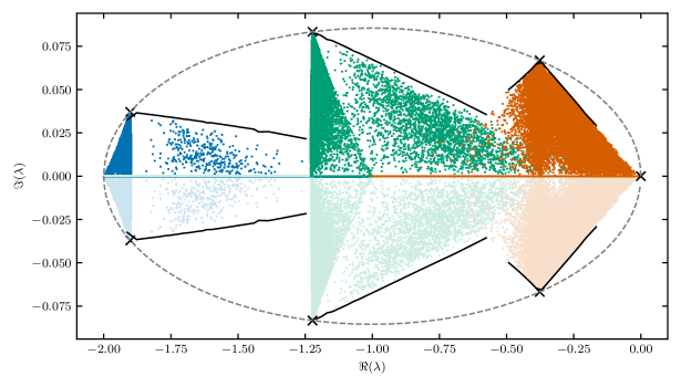
Figure 5: Scatter plot showing the eigenvalues of a cyclic Markov process with 7 states and an affinity of $\mathcal{A}=1.2$. The eigenvalues are sorted by increasing real part and are colored accordingly. Black curves show results of a numerical optimization scheme with the goal to find the process which leads to the largest (smallest) imaginary part of a specific eigenvalue with the real part fixed at a given value. Black crosses indicate the eigenvalues of the asymmetric random walk with affinity $\mathcal{A}$. The numerical results suggest that it is not possible to find a process at fixed affinity with eigenvalues that lie outside a certain region that is bounded by the ellipse on which the eigenvalues of the asymmetric random walk lie.

6 Multicyclic case

In previous studies of affinity-dependent bounds [17, 13], it turned out that the results obtained for unicyclic systems can be extended to multicyclic systems since the coupling of two or more cycles to each other can be handled by identifying the cycle that produces the weakest bound. In our case, the weakest bound is based on the cycle that maximizes the ratio $\mathcal{A}_{\mathcal{C}}/N_{\mathcal{C}}$ of cycle affinity and number of states in the cycle. In this section we provide numerical evidence that the elliptical bound can be extended to multicyclic networks following this rationale.

6.1 Simple multi cyclic network

One of the arguably simplest models to study multicyclic behavior is a network consisting of merely two fundamental cycles that share one link. Figure 6 shows an example of such a network that was previously used to illustrate universal bounds on the cumulant generating function of the distribution of entropy production (“house network”) [17]. In this section we aim to study the influence of coupled cycles on the bounds discussed above.

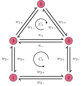
Figure 6: Schematic depiction of house network consisting of two fundamental cycles. There is a total of three possible cycles. Each cycle on its own implies an elliptical bound the eigenvalues depending on its cycle affinity. The weakest of these bounds is generated by the cycle with the maximum value of $\mathcal{A}_{\mathcal{C}}/N_{\mathcal{C}}$ and holds even the cycles are coupled.

As this example is intended to serve as a case study, we want to keep the number of different rates as low as possible, while still maintaining the possibility to fix the affinity of each cycle individually and having a meaningful parameter $\Omega$ that allows us to select which of the cycles has the dominant influence on the eigenvalues. For this reason we assume that each transition that belongs uniquely to one of the two fundamental cycles has the same forwards and backwards rates, respectively. This leaves us with 3 tuples of transition rates, $w_{1\pm}$ for transitions of cycle 1, $w_{2\pm}$ for transitions within cycle 2, and $\kappa_{\pm}$ for the transition coupling the two cycles.

We want to fix the affinities of the cycles. A suitable ansatz is

$$w_{1+} =\frac{1}{w_{0}}\exp[(\mathcal{A}_{1}-\mathcal{A}_{\mathrm{link}})/4]\quad w_{1-}=\frac{1}{w_{0}}\exp[-(\mathcal{A}_{1}-\mathcal{A}_{\mathrm{link}})/4]$$ (44)

$$w_{2+} =\frac{1}{w_{0}}\Omega\exp[(\mathcal{A}_{2}+\mathcal{A}_{\mathrm{link}})/6]\quad w_{2-}=\frac{1}{w_{0}}\Omega\exp[-(\mathcal{A}_{2}+\mathcal{A}_{\mathrm{link}})/6]$$ (45)

$$\kappa_{+} =\frac{\max\left\{1,\Omega\right\}}{w_{0}}\exp(\mathcal{A}_{\mathrm{link}}/2)\quad\kappa_{-}=\frac{\max\left\{1,\Omega\right\}}{w_{0}}\exp(-\mathcal{A}_{\mathrm{link}}/2)$$ (46)

that fixes the affinity of cycle 1 to $\mathcal{A}_{1}$ and the affinity of cycle 2 to $\mathcal{A}_{2}$. It also introduces the parameter $\Omega$ that determines the ratio between the timescales of the two cycles. The rate $w_{0}$ is chosen such that the maximum exit rate is 1. This means that if $\Omega=0$ only cycle 1 is active, while $\Omega\rightarrow\infty$ corresponds to the case in which only cycle 2 is active.

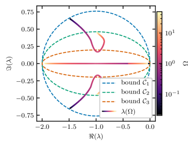
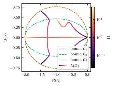
Figure 7: Eigenvalues for the house network as function of $\Omega$ for $\mathcal{A}_{1}=6$ and $\mathcal{A}_{2}=4$ (left) and $\mathcal{A}_{2}=-4$ (right) . The elliptical bounds resulting from the average link affinity in each cycle are shown as dashed lines. The parameter $\Omega$ is defined such that a value of 0 corresponds to an asymmetric random walk with affinity $\mathcal{A}_{1}$ in the upper circle and $\Omega\rightarrow\infty$ corresponds to an asymmetric random walk with an affinity $\mathcal{A}_{2}$ in the lower circle. For intermediate values the two cycles are coupled. Nonetheless the eigenvalues stay within the loosest of the three bounds.

Since we already established that the asymmetric random walk is the limiting case for unicyclic networks, it is favourable to have this case within our parameter space. This can be achieved by making the affinity of the link between the two cycles dependent on $\Omega$ in such a way that it interpolates between the values present in a random walk with 3 states and affinity $\mathcal{A}_{1}$ and a random walk with 4 states and affinity $\mathcal{A}_{2}$. A suitable choice is

$$\mathcal{A}_{\mathrm{link}}=\frac{\mathcal{A}_{1}/3+\Omega\mathcal{A}_{2}/4}{1+\Omega}\,.$$ (48)

Figure 7 shows the resulting eigenvalues as a function of $\Omega$ for the affinities $\mathcal{A}_{1}=6$ and $\mathcal{A}_{2}=\pm 4$ together with the bounds resulting from the average link affinities present in each of the three cycles. From the curves it becomes clear that coupling the two cycles ($\Omega\simeq 1$) does not drive the eigenvalues outside the loosest elliptical bound. To a certain extent the behavior of the eigenvalues can be understood intuitively. When both affinities are positive (left panel), the two cycles sustain oscillations even when coupled, since they do not compete with each other on their shared link. The two cycles behave analogously to two interlocked gears rotating in opposite directions. For this reason the imaginary part of the complex eigenvalue does not vanish for any $\Omega$. However, the situation changes when the affinities have different signs (right panel). Now, the two cycles compete over the shared link and consequently oscillations disappear for intermediary values of $\Omega$ manifesting in real valued eigenvalues.

6.2 Numerical case study

While the simple example used in section 6.1 can serve as an illustrative case study for a multi-cyclic network, it is by no means sufficient to make a claim for the generalizability of the unicyclic bound to arbitrary Markov processes. In this section we will widen the scope of our case studies to randomly generated networks with fixed number of states but randomly generated network topology.

Because the loosest bound is produced by the cycle with the largest affinity per link and the topology is random, it is rather challenging to prescribe the desired bound and then generate networks randomly that should satisfy this bound as we did in the previous case studies. Instead, we opt for the reversed approach, drawing the network first without constraints and computing the corresponding bound afterwards.

A network is generated by first drawing for each state the numbers of connections it should have from the uniform distribution of integers in the range $[2,N-1]$. This procedure guarantees that there are no dead ends and each state is part of at least one cycle. If the configuration is feasible, a graph with this configuration is generated deterministically and randomized afterwards by swapping target and source states of randomly selected connections. The specific procedure is implemented using the graph-tool python package [19]. The rates for each link are drawn from the exponential distribution

$$p(w_{i})=\exp(-w_{i})$$ (49)

Note that the overall timescale, which could be fixed using a factor in the exponent, is irrelevant in this case, since the rates are normalized afterwards such that the largest exit rate takes the value $1$.

Networks generated in this manner do, in general, not share the same elliptical bound, since the cycle affinities and even the cycles themselves are different for each network. To check whether the bound is satisfied, we iterate over all cycles contained in the network using the algorithm described in [20] and identify the maximum of $\mathcal{A}_{\mathcal{C}}/N_{\mathcal{C}}$.

We performed this procedure $10^{6}$ times for each $N$ up to 7 and did not come across a single violation of the bound. To visualize the results in a single scatter plot for a given number of states, we scale the imaginary part of the eigenvalues by a factor of $\left(\tanh\left(\mathcal{A}^{*}/N^{*}\right)\right)^{-1}$, which maps all individual bounds valid for each system to the unit circle around $-1$, thus making networks with different critical cycles comparable. Figure 8 shows the result for $N=5$. The different colors indicate the length $N^{*}$ of the cycle responsible for the bound.

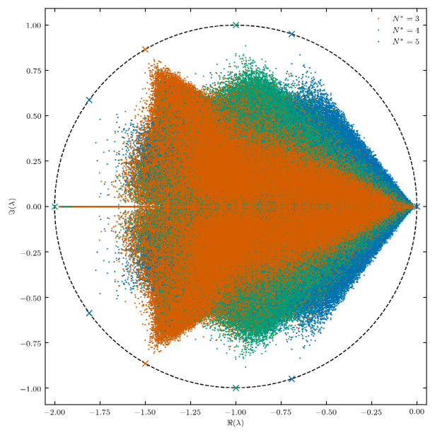
Figure 8: Scatter plot of eigenvalues of randomly generated networks with $N=5$ states. The colors encode the length $N^{*}$ of the cycle with maximum link affinity. The imaginary parts of all eigenvalues are rescaled by the factor of $(\tanh(\mathcal{A}^{*}/(2N^{*}))^{-1}$ in order to make the elliptical bounds of different networks comparable since these bounds collapse onto the unit cycle. All eigenvalues lie within the unit cycle, which allows us to conjecture that the elliptical bound is also valid in the multi cyclic case.

7 Application to time discrete Markov chains

While the term affinity is commonly used only for time continuous Markov processes, our results are not limited to this specific case. Just as the Perron-Frobenius theorem, they are equally applicable to time discrete Markov jump processes that are described by the evolution of the probability $p(i,n)$ to be in state $i$ at the discrete time step $n$ according to

$$p(i,n+1)=\sum_{j}p(i|j)p(j,n)$$ (50)

with the transition probability $p(i|j)$.

The definition of the affinity of a cycle translates to the logarithmic ratio of the probability to observe a forward trajectory along this cycle and the probability to observe the time-reversed one, i.e.,

$$\mathcal{A}_{\mathrm{disc}}=\sum_{i\rightarrow j}\ln\left(\frac{p(j|i)}{p(i|j)}\right)\,,$$ (51)

where the sum runs over all links from $i$ to $j$ of the specific cycle.

The eigenvalues of the propagator of a unicylic system with equal forward and backward jump probability, respectively that is the counterpart of a time continuous random walk, are given by

$$\lambda_{\mathrm{disc},n}=\lambda_{n}^{(0)}/w_{0}+1=\cos(2\pi n/N)+\mathrm{i}\tanh(\mathcal{A}/2N)\sin(2\pi n/N)\,.$$ (52)

In regards to the elliptical bound, the treatment of time discrete processes has the advantage that the timescale, which is explicitly present as $w_{0}$ in the time continuous case, is inherently fixed by the discreteness of the process. As a result, the bound does no longer rely on the knowledge of a parameter other than the affinity per state, which could prove useful for inferring the discrete affinity from measurements of correlation functions.

In a similar way, the results obtained here could be generalized to arbitrary mathematical spectral problems of non-negative matrices, although the quantity that serves as the effective affinity in these cases may not have a physical interpretation as it is the case for Markovian systems.

8 Conclusion

We studied the intricate connection between the spectrum of generators of time continuous Markovian dynamics and the affinity, a measure for breaking time reversal symmetry. Based on extensive numerical case studies and results obtained from perturbation theory, we conjecture that the eigenvalues of such generators can be constrained by the ellipse on which the eigenvalues of a corresponding asymmetric random walk lie.

While we could not provide a rigorous proof for the conjecture, our results obtained for perturbations of the asymmetric random walk became a formal proof if it was possible to show that a unicyclic process with homogeneous rates is the only process with eigenvalues on the conjectured elliptical bound.

The presented results show once again that for many aspects that involve non-equilibrium systems, affinity-dependent bounds can be obtained by comparing the system with the corresponding asymmetric random walk with the same affinity per state. This strategy has already proven useful in deriving affinity-dependent bounds on distributions of stochastic currents of which the thermodynamic uncertainty relation is the most prominent example.

Besides a rigorous proof of the conjecture put forth in this work, the most pressing open question is whether there is an underlying connection between these results that would explain why the asymmetric random walk appears time and time again as the limiting case when quantifying the influence of the distance from equilibrium to certain physical quantities.

Appendix A Perturbation theory of normal matrices

Since generic master generators are not Hermitian and their eigenvectors are therefore in general not pairwise orthogonal, the formulas of time independent perturbation theory, as they are known from quantum mechanics, are not directly applicable to these matrices. In the case of an asymmetric random walk, however, the corresponding matrix is normal, i. e.,

$$\left[\mathbf{M}^{(0)},{\mathbf{M}^{(0)}}^{\dagger}\right]=0\,.$$ (53)

As a consequence, the eigenvectors of $\mathbf{M}^{(0)}$ form an orthonormal basis of the corresponding Hilbert space. The aim of this section is to re-derive known results from quantum mechanics using only the normal property of the perturbed matrix.

By virtue of being normal, the generator $\mathbf{M}^{(0)}$ of an asymmetric random walk satisfies the relations

$$\braket{\nu_{n}^{0}}{\nu_{n^{\prime}}^{0}} =\delta_{n,n^{\prime}}$$ (54)

$$\mathbf{M}^{(0)}\ket{\nu_{n}^{0}} =\lambda_{n}\ket{\nu_{n}^{0}}$$ (55)

$${\mathbf{M}^{(0)}}^{\dagger}\ket{\nu_{n}^{0}} =\lambda_{n}^{*}\ket{\nu_{n}^{0}}\,.$$ (56)

We want to calculate the eigenvalues $\lambda_{n}$ and the normalized eigenvectors $\ket{\nu^{n}}$ of the perturbed matrix

$$\mathbf{M}=\mathbf{M}^{(0)}+\epsilon\mathbf{M}^{(1)}$$ (57)

up to second order in $\epsilon$, i.e., we calculate a perturbative solution to the eigenvalue equation

$$(\mathbf{M}-\lambda_{n})\ket{\nu_{n}}=0$$ (58)

Since the eigenvectors of the unperturbed problem form an orthornormal basis, it is possible to express the perturbed eigenvector as a superposition of these, such that we can write

$$\ket{\nu_{n}}=c_{n}\ket{\nu_{n}^{0}}+\sum_{m\neq n}d_{m}\ket{\nu_{m}^{0}}\,,$$ (59)

where the coefficients $d_{m}$ are of the order $\epsilon$.

The normalization condition of eigenvectors leads therefore to

$$\braket{\nu_{n}}{\nu_{n}}=1\quad\Leftrightarrow\quad|c_{n}|^{2}+\sum_{m\neq n}|d_{m}|^{2}=1$$ (60)

which results in $c_{n}=1-\mathcal{O}(\epsilon^{2})$.

By inserting these results into the eigenvalue equation we obtain

$$\left(\mathbf{M}-\lambda_{n}\right)\ket{\nu_{n}^{0}}=(\mathbf{M}^{(0)}+\epsilon\mathbf{M}^{(1)}-\lambda_{n})\left[\ket{\nu_{n}^{0}}+\sum_{m\neq n}d_{m}\ket{\nu_{m}^{0}}\right]+\mathcal{O}(\epsilon^{2})$$ (61)

Projection of this equation onto an eigenvector $\ket{\nu_{n^{\prime}}^{0}}$ with $n^{\prime}\neq n$ leads to

$$\braket{\nu_{n^{\prime}}^{0}}{\mathbf{M}-\lambda_{n}}{\nu_{n}^{0}}=\epsilon\braket{\nu_{n^{\prime}}^{0}}{M_{1}}{\nu_{n}^{0}}+\sum_{m\neq n}d_{m}\left[\lambda_{m}^{0}\delta_{m,n^{\prime}}+\epsilon\braket{\nu_{n^{\prime}}^{0}}{\mathbf{M}^{(1)}}{\nu_{m}^{0}}\!-\!\lambda_{n}\delta_{m,n^{\prime}}\right]\mathop{\kern 0.0pt\mbox{=}}\limits^{\mbox{\scriptsize!}}0$$ (62)

The leading order of this equation in $\epsilon$ reads

$$\epsilon\braket{\nu_{n^{\prime}}^{0}}{\mathbf{M}^{(1)}}{\nu_{n}^{0}}+d_{n^{\prime}}\left(\lambda_{n^{\prime}}^{0}-\lambda_{n}\right)=0$$ (63)

from which we readily obtain the leading order of the coefficients as

$$d_{n^{\prime}} =\epsilon\frac{\braket{\nu_{n^{\prime}}^{0}}{\mathbf{M}^{(1)}}{\nu_{n}^{0}}}{\lambda_{n}-\lambda_{n^{\prime}}^{0}}+\mathcal{O}(\epsilon^{2})$$ (64)

$$=\epsilon\frac{\braket{\nu_{n^{\prime}}^{0}}{\mathbf{M}^{(1)}}{\nu_{n}^{0}}}{\lambda_{n}^{0}-\lambda_{n^{\prime}}^{0}}+\mathcal{O}(\epsilon^{2})\,.$$

Here we could replace $\lambda_{n}$ with $\lambda_{n}^{0}$ in the second step since the difference of the two is of order $\epsilon$ and therefore negligible in the leading order.

By projection of eq. (61) onto $\ket{\nu_{n}^{0}}$ and by using the results form (64), it is now possible to solve for the corrections to the eigenvalues up to order $\epsilon^{2}$

$$0=\bra{\nu_{n}^{0}}\left(\mathbf{M}^{(0)}+\epsilon\mathbf{M}^{(1)}-\lambda_{n}\right)\left(\ket{\nu_{n}^{0}}+\epsilon\sum_{m\neq n}\frac{\braket{\nu_{m}^{0}}{\mathbf{M}^{(1)}}{\nu_{n}^{0}}}{\lambda_{n}^{0}-\lambda_{m}^{0}}\ket{\nu_{m}^{0}}+\mathcal{O}(\epsilon^{2})\right)\\$$ (65)

Solving for $\lambda_{n}$ finally yields

$$\lambda_{n}=\lambda_{n}^{0}+\epsilon\braket{\nu_{n}^{0}}{\mathbf{M}^{(1)}}{\nu_{n}^{0}}+\epsilon^{2}\sum_{m\neq n}\frac{\braket{\nu_{n}^{0}}{\mathbf{M}^{(1)}}{\nu_{m}^{0}}\braket{\nu_{m}^{0}}{\mathbf{M}^{(1)}}{\nu_{n}^{0}}}{\lambda_{n}^{0}-\lambda_{m}^{0}}+\mathcal{O}(\epsilon^{3})$$ (66)

which resembles closely the result used in quantum mechanics; the only difference being that in this more general case the matrix elements and eigenvalues can be complex.

References

References

- [1] Agaev R and Chebotarev P 2005 Linear Algebra and its Applications 399 157–168
- [2] Meyer C D 2000 Matrix analysis and applied linear algebra (Philadelphia: Society for Industrial and Applied Mathematics) ISBN 978-0-89871-454-8 oCLC: 702199335
- [3] Maroulas J, Psarrakos P J and Tsatsomeros M J 2002 Linear Algebra and its Applications 348 49–62
- [4] Pillai S U, Suel T and Seunghun Cha 2005 IEEE Signal Processing Magazine 22 62–75
- [5] Seifert U 2019 Annu. Rev. Condens. Matter Phys. 10 171–192
- [6] Barato A C and Seifert U 2015 Phys. Rev. Lett. 114 158101
- [7] Gingrich T R, Horowitz J M, Perunov N and England J L 2016 Phys. Rev. Lett. 116 120601
- [8] Horowitz J M and Gingrich T R 2017 Phys. Rev. E 96 020103
- [9] Proesmans K and Van den Broeck C 2017 EPL 119 20001
- [10] Fei C, Cao Y, Ouyang Q and Tu Y 2018 Nature Communications 9 1434
- [11] Nguyen B, Seifert U and Barato A C 2018 J. Chem. Phys. 149 045101
- [12] Owen J A, Kolchinsky A and Wolpert D H 2019 New J. Phys. 21 013022
- [13] Barato A C and Seifert U 2017 Phys. Rev. E 95 062409
- [14] Dmitriev N and Dynkin E 1945 C.R. (Dokl.) Acad.Sci. URSS (N.S.) 49 159–162
- [15] Dmitriev N and Dynkin E 1946 Izvestia Akad. Nauk SSSR Ser. Mat. 10 167–184
- [16] Swift J 1972 Location of Characteristic Roots of Stochastic Matrices Master Thesis McGill University Montreal
- [17] Pietzonka P, Barato A C and Seifert U 2016 Phys. Rev. E 93 052145
- [18] Kraft D 1988 A software package for sequential quadratic programming Tech. Rep. DFVLR-FB 88-28 DLR German Aerospace Center – Institute for Flight Mechanics, Kön, Germany oCLC: 27846848
- [19] Peixoto T P 2017 The graph-tool python library figshare
- [20] Hawick K A and James H A 2008 Enumerating Circuits and Loops in Graphs with Self-Arcs and Multiple-Arcs Proc. 2008 Int. Conf. on Foundations of Computer Science (FCS’08) (Las Vegas, USA: CSREA / Massey University) pp 14–20