Primordial black holes from the preheating instability in single-field inflation

Abstract

After the end of inflation, the inflaton field oscillates around a local minimum of its potential and decays into ordinary matter. These oscillations trigger a resonant instability for cosmological perturbations with wavelengths that exit the Hubble radius close to the end of inflation. In this paper, we study the formation of Primordial Black Holes (PBHs) at these enhanced scales. We find that the production mechanism can be so efficient that PBHs subsequently dominate the content of the universe and reheating proceeds from their evaporation. Observational constraints on the PBH abundance also restrict the duration of the resonant instability phase, leading to tight limits on the reheating temperature that we derive. We conclude that the production of PBHs during reheating is a generic and inevitable property of the simplest inflationary single-field models, and does not require any fine tuning of the inflationary potential.

1 Introduction

The reheating stage [1, 2, 3, 4] is a crucial part of the inflationary scenario [5, 6, 7, 8, 9]. It allows inflation to come to an end, and describes how the inflaton field decays and produces ordinary matter. Although reheating appears to be a rather complicated process, as far as the large scales probed by the Cosmic Microwave Background (CMB) anisotropies are concerned [10, 11], the influence of this epoch on the predictions of inflation is simple, at least in single-field models. This is due to the fact that, on large scales, the curvature perturbation is conserved [12, 13], which implies that the details of the reheating process do not affect the inflationary predictions. In fact, those predictions are sensitive to a single parameter, the so-called reheating parameter [14], which is a combination of the reheating temperature and of the mean equation-of-state parameter, and which determines the location of the observational window along the inflationary potential. Given the restrictions on the shape of the potential now available [15, 16, 17, 18, 19], this can be used to constrain reheating [20, 21, 22, 23].

On small scales however, the situation is different. It was indeed shown in LABEL:Jedamzik:2010dq (see also LABEL:Easther:2010mr) that, for scales leaving the Hubble radius during the last $\sim 10$ e-folds of inflation (if the energy scale of inflation is not tuned to extremely low values), there is a parametric instability that can lead to an enormous growth of perturbations. This can cause early structure formation and/or gravitational waves production [24, 25, 26], and may open a new observational window on inflation and reheating.

In the present paper, we study yet another possible consequence of the presence of this instability, namely the production of Primordial Black Holes (PBHs) [27, 28]. The motivation is twofold. First, this may lead to a new inflationary mechanism for black hole production which is completely natural and generic. Usually, it is necessary to consider very specific potentials in order for this production to be efficient. In this work, the only assumption is that the potential can be approximated by a parabola around its minimum. Except for fine-tuned situations (where, for instance, a symmetry prevents the presence of a quadratic term in the Taylor expansion of the potential about its minimum), this is always the case. Second, tight constraints on the abundance of PBHs have been placed in various mass ranges (for a review, see e.g. Refs. [29, 30]), and this can be used to obtain extra information about the reheating epoch. Note that PBH formation during preheating has been studied in Refs. [31, 32, 33, 34], although in a different context.

The paper is organised as follows. In the next section, Sec. 2, we briefly review LABEL:Jedamzik:2010dq and the physical mechanism that leads to the instability mentioned above. Then, in Sec. 3, we study under which physical conditions PBHs are formed. In Sec. 3.1, based on LABEL:Goncalves:2000nz, we derive the critical density contrast from the requirement that the instability must last long enough, before reheating is completed, to allow the initial scalar field overdensity to form a black hole. In Sec. 3.2, the corresponding criterion is refined by taking Hawking evaporation into account. We then calculate the mass fraction at the end of the instability phase in Sec. 3.3. Due to the high efficiency of the instability, we find that the corresponding values for the fraction of the universe comprised in PBHs can be larger than one, which is not possible. The mass fraction must therefore be renormalised, which is done in Sec. 3.4. We propose two ways to carry out this procedure, one which accounts for the possible inclusion of PBHs within larger ones (Sec. 3.4.1), and one which accounts for the premature termination of the instability phase by the backreaction of PBHs (Sec. 3.4.2). Having calculated the abundance of PBHs at the end of the instability, in Sec. 3.5, we proceed with calculating their abundance in the subsequent radiation-dominated epoch. In some cases, we find that PBHs are so abundant that the radiation-dominated era is delayed and we discuss under which conditions this occurs in Sec. 3.6. In Sec. 3.7, we also consider the case where black holes do not entirely evaporate but leave Planckian relics behind. In Sec. 4, we derive the observational consequences of the above-described mechanism. In Sec. 4.1, we establish restrictions on the energy density at the onset of the radiation dominated era (the reheating temperature). From current constraints on PBHs (Sec. 4.2) and Planckian relics (Sec. 4.3) abundances, we then derive constraints on the energy scale of inflation and the reheating temperature. In Sec. 5, we summarise our main results and present our conclusions. Finally, the paper ends with two appendices. In Appendix A, we explain how a scalar field (here, the inflaton field) can collapse and form a black hole and, in Appendix B, we use these considerations to derive the expression of the critical density contrast used in the rest of the paper.

2 Inflation and the preheating instability

We consider scenarios where inflation is realised by a single scalar field $\phi$ (the inflaton), which slowly rolls down its potential $V(\phi)$ and then oscillates at the bottom of it. In flat Friedmann-Lemaître-Robertson-Walker space-times, the dynamics of the homogeneous inflaton field is driven by the Klein-Gordon and the Friedmann equations,

$$\ddot{\phi}+3H\dot{\phi}+V^{\prime}\left(\phi\right)=0\,,\quad H^{2}=\dfrac{V\left(\phi\right)+\dfrac{\dot{\phi}^{2}}{2}}{3M_{\scriptscriptstyle{\mathrm{Pl}}}^{2}}\,.$$ (2.1)

Hereafter, $H=\dot{a}/a$ is the Hubble parameter, $a(t)$ is the scale factor, a dot denotes derivative with respect to cosmic time, and $M_{\scriptscriptstyle{\mathrm{Pl}}}$ is the reduced Planck mass. These equations can be solved numerically or with the help of the slow-roll approximation, and the solution is insensitive to the choice of initial conditions due to the presence of the slow-roll attractor [36, 37, 38, 39, 40]. Inflation ends when the first slow-roll parameter $\epsilon_{1}\equiv-\dot{H}/H^{2}$ reaches one; then, starts the reheating/preheating phase.

Close to its minimum, we assume the potential to be approximated by a quadratic function,

$$V\left(\phi\right)=\frac{m^{2}}{2}\phi^{2}.$$ (2.2)

When, after the end of inflation, the inflaton field explores this part of the potential, $H\ll m$ and $\phi$ behaves as

$$\phi(t)\simeq\phi_{0}\left(\frac{a_{0}}{a}\right)^{3/2}\sin\left(mt\right).$$ (2.3)

This implies that the energy density stored in $\phi$ redshifts on average as matter [1], $\rho_{\phi}\propto a^{-3}$, and that the oscillations have a frequency given by the mass $m$. Here, the subscript “$0$” just denotes a reference time that might be taken at the end of inflation. Let us stress that we only assume the inflationary potential to be of the quadratic form towards the end of inflation, see footnote 1. No restriction on its shape is imposed at the scales where the cosmological perturbations observed in the CMB are produced, where the potential can e.g. be of the plateau type, and provide a good fit to observations. This means that the parameter $m$ in Eq. (2.2) should not be fixed to match the CMB power spectrum amplitude as usually done, but should be left free in order to scan different values of $H_{\mathrm{end}}$, namely different energy scales at the end of inflation. In practice, this can be done as follows. Inflation ends when $\phi_{\mathrm{end}}\simeq 1.0092M_{\scriptscriptstyle{\mathrm{Pl}}}$. Given that $\epsilon_{1}=3\dot{\phi}^{2}/2/(V+\dot{\phi}^{2}/2)$, at the end of inflation, $\dot{\phi}^{2}=V$, and one can relate $H_{\mathrm{end}}$ to $m$ according to

$$m=2H_{\mathrm{end}}\frac{M_{\scriptscriptstyle{\mathrm{Pl}}}}{\phi_{\mathrm{end}}}\,.$$ (2.5)

In this way, by varying $m$ one can vary the value of the Hubble parameter at the end of inflation, $H_{\mathrm{end}}$.

For the cosmological perturbations, there is a single gauge-invariant scalar degree of freedom that can be described with the Mukhanov-Sasaki variable [12, 13] $v$, which is a combination of the perturbed inflaton field and of the Bardeen potential, the latter being a generalisation of the gravitational Newtonian potential [41]. Its Fourrier component $v_{\bm{k}}$ evolves according to [42]

$$v_{\bm{k}}^{\prime\prime}+\left(k^{2}-\frac{z^{\prime\prime}}{z}\right)v_{\bm{k}}=0,$$ (2.6)

where a prime denotes a derivative with respect to conformal time $\eta$, defined as $\mathrm{d}t=a\mathrm{d}\eta$. In this expression, $z\equiv\mathchoice{{\hbox{$\displaystyle\sqrt{2\epsilon_{1}\,}$}\lower 0.4pt\hbox{\vrule height=6.44444pt,depth=-5.15558pt}}}{{\hbox{$\textstyle\sqrt{2\epsilon_{1}\,}$}\lower 0.4pt\hbox{\vrule height=6.44444pt,depth=-5.15558pt}}}{{\hbox{$\scriptstyle\sqrt{2\epsilon_{1}\,}$}\lower 0.4pt\hbox{\vrule height=4.51111pt,depth=-3.6089pt}}}{{\hbox{$\scriptscriptstyle\sqrt{2\epsilon_{1}\,}$}\lower 0.4pt\hbox{\vrule height=3.22221pt,depth=-2.57779pt}}}aM_{\scriptscriptstyle{\mathrm{Pl}}}$ and is such that

$$\frac{z^{\prime\prime}}{z}=a^{2}H^{2}\left[\left(1+\frac{\epsilon_{2}}{2}\right)\left(2-\epsilon_{1}+\frac{\epsilon_{2}}{2}\right)+\frac{\epsilon_{2}\epsilon_{3}}{2}\right]\,,$$ (2.7)

where $\epsilon_{2}\equiv\mathrm{d}\ln\epsilon_{1}/\mathrm{d}N$ and $\epsilon_{3}\equiv\mathrm{d}\ln\epsilon_{2}/\mathrm{d}N$ are the second and the third slow-roll parameters respectively. The initial condition is taken in the Bunch-Davies vacuum, i.e. such that $v_{\bm{k}}\rightarrow e^{-ik\eta}/\mathchoice{{\hbox{$\displaystyle\sqrt{2k\,}$}\lower 0.4pt\hbox{\vrule height=6.94444pt,depth=-5.55559pt}}}{{\hbox{$\textstyle\sqrt{2k\,}$}\lower 0.4pt\hbox{\vrule height=6.94444pt,depth=-5.55559pt}}}{{\hbox{$\scriptstyle\sqrt{2k\,}$}\lower 0.4pt\hbox{\vrule height=4.8611pt,depth=-3.8889pt}}}{{\hbox{$\scriptscriptstyle\sqrt{2k\,}$}\lower 0.4pt\hbox{\vrule height=3.47221pt,depth=-2.77779pt}}}$ when $k\gg aH$, and the function $z^{\prime\prime}/z$ is evaluated on the background dynamics that has been numerically integrated as explained above. In this way, one can compute the amplitude of $v_{\bm{k}}$ at the end of inflation for each mode $k$.

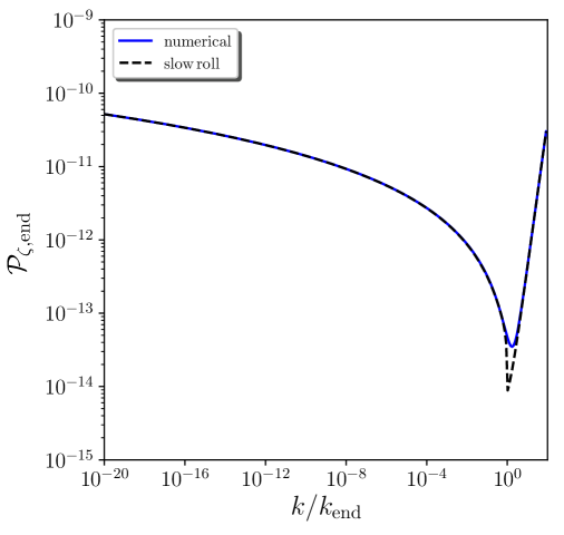
Figure 1: Power spectrum of the curvature perturbation at the end of inflation for $m\simeq 1.14\times 10^{-6}\,M_{\scriptscriptstyle{\mathrm{Pl}}}$, corresponding to $\rho_{\mathrm{inf}}\equiv 3H_{\mathrm{end}}^{2}M_{\scriptscriptstyle{\mathrm{Pl}}}^{2}=10^{-12}M_{\scriptscriptstyle{\mathrm{Pl}}}^{4}\simeq\left(2.43\times 10^{15}\mathrm{GeV}\right)^{4}$, as a function of $k/k_{\mathrm{end}}$, where $k_{\mathrm{end}}$ is the scale that exits the Hubble radius at the end of inflation. The blue solid line corresponds to the numerical solution of Eq. (2.6) while the black dashed line stands for the slow-roll approximation (2.8).

It is convenient to introduce the curvature perturbation $\zeta$ defined as $\zeta=v/z$ since this quantity is conserved on super-Hubble scales, and to compute the power spectrum $\mathcal{P}_{\zeta}=k^{3}|\zeta_{\bm{k}}|^{2}/(2\pi^{2})$ of that quantity at the end of inflation. It is displayed in Fig. 1 for the value of $m$ corresponding to $\rho_{\mathrm{inf}}\equiv 3H_{\mathrm{end}}^{2}M_{\scriptscriptstyle{\mathrm{Pl}}}^{2}=10^{-12}M_{\scriptscriptstyle{\mathrm{Pl}}}^{4}\simeq\left(2.43\times 10^{15}\mathrm{GeV}\right)^{4}$, as a function of $k/k_{\mathrm{end}}$, where $k_{\mathrm{end}}=a_{\mathrm{end}}H_{\mathrm{end}}$ is the scale that exits the Hubble radius at the end of inflation, see also Fig. 2. The blue solid line corresponds to the numerical solution of Eq. (2.6), while the black dashed line stands for the slow-roll approximated solution of that equation, namely [43, 44]

$$\mathcal{P}_{\zeta,\mathrm{end}}=\begin{cases}\dfrac{H_{*}^{2}\left(k\right)}{8\pi^{2}M_{\scriptscriptstyle{\mathrm{Pl}}}^{2}\epsilon_{1*}\left(k\right)}\left[1+\left(\dfrac{k}{k_{\mathrm{end}}}\right)^{2}\right]\left[1-2\left(C+1\right)\epsilon_{1*}\left(k\right)-C\epsilon_{2*}\left(k\right)\right]\ \text{if}\ k<k_{\mathrm{end}}\\ \dfrac{H_{\mathrm{end}}^{2}}{8\pi^{2}M_{\scriptscriptstyle{\mathrm{Pl}}}^{2}}\left[1+\left(\dfrac{k}{k_{\mathrm{end}}}\right)^{2}\right]\ \text{if}\ k>k_{\mathrm{end}}\end{cases}.$$ (2.8)

In this expression, for the modes that cross out the Hubble radius before the end of inflation, $k<k_{\mathrm{end}}$, the functions $H_{*}(k)$, $\epsilon_{1*}(k)$ and $\epsilon_{2*}(k)$ respectively denote the values of $H$, $\epsilon_{1}$ and $\epsilon_{2}$ at the time when the mode $k$ exits the Hubble radius, and are evaluated in the numerical solution of Eqs. (2.1). The parameter $C\simeq-0.7296$ is a numerical constant. One can check in Fig. 1 that, except for the very few modes that are close to the Hubble scale at the end of inflation and for which the amount of power is underestimated, Eq. (2.8) provides a very good fit to the numerical solution.

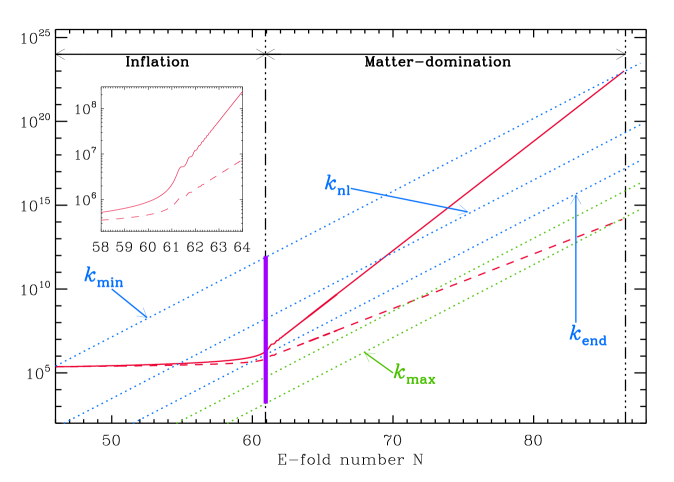
Figure 2: Evolution of the relevant physical scales versus the e-folds number. The continuous red line denotes the Hubble radius, which is also the upper bound of the instability band, while the dashed red line represents the scale $\textstyle\sqrt{3Hm\,}$  which corresponds to the lower bound of the resonance band. The dotted lines represent the physical wavelengths of different Fourier modes: the “green modes” enter the instability mode from below while the “blue modes” enter it from above. The inset shows the detailed behaviours of the Hubble radius and $\textstyle\sqrt{3Hm\,}$  at the transition between inflation and reheating. Figure taken from LABEL:Jedamzik:2010dq.

As already mentioned, after the end of inflation, the inflaton oscillates at the bottom of its quadratic potential and the evolution of the perturbations through this epoch strongly depends on the scales considered. On large scales (for instance, CMB scales), the conservation of curvature perturbation is sufficient to establish that the power spectrum (2.8) calculated at the end of inflation propagates through the reheating epoch without being distorted. However, on small scales, things can be very different. As shown in LABEL:Jedamzik:2010dq, for modes satisfying

$$aH<k<a\mathchoice{{\hbox{$\displaystyle\sqrt{3Hm\,}$}\lower 0.4pt\hbox{\vrule height=6.83331pt,depth=-5.46667pt}}}{{\hbox{$\textstyle\sqrt{3Hm\,}$}\lower 0.4pt\hbox{\vrule height=6.83331pt,depth=-5.46667pt}}}{{\hbox{$\scriptstyle\sqrt{3Hm\,}$}\lower 0.4pt\hbox{\vrule height=4.78333pt,depth=-3.82668pt}}}{{\hbox{$\scriptscriptstyle\sqrt{3Hm\,}$}\lower 0.4pt\hbox{\vrule height=3.41666pt,depth=-2.73334pt}}},$$ (2.9)

see Fig. 2, the oscillations source a parametric resonance (in the narrow resonance regime). The reason is that, thanks to these oscillations, Eq. (2.6) becomes a Mathieu equation and the condition (2.9) is in fact equivalent to being in the first instability band of that equation. We see that the instability occurs if the physical wavelength of a mode is smaller than the Hubble radius (continuous red line in Fig. 2) during reheating and larger than a new scale given by $\textstyle\sqrt{3Hm\,}$  (dashed red line in Fig. 2). Moreover, two types of mode can be distinguished. The “blue modes” in Fig. 2 exit the Hubble radius during inflation and re-enter it during reheating; these modes therefore enter the instability band from above. On the other hand, the “green modes” never exit the Hubble radius and enter the instability band from below by crossing the new scale $\textstyle\sqrt{3Hm\,}$ . Once within the instability band, as described in LABEL:Jedamzik:2010dq, the fluctuations get strongly amplified, such that the density contrast grows linearly with the scale factor. Effectively, they thus behave as pressureless matter perturbations in a pressureless matter universe. In what follows, this epoch is referred to as the “instability phase”. As explained in Sec. 1, during this epoch, cosmological perturbations at the amplified scales may collapse into PBHs. When the inflaton decays into other degrees of freedom (or when the PBHs take the inflaton over, see below), the instability stops, and the density of black holes evolves under various physical effects (cosmic expansion, Hawking evaporation, accretion, merging, etc.).

Let us further discuss the quadratic approximation for the inflationary potential. The largest scales amenable to parametric resonance during the instability phase are such that $k=a_{\mathrm{instab}}H_{\mathrm{instab}}$, where the time $t_{\mathrm{instab}}$ denotes the end of the instability phase (the corresponding Fourier mode is denoted “$k_{\mathrm{min}}$” in Fig. 2). During inflation, they cross out the Hubble radius at a number of e-folds $\sim\ln(H_{\mathrm{end}}/H_{\mathrm{instab}})/3$ before the end of inflation, where we recall that $H_{\mathrm{end}}$ is the value of the Hubble parameter at the end of inflation and where we have used that, during the instability, the universe is matter dominated at the background level. Since observational bounds on the tensor-to-scalar ratio impose [11] $H_{\mathrm{end}}<8\times 10^{13}\,\mathrm{GeV}$, and given that $H_{\mathrm{instab}}>H_{\mathrm{BBN}}\sim(10\,\mathrm{MeV})^{2}/\mathchoice{{\hbox{$\displaystyle\sqrt{3M_{\scriptscriptstyle{\mathrm{Pl}}}^{2}\,}$}\lower 0.4pt\hbox{\vrule height=8.63776pt,depth=-6.91023pt}}}{{\hbox{$\textstyle\sqrt{3M_{\scriptscriptstyle{\mathrm{Pl}}}^{2}\,}$}\lower 0.4pt\hbox{\vrule height=8.63776pt,depth=-6.91023pt}}}{{\hbox{$\scriptstyle\sqrt{3M_{\scriptscriptstyle{\mathrm{Pl}}}^{2}\,}$}\lower 0.4pt\hbox{\vrule height=6.0722pt,depth=-4.85779pt}}}{{\hbox{$\scriptscriptstyle\sqrt{3M_{\scriptscriptstyle{\mathrm{Pl}}}^{2}\,}$}\lower 0.4pt\hbox{\vrule height=4.70554pt,depth=-3.76445pt}}}\sim 10^{-23}\,\mathrm{GeV}$, where hereafter “BBN” stands for big-bang nucleosynthesis, this number of e-folds needs to be smaller than $\sim 28$. All the scales of interest for the problem at hand are therefore generated in the last $28$ e-folds of inflation, where we assume the potential to be well approximated by the quadratic form (2.2). Although one may be suspicious that this approximation holds for $28$ e-folds, let us stress that this value is in fact an extreme upper bound that comes from saturating the condition $H_{\mathrm{instab}}>H_{\mathrm{BBN}}$, while we will see below that most of the relevant parameter space is such that $H_{\mathrm{instab}}$ and $H_{\mathrm{BBN}}$ are separated by many orders of magnitude and this number of e-folds is in fact much smaller. In practice, potentials favoured by the data (such as plateau ones) tend to be shallower than the quadratic one away from the end of inflation, and we have explicitly checked that this approximation only slightly underestimates the amplitude of scalar perturbations in such potentials, leading to conservative statements regarding the amount of PBHs. It is nonetheless clear that the calculational program laid out below can easily be performed for any given potential, such that the approximation (2.2) for the last e-folds of inflation is released. In this work, it however allows us to carry out a full parameter-space analysis, where the energy scale of inflation can be varied without relying on a specific potential. We will see that this provides an overall picture where several interesting regions are identified, in which a more detailed analysis can always be carried out.

3 PBH formation during reheating

We have just seen that the modes in the resonance band (2.9) behave as pressureless matter fluctuations in a pressureless matter universe. In Ref. [35] and in the two appendices, see Eq. (B.7), it is shown that they collapse into PBHs after a time [35]

$$\Delta t_{\mathrm{collapse}}=\frac{\pi}{H\left[t_{\mathrm{bc}}(k)\right]\delta_{\bm{k}}^{3/2}\left[t_{\mathrm{bc}}(k)\right]},$$ (3.1)

where $t_{\mathrm{bc}}(k)$ denotes the “band-crossing” time, i.e. the time at which the mode $k$ crosses in the instability band (2.9).

Let us note that, in a matter-dominated universe, $aH$ decreases as $a^{-1/2}$ while $a\mathchoice{{\hbox{$\displaystyle\sqrt{H\,}$}\lower 0.4pt\hbox{\vrule height=6.83331pt,depth=-5.46667pt}}}{{\hbox{$\textstyle\sqrt{H\,}$}\lower 0.4pt\hbox{\vrule height=6.83331pt,depth=-5.46667pt}}}{{\hbox{$\scriptstyle\sqrt{H\,}$}\lower 0.4pt\hbox{\vrule height=4.78333pt,depth=-3.82668pt}}}{{\hbox{$\scriptscriptstyle\sqrt{H\,}$}\lower 0.4pt\hbox{\vrule height=3.41666pt,depth=-2.73334pt}}}$ increases as $a^{1/4}$, so the bounds defining the instability band (2.9) are such that, when a mode crosses in the band, it remains in the band (in other words, modes cannot cross out the band).

This instability stops when the coherent oscillations of the inflaton are over. This can happen e.g. when the inflaton decays into other fields. In the case of perturbative preheating, this occurs when the Hubble parameter drops below the decay rate $\Gamma$ of the inflaton, and for this reason, hereafter this time is referred to as $t_{\Gamma}$. One should however note that the results derived below are independent of the precise way in which the phase of coherent oscillations stop, since the time at which this happens (regardless of the way it happens) is simply one of the parameters in the present scenario.

Let us also stress that, for later convenience, we have introduced the two notations $t_{\mathrm{instab}}$ and $t_{\Gamma}$. As mentioned above, $t_{\mathrm{instab}}$ denotes the end of the instability while $t_{\Gamma}$ denotes the time at which the field decays. Although they are identical in the standard picture, we will see below that there are cases where they differ (for instance if PBHs come to dominate the universe content before the inflaton decays), which explains the need for two distinct notations.

3.1 Formation criterion

Let us now determine under which conditions PBHs form. The last mode to enter the band (2.9) “from above” is such that $k=a_{\Gamma}H_{\Gamma}$, which leads to $k/k_{\mathrm{end}}=(\rho_{\Gamma}/\rho_{\mathrm{inf}})^{1/6}$. The last mode that enters the band “from below” is, on the other hand, such that $k=a_{\Gamma}\mathchoice{{\hbox{$\displaystyle\sqrt{3H_{\Gamma}m\,}$}\lower 0.4pt\hbox{\vrule height=6.83331pt,depth=-5.46667pt}}}{{\hbox{$\textstyle\sqrt{3H_{\Gamma}m\,}$}\lower 0.4pt\hbox{\vrule height=6.83331pt,depth=-5.46667pt}}}{{\hbox{$\scriptstyle\sqrt{3H_{\Gamma}m\,}$}\lower 0.4pt\hbox{\vrule height=4.78333pt,depth=-3.82668pt}}}{{\hbox{$\scriptscriptstyle\sqrt{3H_{\Gamma}m\,}$}\lower 0.4pt\hbox{\vrule height=3.41666pt,depth=-2.73334pt}}}$. In this paper, however, we restrict ourselves to modes that enter the instability band from above. Indeed, as already noticed, the modes that enter the band from below have never crossed out the Hubble radius and their status is unclear: in practice, one should derive the full real-space profile of the over-densities produced by the instability band [46, 47], which is beyond the scope of the present work. We therefore restrict our analysis to a subset of the instability band (2.9) only, namely to modes such that

$$\left(\frac{\rho_{\Gamma}}{\rho_{\mathrm{inf}}}\right)^{1/6}<\frac{k}{k_{\mathrm{end}}}<1\,.$$ (3.2)

Obviously, the incorporation of the modes that enter the instability band “from below” could lead to further PBHs production, and the results presented below are therefore conservative in the sense of footnote 4.

Let us now determine under which condition the time spent in the instability band (2.9) is enough for PBHs to form. Since the background energy density decays as pressureless matter during the instability, one has

$$t_{\Gamma}-t_{\mathrm{bc}}=\frac{2}{3H_{\mathrm{bc}}}\left[\left(\frac{a_{\Gamma}}{a_{\mathrm{bc}}}\right)^{3/2}-1\right]\,.$$ (3.3)

Requiring that this is larger than the time (3.1) required for PBHs to form, one obtains the following condition,

$$\left(\frac{3\pi}{2}\right)^{2/3}\left[\left(\frac{k}{k_{\mathrm{end}}}\right)^{3}\mathchoice{{\hbox{$\displaystyle\sqrt{\frac{\rho_{\mathrm{inf}}}{\rho_{\Gamma}}\,}$}\lower 0.4pt\hbox{\vrule height=9.37497pt,depth=-7.50002pt}}}{{\hbox{$\textstyle\sqrt{\frac{\rho_{\mathrm{inf}}}{\rho_{\Gamma}}\,}$}\lower 0.4pt\hbox{\vrule height=6.59305pt,depth=-5.27446pt}}}{{\hbox{$\scriptstyle\sqrt{\frac{\rho_{\mathrm{inf}}}{\rho_{\Gamma}}\,}$}\lower 0.4pt\hbox{\vrule height=5.30138pt,depth=-4.24112pt}}}{{\hbox{$\scriptscriptstyle\sqrt{\frac{\rho_{\mathrm{inf}}}{\rho_{\Gamma}}\,}$}\lower 0.4pt\hbox{\vrule height=5.30138pt,depth=-4.24112pt}}}-1\right]^{-2/3}<\delta_{\bm{k}}[t_{\mathrm{bc}}(k)]<1\,,$$ (3.4)

where the upper bound comes from the requirement that PBHs form in the perturbative regime (the enforcement of this condition is again conservative with regards to the PBH abundance).

3.2 Refined formation criterion: Hawking evaporation

The mass $M$ of the PBH associated to the scale $k$ is given by some fraction $\xi$ of the mass contained within a Hubble radius at the time $t_{\mathrm{bc}}$ when $k$ re-enters the Hubble radius. Making use of the fact that the background energy density decays as pressureless matter during the instability, one obtains

$$M(k)=\xi\frac{\left(3M_{\scriptscriptstyle{\mathrm{Pl}}}^{2}\right)^{3/2}}{\mathchoice{{\hbox{$\displaystyle\sqrt{\rho_{\mathrm{inf}}\,}$}\lower 0.4pt\hbox{\vrule height=4.30554pt,depth=-3.44446pt}}}{{\hbox{$\textstyle\sqrt{\rho_{\mathrm{inf}}\,}$}\lower 0.4pt\hbox{\vrule height=4.30554pt,depth=-3.44446pt}}}{{\hbox{$\scriptstyle\sqrt{\rho_{\mathrm{inf}}\,}$}\lower 0.4pt\hbox{\vrule height=3.01389pt,depth=-2.41113pt}}}{{\hbox{$\scriptscriptstyle\sqrt{\rho_{\mathrm{inf}}\,}$}\lower 0.4pt\hbox{\vrule height=2.15277pt,depth=-1.72223pt}}}}\left(\frac{k}{k_{\mathrm{end}}}\right)^{-3}\,.$$ (3.5)

These masses are typically very small and can be such that they disappear by Hawking evaporation before the end of the instability. Since the evaporated black holes should be removed from the mass fraction, let us determine under which conditions this happens. The time of evaporation of a black hole with mass $M$ is given by [48]

$$\Delta t_{\mathrm{evap}}(M)=\frac{10240}{g}\frac{M^{3}}{M_{\scriptscriptstyle{\mathrm{Pl}}}^{4}}\,,$$ (3.6)

where $g$ is the effective number of degrees of freedom. For the black hole to survive until the end of the instability, one should therefore check that $\Delta t_{\mathrm{evap}}>t_{\Gamma}-t_{\mathrm{collapse}}=t_{\Gamma}-t_{\mathrm{bc}}-(t_{\mathrm{collapse}}-t_{\mathrm{bc}})$, where $t_{\Gamma}-t_{\mathrm{bc}}$ is given in Eq. (3.3) and $t_{\mathrm{collapse}}-t_{\mathrm{bc}}$ is given in Eq. (3.1). This imposes the condition

$$\delta_{\bm{k}}[t_{\mathrm{bc}}(k)]<\left[\frac{2}{3\pi}\left(\frac{k}{k_{\mathrm{end}}}\right)^{3}\mathchoice{{\hbox{$\displaystyle\sqrt{\frac{\rho_{\mathrm{inf}}}{\rho_{\Gamma}}\,}$}\lower 0.4pt\hbox{\vrule height=9.37497pt,depth=-7.50002pt}}}{{\hbox{$\textstyle\sqrt{\frac{\rho_{\mathrm{inf}}}{\rho_{\Gamma}}\,}$}\lower 0.4pt\hbox{\vrule height=6.59305pt,depth=-5.27446pt}}}{{\hbox{$\scriptstyle\sqrt{\frac{\rho_{\mathrm{inf}}}{\rho_{\Gamma}}\,}$}\lower 0.4pt\hbox{\vrule height=5.30138pt,depth=-4.24112pt}}}{{\hbox{$\scriptscriptstyle\sqrt{\frac{\rho_{\mathrm{inf}}}{\rho_{\Gamma}}\,}$}\lower 0.4pt\hbox{\vrule height=5.30138pt,depth=-4.24112pt}}}-\frac{2}{3\pi}-\frac{10240}{g}\frac{\xi^{3}}{\pi}\frac{\left(3M_{\scriptscriptstyle{\mathrm{Pl}}}\right)^{4}}{\rho_{\mathrm{inf}}}\left(\frac{k}{k_{\mathrm{end}}}\right)^{-6}\right]^{-2/3}\,.$$ (3.7)

When the quantity inside the square brackets is negative, Hawking evaporation cannot proceed before the end of the instability phase and this does not need to be taken into account. Otherwise, the value for $\delta_{\mathrm{max}}(k)$ now needs to be taken as the minimum value between the right-hand side of Eq. (3.4) and the right-hand side of Eq. (3.7). Let us note that, comparing Eqs. (3.4) and (3.7), one always has $\delta_{\mathrm{max}}(k)>\delta_{\mathrm{c}}(k)$, unless $\delta_{\mathrm{c}}>1$, in which case we simply take the mass fraction to vanish.

3.3 Mass fraction

Assuming Gaussian statistics $P$ for the density contrast perturbation at the band-crossing time, with a variance given by the power spectrum $\mathcal{P}_{\delta}$, the mass fraction of PBHs can be expressed as [49]

$$\beta\left(M,t_{\Gamma}\right)\equiv\frac{\mathrm{d}\Omega_{\mathrm{PBH}}(k,t_{\Gamma})}{\mathrm{d}\ln M}=2\int_{\delta_{\mathrm{c}}(k)}^{\delta_{\mathrm{max}}(k)}P(\delta)\mathrm{d}\delta=\operatorname{erfc}\left[\frac{\delta_{\mathrm{c}}(k)}{\mathchoice{{\hbox{$\displaystyle\sqrt{2\mathcal{P}_{\delta}(k)\,}$}\lower 0.4pt\hbox{\vrule height=7.5pt,depth=-6.00003pt}}}{{\hbox{$\textstyle\sqrt{2\mathcal{P}_{\delta}(k)\,}$}\lower 0.4pt\hbox{\vrule height=7.5pt,depth=-6.00003pt}}}{{\hbox{$\scriptstyle\sqrt{2\mathcal{P}_{\delta}(k)\,}$}\lower 0.4pt\hbox{\vrule height=5.25pt,depth=-4.20003pt}}}{{\hbox{$\scriptscriptstyle\sqrt{2\mathcal{P}_{\delta}(k)\,}$}\lower 0.4pt\hbox{\vrule height=3.75pt,depth=-3.00002pt}}}}\right]-\operatorname{erfc}\left[\frac{\delta_{\mathrm{max}}\left(k\right)}{\mathchoice{{\hbox{$\displaystyle\sqrt{2\mathcal{P}_{\delta}(k)\,}$}\lower 0.4pt\hbox{\vrule height=7.5pt,depth=-6.00003pt}}}{{\hbox{$\textstyle\sqrt{2\mathcal{P}_{\delta}(k)\,}$}\lower 0.4pt\hbox{\vrule height=7.5pt,depth=-6.00003pt}}}{{\hbox{$\scriptstyle\sqrt{2\mathcal{P}_{\delta}(k)\,}$}\lower 0.4pt\hbox{\vrule height=5.25pt,depth=-4.20003pt}}}{{\hbox{$\scriptscriptstyle\sqrt{2\mathcal{P}_{\delta}(k)\,}$}\lower 0.4pt\hbox{\vrule height=3.75pt,depth=-3.00002pt}}}}\right],$$ (3.8)

where $\operatorname{erfc}$ is the complementary error function and we have followed the usual Press-Schechter practice of multiplying by a factor $2$. In this expression, we recall that $M$ and $k$ are related through Eq. (3.5), that the minimum value of the density contrast, $\delta_{\mathrm{c}}(k)$, is given by the left-hand side of Eq. (3.4), and that the maximum value, $\delta_{\mathrm{max}}(k)$, is given by the considerations presented in Sec. 3.2. On the other hand $\mathcal{P}_{\delta}(k)$ [where the argument $t_{\mathrm{bc}}(k)$ has been dropped for notational convenience] can be obtained from the following considerations. Since the modes belonging to Eq. (3.2) are super Hubble between the end of inflation and the time at which they enter the instability band (2.9) from above, the curvature perturbation $\zeta_{\bm{k}}$ is conserved, hence $\zeta_{\bm{k}}\left[t_{\mathrm{bc}}(k)\right]=\zeta_{{\bm{k}},\mathrm{end}}$. As explained in LABEL:Jedamzik:2010dq, for the modes inside the instability band, one has

$$\delta_{\bm{k}}=-\frac{2}{5}\left(3+\frac{k^{2}}{a^{2}H^{2}}\right)\zeta_{\bm{k}}\,,$$ (3.9)

which allows us to relate the power spectrum of the density contrast at the band-crossing time to the one of the curvature perturbation at the end of inflation,

$$\mathcal{P}_{\delta}\left[{k},t_{\mathrm{bc}}(k)\right]=\left(\frac{6}{5}\right)^{2}\mathcal{P}_{\zeta,\mathrm{end}}(k)\,.$$ (3.10)

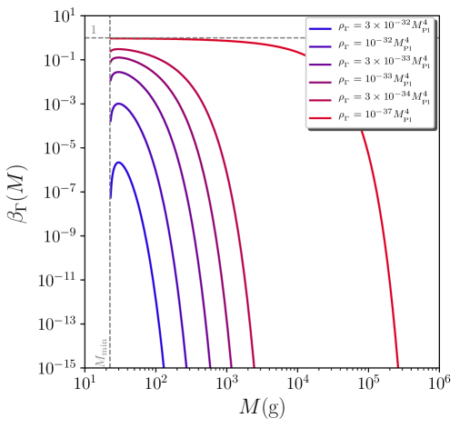
Figure 3: Mass fraction of PBHs at the end of the instability phase, as a function of the mass at which they form. The energy density at the end of inflation is set to $\rho_{\mathrm{inf}}=10^{-12}M_{\scriptscriptstyle{\mathrm{Pl}}}^{4}\simeq(2.43\times 10^{15}\mathrm{GeV})^{4}$, and the result is displayed for a few values of $\rho_{\Gamma}$, namely $\rho_{\Gamma}=3\times 10^{-32}M_{\scriptscriptstyle{\mathrm{Pl}}}^{4}\simeq(3.2\times 10^{10}\mathrm{GeV})^{4}$, $\rho_{\Gamma}=10^{-32}M_{\scriptscriptstyle{\mathrm{Pl}}}^{4}\simeq(2.4\times 10^{10}\mathrm{GeV})^{4}$, $\rho_{\Gamma}=3\times 10^{-33}M_{\scriptscriptstyle{\mathrm{Pl}}}^{4}\simeq(1.8\times 10^{10}\mathrm{GeV})^{4}$, $\rho_{\Gamma}=10^{-33}M_{\scriptscriptstyle{\mathrm{Pl}}}^{4}\simeq(1.4\times 10^{10}\mathrm{GeV})^{4}$, $\rho_{\Gamma}=3\times 10^{-34}M_{\scriptscriptstyle{\mathrm{Pl}}}^{4}\simeq(10^{10}\mathrm{GeV})^{4}$ and $\rho_{\Gamma}=10^{-37}M_{\scriptscriptstyle{\mathrm{Pl}}}^{4}\simeq(1.4\times 10^{9}\mathrm{GeV})^{4}$. The vertical grey dashed line stands for the minimum mass corresponding to the scale that matches the Hubble radius at the end of inflation, while the horizontal grey dashed line corresponds to $\beta=1$, which is the maximum possible value attained in the limit $\delta_{\mathrm{c}}\ll\mathchoice{{\hbox{$\displaystyle\sqrt{\mathcal{P}_{\delta}\,}$}\lower 0.4pt\hbox{\vrule height=6.83331pt,depth=-5.46667pt}}}{{\hbox{$\textstyle\sqrt{\mathcal{P}_{\delta}\,}$}\lower 0.4pt\hbox{\vrule height=6.83331pt,depth=-5.46667pt}}}{{\hbox{$\scriptstyle\sqrt{\mathcal{P}_{\delta}\,}$}\lower 0.4pt\hbox{\vrule height=4.78333pt,depth=-3.82668pt}}}{{\hbox{$\scriptscriptstyle\sqrt{\mathcal{P}_{\delta}\,}$}\lower 0.4pt\hbox{\vrule height=3.41666pt,depth=-2.73334pt}}}$.

The mass fraction at the end of the instability phase can be computed using the above relations, and is displayed as a function of the mass in Fig. 3, for $\rho_{\mathrm{inf}}=10^{-12}M_{\scriptscriptstyle{\mathrm{Pl}}}^{4}\simeq\left(2.43\times 10^{15}\mathrm{GeV}\right)^{4}$ and a few values of $\rho_{\Gamma}$. We also take $10240/g=100$ and $\xi=1$. The vertical grey dashed line stands for the minimum mass $M_{\mathrm{min}}$, corresponding to the scale that matches the Hubble radius at the end of inflation, and which can be obtained by setting $k/k_{\mathrm{end}}=1$ in Eq. (3.5). For the value of $\rho_{\mathrm{inf}}$ used in the figure, one has $M_{\mathrm{min}}\simeq 22.5\,\mbox{g}\simeq 1.1\times 10^{-32}M_{\odot}$, where $M_{\odot}$ denotes the mass of the sun. Since the result depends only on $\rho_{\mathrm{inf}}$, and given that the same value of $\rho_{\mathrm{inf}}$ is used for all curves, this explains why the same value for the minimum mass is found. One can also check that, the lower $\rho_{\Gamma}$ is, the longer the instability phase is, hence the more amplified the fluctuations are and the more black holes are produced.

The dependence of $\beta(M,t_{\Gamma})$ in terms of the mass $M$ can also be understood in simple terms. The dominant trend is that the mass fraction mostly decreases with the value of the mass. This is because, the larger the mass, the smaller the wavenumber $k$ [see Eq. (3.5)], hence the later the mode enters the instability band, so the less amplified the perturbation and the larger $\delta_{\mathrm{c}}$ [see Eq. (3.4)]. More precisely, for $\delta_{\mathrm{max}}=1$, from Eq. (3.8), $\beta$ decreases with $\delta_{\mathrm{c}}/\mathchoice{{\hbox{$\displaystyle\sqrt{2\mathcal{P}_{\delta}\,}$}\lower 0.4pt\hbox{\vrule height=6.83331pt,depth=-5.46667pt}}}{{\hbox{$\textstyle\sqrt{2\mathcal{P}_{\delta}\,}$}\lower 0.4pt\hbox{\vrule height=6.83331pt,depth=-5.46667pt}}}{{\hbox{$\scriptstyle\sqrt{2\mathcal{P}_{\delta}\,}$}\lower 0.4pt\hbox{\vrule height=4.78333pt,depth=-3.82668pt}}}{{\hbox{$\scriptscriptstyle\sqrt{2\mathcal{P}_{\delta}\,}$}\lower 0.4pt\hbox{\vrule height=3.41666pt,depth=-2.73334pt}}}$. Since $\delta_{\mathrm{c}}\propto k^{-2}$, see Eq. (3.4), $\beta$ decreases with $M$ (hence increases with $k$) if $\mathrm{d}\ln\mathcal{P}_{\zeta}/\mathrm{d}\ln k>-4$, i.e. if the spectral index is larger than $-3$. This is of course the case away from the end of inflation, where the power spectrum is close to scale invariance, but might not be true for modes that exit the Hubble radius close to the end of inflation, i.e. for values of $M$ close to $M_{\mathrm{min}}$. In fact, one can check that the spectral index corresponding to the “numerical” power spectrum in Fig. 1 (blue curve) is always larger than $-3$, and the reason why $\beta$ increases with $M$ at small masses in some of the curves displayed in Fig. 3 is because we make use of the slow-roll approximation (2.8) corresponding to the black dashed curve in Fig. 1, for which the spectral index drops below $-3$ at the very end of inflation. However, as stressed above, although this approximation is necessary to limit the numerical cost of the parameter space exploration performed below, it only affects a tiny range of modes that exit the Hubble radius at the very end of inflation, and is conservative in the sense of footnote 4.

3.4 Renormalising the mass fraction at the end of the instability

Figure 4: Mass fraction of PBHs at the end of the instability phase, as a function of the mass at which the black holes form, for $\rho_{\mathrm{inf}}=10^{-12}M_{\scriptscriptstyle{\mathrm{Pl}}}^{4}\simeq\left(2.43\times 10^{15}\mathrm{GeV}\right)^{4}$ and $\rho_{\Gamma}=10^{-40}M_{\scriptscriptstyle{\mathrm{Pl}}}^{4}\simeq\left(2.43\times 10^{8}\mathrm{GeV}\right)^{4}$. The black line corresponds to the result obtained before renormalisation and leads to $\Omega_{\mathrm{PBH}}(t_{\Gamma})=8.54>1$, which is not physical. The blue dotted line is obtained after renormalisation by inclusion, i.e. when increasing $M_{\mathrm{min}}$ to $M_{\mathrm{min}}^{\prime}$ such that the integrated mass fraction $\Omega_{\mathrm{PBH}}(t_{\Gamma})$ becomes one. This accounts for the absorption of small-black holes into larger-mass black holes when the regions that collapse into these large-mass black holes already contain smaller ones. The green dotted line stands for renormalisation by premature ending, i.e. by stopping the instability phase before $t_{\Gamma}$, at the time when $\Omega_{\mathrm{PBH}}$ reaches one. This accounts for the fact that if the universe becomes dominated by black holes, the parametric resonance effect stops.

The fraction of the energy density of the universe contained within PBHs at the end of the instability phase is, by definition, given by

$$\Omega_{\mathrm{PBH}}\left(t_{\Gamma}\right)=\int_{M_{\mathrm{min}}}^{M_{\mathrm{max}}}\beta\left(M,t_{\Gamma}\right)\mathrm{d}\ln M\,.$$ (3.11)

One can compute its value for the parameters displayed in Fig. 3 and one finds $\Omega_{\mathrm{PBH}}(t_{\Gamma})\simeq 8.68\times 10^{-7},\ 5.63\times 10^{-4},\ 2.13\times 10^{-2},\ 0.129,\ 0.412,\ 4.58$ for $\rho_{\Gamma}=3\times 10^{-32}M_{\scriptscriptstyle{\mathrm{Pl}}}^{3},\cdots,10^{-37}M_{\scriptscriptstyle{\mathrm{Pl}}}^{4}$, respectively. The fact that $\Omega_{\mathrm{PBH}}$ decreases with $\rho_{\Gamma}$ is consistent with what precedes, but the reader should be struck by the last value, which is above one. This is of course not possible given that we assume the spatial curvature to vanish, and entails that when $\rho_{\Gamma}$ decreases, the production of PBHs is so efficient that they overtake the energy density stored in the inflaton field. When this happens, the above approach breaks down. Below, we propose two procedures to model what may physically prevent $\Omega_{\mathrm{PBH}}$ to grow larger than one.

3.4.1 Renormalisation by inclusion

When $\Omega_{\mathrm{PBH}}$ increases and reaches sizeable values, PBHs are densely distributed in the universe, and when a fluctuation at a given scale gets amplified above the threshold, the region of space that collapses and forms a black hole may already contain smaller black holes. If this happens, when black holes with larger masses form, black holes with smaller masses may be absorbed and disappear from the mass fraction, and we dub this effect “inclusion”. In LABEL:MoradinezhadDizgah:2019wjf, this is also called the “could-in-cloud” phenomenon.

In that case, we proceed as follows: if $\Omega_{\mathrm{PBH}}(t_{\Gamma})$ is found to be larger than one, we increase the value of $M_{\mathrm{min}}$ in Eq. (3.11),

$$M_{\mathrm{min}}\rightarrow M_{\mathrm{min}}^{\prime}\,,$$ (3.12)

in such a way that $\Omega_{\mathrm{PBH}}(t_{\Gamma})$ becomes one. We therefore remove the small mass tail of the distribution that is responsible for having $\Omega_{\mathrm{PBH}}>1$, accounting for their absorption into larger-mass black holes.

One should note that this inclusion effect might, in practice, prevent $\Omega_{\mathrm{PBH}}$ to grow larger than some intermediate value that is smaller than one, but this would have only very little impact on the results derived below as long as that value is of order one (which is expected for the inclusion phenomenon to be significant [50]). Another possibility is that small-black holes are indeed removed from the distribution, but that the decrease in $\beta$ at small $M$ is smoother than a sharp cutoff imposed at $M_{\mathrm{min}}^{\prime}$. In the absence of a clear way to model the formation of PBHs and the inclusion dynamics in the dense regime, it seems difficult to go beyond the sharp cutoff procedure, which can however be seen as a limit bounding the range of possible renormalisation procedures (the other bounding procedure being introduced below).

In Fig. 4, we have represented the mass fraction at the end of the instability phase for $\rho_{\mathrm{inf}}=10^{-12}M_{\scriptscriptstyle{\mathrm{Pl}}}^{4}\simeq\left(2.43\times 10^{15}\mathrm{GeV}\right)^{4}$ and $\rho_{\Gamma}=10^{-40}M_{\scriptscriptstyle{\mathrm{Pl}}}^{4}\simeq\left(2.43\times 10^{8}\mathrm{GeV}\right)^{4}$. The black solid line corresponds to what is obtained before renormalisation and leads to $\Omega_{\mathrm{PBH}}(t_{\Gamma})=8.54$, which is not possible. The blue dotted line represents the result after renormalisation by inclusion (3.12), i.e. by removing the low mass part of the distribution to bring $\Omega_{\mathrm{PBH}}(t_{\Gamma})$ back to one.

3.4.2 Renormalisation by premature ending

Another possibility is that, as $\Omega_{\mathrm{PBH}}$ increases, PBHs backreact on the dynamics of the universe, which is no longer dominated by the coherent oscillations of the inflaton field, and the instability stops. The precise value of $\Omega_{\mathrm{PBH}}$ at which this premature termination occurs is difficult to assess, and for simplicity we will assume it to be one, since our final results mildly depend on it.

In that case, if $\Omega_{\mathrm{PBH}}(t_{\Gamma})$ is found to be larger than one, we change the time at which the instability stops,

$$t_{\Gamma}\rightarrow t_{\mathrm{instab}},$$ (3.13)

where $t_{\mathrm{instab}}$ is the time at which $\Omega_{\mathrm{PBH}}$ reaches one. Therefore, as announced before, there are situations for which $t_{\mathrm{instab}}\neq t_{\Gamma}$. The result is displayed in Fig. 4 with the dotted green line. One can check that the large-mass black holes are removed from the mass fraction distribution, since those black holes correspond to scales that enter the instability band towards the end of the instability phase, at which point the instability is now no longer on.

Since, as explained above, the procedure of renormalisation by inclusion removes the small-mass end of the distribution, these two approaches can therefore be viewed as complementary, and by studying the results obtained with both one can assess how much the conclusions depend on the way the mass fraction is renormalised.

The actual renormalisation procedure might lie in between these two schemes: for instance, it could happen that, as $\Omega_{\mathrm{PBH}}$ increases, inclusion starts to be important, which slows down the increase of $\Omega_{\mathrm{PBH}}$ but does not prevent it from further growing, until the point where premature ending occurs. In such a case, a distribution that is intermediate between the blue and the green curves of Fig. 4 would be obtained. As we will show below, some common conclusions can be drawn with both renormalisation schemes, which motivates the statement that such conclusions are mildly dependent on the renormalisation approach.

3.5 Evolving the mass fraction

Figure 5: Integrated mass fraction $\Omega_{\mathrm{PBH}}$ as a function of time, here parametrised by the total energy density $\rho_{\mathrm{tot}}$, from the end of the instability phase $t_{\mathrm{instab}}$ until BBN, for the same values of $\rho_{\mathrm{inf}}$ and $\rho_{\Gamma}$ as the ones displayed in Fig. 3. For $\rho_{\Gamma}=10^{-37}M_{\scriptscriptstyle{\mathrm{Pl}}}^{4}\simeq(1.4\times 10^{9}\mathrm{GeV})^{4}$, the mass fraction needs to be renormalised, which for illustration here is done using the premature-ending procedure.

After the instability stops, the density of black holes evolves under different physical effects, such as Hawking evaporation, accretion and merging. In what follows we neglect the two latter and only account for the former. The reason is that accretion and merging are technically difficult to model (see e.g. Refs. [51, 52]), and only contribute to enhancing the final value of $\Omega_{\mathrm{PBH}}$. The reason why this is the case for accretion is obvious, and for merging, this is because the Hawking evaporation time (3.6) cubicly depends on the mass. Therefore, when two black holes (say of the same mass) merge, they loose some fraction of their mass through the emission of gravitational waves, but their evaporation time is multiplied by $8$, allowing them to live much longer. As a consequence, by only considering Hawking evaporation, we again derive conservative bounds, which underestimate the density of black holes at the epochs where they are observationally constrained.

The mass of a black hole decreases under Hawking evaporation according to [48]

$$M(t,k)=M\left(t_{\mathrm{instab}},k\right)\left\{1-\frac{t-t_{\mathrm{instab}}}{\Delta t_{\mathrm{evap}}\left[M\left(t_{\mathrm{instab}},k\right)\right]}\right\}^{1/3}\,,$$ (3.14)

where $\Delta t_{\mathrm{evap}}$ was given in Eq. (3.6). This expression should be understood as coming with a Heaviside function such that, when $t-t_{\mathrm{instab}}>\Delta t_{\mathrm{evap}}$, $M$ is set to zero. We do not write it explicitly here for notational convenience. If $\bar{\beta}$ denotes the mass fraction in the absence of Hawking evaporation, one then has

$$\Omega_{\mathrm{PBH}}(t)=\int_{M_{\mathrm{min}}^{\prime}}^{M_{\mathrm{max}}}\bar{\beta}\left(M,t\right)\left[1-\frac{t-t_{\mathrm{instab}}}{\Delta t_{\mathrm{evap}}\left(M_{\mathrm{instab}}\right)}\right]^{1/3}\mathrm{d}\ln M\,,$$ (3.15)

where $M_{\mathrm{instab}}$ is a short-hand notation for $M(t_{\mathrm{instab}},k)$, and where one should recall that $M$ and $k$ are related through Eq. (3.5). Let us see how $\bar{\beta}$ can be calculated (in what follows, quantities with a bar denote their values in the absence of Hawking evaporation). The energy density of PBHs contained in an infinitesimal range of scales $\delta(\ln M)$ is given by $\delta\bar{\rho}=\rho_{\mathrm{tot}}\bar{\beta}\left(M,t\right)\delta(\ln M)$. Since PBHs behave as pressureless matter, in the absence of Hawking evaporation one would have $\dot{\delta\bar{\rho}}+3H\delta\bar{\rho}=0$. Plugging the former expression into the latter, one obtains $\left(\dot{\rho}_{\mathrm{tot}}+3H{\rho}_{\mathrm{tot}}\right)\bar{\beta}\left(M,t\right)+\rho_{\mathrm{tot}}\dot{\bar{\beta}}\left(M,t\right)=0$. After the end of the instability phase, we assume that the inflaton instantaneously decays into a radiation fluid, so $\bar{\rho}_{\mathrm{tot}}=\bar{\rho}_{\mathrm{PBH}}+\bar{\rho}_{\mathrm{rad}}$. In the absence of Hawking evaporation, one then has $\dot{\bar{\rho}}_{\mathrm{tot}}=-3H\bar{\rho}_{\mathrm{PBH}}-4H\bar{\rho}_{\mathrm{rad}}=-3H\Omega_{\mathrm{PBH}}\bar{\rho}_{\mathrm{tot}}-4H(1-\Omega_{\mathrm{PBH}})\bar{\rho}_{\mathrm{tot}}=H\bar{\rho}_{\mathrm{tot}}(\Omega_{\mathrm{PBH}}-4)$. This gives rise to

$$\dot{\bar{\beta}}(M,t)+H\left(\Omega_{\mathrm{PBH}}-1\right)\bar{\beta}(M,t)=0\,.$$ (3.16)

A priori, this equation has to be solved for each mass independently, with the corresponding initial condition at $t_{\mathrm{instab}}$. However, since the equation is linear and does not depend explicitly on the mass, a simpler solution to the problem can be found by introducing the function $\mathfrak{b}$ that satisfies

$$\dot{\mathfrak{b}}+H\left(\Omega_{\mathrm{PBH}}-1\right)\mathfrak{b}=0\quad\text{with}\quad\mathfrak{b}\left(t_{\mathrm{instab}}\right)=1\,,$$ (3.17)

and such that

$$\bar{\beta}\left(M,t\right)=\bar{\beta}\left(M,t_{\mathrm{instab}}\right)\mathfrak{b}\left(t\right)$$ (3.18)

satisfies Eq. (3.16), with the correct initial condition. The set of equations (3.15), (3.17) and (3.18) then defines a differential system that one can integrate numerically. Finally, let us note that, in practice, we would like to integrate the differential system until a time defined by its energy density rather than its cosmic time (for instance, until BBN defined by $\rho^{1/4}=\rho_{\mathrm{BBN}}^{1/4}\sim 10\,\mathrm{MeV}$). For this reason it is more convenient to use $\ln\rho_{\mathrm{tot}}$ as the time variable (the log being used for numerical convenience), and Eq. (3.17) becomes

$$\frac{\mathrm{d}\mathfrak{b}}{\mathrm{d}\ln\rho_{\mathrm{tot}}}+\frac{\Omega_{\mathrm{PBH}}-1}{\Omega_{\mathrm{PBH}}-4}\mathfrak{b}=0\,.$$ (3.19)

The value of cosmic time is still necessary in order to evaluate the Hawking suppression term in Eq. (3.15), which can be tracked solving

$$\frac{\mathrm{d}(t-t_{\mathrm{instab}})}{\mathrm{d}\ln\rho_{\mathrm{tot}}}=\frac{\mathchoice{{\hbox{$\displaystyle\sqrt{3\,}$}\lower 0.4pt\hbox{\vrule height=6.44444pt,depth=-5.15558pt}}}{{\hbox{$\textstyle\sqrt{3\,}$}\lower 0.4pt\hbox{\vrule height=6.44444pt,depth=-5.15558pt}}}{{\hbox{$\scriptstyle\sqrt{3\,}$}\lower 0.4pt\hbox{\vrule height=4.51111pt,depth=-3.6089pt}}}{{\hbox{$\scriptscriptstyle\sqrt{3\,}$}\lower 0.4pt\hbox{\vrule height=3.22221pt,depth=-2.57779pt}}}M_{\scriptscriptstyle{\mathrm{Pl}}}}{\left(\Omega_{\mathrm{PBH}}-4\right)\mathchoice{{\hbox{$\displaystyle\sqrt{\rho_{\mathrm{tot}}\,}$}\lower 0.4pt\hbox{\vrule height=4.30554pt,depth=-3.44446pt}}}{{\hbox{$\textstyle\sqrt{\rho_{\mathrm{tot}}\,}$}\lower 0.4pt\hbox{\vrule height=4.30554pt,depth=-3.44446pt}}}{{\hbox{$\scriptstyle\sqrt{\rho_{\mathrm{tot}}\,}$}\lower 0.4pt\hbox{\vrule height=3.01389pt,depth=-2.41113pt}}}{{\hbox{$\scriptscriptstyle\sqrt{\rho_{\mathrm{tot}}\,}$}\lower 0.4pt\hbox{\vrule height=2.15277pt,depth=-1.72223pt}}}}$$ (3.20)

together with the above system.

In Fig. 5, the solution one obtains for $\Omega_{\mathrm{PBH}}$ as a function of time is displayed for the same parameter values as the ones used in Fig. 3. At early time, the effect of Hawking evaporation is negligible, and $\rho_{\mathrm{PBH}}\propto a^{-3}$. If $\Omega_{\mathrm{PBH}}\ll 1$, $\rho_{\mathrm{tot}}\simeq\rho_{\mathrm{rad}}\propto a^{-4}$ and $\Omega_{\mathrm{PBH}}\propto a$, otherwise $\rho_{\mathrm{tot}}\simeq\rho_{\mathrm{PBH}}\propto a^{-3}$ and $\Omega_{\mathrm{PBH}}$ remains equal to one. Let us see when the black holes complete their evaporation. If a PBH forms from a scale that crosses in the instability band at $\rho_{\mathrm{bc}}$, its mass is given by setting $k/k_{\mathrm{end}}=(\rho_{\mathrm{bc}}/\rho_{\mathrm{inf}})^{1/6}$ in Eq. (3.5). Inserting the corresponding expression of $M$ into Eq. (3.6), the time $t_{\mathrm{evap}}-t_{\mathrm{instab}}$ at which it evaporates can be derived. If $\Omega_{\mathrm{PBH}}\ll 1$ until this point, Eq. (3.20) can be integrated and gives $\rho=\rho_{\mathrm{instab}}[1+2\mathchoice{{\hbox{$\displaystyle\sqrt{\rho_{\mathrm{instab}}/3\,}$}\lower 0.4pt\hbox{\vrule height=7.5pt,depth=-6.00003pt}}}{{\hbox{$\textstyle\sqrt{\rho_{\mathrm{instab}}/3\,}$}\lower 0.4pt\hbox{\vrule height=7.5pt,depth=-6.00003pt}}}{{\hbox{$\scriptstyle\sqrt{\rho_{\mathrm{instab}}/3\,}$}\lower 0.4pt\hbox{\vrule height=5.25pt,depth=-4.20003pt}}}{{\hbox{$\scriptscriptstyle\sqrt{\rho_{\mathrm{instab}}/3\,}$}\lower 0.4pt\hbox{\vrule height=3.75pt,depth=-3.00002pt}}}(t-t_{\mathrm{instab}})/M_{\scriptscriptstyle{\mathrm{Pl}}}]^{-2}$, which means that the black hole evaporates at the energy density

$$\rho_{\mathrm{evap}}\sim\frac{1}{26244\xi^{6}}\left(\frac{g}{10240}\right)^{2}\frac{\rho_{\mathrm{bc}}^{3}}{M_{\scriptscriptstyle{\mathrm{Pl}}}^{8}}\,.$$ (3.21)

Notice that, in order to obtain this estimate, we have neglected the fact that Hawking evaporation starts before the end of the instability (which was however taken into account for PBHs that entirely evaporate during the instability, see Sec. 3.2). Indeed, given than the collapsing time decays with the initial density contrast, see Eq. (3.1), and since PBHs form in the Gaussian tail of the distribution function where the smaller the density contrast, the more likely it is, most PBHs form close to the end of the instability phase, and for them Hawking evaporation during the instability can be neglected.

If $\Omega_{\mathrm{PBH}}$ takes sizeable values before the evaporation of the first black holes, the estimate (3.21) needs only to be corrected by factors of order one (If $\Omega_{\mathrm{PBH}}=1$, the corrective factor is $8/9$). The first black holes to evaporate are the ones with the smallest mass $M_{\mathrm{min}}$, i.e. such that $\rho_{\mathrm{bc}}=\rho_{\mathrm{inf}}$. In Fig. 5, one can check that the evaporation of these PBHs indeed corresponds to the turning point of all curves [for $\rho_{\mathrm{inf}}=10^{-12}M_{\scriptscriptstyle{\mathrm{Pl}}}^{4}\simeq\left(2.43\times 10^{15}\mathrm{GeV}\right)^{4}$, Eq. (3.21) gives $\rho_{\mathrm{evap}}\sim 3\times 10^{-45}M_{\scriptscriptstyle{\mathrm{Pl}}}^{4}\simeq\left(1.8\times 10^{7}\mathrm{GeV}\right)^{4}$]. Below this point, Hawking evaporation is efficient and $\Omega_{\mathrm{PBH}}$ quickly decreases.

3.6 Reheating through PBH evaporation

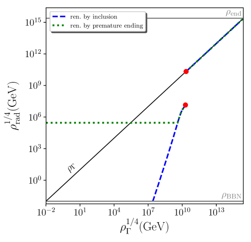
Figure 6: Energy density at the onset of the radiation era, $\rho_{\mathrm{rad}}$, as a function of $\rho_{\Gamma}$, for $\rho_{\mathrm{inf}}=10^{-12}M_{\scriptscriptstyle{\mathrm{Pl}}}^{4}\simeq\left(2.43\times 10^{15}\mathrm{GeV}\right)^{4}$ (which is the value used in all previous figures). The blue curve corresponds to the renormalisation procedure by inclusion, while the green one stands for renormalisation by premature ending. The red circles indicate the location of the discontinuity, i.e. values of $\rho_{\mathrm{rad}}$ comprised between the two circles are never realised, see main text.

The onset of the radiation era, defined as being the time, after the instability phase, after which $\Omega_{\mathrm{PBH}}$ remains below $1/2$, does not necessarily coincide with $t_{\mathrm{instab}}$. Indeed, if the universe is dominated by PBHs at the end of the instability, as is the case for the curve with $\rho_{\Gamma}=10^{-37}M_{\scriptscriptstyle{\mathrm{Pl}}}^{4}\simeq(1.4\times 10^{9}\mathrm{GeV})^{4}$ in Fig. 5, the radiation era only starts with the evaporation of the first black holes around $\rho\sim 10^{-45}M_{\scriptscriptstyle{\mathrm{Pl}}}^{4}\simeq(10^{7}\mathrm{GeV})^{4}$ as explained above. In fact, even if PBHs do not dominate the universe’s content at the end of the instability phase, they may later do so, see the curve with $\rho_{\Gamma}=3\times 10^{-33}M_{\scriptscriptstyle{\mathrm{Pl}}}^{4}\simeq(1.8\times 10^{10}\mathrm{GeV})^{4}$ in Fig. 5 for instance, in which case the onset of the radiation epoch is also delayed.

In such cases, let us point out that the reheating of the universe proceeds from the Hawking evaporation of the PBHs that dominate the energy budget for a transient period after the instability phase. If it completes long before BBN, such a mechanism is a priori allowed, and we discuss several of its implications in Sec. 5. It is then interesting to extract the energy density at the onset of the radiation period, $\rho_{\mathrm{rad}}$, from our computational pipeline. Let us notice that $\rho_{\mathrm{rad}}$ is the quantity which is related to what would be defined as the reheating temperature, $T_{\mathrm{reh}}$, through $\rho_{\mathrm{rad}}=g_{*}\pi^{2}T_{\mathrm{reh}}^{4}/30$, where $g_{*}$ is the number of relativistic degrees of freedom.

The quantity $\rho_{\mathrm{rad}}$ is displayed in Fig. 6 for $\rho_{\mathrm{inf}}=10^{-12}M_{\scriptscriptstyle{\mathrm{Pl}}}^{4}\simeq(2.43\times 10^{15}\mathrm{GeV})^{4}$ (which is the same value employed in all previous figures, in particular in Fig. 5) and as a function of $\rho_{\Gamma}$, which varies between $\rho_{\mathrm{BBN}}$ and $\rho_{\mathrm{inf}}$. This allows us to identify several relevant regions in parameter space. When $\rho_{\Gamma}$ is large, the instability phase is too short to produce a substantial amount of PBHs and they never dominate the energy content of the universe. This corresponds e.g. to the curve with $\rho_{\Gamma}=3\times 10^{-32}M_{\scriptscriptstyle{\mathrm{Pl}}}^{4}\simeq(3.2\times 10^{10}\mathrm{GeV})^{4}$ in Fig. 5. In this case, the radiation era starts when the inflaton decays into radiation, and $\rho_{\mathrm{rad}}=\rho_{\Gamma}$.

When $\rho_{\Gamma}$ decreases, one first notices in Fig. 6 the presence of a discontinuity, that we will explain shortly. In a small range below the discontinuity, $\rho_{\mathrm{rad}}$ is different from $\rho_{\Gamma}$, denoting the presence of a phase where PBHs dominate the universe, but does not depend on the renormalisation procedure, revealing that PBHs do not dominate at the end of the instability phase. This corresponds e.g. to the curve with $\rho_{\Gamma}=3\times 10^{-33}M_{\scriptscriptstyle{\mathrm{Pl}}}^{4}\simeq(1.8\times 10^{10}\mathrm{GeV})^{4}$ in Fig. 5. In this case, after the instability phase, there is a first radiation epoch, then PBHs take over and drive a matter epoch, before they evaporate and reheat the universe, which finally enters a second radiation epoch. One then finds $\rho_{\mathrm{rad}}<\rho_{\Gamma}$.

The discontinuity can be explained as follows: let us consider the case where radiation dominates at $t_{\Gamma}$, namely $\Omega_{\mathrm{PBH}}<1/2$ at $t_{\Gamma}$. Clearly, in this situation, no renormalisation is needed since $\Omega_{\mathrm{PBH}}<1$ at $t_{\Gamma}$. Then, as already explained, $\Omega_{\mathrm{PBH}}$ grows proportionally to the scale factor until Hawking evaporation becomes efficient and makes $\Omega_{\mathrm{PBH}}$ decrease, see Fig. 5. Assume that the maximum value $\Omega_{\mathrm{PBH}}$ reaches is slightly smaller than $1/2$. In this situation, the start of the radiation epoch is $t_{\Gamma}$ and $\rho_{\mathrm{rad}}=\rho_{\Gamma}$ since the radiation era is never interrupted. This case corresponds to the upper red dot in Fig. 6. Consider now the situation where at the end of the instability, the value of $\Omega_{\mathrm{PBH}}$ is infinitesimally larger than in the previous case (and, therefore, still smaller than $1/2$ at $t_{\Gamma}$). This means that we now start with a value of $\rho_{\Gamma}$ that is slightly smaller than before (and the instability lasts slightly longer). This gives rise to the same behaviour as described above except that, now, the value at the maximum is slightly larger than before, and above $1/2$. This means that the radiation epoch comes to an end and that a matter dominated era starts. Of course, since this is also the time at which Hawking radiation starts to become important, this matter-dominated era lasts a very short amount of time and very soon a new radiation dominated era (the “real” one) starts. The important point, however, is that $\rho_{\mathrm{rad}}$ is now very different from $\rho_{\Gamma}$ and is close to $\rho_{\mathrm{evap}}$, and this second case corresponds to the lower red dot in Fig. 6.

This explains the discontinuity in the curve $\rho_{\mathrm{rad}}$ versus $\rho_{\Gamma}$. Let us note that an important consequence of this behaviour is the fact that none of the values for $\rho_{\mathrm{rad}}$ comprised between the two red circles can be physically realised. We therefore identify regions in parameter space that are forbidden, not by the observations, but by self-consistency of the scenario itself.

Finally, when $\rho_{\Gamma}$ takes small values, PBHs are very abundantly produced and the mass fraction needs to be renormalised at the end of the instability phase. If renormalisation is carried out by inclusion, by keeping only the heavy black holes in the distribution, Hawking evaporation proceeds at later times when $\rho_{\Gamma}$ decreases, and the radiation epoch is more and more delayed. There is even a point where the radiation era has not started yet by BBN, which is obviously excluded and which explains why the blue curve is not plotted in Fig. 6 below that point. If renormalisation is performed by premature ending on the other hand, the result does not depend on $\rho_{\Gamma}$ since $\rho_{\mathrm{instab}}$ becomes independent of that parameter and, from there, the value of $\rho_{\mathrm{rad}}$ is only controlled by the evaporation process. In that case, for $\rho_{\Gamma}^{1/4}\gtrsim 286\mathrm{TeV}$, the onset of the radiation epoch is delayed compared to what it would have been if sourced by inflaton decay. This also implies that the inflaton could decay “inside” the black holes, although due to the no hair theorem, this should not leave any physical imprint. On the other hand, if $\rho_{\Gamma}^{1/4}\lesssim 286\mathrm{TeV}$, reheating occurs earlier than it would have with pure inflaton decay.

To conclude this section, let us stress again that, for $\rho_{\Gamma}\lesssim 10^{10}\mathrm{GeV}$ and $\rho_{\mathrm{inf}}=10^{-12}M_{\scriptscriptstyle{\mathrm{Pl}}}^{4}\simeq\left(2.43\times 10^{15}\mathrm{GeV}\right)^{4}$ (a full scan of the parameter space is presented in the following), namely below the lower red point in Fig. 6, the radiation in our universe no longer comes from inflaton decay but from the evaporation of PBHs formed during preheating. Given the generic character of the situation considered here (single-field inflation with quadratic minimum), this is clearly one of the main conclusions of the present paper.

3.7 Planckian relics

The previous considerations show that the universe may have gone through a phase where PBHs are numerous, and can even dominate the energy budget of the universe, but that these black holes can also well have all disappeared before BBN, through Hawking evaporation. In such a case, there is no direct way to constrain them, unless they do not fully evaporate and leave some relics behind.

This possibility has been discussed [57, 58] in the context of quantum-gravity inspired scenarios, where it has been suggested that black hole evaporation might stop when the mass of the black hole reaches the Planck mass. In this case, the number density of black hole can be computed at the end of the instability phase according to

$$n_{\mathrm{PBH}}\left(t_{\mathrm{instab}}\right)=\rho_{\mathrm{tot}}\int_{M_{\mathrm{min}}}^{M_{\mathrm{max}}}\frac{\tilde{\beta}\left(M,t_{\mathrm{instab}}\right)}{M}\mathrm{d}\ln M\,.$$ (3.22)

In this expression, $\tilde{\beta}\left(M,t_{\mathrm{instab}}\right)$ corresponds to Eq. (3.8) (with $t_{\Gamma}$ replaced with $t_{\mathrm{instab}}$) where, instead of taking $\delta_{\mathrm{max}}$ as being the minimum value between one and the right-hand side of Eq. (3.7), one simply takes $\delta_{\mathrm{max}}=1$. This ensures that the black holes that evaporate before the end of the instability phase are also accounted for in the calculation of relics.

Since this number density is not affected by Hawking evaporation, it then evolves according to the function $\mathfrak{b}(t)$ introduced in Sec. 3.5, i.e. solely under the effect of cosmic expansion. The fractional energy density of relics at subsequent times is thus given by

$$\Omega_{\mathrm{relics}}(t)=\mathfrak{b}(t)\int_{M_{\mathrm{min}}}^{M_{\mathrm{max}}}{\tilde{\beta}\left(M,t_{\mathrm{instab}}\right)}\frac{M_{\scriptscriptstyle{\mathrm{Pl}}}}{M}\mathrm{d}\ln M\,.$$ (3.23)

Let us note that this expression assigns one Planckian relic to each black hole, whether it has already evaporated or not. It therefore gives the density of “naked” relics only in the late-time limit, when all black holes have evaporated. It however always provides a lower bound on the contribution to dark matter (DM) originating from black holes and their relics, and as such, should be checked to be smaller than $\Omega_{\mathrm{DM}}$, which will be done in Sec. 4.3.

4 Observational consequences

Having described the physical setup and the methods employed to model it, let us now turn to the results and discuss their physical implications.

4.1 The onset of the radiation era

In Sec. 3.6, it was found that in some cases, the production of PBHs is so efficient that they may come to dominate the energy budget of the universe, either before the end of the instability phase or afterwards. In that case, the onset of the radiation era does not correspond to the time when the inflaton decays, i.e. when $\rho=\rho_{\Gamma}$, but rather occurs when the PBHs evaporate. The corresponding energy density, $\rho_{\mathrm{rad}}$, has been displayed as a function of $\rho_{\Gamma}$ and for a fixed value of $\rho_{\mathrm{inf}}$ in Fig. 6.

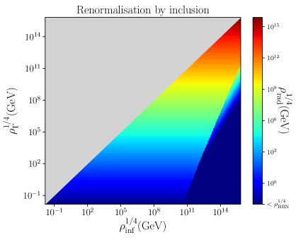
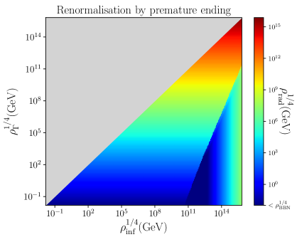
Figure 7: The energy density at the onset of the radiation era as a function of $\rho_{\mathrm{inf}}$ and $\rho_{\Gamma}$. The grey region is excluded since it corresponds to $\rho_{\mathrm{inf}}<\rho_{\Gamma}$. Left panel: renormalisation by inclusion. Right panel: renormalisation by premature ending.

In Fig. 7, the same quantity is shown, but as a function of both $\rho_{\mathrm{inf}}$ and $\rho_{\Gamma}$. Thus Fig. 6 is a vertical slice of Fig. 7. The left panel corresponds to renormalisation by inclusion, see Sec. 3.4.1, while the right panel stands for renormalisation by premature ending, see Sec. 3.4.2. The grey region is excluded since it corresponds to $\rho_{\Gamma}>\rho_{\mathrm{inf}}$. In the region where $\rho_{\mathrm{rad}}=\rho_{\Gamma}$, PBHs never dominate and reheating occurs at the end of the instability phase, through decay and thermalisation of the inflaton. In both figures, the lower right triangular regions, in which $\rho_{\mathrm{rad}}\neq\rho_{\Gamma}$, are such that reheating proceeds by PBH evaporation. Notice that, there, the darkest blue region corresponds to parameter values for which the universe is still not dominated by radiation at BBN, which is excluded. This allows us to generalise the remarks made around Fig. 6: when $\rho_{\Gamma}$ is large, the instability phase is short, PBHs never dominate the universe, so $\rho_{\mathrm{rad}}=\rho_{\Gamma}$ and reheating proceeds in the standard way; when $\rho_{\Gamma}$ is sufficiently small, PBHs can dominate the universe, which results into either delaying or anticipating the universe reheating. For $\rho_{\mathrm{inf}}^{1/4}\simeq 10^{15}\mathrm{GeV}$, which corresponds to a tensor-to-scalar ratio of $r\simeq 10^{-3}$, reheating occurs from PBHs evaporation when $\rho_{\Gamma}^{1/4}\lesssim 2\times 10^{9}\mathrm{GeV}$.

More generally, the boundary of the lower-right triangles, i.e. the condition for reheating the universe via PBH evaporation, can be worked out as follows. Clearly, reheating proceeds through PBHs evaporation if the PBHs are formed in a substantial way. This is the case if the critical density contrast given in Eq. (3.4), $\delta_{\mathrm{c}}\sim({3\pi}/{2})^{2/3}({k}/{k_{\mathrm{end}}})^{-2}({\rho_{\mathrm{inf}}}/{\rho_{\mathrm{instab}}})^{-1/3}=({3\pi}/{2})^{2/3}(\rho_{\mathrm{instab}}/\rho_{\mathrm{bc}})^{1/3}$ [where we have used $k/k_{\mathrm{end}}=(\rho_{\mathrm{bc}}/\rho_{\mathrm{inf}})^{1/6}$] is much smaller than $\textstyle\sqrt{2\mathcal{P}_{\delta}\,}$ . Moreover, the modes that get the more amplified are the ones that enter the instability band the earlier, and thus exit the Hubble radius not long before the end of inflation. For them, one can take $\mathcal{P}_{\zeta,\mathrm{end}}\sim H_{\mathrm{end}}^{2}/(8\pi^{2}M_{\scriptscriptstyle{\mathrm{Pl}}}^{2})$, see Eq. (2.8), hence $\mathcal{P}_{\delta,\mathrm{bc}}\sim 3\rho_{\mathrm{inf}}/(50\pi^{2}M_{\scriptscriptstyle{\mathrm{Pl}}}^{4})$, see Eq. (3.10). As a consequence, the condition $\delta_{\mathrm{c}}/\mathchoice{{\hbox{$\displaystyle\sqrt{2\mathcal{P}_{\delta}\,}$}\lower 0.4pt\hbox{\vrule height=6.83331pt,depth=-5.46667pt}}}{{\hbox{$\textstyle\sqrt{2\mathcal{P}_{\delta}\,}$}\lower 0.4pt\hbox{\vrule height=6.83331pt,depth=-5.46667pt}}}{{\hbox{$\scriptstyle\sqrt{2\mathcal{P}_{\delta}\,}$}\lower 0.4pt\hbox{\vrule height=4.78333pt,depth=-3.82668pt}}}{{\hbox{$\scriptscriptstyle\sqrt{2\mathcal{P}_{\delta}\,}$}\lower 0.4pt\hbox{\vrule height=3.41666pt,depth=-2.73334pt}}}\ll 1$ leads an upper bound on $\rho_{\mathrm{instab}}$, namely $\rho_{\mathrm{instab}}<4(125\mathchoice{{\hbox{$\displaystyle\sqrt{3\,}$}\lower 0.4pt\hbox{\vrule height=6.44444pt,depth=-5.15558pt}}}{{\hbox{$\textstyle\sqrt{3\,}$}\lower 0.4pt\hbox{\vrule height=6.44444pt,depth=-5.15558pt}}}{{\hbox{$\scriptstyle\sqrt{3\,}$}\lower 0.4pt\hbox{\vrule height=4.51111pt,depth=-3.6089pt}}}{{\hbox{$\scriptscriptstyle\sqrt{3\,}$}\lower 0.4pt\hbox{\vrule height=3.22221pt,depth=-2.57779pt}}}\pi^{5})^{-1}(\rho_{\mathrm{inf}}/M_{\scriptscriptstyle{\mathrm{Pl}}}^{4})^{3/2}\rho_{\mathrm{bc}}$. This makes sense since, in order to have sizeable PBHs production, the instability must last long enough and, therefore, $\rho_{\mathrm{instab}}$ must be small enough. Since $\rho_{\mathrm{bc}}<\rho_{\mathrm{inf}}$ and $\rho_{\Gamma}<\rho_{\mathrm{instab}}$ by construction, this gives rise to

$$\frac{\rho_{\Gamma}}{M_{\scriptscriptstyle{\mathrm{Pl}}}^{4}}<\frac{4}{125\mathchoice{{\hbox{$\displaystyle\sqrt{3\,}$}\lower 0.4pt\hbox{\vrule height=6.44444pt,depth=-5.15558pt}}}{{\hbox{$\textstyle\sqrt{3\,}$}\lower 0.4pt\hbox{\vrule height=6.44444pt,depth=-5.15558pt}}}{{\hbox{$\scriptstyle\sqrt{3\,}$}\lower 0.4pt\hbox{\vrule height=4.51111pt,depth=-3.6089pt}}}{{\hbox{$\scriptscriptstyle\sqrt{3\,}$}\lower 0.4pt\hbox{\vrule height=3.22221pt,depth=-2.57779pt}}}\pi^{5}}\left(\frac{\rho_{\mathrm{inf}}}{M_{\scriptscriptstyle{\mathrm{Pl}}}^{4}}\right)^{5/2}\,.$$ (4.1)

One can check that this expression provides a good fit to the boundary of the lower right triangular regions in Fig. 7, hence it gives a simple criterion to check whether or not reheating proceeds via PBH evaporation.

4.2 Constraints from the abundance of PBHs

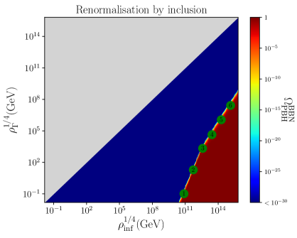
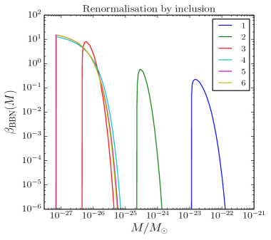
Figure 8: In the left panel, the fraction of the universe made of PBHs at BBN is displayed as a function of $\rho_{\mathrm{inf}}$ and $\rho_{\Gamma}$, when the mass fraction is renormalised by inclusion. The grey region corresponds to $\rho_{\Gamma}>\rho_{\mathrm{inf}}$ and is therefore forbidden. In the blue region, $\Omega_{\mathrm{PBH}}^{\mathrm{BBN}}<10^{-30}$, which leaves the parameters unconstrained. In the dark red region, $\Omega_{\mathrm{PBH}}^{\mathrm{BBN}}\simeq 1$, which is excluded. In between, there is a fine-tuned region where $\Omega_{\mathrm{PBH}}^{\mathrm{BBN}}$ takes fractional values, and where the details of the mass fraction matter. For that reason, $6$ points are labeled across that region, for which $\Omega_{\mathrm{PBH}}^{\mathrm{BBN}}=10^{-2}$, and their mass fraction is shown in the right panel.

Let us now discuss observational constraints from the predicted abundance of PBHs. The amount of DM made of PBHs is constrained by various astrophysical and cosmological probes, through their evaporation or gravitational effects (for a recent review, see e.g. LABEL:Carr:2009jm,_Carr:2017jsz). The earliest constraint, i.e. the one limiting black holes with the smallest mass, is BBN. This is why in the left panels of Figs. 8 and 9, the fraction of the universe made of PBHs at BBN is displayed, as a function of $\rho_{\mathrm{inf}}$ and $\rho_{\Gamma}$.

As before, the model is defined only when $\rho_{\Gamma}<\rho_{\mathrm{inf}}$, i.e. outside the grey region. The parameter space is otherwise essentially divided into two main regions: in the dark blue region, i.e. for large values of $\rho_{\Gamma}$, $\Omega_{\mathrm{PBH}}^{\mathrm{BBN}}\lesssim 10^{-30}$, and all observational constraints are easily passed. This corresponds to situations where PBHs are either not substantially produced, or evaporate before BBN. In the dark red region, i.e. for smaller values of $\rho_{\Gamma}$, $\Omega_{\mathrm{PBH}}^{\mathrm{BBN}}\simeq 1$ and the universe is not radiation dominated at the time of BBN, which is not allowed at more than the few percents level [59]. A substantial fraction of the reheating parameter space can therefore be excluded from the considerations presented in this work, which is our second main result. For instance, for the typical value $\rho_{\mathrm{inf}}^{1/4}\simeq 10^{15}\mathrm{GeV}$, $\Omega_{\mathrm{PBH}}^{\mathrm{BBN}}\gtrsim 0.1$ if $\rho_{\Gamma}^{1/4}\lesssim 1.6\times 10^{7}\mathrm{GeV}$ when renormalisation is performed by inclusion.

The location of the boundary between the excluded and the allowed regions can be worked out as follows. Requiring that the evaporation time, estimated in Eq. (3.21), is later than BBN leads to $\rho_{\mathrm{bc}}/M_{\scriptscriptstyle{\mathrm{Pl}}}^{4}<(9\times 6^{2/3})\xi^{2}(10240/g)^{2/3}(\rho_{\mathrm{BBN}}/M_{\scriptscriptstyle{\mathrm{Pl}}}^{4})^{1/3}$. In addition, we must also make sure that the corresponding PBHs have been produced in a non-negligible quantity which leads to the upper bound on $\rho_{\mathrm{instab}}$ derived in the text above Eq. (4.1). Combining these two expressions, one obtains $\rho_{\mathrm{instab}}/M_{\scriptscriptstyle{\mathrm{Pl}}}^{4}<(36\times 6^{2/3}\xi^{2})/(125\mathchoice{{\hbox{$\displaystyle\sqrt{3\,}$}\lower 0.4pt\hbox{\vrule height=6.44444pt,depth=-5.15558pt}}}{{\hbox{$\textstyle\sqrt{3\,}$}\lower 0.4pt\hbox{\vrule height=6.44444pt,depth=-5.15558pt}}}{{\hbox{$\scriptstyle\sqrt{3\,}$}\lower 0.4pt\hbox{\vrule height=4.51111pt,depth=-3.6089pt}}}{{\hbox{$\scriptscriptstyle\sqrt{3\,}$}\lower 0.4pt\hbox{\vrule height=3.22221pt,depth=-2.57779pt}}}\pi^{5})({10240}/{g})^{2/3}({\rho_{\mathrm{BBN}}}/{M_{\scriptscriptstyle{\mathrm{Pl}}}^{4}})^{1/3}({\rho_{\mathrm{inf}}}/{M_{\scriptscriptstyle{\mathrm{Pl}}}^{4}})^{3/2}\sim 2.5\times 10^{-29}({\rho_{\mathrm{inf}}}/{M_{\scriptscriptstyle{\mathrm{Pl}}}^{4}})^{3/2}$. Combined with Eq. (4.1), this gives rise to

$$\frac{\rho_{\mathrm{{instab}}}}{M_{\scriptscriptstyle{\mathrm{Pl}}}^{4}}<\mathrm{min}\left[6.0\times 10^{-5}\left(\frac{\rho_{\mathrm{inf}}}{M_{\scriptscriptstyle{\mathrm{Pl}}}^{4}}\right)^{5/2},\,2.5\times 10^{-29}\left(\frac{\rho_{\mathrm{inf}}}{M_{\scriptscriptstyle{\mathrm{Pl}}}^{4}}\right)^{3/2}\right]\,.$$ (4.2)

One can check that this rough estimate indeed provides a good enough description of the boundary between the blue and the red regions in Fig. 8 where one simply has $\rho_{\mathrm{instab}}=\rho_{\Gamma}$ (the situation in Fig. 9 is more complicated since those are two different quantities).

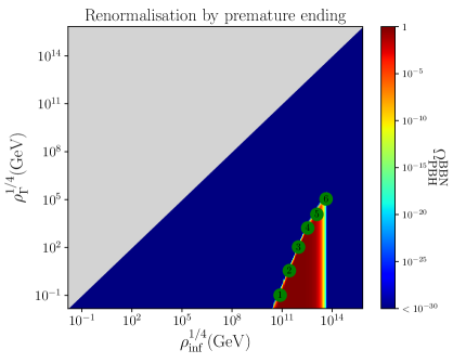
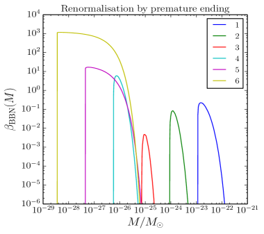
Figure 9: Same as in Fig. 8, when the mass fraction is renormalised by premature ending.

In between the excluded and the allowed regions, there is a fine-tuned, thin line along which $\Omega_{\mathrm{PBH}}^{\mathrm{BBN}}$ can take fractional values. There, the details of the mass fraction, i.e. the value of $\beta$ and the range of masses it covers, matter. For this reason, both in Figs. 8 and 9, we have sampled $6$ points along this thin line, for which $\Omega_{\mathrm{PBH}}^{\mathrm{BBN}}=10^{-2}$, and we show the corresponding mass fraction in the right panels, as a function of $M/M_{\odot}$. We have checked that fixing $\Omega_{\mathrm{PBH}}^{\mathrm{BBN}}$ to values different than $10^{-2}$ does not qualitatively change the following remarks.

First, one may be surprised that some values of $\beta$ are larger than one. This is because, although $\beta$ at the end of the instability is smaller than one by definition, see Eq. (3.8), it is then redshifted by $\mathfrak{b}$, see Eq. (3.18), which can be much larger than one. The integrated mass fraction, $\Omega_{\mathrm{PBH}}$, does always remain smaller than one.

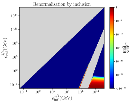
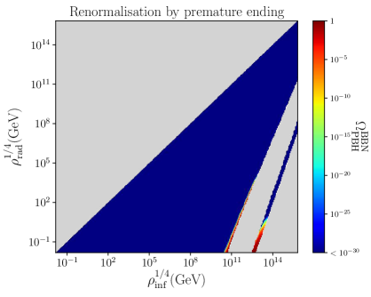
Figure 10: Fraction of the universe made of PBHs at BBN, as a function of $\rho_{\mathrm{inf}}$ and $\rho_{\mathrm{rad}}$, when the mass fraction is renormalised by inclusion (left panel) and premature ending (right panel). The grey region is not realised either because $\rho_{\mathrm{rad}}>\rho_{\mathrm{inf}}$, or because the corresponding value of $\rho_{\mathrm{rad}}$ is never realised, see the discussion around Fig. 6.

Second, the observational constraints on the value of $\beta$ depend on whether the mass distribution is monochromatic (i.e. all black holes have the same mass) or extended. In our case, it is clearly extended, and the constraints then depend on its precise profile. Let us however note [29] that the smallest mass being constrained is of the order $10^{-24}M_{\odot}$. Only the points labeled $1$ and $2$ in Figs. 8 and 9, i.e. the ones with $\rho_{\mathrm{inf}}\sim 10^{-30}M_{\scriptscriptstyle{\mathrm{Pl}}}^{4}\simeq(7.7\times 10^{10}\mathrm{GeV})^{4}$ and very small values of $\rho_{\Gamma}$, can therefore be constrained. More precisely, for monochromatic mass distributions, one has $\beta_{\mathrm{BBN}}(10^{-24}M_{\odot}<M<10^{-23}M_{\odot})<10^{-7}$ and $\beta_{\mathrm{BBN}}(10^{-23}M_{\odot}<M<10^{-19}M_{\odot})<10^{-12}$. Although this would have to be adapted to the extended mass distributions we are dealing with, this confirms that the points labeled $1$ and $2$ are probably excluded. This however does not change the main shape of the excluded region.

Third, no black hole with masses larger than $10^{-20}M_{\odot}$ are produced unless they are too abundantly produced. This implies that the present scenario cannot account for merger progenitors as currently seen in gravitational-wave detectors such as LIGO/VIRGO, nor can it explain dark matter since such black holes have all evaporated by now.

In Fig. 10, we finally display $\Omega_{\mathrm{PBH}}$ at BBN as a function of $\rho_{\mathrm{inf}}$ and $\rho_{\mathrm{rad}}$, in order to derive constraints in that parameter space too. As above, the upper-left grey triangle corresponds to $\rho_{\mathrm{rad}}>\rho_{\mathrm{inf}}$ and is therefore to be discarded. There are however additional grey regions corresponding to values of $\rho_{\mathrm{rad}}$ that are not realised: an intermediate grey band that stands for the discontinuity gap commented on around Fig. 6, and in the case of renormalisation by premature ending, a lower right grey triangle that arises from the saturation effect discussed around Fig. 6 as well.

4.3 Constraints from the abundance of Planckian relics

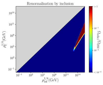
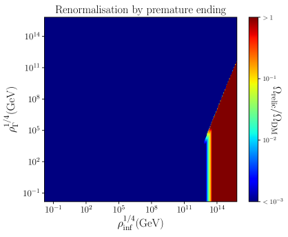
Figure 11: Abundance of Planckian relics normalised to the one of dark matter, as a function of $\rho_{\mathrm{inf}}$ and $\rho_{\Gamma}$, when the mass fraction is renormalised by inclusion (left panel) and premature ending (right panel).

In Sec. 3.7, we discussed the possibility that evaporated PBHs leave Planckian relics behind, i.e. objects of mass $\sim M_{\scriptscriptstyle{\mathrm{Pl}}}$ that do not further evaporate. If they exist, their density is expressed in Eq. (3.23), and it should be smaller than the one of dark matter. This is why in Fig. 11, the ratio $\Omega_{\mathrm{relic}}/\Omega_{\mathrm{DM}}$ is displayed, as a function of $\rho_{\mathrm{inf}}$ and $\rho_{\Gamma}$, and in Fig. 12, as a function $\rho_{\mathrm{inf}}$ and $\rho_{\mathrm{rad}}$. Similarly to Fig. 10, one can see that parameter space is essentially divided into two regions: one (dark blue) where the amount of Planckian relics left over from PBHs is negligible, and one (dark red) that is excluded since Planckian relics overtake the dark matter abundance. From Fig. 11, we see that, if $\rho_{\mathrm{inf}}^{1/4}\simeq 10^{15}\mathrm{GeV}$, then $\Omega_{\mathrm{relics}}>\Omega_{\mathrm{DM}}$ if $4.1\times 10^{7}\mathrm{GeV}\lesssim\rho_{\Gamma}^{1/4}\lesssim 4.0\times 10^{9}\mathrm{GeV}$ and renormalisation is performed by inclusion. If it is performed by premature ending, then $\Omega_{\mathrm{relics}}>\Omega_{\mathrm{DM}}$ if $\rho_{\Gamma}^{1/4}\lesssim 4.0\times 10^{9}\mathrm{GeV}$. Further regions of parameter space can thus be excluded from the predicted abundance of relics, if they exist. In between the excluded and allowed regions, there is a fine-tuned boundary where Planckian relics could constitute a substantial fraction of the dark matter.

5 Discussion and conclusions

In this work, we have shown how the coherent oscillations of the inflaton field around a local minimum of its potential at the end of inflation can lead to the resonant amplification of its fluctuations at small scales, that can then collapse and form PBHs. We have shown how the abundance and mass distribution of these PBHs can be calculated from the spectrum of fluctuations as predicted by inflation. In some cases, it was found that the production mechanism is so efficient that one needs to account for possible inclusion effects, and/or for the possibility that PBHs backreact and prematurely terminate the preheating instability. In such cases, the universe undergoes a phase where it is dominated by a gas of PBHs, that later reheats the universe by Hawking evaporation. This happens when Eq. (4.1) is satisfied.

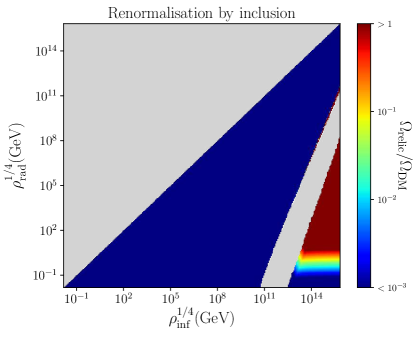
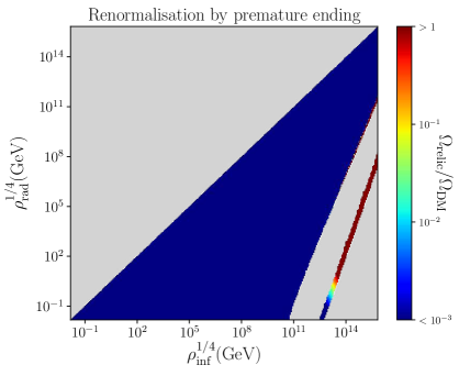
Figure 12: Abundance of Planckian relics normalised to the one of dark matter, as a function of $\rho_{\mathrm{inf}}$ and $\rho_{\mathrm{rad}}$, when the mass fraction is renormalised by inclusion (left panel) and premature ending (right panel).

A first result obtained in the present paper is therefore that, in the most simple models of inflation, reheating does not necessarily occur via inflaton decay, but for a large fraction of parameter space, it rather proceeds from the evaporation of PBHs produced during preheating. For the iconic value $\rho_{\mathrm{inf}}^{1/4}\simeq 10^{15}\mathrm{GeV}$ (corresponding to a tensor-to-scalar ratio $r\sim 10^{-3}$), this is the case provided $\rho_{\Gamma}^{1/4}\lesssim 2\times 10^{9}\mathrm{GeV}$. This deeply modifies our view of how the universe is reheated in the context of the inflationary theory: the radiation in our universe could well originate from Hawking radiation rather than from inflaton decay as usually thought.

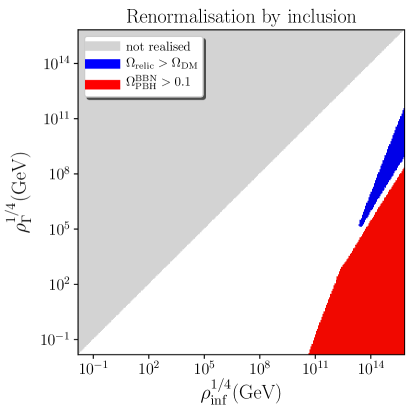
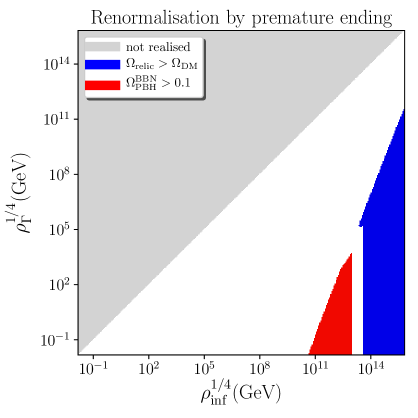
Figure 13: Combined constraints in the the space $(\rho_{\mathrm{inf}},\rho_{\Gamma})$, when the mass fraction is renormalised by inclusion (left panel) and premature ending (right panel). Red regions are excluded since they yield a too large abundance of primordial black holes. If black holes leave Planckian relics behind after evaporation, the blue regions are also excluded since they lead to too many of them. The remaining region, displayed in white, is the allowed one.

A second result concerns the constraints on the energy scale of inflation and the energy at the onset of the radiation-dominated epoch that follow from the above-described mechanism. These combined constraints on the two parameters describing our setup, either $\rho_{\mathrm{inf}}$ and $\rho_{\Gamma}$ or $\rho_{\mathrm{inf}}$ and $\rho_{\mathrm{rad}}$, are given in Fig. 13 and Fig. 14 respectively. All coloured regions are excluded: the grey one since it corresponds to values of $\rho_{\Gamma}$ and/or $\rho_{\mathrm{rad}}$ that cannot be realised; the red one since it leads to an overproduction of PBHs that is excluded by observations; and, if evaporated black holes leave Planckian relics behind, the blue one since it yields more relics than the measured abundance of dark matter. Only the white region remains, which strongly constrains the energy scale of inflation and reheating. For $\rho_{\mathrm{inf}}^{1/4}\simeq 10^{15}\mathrm{GeV}$, if renormalisation is performed by inclusion, values such that $\rho_{\Gamma}^{1/4}\lesssim 2\times 10^{9}\mathrm{GeV}$ and $4.1\times 10^{7}\mathrm{GeV}\lesssim\rho_{\Gamma}^{1/4}\lesssim 4.0\times 10^{9}\mathrm{GeV}$ are excluded. If renormalisation is performed by premature ending, then values such that $\rho_{\Gamma}^{1/4}\lesssim 4.0\times 10^{9}\mathrm{GeV}$ are excluded. The constraints on $\rho_{\mathrm{rad}}$ are also relevant since, as already mentioned, they correspond to constraints on the reheating temperature. For $\rho_{\mathrm{inf}}^{1/4}\simeq 10^{15}\mathrm{GeV}$, if renormalisation is performed by inclusion, we find that only values such that $10^{2}\mathrm{MeV}\lesssim\rho_{\mathrm{rad}}^{1/4}\lesssim 6\mathrm{GeV}$ and $\rho_{\mathrm{rad}}^{1/4}\gtrsim 4\times 10^{9}\mathrm{GeV}$ are allowed. If renormalisation is performed by premature ending, then only $\rho_{\mathrm{rad}}^{1/4}\gtrsim 4\times 10^{9}\mathrm{GeV}$ is possible.

This has very important implications. For instance, the Starobinsky model and the Higgs inflation models, which are among the best models of inflation [16, 17] and yield a tensor-to-scalar ratio of $r\simeq 10^{-3}$, share the same potential but have different reheating temperatures. More precisely, the Starobinsky model is usually associated with low reheating temperatures (typically $T_{\mathrm{reh}}\sim 10^{8}\mathrm{GeV}$ in supergravity embeddings, see LABEL:Terada:2014uia), and Higgs inflation with large reheating temperatures such as $T_{\mathrm{reh}}\simeq 10^{12}\mathrm{GeV}$ [61, 62, 63], see e.g. Fig. 2 in LABEL:Martin:2016iqo. Using $\rho_{\mathrm{rad}}^{1/4}\simeq(\pi^{2}g_{*}/30)^{1/4}T_{\mathrm{reh}}$ with $g_{*}\simeq 1000$, this leads to $\rho_{\mathrm{rad}}^{1/4}\simeq 4.2\times 10^{8}\mathrm{GeV}$ for the Starobinsky model and $\rho_{\mathrm{rad}}^{1/4}\simeq 4.2\times 10^{12}\mathrm{GeV}$ for Higgs inflation. According to the constraints obtained here, the reheating temperatures typically associated with the Starobinsky model are therefore excluded.

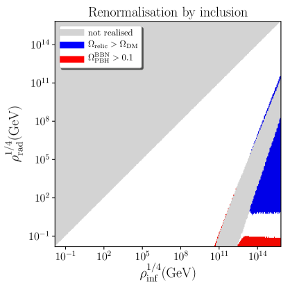
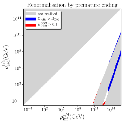
Figure 14: Combined constraints in the the space $(\rho_{\mathrm{inf}},\rho_{\mathrm{rad}})$, when the mass fraction is renormalised by inclusion (left panel) and premature ending (right panel). The grey regions are excluded since they correspond to values of $\rho_{\mathrm{rad}}$, the energy density at the onset of the radiation epoch, that cannot be realised. Red regions are excluded since they yield too large abundance of primordial black holes. If black holes leave Planckian relics behind after evaporation, the blue regions are also excluded since they lead to too many of them. The remaining region, displayed in white, is the one allowed.

Finally, let us comment on the robustness of our results. One should note that in the case where PBHs are abundantly produced, the use of the Press-Schechter formalism, or of the peak theory, might be questionable since those typically assume PBHs to be rare events. The precise way in which the mass fraction needs to be renormalised is also an open question in that case. By considering two extreme possibilities, i.e. black hole inclusion and premature ending of the instability, we have tried to cover the range of the possible outcomes from that renormalisation procedure, but it would be clearly more satisfactory to have a better description of PBHs production in the dense regime.

Let us also stress that over the course of the present analysis, conservative assumptions have been made, which tend to underestimate the predicted abundance of PBHs, in order to make safe the statement that the coloured regions in Figs. 13 and 14 are excluded. It would however be interesting to go beyond these assumptions and make the constraints even tighter.

Another effect we have neglected is black-hole accretion and merging. Since the evaporation time of PBHs scales as their masses cubed, see Eq. (3.6), accretion and merging make them live longer and modelling these effects would therefore render our bounds tighter. This might be of little importance when the abundance of PBHs is tiny, but it may play a bigger role in the case where PBHs transiently dominate the universe content. In that case, one may also expect that substantial amounts of gravitational waves are emitted by PBH mergers, which provides another channel through which the preheating instability could be constrained.

Let us also mention that in the analysis of Appendixes A and B, for simplicity, the over-density has been assumed to be initially spherically symmetric. The impact of deviations from spherically symmetric configurations on the production of PBHs has been studied in dust-like environment, e.g. in LABEL:Harada:2016mhb, where it has been shown that it can play an important role, and substantially decrease the abundance of the black holes. One may expect similar effects for black holes forming from a massive scalar field inhomogeneity [66, 45], although the situation is different and techniques developed to track perfect fluid inhomegeneities cannot be directly applied here. One would thus have to generalise the analysis of Appendixes A and B to non-spherically symmetric configurations, which may require a numerical approach and which we leave for future work. This may lead to less black holes than what we have estimated in the present work, although it is worth mentioning that non-spherically symmetric configurations should also provide spins to the resulting black holes. Since the Hawking evaporation time depends on the spin [68], PBHs forming from non-spherically symmetric over-densities have different life times, and are affected by observational constraints differently.

It is also worth stressing that the preheating instability has here been discussed in the context of a quadratic potential, since most inflationary potentials are quadratic close to their minimum, but it also takes place for quartic potentials [24]. In that case, the instability is even more pronounced, but it is restricted to a narrower range of modes, and it would be interesting to study its consequences for PBH formation.

Finally, let us mention that CMB predictions are also affected by our results. As explained in Sec. 1, for a fixed inflationary single-field potential, the only theoretical uncertainty in observational predictions is on the number of e-folds elapsed between the time when the CMB pivot scale exits the Hubble radius and the end of inflation. This number depends [14] on the energy scale of inflation, which is given by the inflationary model under consideration, the energy density at which the radiation era starts, and the averaged equation-of-state parameter between the end of inflation and that time. By restricting these values, the present work allows one to make inflationary predictions more focused, and this will be the topic of a separate article.

Appendix A Black holes formation from scalar field collapse

In this first appendix, we review (and correct a few typos in the work of) LABEL:Goncalves:2000nz, that studies black hole formation from massive scalar field collapse. Let us consider an inhomogeneous massive scalar field $\phi(t,r)$ living in an inhomogeneous but isotropic (spherically symmetric) space time endowed with the metric

$$\mathrm{d}s^{2}=-\mathrm{d}t^{2}+e^{-2\Lambda(t,r)}\mathrm{d}r^{2}+R^{2}(t,r)\left(\mathrm{d}\theta^{2}+\sin^{2}\theta\mathrm{d}\varphi^{2}\right).$$ (A.1)

In order to follow the evolution of the scalar field, we must solve the corresponding Einstein equations $G_{\mu\nu}=T_{\mu\nu}/M_{\scriptscriptstyle{\mathrm{Pl}}}^{2}$ where $T_{\mu\nu}=\partial_{\mu}\phi\partial_{\nu}\phi-\frac{1}{2}g_{\mu\nu}\left(g^{\alpha\beta}\partial_{\alpha}\phi\partial_{\beta}\phi+m_{\phi}^{2}\phi^{2}\right)$ is the stress energy tensor of the scalar field ($m_{\phi}$ is the mass of the field) and the Klein-Gordon equation $\left(g^{\mu\nu}\nabla_{\mu}\nabla_{\nu}-m^{2}_{\phi}\right)\phi=0$. This last equation takes the following form

$$\ddot{\phi}-e^{2\Lambda}\phi^{\prime\prime}+\left(2\frac{\dot{R}}{R}-\dot{\Lambda}\right)\dot{\phi}-e^{2\Lambda}\left(2\frac{R^{\prime}}{R}+\Lambda^{\prime}\right)\phi^{\prime}+m_{\phi}^{2}\phi=0,$$ (A.2)

where a dot denotes a derivative with respect to time and a prime a derivative with respect to the radial coordinate $r$. This Klein-Gordon equation should be compared to Eq. (7) of LABEL:Goncalves:2000nz. The two formula are nearly identical but there are sign differences. As can be seen on the above expression, in Eq. (7) of LABEL:Goncalves:2000nz, $2\dot{R}/R+\dot{\Lambda}$ should read $2\dot{R}/R-\dot{\Lambda}$ and $-2R^{\prime}/R+\Lambda^{\prime}$ should read $2R^{\prime}/R+\Lambda^{\prime}$.

Then, the components of the Einstein tensor are given by

$$G_{tt} =\frac{1}{R^{2}}\left[1+\dot{R}^{2}-2\dot{\Lambda}\dot{R}R-Re^{2\Lambda}\left(2\Lambda^{\prime}R^{\prime}+2R^{\prime\prime}+\frac{R^{\prime 2}}{R}\right)\right],$$ (A.3)

$$G_{tr} =-\frac{2}{R}\left(\dot{R}^{\prime}+\dot{\Lambda}R^{\prime}\right),$$ (A.4)

$$G_{rr} =\frac{1}{R^{2}}\left[R^{\prime 2}-e^{-2\Lambda}\left(\dot{R}^{2}+2R\ddot{R}+1\right)\right],$$ (A.5)

$$G_{\theta\theta} =\sin^{-2}\theta\,G_{\varphi\varphi}=R\left(\dot{R}\dot{\Lambda}+\Lambda^{\prime}R^{\prime}e^{2\Lambda}+R^{\prime\prime}e^{2\Lambda}-\ddot{R}+\ddot{\Lambda}R-R\dot{\Lambda}^{2}\right).$$ (A.6)

These equations exactly correspond to Eqs. (2)-(5) of LABEL:Goncalves:2000nz. On the other hand, the components of the stress-energy tensor can be expressed as

$$T_{tt} =\frac{1}{2}\dot{\phi}^{2}+\frac{1}{2}e^{2\Lambda}\phi^{\prime 2}+\frac{1}{2}m_{\phi}^{2}\phi^{2},$$ (A.7)

$$T_{rt} =\dot{\phi}\phi^{\prime},$$ (A.8)

$$T_{rr} =\frac{1}{2}e^{-2\Lambda}\dot{\phi}^{2}+\frac{1}{2}\phi^{\prime 2}-\frac{1}{2}e^{-2\Lambda}m_{\phi}^{2}\phi^{2},$$ (A.9)

$$T_{\theta\theta} =\sin^{-2}\theta\,T_{\varphi\varphi}=\frac{R^{2}}{2}\left(\dot{\phi}^{2}-e^{2\Lambda}\phi^{\prime 2}-m_{\phi}^{2}\phi^{2}\right).$$ (A.10)

These formulas are identical to Eqs. (9)-(12) in LABEL:Goncalves:2000nz.

Having the components of the Einstein and stress-energy tensors, we are in a position to write down Einstein equations. However, these ones can be greatly simplified by introducing two auxiliary functions $k(t,r)$ and $m(t,r)$ defined by the following relations

$$k(t,r)=1-R^{\prime 2}e^{2\Lambda},\quad m(t,r)=\frac{R}{2}\left(\dot{R}^{2}+k\right).$$ (A.11)

These definitions correspond to Eqs. (13) and (14) in LABEL:Goncalves:2000nz. Notice, however, the misprint in Eq. (13) where the factor $R^{\prime 2}$ in front of the term $e^{2\Lambda}$ is absent. Then, Einstein equations take the form

$$k^{\prime} =8\pi RR^{\prime}\left(T_{tt}+T^{r}{}_{r}\right)+2R^{\prime}\left(\ddot{R}+\dot{\Lambda}\dot{R}\right),$$ (A.12)

$$\dot{k} =8\pi RR^{\prime}T^{r}{}_{t},$$ (A.13)

$$m^{\prime} =4\pi R^{2}R^{\prime}T_{tt}-4\pi R^{2}\dot{R}T_{rt},$$ (A.14)

$$\dot{m} =4\pi R^{2}R^{\prime}T^{r}{}_{t}-4\pi\dot{R}R^{2}T^{r}{}_{r}.$$ (A.15)

Notice that, in order to compare our results to LABEL:Goncalves:2000nz, we have used $M_{\scriptscriptstyle{\mathrm{Pl}}}^{-2}=8\pi G$ with $G=1$ ($G$ is the Newton constant). The above equations are Eqs. (15)-(18) of LABEL:Goncalves:2000nz and agree with our results, except Eq. (15) for which the sign of the right-hand sign is incorrect.

Despite their apparent simplicity, the above equations remain difficult to solve. As discussed in LABEL:Goncalves:2000nz, they can nevertheless be solved by expanding the scalar field in inverse powers of its mass. For this purpose we write

$$\phi(t,r)=\frac{1}{m_{\phi}}\Phi(t,r)\cos\left(m_{\phi}t\right).$$ (A.16)

Then we insert this expression in Eqs. (A.7), (A.8), (A.9) and (A.10). This leads to

$$T_{tt} \kern-1.00006pt=\kern-1.00006pt\frac{1}{2}\Phi^{2}-\frac{1}{2m_{\phi}}\Phi\dot{\Phi}\sin\left(2m_{\phi}t\right)+\frac{1}{4m_{\phi}^{2}}\left(\dot{\Phi}^{2}+e^{2\Lambda}\Phi^{\prime 2}\right)\left[1+\cos\left(2m_{\phi}t\right)\right],$$ (A.17)

$$T_{rt} \kern-1.00006pt=\kern-1.00006pt\frac{1}{2m_{\phi}^{2}}\dot{\Phi}\Phi^{\prime}\left[1+\cos\left(2m_{\phi}t\right)\right]-\frac{1}{2m_{\phi}}\Phi\Phi^{\prime}\sin\left(2m_{\phi}t\right),$$ (A.18)

$$T^{r}{}_{r} \kern-1.00006pt=\kern-1.00006pt-\frac{1}{2}\Phi^{2}\cos\left(2m_{\phi}t\right)-\frac{1}{2m_{\phi}}\Phi\dot{\Phi}\sin\left(2m_{\phi}t\right)+\frac{1}{4m_{\phi}^{2}}\left(\dot{\Phi}^{2}+e^{2\Lambda}\Phi^{\prime 2}\right)\left[1+\cos\left(2m_{\phi}t\right)\right],$$ (A.19)

$$T_{\theta\theta} \kern-1.00006pt=\kern-1.00006pt\frac{R^{2}}{2}\left\{\kern-1.00006pt\frac{1}{2m_{\phi}^{2}}\left(\dot{\Phi}^{2}-e^{2\Lambda}\Phi^{\prime 2}\right)\left[1+\cos\left(2m_{\phi}t\right)\right]-\Phi^{2}\cos\left(2m_{\phi}t\right)-\frac{1}{m_{\phi}}\Phi\dot{\Phi}\sin\left(2m_{\phi}t\right)\right\}.$$ (A.20)

These equations correspond to Eqs. (21)-(24) in LABEL:Goncalves:2000nz. We notice that Eq. (A.17) differs from Eq. (21) for two reasons: firstly, our third term is proportional to $m_{\phi}^{-2}$, while Eq. (21) in LABEL:Goncalves:2000nz does not contain this factor, and, secondly, our term $\dot{\Phi}^{2}+e^{2\Lambda}\Phi^{\prime 2}$ reads $\dot{\Phi}^{2}+e^{4\Lambda}\Phi^{\prime 2}$ in LABEL:Goncalves:2000nz. Since $\Phi$ has dimension two, see Eq. (A.16), it is clear that the $m_{\phi}^{-2}$ factor must be present in that term in order for the equation to be dimensionally correct. On the other hand, Eq. (A.18) coincides with Eq. (22) in LABEL:Goncalves:2000nz. Eq. (A.19), however, is again different from Eq. (23) in LABEL:Goncalves:2000nz, exactly for the same reasons as Eq. (21) differs from our Eq. (A.17). Finally, Eq. (A.20) is also different from Eq. (24) of LABEL:Goncalves:2000nz: our term $e^{2\Lambda}$ reads $e^{4\Lambda}$ in that paper.

The Einstein equations and the Klein-Gordon equation are non-linear partial differential equations and, therefore, are complicated to solve. Following LABEL:Goncalves:2000nz, it is useful to perform an expansion in inverse powers of the mass $m_{\phi}$ for the field and the free functions appearing in the metric tensor. Concretely, one writes

$$\Phi(t,r) =\Phi_{0}(t,r)+\sum_{i=1}^{+\infty}\sum_{j=1}^{+\infty}\frac{1}{m_{\phi}^{i}}\left[\Phi_{ij}^{\mathrm{c}}\cos\left(jm_{\phi}t\right)+\Phi_{ij}^{\mathrm{s}}\sin\left(jm_{\phi}t\right)\right],$$ (A.21)

$$k(t,r) =k_{0}(t,r)+\sum_{i=1}^{+\infty}\sum_{j=1}^{+\infty}\frac{1}{m_{\phi}^{i}}\left[k_{ij}^{\mathrm{c}}\cos\left(jm_{\phi}t\right)+k_{ij}^{\mathrm{s}}\sin\left(jm_{\phi}t\right)\right],$$ (A.22)

$$m(t,r) =m_{0}(t,r)+\sum_{i=1}^{+\infty}\sum_{j=1}^{+\infty}\frac{1}{m_{\phi}^{i}}\left[m_{ij}^{\mathrm{c}}\cos\left(jm_{\phi}t\right)+m_{ij}^{\mathrm{s}}\sin\left(jm_{\phi}t\right)\right],$$ (A.23)

$$R(t,r) =R_{0}(t,r)+\sum_{i=1}^{+\infty}\sum_{j=1}^{+\infty}\frac{1}{m_{\phi}^{i}}\left[R_{ij}^{\mathrm{c}}\cos\left(jm_{\phi}t\right)+R_{ij}^{\mathrm{s}}\sin\left(jm_{\phi}t\right)\right].$$ (A.24)

Inserting these expansions into the equations of motion leads, at leading order (namely order $m_{\phi}^{0}$ for the equations of motion), to the following expressions (restricting ourselves to a sum from $j=1$ to $j=2$ which, for the leading order, will be fully justified below): Eq. (A.13) implies that $k_{11}^{\mathrm{c}}=k_{12}^{\mathrm{c}}=k_{11}^{\mathrm{s}}=k_{12}^{\mathrm{s}}=0$ and $\dot{k}_{0}=0$. The definition of $m(t,r)$ in Eqs. (A.11) reduces to $R_{11}^{\mathrm{c}}=R_{12}^{\mathrm{c}}=R_{11}^{\mathrm{s}}=R_{12}^{\mathrm{s}}=0$ and $-R_{0}k_{0}/2+m_{0}-R_{0}\dot{R}_{0}^{2}/2=0$. Eq. (A.15) leads to $\dot{m}_{0}=0$, $m_{11}^{\mathrm{c}}=m_{21}^{\mathrm{c}}=m_{11}^{\mathrm{s}}=0$ and $m_{12}^{\mathrm{s}}=\pi R_{0}^{2}\dot{R}_{0}\Phi_{0}^{2}$. Notice that this last formula coincides with Eq. (35) of LABEL:Goncalves:2000nz. The Klein-Gordon equation (A.2) implies that $-R_{0}^{\prime}{}^{3}(1-k_{0})(2\phi_{0}\dot{R}_{0}+2\dot{\phi}_{0}R_{0}+\Phi_{0}R_{0}\dot{R}_{0}^{\prime}/R_{0}^{\prime})=0$ and $\Phi_{12}^{\mathrm{s}}=0$. Finally Eq. (A.14) reduces to $m_{0}^{\prime}=2\pi R_{0}^{2}R_{0}^{\prime}\Phi_{0}^{2}=0$, which is also Eq. (33) of LABEL:Goncalves:2000nz. Notice that by time differentiating the last expression of $m_{0}^{\prime}$, leading to zero since we have already shown that $\dot{m}_{0}=0$, one demonstrates that the expression obtained before, namely $-R_{0}^{\prime}{}^{3}(1-k_{0})(2\phi_{0}\dot{R}_{0}+2\dot{\phi}_{0}R_{0}+\Phi_{0}R_{0}\dot{R}_{0}^{\prime}/R_{0}^{\prime})=0$, is identically satisfied and, therefore, does not lead to additional constraints. We wee that, at leading order, it is consistent to assume that all coefficients of the above expansions vanish but $m_{12}^{\mathrm{s}}$. This means that, at leading order, the solution to the Einstein equations reads

$$\Phi(t,r) =\Phi_{0}(t,r)+{\cal O}\left(m_{\phi}^{-2}\right),$$ (A.25)

$$m(t,r) =m_{0}(t,r)+\frac{1}{m_{\phi}}m_{12}^{\mathrm{s}}\sin\left(2m_{\phi}t\right)+{\cal O}\left(m_{\phi}^{-2}\right),$$ (A.26)

$$k(t,r) =k_{0}(t,r)+{\cal O}\left(m_{\phi}^{-2}\right),$$ (A.27)

$$R(t,r) =R_{0}(t,r)+{\cal O}\left(m_{\phi}^{-2}\right).$$ (A.28)

In LABEL:Goncalves:2000nz, it is claimed that one can go to next-to-leading order (namely order $m_{\phi}^{-1}$ for the equations of motion), the solution at this order being given by the following expressions

$$\Phi(t,r) =\Phi_{0}(t,r)+{\cal O}\left(m_{\phi}^{-3}\right),$$ (A.29)

$$m(t,r) =m_{0}(t,r)+\frac{1}{m_{\phi}}m_{12}^{\mathrm{s}}\sin\left(2m_{\phi}t\right)+\frac{1}{m_{\phi}^{2}}m_{22}^{\mathrm{c}}\cos\left(2m_{\phi}t\right)+{\cal O}\left(m_{\phi}^{-3}\right),$$ (A.30)

$$k(t,r) =k_{0}(t,r)+\frac{1}{m_{\phi}^{2}}k_{22}^{\mathrm{c}}\cos\left(2m_{\phi}t\right)+{\cal O}\left(m_{\phi}^{-3}\right),$$ (A.31)

$$R(t,r) =R_{0}(t,r)+\frac{1}{m_{\phi}^{2}}R_{22}^{\mathrm{c}}\cos\left(2m_{\phi}t\right)+{\cal O}\left(m_{\phi}^{-3}\right).$$ (A.32)

However, if one repeats the above analysis, one finds the following. At next-to-leading order, Eq. (A.13) implies that $k_{21}^{\mathrm{c}}=k_{21}^{\mathrm{s}}=k_{22}^{\mathrm{s}}=0$ and $k_{22}^{\mathrm{c}}=2\pi R_{0}(1-k_{0})\Phi_{0}\Phi_{0}^{\prime}/R_{0}^{\prime}$. This last formula is identical to Eq. (34) of LABEL:Goncalves:2000nz [In Eq. (34), there is a misprint: $R_{0}^{\prime}/R_{0}$ should read $R_{0}/R_{0}^{\prime}$]. At next-to-leading order, the definition of $m(t,r)$ in Eqs. (A.11) reduces to $m_{11}^{\mathrm{c}}=R_{0}\dot{R}_{0}R_{21}^{\mathrm{s}}$, $m_{11}^{\mathrm{s}}=-R_{0}\dot{R}_{0}R_{21}^{\mathrm{c}}$, $m_{12}^{\mathrm{c}}=2R_{0}\dot{R}_{0}R_{22}^{\mathrm{s}}$ which, given what has been established at leading order, implies that $R_{21}^{\mathrm{c}}=R_{21}^{\mathrm{s}}=R_{22}^{\mathrm{s}}=0$. Moreover, one also has $m_{12}^{\mathrm{s}}=-2R_{0}\dot{R}_{0}R_{22}^{\mathrm{c}}$, which, given that $m_{12}^{\mathrm{s}}$ has already been determined, implies that $R_{22}^{\mathrm{c}}=-\pi R_{0}\Phi_{0}^{2}/2$ in accordance with Eq. (36) of LABEL:Goncalves:2000nz. Let us now turn to Eq. (A.15). This leads to $\Phi_{11}^{\mathrm{c}}=\Phi_{11}^{\mathrm{s}}=\Phi_{12}^{\mathrm{c}}=0$ and $m_{21}^{\mathrm{c}}=m_{21}^{\mathrm{s}}=0$, $m_{22}^{\mathrm{c}}=\pi R_{0}^{2}\Phi_{0}\Phi_{0}^{\prime}/R_{0}^{\prime}$. One also obtains an equation for the derivative of $m_{12}^{\mathrm{s}}$, namely $\dot{m}_{12}^{\mathrm{s}}=2m_{22}^{\mathrm{c}}-2\pi R_{0}^{2}\Phi_{0}\Phi_{0}^{\prime}/R_{0}^{\prime}+2\pi R_{0}^{2}k_{0}\Phi_{0}\Phi_{0}^{\prime}/R_{0}^{\prime}+2\pi R_{0}^{2}\dot{R}_{0}\Phi_{0}\dot{\Phi}_{0}$, and an equation for $R_{22}^{\mathrm{c}}$ that reads $R_{22}^{\mathrm{c}}=2\dot{R}_{0}\Phi_{12}^{\mathrm{s}}$. But we have seen that the Klein-Gordon equation at leading order implies $\Phi_{12}^{\mathrm{s}}=0$ and, therefore, $R_{22}^{\mathrm{c}}=0$. This result is inconsistent with the result established above, namely $R_{22}^{\mathrm{c}}=-\pi R_{0}\Phi_{0}^{2}/2$. We interpret this inconsistency as an indication that, if one works at next-to-leading order, it is impossible to truncate the expansions of $\Phi$, $R$, $k$ and $m$ to second harmonics. Since this is what was done in LABEL:Goncalves:2000nz, we conclude that the next-to-leading order solution presented in this article is not correct. In the present article, we therefore restrict ourselves to the leading order.

It follows from the previous considerations that, as long as the above perturbative solution remains valid, the metric tensor (A.1) takes the form

$$\mathrm{d}s^{2}\simeq-\mathrm{d}t^{2}+\frac{R_{0}^{2}{}^{\prime}(t,r)}{1-k_{0}(r)}\mathrm{d}r^{2}+R_{0}^{2}(t,r)\mathrm{d}\Omega^{2},$$ (A.33)

where

$$\frac{\dot{R_{0}}^{2}(t,r)}{R_{0}^{2}(t,r)} =\frac{2m_{0}(r)}{R_{0}^{3}(t,r)}-\frac{k_{0}(r)}{R_{0}^{2}(t,r)},$$ (A.34)

$$\frac{\mathrm{d}m_{0}(r)}{\mathrm{d}r} =4\pi\frac{\Phi_{0}^{2}}{2}R_{0}^{2}R_{0}^{\prime}.$$ (A.35)

One recognises the Tolman-Bondi solution which corresponds to an inhomogeneous solution of the Einstein equations for a pressureless fluid. The corresponding energy density is given by $\Phi_{0}^{2}/2$ which is consistent since, at leading order, $T_{tt}=\rho(t,r)=\Phi_{0}^{2}/2+{\cal O}(m_{\phi}^{-1})$. Therefore, we reach the conclusion that, as long as the above described approximation is valid, a scalar field overdensity behaves as the one of a pressureless fluid and, as a consequence, unavoidably evolves into a black hole. This solution is the equivalent for a scalar field of the spherical collapse model and allows us to follow the evolution of the system beyond the perturbative regime.

Let us now study how an overdensity made of scalar field can proceed to a black hole. For convenience, in the following, we write $\rho(t,r)$ as

$$\rho(t,r)=\rho_{\mathrm{b}}(t)\left[1+\Delta(t,r)\right]=\rho_{\mathrm{b}}(t)\left[1+\delta(t,r)\Theta(r_{\mathrm{c}}-r)\right],$$ (A.36)

where $\rho_{\mathrm{b}}(t)$ represents the homogeneous background energy density outside the overdensity and $\Delta(t,r)=[\rho(t,r)-\rho_{\mathrm{b}}]/\rho_{\mathrm{b}}$ the density contrast. The quantity $r_{\mathrm{c}}$ represents the comoving radius of the overdensity and $\delta(t,r)$ is its profile. Notice that we need to know $\delta(t,r)$ only for $r<r_{\mathrm{c}}$ since this term does not contribute to $\rho(t,r)$ outside the overdensity, thanks to the Heaviside function $\Theta(r_{\mathrm{c}}-r)$. The line element (A.33) describes the evolution of spherical dust shells labelled by $r$. Notice that $r$ is a comoving radial coordinate and that each shell has surface area $4\pi R^{2}_{0}(t,r)$. As a consequence, the total mass $M$ of the overdensity is given by

$$M=\int_{0}^{r_{\mathrm{c}}}\frac{\mathrm{d}m_{0}(r)}{\mathrm{d}r}=\int_{0}^{r_{\mathrm{c}}}\rho(t,r)4\pi R_{0}^{2}\mathrm{d}R_{0}=\int_{0}^{r_{\mathrm{c}}}\rho(t,r)4\pi R_{0}^{2}R_{0}^{\prime}\mathrm{d}r.$$ (A.37)

The conservation equation, $\dot{\rho}+(\dot{R}_{0}^{\prime}/R_{0}^{\prime}+2\dot{R}_{0}/R_{0})\rho=0$, guarantees that this mass is conserved, namely $\dot{M}=0$.

To proceed further and study the dynamics of the collapse, we need to choose initial conditions, in particular the initial profile for the overdensity. At this stage, let us recall that there is a gauge freedom that can be be fixed by using the gauge condition $R_{0}(t_{\mathrm{ini}},r)=r$. This condition will be used in the rest of these appendices. Once the initial conditions have been chosen, one can calculate the behaviour of the functions characterising the model. In particular, using Eq. (A.35), the function $m_{0}(r)$ can be expressed as

$$m_{0}(r)=\frac{4\pi}{3}\rho_{\mathrm{b}}(t_{\mathrm{ini}})r^{3}\left[1+\frac{3}{r^{3}}\int_{0}^{r}\Delta(t_{\mathrm{ini}},x)x^{2}\mathrm{d}x\right]=\frac{4\pi}{3}\rho_{\mathrm{b}}(t_{\mathrm{ini}})r^{3}\left[1+\left\langle\Delta(t_{\mathrm{ini}},r)\right\rangle\right].$$ (A.38)

Of course, many different choices for the initial density profile are a priori possible. The important point is that, once a choice is made, the function $m_{0}(r)$ is uniquely specified thanks to the above equation (explicit examples are given below). The mass of the overdensity is nothing but $M=m_{0}(r_{\mathrm{c}})$, which implies that the function $m_{0}(r)$ can also be rewritten as

$$m_{0}(r)=M\left(\frac{r}{r_{\mathrm{c}}}\right)^{3}\frac{1+\left\langle\Delta(t_{\mathrm{ini}},r)\right\rangle}{1+\left\langle\Delta(t_{\mathrm{ini}},r_{\mathrm{c}})\right\rangle}\,.$$ (A.39)

Another initial data that needs to be provided is the value of $\dot{R}_{0}(t_{\mathrm{ini}},r)$. For this purpose, we define the “inhomogeneous” Hubble parameter by

$$H(t,r)\equiv\frac{\dot{R}_{0}(t,r)}{R_{0}(t,r)}.$$ (A.40)

Then, one just needs to provide the function $H(t_{\mathrm{ini}},r)\equiv H_{\mathrm{ini}}$. A natural choice is to simply assume that the initial value of $H(t,r)$ is determined by the initial background energy density (and, therefore, does not depend on $r$), that is to say

$$H^{2}(t_{\mathrm{ini}},r)\equiv H^{2}_{\mathrm{ini}}=\frac{8\pi}{3}\rho_{\mathrm{b}}(t_{\mathrm{ini}})=\frac{2M}{r_{\mathrm{c}}^{3}}\frac{1}{1+\left\langle\Delta(t_{\mathrm{ini}},r_{\mathrm{c}})\right\rangle}.$$ (A.41)

Finally, $k_{0}(r)$ remains to be calculated. In order to concretely determine this function, one needs to integrate Eq. (A.34). This can be easily done and the solution reads

$$R_{0}(\eta,r) =\frac{2m_{0}(r)}{k_{0}(r)}\cos^{2}\frac{\eta}{2},$$ (A.42)

$$t_{0}(\eta,r) =t_{\mathrm{BB}}(r)+\frac{m_{0}(r)}{k^{3/2}_{0}(r)}\left(\eta+\sin\eta\right),$$ (A.43)

where $\eta$ is, a priori, a parameter in the range $[-\pi,\pi]$ [not to be confused with the conformal time introduced below Eq. (2.6)]. The radial dependent integration constant $t_{\mathrm{BB}}(r)$ is usually called the big-bang time function since, in a cosmological context, it allows for inhomogeneous Big Bangs. Using the gauge condition $R_{0}(\eta_{\mathrm{ini}},r)=r$, Eq. (A.42) implies that

$$k_{0}(r)=\frac{2m_{0}(r)}{r}\left[1-\sin^{2}\left(\frac{\eta_{\mathrm{ini}}}{2}\right)\right].$$ (A.44)

However, $\sin(\eta_{\mathrm{ini}}/2)$ remains to be found. In fact, it can be evaluated in terms of $H(t_{\mathrm{ini}},r)$. Indeed, from the above parametric solution (A.42)-(A.43), the Hubble parameter reads

$$H(t,r)=\frac{k^{3/2}_{0}(r)}{2m_{0}(r)}\frac{\sin(\eta/2)}{\cos^{3}(\eta/2)}.$$ (A.45)

Then, using the expression of $k_{0}$ already derived above, namely $k_{0}(r)=2m_{0}(r)\cos^{2}(\eta_{\mathrm{ini}}/2)/r$, one has

$$H^{2}(t_{\mathrm{ini}},r)=\frac{2m_{0}(r)}{r^{3}}\sin^{2}\left(\frac{\eta_{\mathrm{ini}}}{2}\right).$$ (A.46)

Inserting this formula back into Eq. (A.44), one finally obtains

$$k_{0}(r)=\frac{2m_{0}(r)}{r}-r^{2}H^{2}(t_{\mathrm{ini}},r)=M\frac{2\left\langle\Delta(t_{\mathrm{ini}},r)\right\rangle}{1+\left\langle\Delta(t_{\mathrm{ini}},r_{\mathrm{c}})\right\rangle}\frac{r^{2}}{r_{\mathrm{c}}^{3}},$$ (A.47)

where one has used Eq. (A.41). Everything is now known and, therefore, from the knowledge of the initial density profile, we have completely characterised the model, in particular the functions $m_{0}(r)$ and $k_{0}(r)$.

Appendix B Calculation of the critical density contrast

We now focus on the fate of the overdensity and, as a consequence, we restrict ourselves to $r\leq r_{\mathrm{c}}$. One can re-write the parametric solution using the expression of $m_{0}(r)$ and $k_{0}(r)$ that we have established. Inside the overdensity, namely for $r\leq r_{\mathrm{c}}$, one finds

$$\frac{R_{0}(\eta,r)}{r} =\frac{1+\left\langle\Delta(t_{\mathrm{ini}},r)\right\rangle}{\left\langle\Delta(t_{\mathrm{ini}},r)\right\rangle}\cos^{2}\frac{\eta}{2},$$ (B.1)

$$t_{0}(\eta,r) =t_{\mathrm{BB}}(r)+\frac{1}{2H_{\rm ini}}\frac{1+\left\langle\Delta(t_{\mathrm{ini}},r)\right\rangle}{\left\langle\Delta(t_{\mathrm{ini}},r)\right\rangle^{3/2}}\left(\eta+\sin\eta\right).$$ (B.2)

Let us now discuss the initial condition for this model. We start from a value of $R_{0}(t,r)$ which is non-vanishing but in the linear regime. The wavelength of the Fourier mode under consideration is related to the radius of the overdensity by $R_{0}(\eta_{\mathrm{ini}},r_{\mathrm{c}})=r_{\mathrm{c}}=\lambda$. The value of $\eta_{\mathrm{ini}}$ depends on $\left\langle\Delta(t_{\mathrm{ini}},r)\right\rangle$ since using Eq. (B.1) together with the gauge condition, one has

$$\sin^{2}\left(\frac{\eta_{\mathrm{ini}}}{2}\right)=\frac{1}{1+\left\langle\Delta(t_{\mathrm{ini}},r)\right\rangle}.$$ (B.3)

This expression implies that $\eta_{\mathrm{ini}}$ is a function of the radial coordinate $r$. We notice that, if we change the value of $\left\langle\Delta(t_{\mathrm{ini}},r)\right\rangle$, then we change the initial value of the parameter $\eta_{\mathrm{ini}}$. However, one can always ensure that $t_{\mathrm{ini}}=0$ by properly choosing the big-bang function $t_{\mathrm{BB}}(r)$, concretely

$$t_{\mathrm{BB}}(r)=-\frac{1}{2H_{\rm ini}}\frac{1+\left\langle\Delta(t_{\mathrm{ini}},r)\right\rangle}{\left\langle\Delta(t_{\mathrm{ini}},r)\right\rangle^{3/2}}\left(\eta_{\mathrm{ini}}+\sin\eta_{\mathrm{ini}}\right).$$ (B.4)

The fact that $t_{\mathrm{BB}}$ can depend on $r$ plays an important role and allows us to treat a situation where $\eta_{\mathrm{ini}}$ is itself dependent on $r$. In the present context, $t_{\mathrm{ini}}$ is in fact the band crossing (bc) time. So times calculated in this way should in fact be interpreted as $t-t_{\mathrm{bc}}$. The question is now which values of $\left\langle\Delta(t_{\mathrm{ini}},r)\right\rangle$ lead to black hole formation. There are in fact two conditions for black hole formation: first, the approximation leading to a Tolman-Bondi solution should be valid until the spherical overdensity becomes smaller than the Schwarzschild horizon and, second, this should happen before the inflaton decay. This last condition can easily be worked out. Using Eqs. (B.2) and (B.4), one obtains that the time at which black hole formation occurs is given by

$$t_{\mathrm{coll}}-t_{\mathrm{bc}}=\frac{1}{2H_{\mathrm{bc}}}\frac{1+\left\langle\Delta(t_{\mathrm{ini}},r)\right\rangle}{\left\langle\Delta(t_{\mathrm{ini}},r)\right\rangle^{3/2}}\left(\pi-\eta_{\rm ini}-\sin\eta_{\rm ini}\right),$$ (B.5)

with, using Eq. (B.3),

$$\eta_{\mathrm{ini}}=-2\,\mathrm{arcsin}\left(\frac{1}{\mathchoice{{\hbox{$\displaystyle\sqrt{1+\left\langle\Delta(t_{\mathrm{ini}},r)\right\rangle\,}$}\lower 0.4pt\hbox{\vrule height=7.5pt,depth=-6.00003pt}}}{{\hbox{$\textstyle\sqrt{1+\left\langle\Delta(t_{\mathrm{ini}},r)\right\rangle\,}$}\lower 0.4pt\hbox{\vrule height=7.5pt,depth=-6.00003pt}}}{{\hbox{$\scriptstyle\sqrt{1+\left\langle\Delta(t_{\mathrm{ini}},r)\right\rangle\,}$}\lower 0.4pt\hbox{\vrule height=7.5pt,depth=-6.00003pt}}}{{\hbox{$\scriptscriptstyle\sqrt{1+\left\langle\Delta(t_{\mathrm{ini}},r)\right\rangle\,}$}\lower 0.4pt\hbox{\vrule height=7.5pt,depth=-6.00003pt}}}}\right).$$ (B.6)

Expanding $t_{\mathrm{coll}}-t_{\mathrm{bc}}$ in terms of $\left\langle\Delta(t_{\mathrm{ini}},r)\right\rangle$, one finds

$$t_{\mathrm{coll}}-t_{\mathrm{bc}}=\frac{1}{2H_{\mathrm{bc}}}\left\{\frac{2\pi}{\left\langle\Delta(t_{\mathrm{ini}},r)\right\rangle^{3/2}}+\frac{\pi}{\left\langle\Delta(t_{\mathrm{ini}},r)\right\rangle}-\frac{4}{3}+{\cal O}\left[\left\langle\Delta(t_{\mathrm{ini}},r)\right\rangle^{1/2}\right]\right\}.$$ (B.7)

On the other hand, since $a\propto t^{2/3}$ during the phase where the scalar field oscillates around its quadratic minimum, cosmic time at the end of the instability phase is given by

$$t_{\mathrm{instab}}-t_{\mathrm{bc}}=\frac{2}{3H_{\mathrm{bc}}}\left[e^{3(N_{\mathrm{instab}}-N_{\mathrm{bc}})/2}-1\right].$$ (B.8)

Then, the requirement that black hole formation occurs before the end of the instability phase implies that $t_{\mathrm{instab}}-t_{\mathrm{bc}}>t_{\mathrm{coll}}-t_{\mathrm{bc}}$, which amounts to a lower bound on the initial value of the density contrast, namely

$$\left\langle\Delta(t_{\mathrm{ini}},r)\right\rangle>\delta_{\mathrm{c}}\equiv\left(\frac{3\pi}{2}\right)^{2/3}\left[e^{3(N_{\mathrm{instab}}-N_{\mathrm{bc}})/2}-1\right]^{-2/3}\,.$$ (B.9)

One checks that in the absence of an instability phase, namely when $N_{\mathrm{instab}}=N_{\mathrm{bc}}$, the initial overdensity should be infinite.

Let us now see how the criterion (B.9) depends on the profile of the overdensity. The first example we consider, most certainly the simplest one, is such that $\Delta(t_{\mathrm{ini}},r)=\delta_{\mathrm{ini}}\Theta(r_{\mathrm{c}}-r)$, namely a top hat profile. In that case, it is straighforward to show that $\left\langle\Delta(t_{\mathrm{ini}},r)\right\rangle=\delta_{\mathrm{ini}}$. Moreover, it is also easy to show that, for $r<r_{\mathrm{c}}$,

$$m_{0}(r)=M\left(\frac{r}{r_{\mathrm{c}}}\right)^{3},$$ (B.10)

while, for $r>r_{\mathrm{c}}$,

$$m_{0}(r)=M+\frac{M}{1+\delta_{\mathrm{ini}}}\left(\frac{r^{3}}{r_{\mathrm{c}}^{3}}-1\right).$$ (B.11)

The function $m_{0}(r)$ is continuous everywhere but its derivative is discontinuous at the boundary of the overdensity. On the other hand, the function $k_{0}(r)$ is obtained from Eq. (A.47) and one obtains

$$k_{0}(r)=2M\frac{\delta_{\mathrm{ini}}}{1+\delta_{\mathrm{ini}}}\frac{r^{2}}{r_{\mathrm{c}}^{3}},$$ (B.12)

if $r<r_{\mathrm{c}}$ and, if $r>r_{\mathrm{c}}$, one has

$$k_{0}(r)=2M\frac{\delta_{\mathrm{ini}}}{1+\delta_{\mathrm{ini}}}\frac{1}{r}.$$ (B.13)

In particular, one can check that, outside the overdensity, the spacetime is asymptotically Einstein-de Sitter. Therefore, the model correctly captures the idea of an overdensity embedded into a cosmological spacetime.

Let us now consider another example: instead of a top hat profile as before, one chooses a non flat profile defined by

$$\Delta(t_{\mathrm{ini}},r)=\delta_{\mathrm{ini}}\left(1-\frac{1}{e}\right)^{-1}\left(e^{-r/r_{\mathrm{c}}}-\frac{1}{e}\right)\Theta(r_{\mathrm{c}}-r).$$ (B.14)

In this case, $\delta_{\mathrm{ini}}$ represents the value of $\Delta(t_{\mathrm{ini}},r)$ at the center of the overdensity [this is the origin of the presence of the factor $(1-1/e)^{-1}$]. In that case, one has

$$\left\langle\Delta(t_{\mathrm{ini}},r)\right\rangle =3\frac{\delta_{\mathrm{ini}}}{1-1/e}\biggl{[}2\left(\frac{r_{\mathrm{c}}}{r}\right)^{3}\left(1-e^{-r/r_{\mathrm{c}}}\right)-2\left(\frac{r_{\mathrm{c}}}{r}\right)^{2}e^{-r/r_{\mathrm{c}}}-\frac{r_{\mathrm{c}}}{r}e^{-r/r_{\mathrm{c}}}-\frac{1}{3e}\biggr{]}.$$ (B.15)

From this formula, one can determine the functions $m_{0}(r)$ and $k_{0}(r)$. However, we do not give them here since their expression is not especially illuminating. It is more interesting to study the form of the criterion (B.9) in that case. Since $\left\langle\Delta(t_{\mathrm{ini}},r)\right\rangle$ now depends on $r$, one can imagine different scenarios such as, for instance, a case where only a fraction of the overdensity collapses to form a black hole. However, the simplest case is when the entire overdensity proceeds to a black hole. In that situation, it seems reasonable to interpret the criterion (B.9) as being valid for the radius of the overdensity, that is to say for $r=r_{\mathrm{c}}$. It is easy to show that $\left\langle\Delta(t_{\mathrm{ini}},r_{\mathrm{c}})\right\rangle=3[2-16/(3e)]/(1-1/e)\delta_{\mathrm{ini}}\simeq 0.18\,\delta_{\mathrm{ini}}$. As a consequence, the criterion becomes $0.18\,\delta_{\mathrm{ini}}>\delta_{\mathrm{c}}$, where $\delta_{\mathrm{c}}$ has been defined in Eq. (B.9). Up to a factor of order one, this is very similar to the criterion obtained from a top-hat profile, and one concludes that our formation criterion is rather independent of the profile details.

References

- [1] M. S. Turner, Coherent Scalar Field Oscillations in an Expanding Universe, Phys. Rev. D28 (1983) 1243.
- [2] Y. Shtanov, J. H. Traschen and R. H. Brandenberger, Universe reheating after inflation, Phys. Rev. D51 (1995) 5438–5455, [hep-ph/9407247].
- [3] L. Kofman, A. D. Linde and A. A. Starobinsky, Reheating after inflation, Phys. Rev. Lett. 73 (1994) 3195–3198, [hep-th/9405187].
- [4] L. Kofman, A. D. Linde and A. A. Starobinsky, Towards the theory of reheating after inflation, Phys. Rev. D56 (1997) 3258–3295, [hep-ph/9704452].
- [5] A. A. Starobinsky, A New Type of Isotropic Cosmological Models Without Singularity, Phys. Lett. B91 (1980) 99–102.
- [6] A. H. Guth, The Inflationary Universe: A Possible Solution to the Horizon and Flatness Problems, Phys.Rev. D23 (1981) 347–356.
- [7] A. D. Linde, A New Inflationary Universe Scenario: A Possible Solution of the Horizon, Flatness, Homogeneity, Isotropy and Primordial Monopole Problems, Phys.Lett. B108 (1982) 389–393.
- [8] A. Albrecht and P. J. Steinhardt, Cosmology for Grand Unified Theories with Radiatively Induced Symmetry Breaking, Phys.Rev.Lett. 48 (1982) 1220–1223.
- [9] A. D. Linde, Chaotic Inflation, Phys.Lett. B129 (1983) 177–181.
- [10] Planck collaboration, Y. Akrami et al., Planck 2018 results. I. Overview and the cosmological legacy of Planck, 1807.06205.
- [11] Planck collaboration, Y. Akrami et al., Planck 2018 results. X. Constraints on inflation, 1807.06211.
- [12] V. F. Mukhanov and G. Chibisov, Quantum Fluctuation and Nonsingular Universe., JETP Lett. 33 (1981) 532–535.
- [13] H. Kodama and M. Sasaki, Cosmological Perturbation Theory, Prog. Theor. Phys. Suppl. 78 (1984) 1–166.
- [14] J. Martin and C. Ringeval, Inflation after WMAP3: Confronting the Slow-Roll and Exact Power Spectra to CMB Data, JCAP 0608 (2006) 009, [astro-ph/0605367].
- [15] J. Martin, C. Ringeval and R. Trotta, Hunting Down the Best Model of Inflation with Bayesian Evidence, Phys. Rev. D83 (2011) 063524, [1009.4157].
- [16] J. Martin, C. Ringeval and V. Vennin, Encyclopaedia Inflationaris, Phys. Dark Univ. 5-6 (2014) 75–235, [1303.3787].
- [17] J. Martin, C. Ringeval, R. Trotta and V. Vennin, The Best Inflationary Models After Planck, JCAP 1403 (2014) 039, [1312.3529].
- [18] J. Martin, The Observational Status of Cosmic Inflation after Planck, Astrophys. Space Sci. Proc. 45 (2016) 41–134, [1502.05733].
- [19] V. Vennin, J. Martin and C. Ringeval, Cosmic Inflation and Model Comparison, Comptes Rendus Physique 16 (2015) 960–968.
- [20] J. Martin and C. Ringeval, First CMB Constraints on the Inflationary Reheating Temperature, Phys.Rev. D82 (2010) 023511, [1004.5525].
- [21] J. Martin, C. Ringeval and V. Vennin, Observing Inflationary Reheating, Phys. Rev. Lett. 114 (2015) 081303, [1410.7958].
- [22] J. Martin, C. Ringeval and V. Vennin, Information Gain on Reheating: the One Bit Milestone, 1603.02606.
- [23] R. J. Hardwick, V. Vennin, K. Koyama and D. Wands, Constraining Curvatonic Reheating, JCAP 1608 (2016) 042, [1606.01223].
- [24] K. Jedamzik, M. Lemoine and J. Martin, Collapse of Small-Scale Density Perturbations during Preheating in Single Field Inflation, JCAP 1009 (2010) 034, [1002.3039].
- [25] R. Easther, R. Flauger and J. B. Gilmore, Delayed Reheating and the Breakdown of Coherent Oscillations, JCAP 1104 (2011) 027, [1003.3011].
- [26] K. Jedamzik, M. Lemoine and J. Martin, Generation of gravitational waves during early structure formation between cosmic inflation and reheating, JCAP 1004 (2010) 021, [1002.3278].
- [27] B. J. Carr and S. W. Hawking, Black holes in the early Universe, Mon. Not. Roy. Astron. Soc. 168 (1974) 399–415.
- [28] B. J. Carr, The Primordial black hole mass spectrum, Astrophys. J. 201 (1975) 1–19.
- [29] B. J. Carr, K. Kohri, Y. Sendouda and J. Yokoyama, New cosmological constraints on primordial black holes, Phys. Rev. D81 (2010) 104019, [0912.5297].
- [30] B. Carr, M. Raidal, T. Tenkanen, V. Vaskonen and H. Veermae, Primordial black hole constraints for extended mass functions, 1705.05567.
- [31] A. M. Green and K. A. Malik, Primordial black hole production due to preheating, Phys. Rev. D64 (2001) 021301, [hep-ph/0008113].
- [32] B. A. Bassett and S. Tsujikawa, Inflationary preheating and primordial black holes, Phys. Rev. D63 (2001) 123503, [hep-ph/0008328].
- [33] T. Suyama, T. Tanaka, B. Bassett and H. Kudoh, Are black holes over-produced during preheating?, Phys. Rev. D71 (2005) 063507, [hep-ph/0410247].
- [34] Y.-F. Cai, X. Tong, D.-G. Wang and S.-F. Yan, Primordial Black Holes from Sound Speed Resonance during Inflation, Phys. Rev. Lett. 121 (2018) 081306, [1805.03639].
- [35] S. M. C. V. Goncalves, Black hole formation from massive scalar field collapse in the Einstein-de Sitter universe, Phys. Rev. D62 (2000) 124006, [gr-qc/0008039].
- [36] D. S. Salopek and J. R. Bond, Nonlinear evolution of long wavelength metric fluctuations in inflationary models, Phys. Rev. D42 (1990) 3936–3962.
- [37] A. R. Liddle, P. Parsons and J. D. Barrow, Formalizing the slow roll approximation in inflation, Phys. Rev. D50 (1994) 7222–7232, [astro-ph/9408015].
- [38] V. Vennin, Horizon-Flow off-track for Inflation, Phys. Rev. D89 (2014) 083526, [1401.2926].
- [39] J. Grain and V. Vennin, Stochastic inflation in phase space: Is slow roll a stochastic attractor?, JCAP 1705 (2017) 045, [1703.00447].
- [40] D. Chowdhury, J. Martin, C. Ringeval and V. Vennin, Inflation after Planck: Judgment Day, 1902.03951.
- [41] J. M. Bardeen, Gauge Invariant Cosmological Perturbations, Phys. Rev. D22 (1980) 1882–1905.
- [42] V. F. Mukhanov, H. Feldman and R. H. Brandenberger, Theory of cosmological perturbations. Part 1. Classical perturbations. Part 2. Quantum theory of perturbations. Part 3. Extensions, Phys. Rept. 215 (1992) 203–333.
- [43] D. J. Schwarz, C. A. Terrero-Escalante and A. A. Garcia, Higher order corrections to primordial spectra from cosmological inflation, Phys. Lett. B517 (2001) 243–249, [astro-ph/0106020].
- [44] J.-O. Gong and E. D. Stewart, The Density perturbation power spectrum to second order corrections in the slow roll expansion, Phys. Lett. B510 (2001) 1–9, [astro-ph/0101225].
- [45] B. Carr, K. Dimopoulos, C. Owen and T. Tenkanen, Primordial Black Hole Formation During Slow Reheating After Inflation, Phys. Rev. D97 (2018) 123535, [1804.08639].
- [46] I. Musco, The threshold for primordial black holes: dependence on the shape of the cosmological perturbations, 1809.02127.
- [47] F. Muia, M. Cicoli, K. Clough, F. Pedro, F. Quevedo and G. P. Vacca, The Fate of Dense Scalar Stars, 1906.09346.
- [48] S. W. Hawking, Black hole explosions, Nature 248 (1974) 30–31.
- [49] T. Harada, C.-M. Yoo and K. Kohri, Threshold of primordial black hole formation, Phys. Rev. D88 (2013) 084051, [1309.4201].
- [50] A. Moradinezhad Dizgah, G. Franciolini and A. Riotto, Primordial Black Holes from Broad Spectra: Abundance and Clustering, 1906.08978.
- [51] Y. Ali-Haïmoud and M. Kamionkowski, Cosmic microwave background limits on accreting primordial black holes, Phys. Rev. D95 (2017) 043534, [1612.05644].
- [52] Y. Ali-Haïmoud, E. D. Kovetz and M. Kamionkowski, Merger rate of primordial black-hole binaries, Phys. Rev. D96 (2017) 123523, [1709.06576].
- [53] J. Garcia-Bellido, A. D. Linde and D. Wands, Density perturbations and black hole formation in hybrid inflation, Phys. Rev. D54 (1996) 6040–6058, [astro-ph/9605094].
- [54] J. C. Hidalgo, L. A. Urena-Lopez and A. R. Liddle, Unification models with reheating via Primordial Black Holes, Phys. Rev. D85 (2012) 044055, [1107.5669].
- [55] T. Suyama, Y.-P. Wu and J. Yokoyama, Primordial black holes from temporally enhanced curvature perturbation, Phys. Rev. D90 (2014) 043514, [1406.0249].
- [56] J. L. Zagorac, R. Easther and N. Padmanabhan, GUT-Scale Primordial Black Holes: Mergers and Gravitational Waves, 1903.05053.
- [57] M. A. Markov and P. C. West, eds., QUANTUM GRAVITY. PROCEEDINGS, 2ND SEMINAR, MOSCOW, USSR, OCTOBER 13-15, 1981, 1984.
- [58] S. R. Coleman, J. Preskill and F. Wilczek, Quantum hair on black holes, Nucl. Phys. B378 (1992) 175–246, [hep-th/9201059].
- [59] private communication with Cyril Pitrou.
- [60] T. Terada, Y. Watanabe, Y. Yamada and J. Yokoyama, Reheating processes after Starobinsky inflation in old-minimal supergravity, JHEP 02 (2015) 105, [1411.6746].
- [61] F. L. Bezrukov and M. Shaposhnikov, The Standard Model Higgs boson as the inflaton, Phys. Lett. B659 (2008) 703–706, [0710.3755].
- [62] J. Garcia-Bellido, D. G. Figueroa and J. Rubio, Preheating in the Standard Model with the Higgs-Inflaton coupled to gravity, Phys. Rev. D79 (2009) 063531, [0812.4624].
- [63] D. G. Figueroa, J. Garcia-Bellido and F. Torrenti, Decay of the standard model Higgs field after inflation, Phys. Rev. D92 (2015) 083511, [1504.04600].
- [64] J. Martin, C. Ringeval and V. Vennin, Shortcomings of New Parametrizations of Inflation, 1609.04739.
- [65] T. Harada, C.-M. Yoo, K. Kohri, K.-i. Nakao and S. Jhingan, Primordial black hole formation in the matter-dominated phase of the Universe, Astrophys. J. 833 (2016) 61, [1609.01588].
- [66] J. C. Hidalgo, J. De Santiago, G. German, N. Barbosa-Cendejas and W. Ruiz-Luna, Collapse threshold for a cosmological Klein Gordon field, Phys. Rev. D96 (2017) 063504, [1705.02308].
- [67] J. Martin, T. Papanikolaou, L. Pinol and V. Vennin, In preparation (2019) .
- [68] W. G. Unruh, Second quantization in the Kerr metric, Phys. Rev. D10 (1974) 3194–3205.