Bulk viscosity of baryonic matter with trapped neutrinos

Abstract

We study bulk viscosity arising from weak current Urca processes in dense baryonic matter at and beyond nuclear saturation density. We consider the temperature regime where neutrinos are trapped and therefore have nonzero chemical potential. We model the nuclear matter in a relativistic density functional approach, taking into account the trapped neutrino component. We find that the resonant maximum of the bulk viscosity would occur at or below the neutrino trapping temperature, so in the neutrino trapped regime the bulk viscosity decreases with temperature as $T^{-2}$, this decrease being interrupted by a drop to zero at a special temperature where the proton fraction becomes density-independent and the material scale-invariant. The bulk viscosity is larger for matter with lower lepton fraction, i.e., larger isospin asymmetry. We find that bulk viscosity in the neutrino-trapped regime is smaller by several orders of magnitude than in the neutrino-transparent regime, which implies that bulk viscosity in neutrino-trapped matter is probably not strong enough to affect significantly the evolution of neutron star mergers. This also implies weak damping of gravitational waves emitted by the oscillations of the postmerger remnant in the high-temperature, neutrino-trapped phase of evolution.

I Introduction

The recent detection of gravitational waves by the LIGO-Virgo collaboration, in coincidence with electromagnetic counterparts, has brought into focus the study of the physics of binary neutron star mergers Abbott2017 . In these events, a postmerger object is formed which either evolves into a stable neutron star or collapses to a black hole, once it cannot be supported by the differential rotation. As seen in numerical simulations Perego:2019adq ; Hanauske:2019qgs ; Hanauske:2017oxo ; Kastaun:2016elu ; Bernuzzi:2015opx ; Foucart:2015gaa ; kiuchi:2012mk ; sekiguchi:2011zd ; Ruiz:2016 ; East:2016 ; Most2019 ; Bauswein2019 ; Baiotti:2016qnr ; Faber2012:lrr there are significant density oscillations in the postmerger remnant, which can generate observable gravitational waves.

These oscillations will be damped eventually by dissipative processes on characteristic secular timescales controlled by thermodynamics of background matter and the kinetics of the relevant dissipative process. Bulk viscosity is known to be one of the dissipative processes that could efficiently damp certain classes of oscillations of general relativistic equilibria.

Studies of damping mechanisms in the context of binary neutron star mergers are still at an embryonic stage. Reference Alford2017 has suggested that modified Urca processes can produce significant bulk viscous dissipation on timescales of order a few milliseconds, i.e., on timescales that are relevant to neutron star merger and postmerger evolution. This might then affect the emitted gravitational signal. It remains less clear whether shear viscosity and thermal conduction could play a significant role Alford2017 . In parallel, the electrical conductivity was computed in the relevant regime to assess its impact on the evolution of the electromagnetic fields. It was shown that the Hall effect could be important on characteristic timescales of the merger and postmerger evolution Harutyunyan:2016a ; Harutyunyan:2018 .

To quantify the amount of bulk viscous dissipation a more detailed analysis is required that takes into account the realistic temperature and density conditions encountered in this context. The aim of this work is to obtain the bulk viscosity of dense matter created in neutron star mergers in the temperature and density regime characteristic for such events. Specifically, we will consider the dominant weak-interaction processes of Urca type at temperatures that are above the trapping temperature $T_{\rm tr}\simeq 5$ MeV Roberts:2012um ; Alford:2018lhf . In this regime, the neutrinos have a mean free path that is significantly shorter than the stellar size, and consequently a nonzero chemical potential. This affects the composition of the background baryonic matter. Thus, compared to the extensively studied case of cold neutron stars, the key new features that arise in the neutron-star merger and postmerger context is the higher temperatures at which the weak reactions take place and the significantly different background composition of baryonic matter.

The bulk viscosity of baryonic matter has been studied extensively in the low-temperature limit for purely nucleonic matter Sawyer1979ApJ ; Sawyer1980ApJ ; Sawyer1989 ; Haensel1992PhRvD ; Dong2007 ; Alford2010JPhG ; Kolomeitsev2015 , including possible leptonic contributions Alford:2010jf , for hyperonic matter Jones2001PhRvD ; Lindblom2002 ; Dalen2004PhRvC ; Haensel2002 ; Chatterjee2006 ; Chatterjee2008ApJ , and for quark matter Madsen1992 ; Drago2005 ; Alford:2006gy ; Alford:2007rw ; Manuel:2007pz ; SaD2007a ; SaD2007b ; Alford:2008pb ; Sinha2009 ; Wang2010PhRvD ; Huang2010 including the effects of an interface with the nuclear matter envelope AlfordHan2015 . For a review see Schmitt2017 . At temperatures $T\lesssim 1$ MeV the physics of bulk viscosity is affected by the superfluidity of baryons Haensel2000 ; Haensel2001 ; Gusakov2007 , but we will assume that the temperatures are always larger than the critical temperatures for the pairing of various baryons, as our focus is on the regime where neutrinos are trapped, i.e., temperatures $T\geq T_{\rm tr}$. The neutrino transparent case is discussed in Ref. Alford:2019zzz and Appendix D.

Physical conditions that are similar to those we are aiming to study are encountered also in proto-neutron stars born in supernova explosions. In this case, the matter is much more isospin symmetrical, but the rest of the physics is quite analogous. We will cover this case as well having in mind the possibility of observations of oscillations of a proto-neutron star, should a supernova explosion occur within the detectable range.

In the present study we will assume that thermal conduction is efficient enough to keep matter isothermal while it is being compressed and uncompressed. A rough estimate (Ref. Alford2017 , Eq. (2)) gives the timescale for relaxation of thermal gradients order of 1 sec $\times(z_{\rm typ}/{\rm km})^{2}(T/10\,{\rm MeV})^{2}$, where $z_{\rm typ}$ is the typical scale of thermal gradients. Thus, for thermal gradients on a distance scale of about 30m or less, the relaxation time would be 1 ms or less, i.e., the characteristic time-scale of binary neutron star merger. So, for density fluctuations on this distance scale the assumption of isothermal matter is the relevant one. In particular, if turbulent flow arises in the merger then this could give flows and density variations on such distance scale. On the scales over which thermal conduction is inefficient, the matter should be treated as isoentropic. The formalism presented below can be simply adapted to this case. We anticipate that for an adiabatic calculation the bulk viscosity will be of the order as found here. We will return to this problem in a separate work.

This work is organized as follows. In Sec. II we discuss the rates of the two relevant processes. Section III derives the corresponding formulas for the bulk viscosity of matter. In Sec. IV we first describe the properties of the background matter derived on the basis of the density functional theory at a finite temperature which accounts for a neutrino component with nonzero chemical potential (Sec. IV.1). This is followed by a discussion of perturbed quantities and bulk viscosity in Sec. IV.2. Our conclusions are collected in Sec. V.

In this work we use the natural (Gaussian) units with $\hbar=c=k_{B}=1$, and the metric $g_{\mu\nu}=\textrm{diag}(1,-1,-1,-1)$.

II Urca process rates

We will consider the simplest composition of baryonic matter consisting of neutrons ($n$), protons ($p$), electrons ($e$), muons ($\mu$), and neutrinos at densities in the range $0.5n_{0}$ to $3n_{0}$ ($n_{0}\simeq 0.16$ fm^-3) and temperatures in the range $T_{\rm tr}\simeq 5$ to 50 MeV. Other constituents and forms of matter have been proposed, but we will focus on the standard scenario for this regime, which can serve as a starting point for future explorations of more complex phases of baryonic matter. Note that positrons do not appear in matter in substantial amounts because the electron chemical potential is of the order of 100 MeV, see Sec. IV.1. The weak processes involving positrons will be suppressed roughly by a factor $\exp(-\mu_{e}/T)\simeq 0.1$ at $T=50$ and 0.01 at $T=30$ MeV.

In the dynamically evolving environment of a neutron star merger, fluid elements undergo rhythmic cycles of compression and decompression, which can lead to bulk viscous dissipation if the rate at which the proton fraction relaxes toward its equilibrium value (“beta equilibrium”) is comparable to the frequency of the compression cycles. To analyze this, we consider the simplest beta equilibration processes, the Urca processes:

$$n\rightleftarrows p+e^{-}+\bar{\nu}_{e},$$ (1)

$$p+e^{-}\rightleftarrows n+\nu_{e}.$$ (2)

The first process is the $\beta$-decay of a neutron and the second one is the electron capture on a proton. If the matter is in $\beta$-equilibrium, then the chemical potentials of particles obey the relation

$$\mu_{n}=\mu_{p}+\mu_{e}+\mu_{\bar{\nu}},$$ (3)

$$\mu_{p}+\mu_{e}=\mu_{n}+\mu_{\nu},$$ (4)

where the neutrino and antineutrino chemical potentials are related by $\mu_{\bar{\nu}}=-\mu_{\nu}$, which leaves us with a single relation. As noted above, the matter can be driven out of $\beta$-equilibrium by a cycle of compression and rarefaction, and this can be characterized via a nonzero value of the chemical potential that measures the deviation from $\beta$-equilibrium

$$\mu_{\Delta}\equiv\mu_{n}+\mu_{\nu}-\mu_{p}-\mu_{e}.$$ (5)

The rate at which $\mu_{\Delta}$ relaxes to zero is a measure of the speed at which the chemical constitution of the matter adjusts to a change in pressure. We start with the computation of the $\beta$-equilibration rate assuming a given value of $\mu_{\Delta}\neq 0$.

The squared matrix element of processes (1) and (2) is given by the well-known expression Greiner2000gauge

$$\sum|{\cal M}_{Urca}|^{2}=32\tilde{G}^{2}(k\cdot p^{\prime})(p\cdot k^{\prime}),$$ (6)

where $p^{\prime}$ and $p$ refer to the four-momenta of the neutron and proton, $k$ and $k^{\prime}$ to the four-momenta of neutrino (antineutrino) and electron, respectively, and the sum includes summation over the spins of neutron, proton, and electron. Note that each of baryon four-momenta is dotted into a four-lepton momentum. We consider only the Standard Model neutrinos (antineutrinos) which are left-handed (right-handed) only, therefore they have only one projection of helicity that has to be counted. In the following, we will use the nonrelativistic limit of the matrix element (6) because in the temperature and density range that we consider the baryons are nonrelativistic to an accuracy of about 10%.

Thus we keep only the contribution of timelike parts of the scalar products in the matrix element,

$$|{\cal M}_{Urca}|^{2}=32\tilde{G}^{2}p_{0}p^{\prime}_{0}k_{0}k^{\prime}_{0},$$ (7)

where index 0 refers to the timelike component of a four-vector, $\tilde{G}^{2}\equiv G_{F}^{2}\cos^{2}\theta_{c}(1+3g_{A}^{2})$, where $G_{F}=1.166\cdot 10^{-5}$ GeV^-2 is the Fermi coupling constant, $\theta_{c}$ is the Cabibbo angle ($\cos\theta_{c}=0.974$) and $g_{A}=1.26$ is the axial-vector coupling constant.

II.1 The rates of the processes $n\rightleftarrows p+e^{-}+\bar{\nu}_{e}$

The $\beta$-equilibration rate for the neutron decay $n\rightarrow p+e^{-}+\bar{\nu}_{e}$ is given by

$$\Gamma_{1p}(\mu_{\Delta}) = \int\!\!\frac{d^{3}p^{\prime}}{(2\pi)^{3}2p^{\prime}_{0}}\int\!\!\frac{d^{3}p}{(2\pi)^{3}2p_{0}}\int\!\!\frac{d^{3}k^{\prime}}{(2\pi)^{3}2k^{\prime}_{0}}\int\!\!\frac{d^{3}k}{(2\pi)^{3}2k_{0}}\sum|{\cal M}_{Urca}|^{2}$$ (8)

$$\times f(p^{\prime})[1-f(k^{\prime})][1-f(k)][1-f(p)](2\pi)^{4}\delta^{(4)}(p+k+k^{\prime}-p^{\prime}),$$

where $f(p)=\{\exp[(E_{p}-\mu)]+1\}^{-1}$ etc. are the Fermi distributions of particles, with energies $E_{p}$ and chemical potential $\mu$. Similarly, the rate of the inverse process, i.e., $p+e^{-}+\bar{\nu}_{e}\rightarrow n$ is given by

$$\Gamma_{1n}(\mu_{\Delta}) = \int\!\!\frac{d^{3}p^{\prime}}{(2\pi)^{3}2p^{\prime}_{0}}\int\!\!\frac{d^{3}p}{(2\pi)^{3}2p_{0}}\int\!\!\frac{d^{3}k^{\prime}}{(2\pi)^{3}2k^{\prime}_{0}}\int\!\!\frac{d^{3}k}{(2\pi)^{3}2k_{0}}\sum|{\cal M}_{Urca}|^{2}$$ (9)

$$\times f(k^{\prime})f(k)f(p)[1-f(p^{\prime})](2\pi)^{4}\delta^{(4)}(p+k+k^{\prime}-p^{\prime}).$$

Some of the phase-space integrals in Eqs. (8) and (9) can be carried out analytically; the details are relegated to Appendix A. We find

$$\Gamma_{1p}(\mu_{\Delta}) = \tilde{G}^{2}\frac{m^{*2}T^{6}}{8\pi^{5}}\int_{-\alpha_{e}+\alpha_{\nu}}^{\infty}dy\ g\left(y-\mu_{\Delta}/T\right)\int_{0}^{y+\alpha_{e}-\alpha_{\nu}}dz\ln\Bigg{|}\frac{1+\exp(-y_{0})}{1+\exp\left(-y_{0}-y+\mu_{\Delta}/T\right)}\Bigg{|}$$ (10)

$$\times \int_{x_{\rm min}}^{x_{\rm max}}dx(x-\alpha_{\nu})(y+\alpha_{e}-x)f(x-y)[1-f(x)],$$

$$\Gamma_{1n}(\mu_{\Delta}) = \tilde{G}^{2}\frac{m^{*2}T^{6}}{8\pi^{5}}\int_{-\alpha_{e}+\alpha_{\nu}}^{\infty}dy\ \left[1+g\left(y-\mu_{\Delta}/T\right)\right]\int_{0}^{y+\alpha_{e}-\alpha_{\nu}}dz\ln\Bigg{|}\frac{1+\exp(-y_{0})}{1+\exp(-y_{0}-y+\mu_{\Delta}/T)}\Bigg{|}$$ (11)

$$\times \int_{x_{\rm min}}^{x_{\rm max}}dx(x-\alpha_{\nu})(y+\alpha_{e}-x)f(x)[1-f(x-y)],$$

where $\alpha_{j}\equiv\mu_{j}^{*}/T$ and index $j=n,p,e,\nu$ labels the constituents of matter with $\mu_{j}^{*}$ being the effective chemical potentials of particles (see Sec. IV.1), $m^{\ast}$ stands for the nonrelativistic effective mass of a nucleon , the Fermi and Bose functions of nondimensional arguments have the form $f(x)=(e^{x}+1)^{-1}$ and $g(x)=(e^{x}-1)^{-1}$,

$$y_{0}=\frac{m^{*}}{2Tz^{2}}\bigg{(}\alpha_{n}-\alpha_{p}+y-z^{2}\frac{T}{2m^{*}}-\frac{\mu_{\Delta}}{T}\bigg{)}^{2}-\alpha_{p},$$ (12)

and the integration limits $x_{\rm min}$ and $x_{\rm max}$ are given by $x_{\rm min/max}=(y+\alpha_{e}+\alpha_{\nu}\mp z)/2$. The integration variables $y$ and $z$ are the transferred energy and momentum, respectively, normalized by the temperature, and the variable $x$ is the normalized-by-temperature antineutrino energy computed from the chemical potential, i.e., $x=(\epsilon_{\bar{\nu}}+\mu_{\nu})/T$ (recall that antineutrino chemical potential is $-\mu_{\nu}$). Note that in our rate calculations we numerically evaluate the full three-dimensional integral. We do not use the Fermi surface approximation (assuming that all momenta lie close to the Fermi momentum) because it is no longer valid at the temperatures of interest to us.

When the system is in beta equilibrium, $\mu_{\Delta}=0$ and the rates of the direct and inverse processes are equal $\Gamma_{1n}=\Gamma_{1p}\equiv\Gamma_{1}$ in exact $\beta$-equilibrium. For small departures from $\beta$-equilibrium, $\mu_{\Delta}\ll T$, only the terms that are linear in the departure $\mu_{\Delta}$ are of interest; the coefficients of the expansion involve the derivatives

$$\lambda_{1} \equiv \frac{\partial\Gamma_{1p}(\mu_{\Delta})}{\partial\mu_{\Delta}}\bigg{|}_{\mu_{\Delta}=0}-\frac{\partial\Gamma_{1n}(\mu_{\Delta})}{\partial\mu_{\Delta}}\bigg{|}_{\mu_{\Delta}=0}=\frac{\Gamma_{1}}{T},$$ (13)

where $\Gamma_{1}$ is the rate in $\beta$-equilibrium (as defined above) and is given explicitly by

$$\Gamma_{1} = \frac{m^{*2}\tilde{G}^{2}}{8\pi^{5}}T^{6}\int_{-\alpha_{e}+\alpha_{\nu}}^{\infty}dy~{}g(y)\int_{0}^{y+\alpha_{e}-\alpha_{\nu}}dz\ln\bigg{|}\frac{1+\exp\left(-y_{0}\right)}{1+\exp\left(-y_{0}-y\right)}\bigg{|}$$ (14)

$$\times \int_{x_{\rm min}}^{x_{\rm max}}dx(x-\alpha_{\nu})(y+\alpha_{e}-x)f(x-y)[1-f(x)].$$

Note that if in some density-temperature range neutrinos are trapped and are degenerate, i.e., $\mu_{\nu}\gg T$, then one can approximate $\epsilon_{\nu}\simeq\mu_{\nu}$, $y\simeq 1$, therefore $x-y\simeq 2\mu_{\nu}/T\gg 1$, and the electron Fermi function $f(x-y)$ in Eq. (14) vanishes. If one were to extrapolate the neutrino-trapped rate to low temperature, one would find that $\Gamma_{1}=\lambda_{1}=0$ in this limit.

In the case of neutrino-transparent matter, one should drop the antineutrino distribution $f(x)$ and substitute $\mu_{\nu}=0$ in the neutron-decay rate $\Gamma_{1p}$, while the rate of the inverse process $\Gamma_{1n}$ vanishes. In this case, the $\lambda_{1}$ parameter is given by

$$\lambda_{1} = \frac{m^{*2}\tilde{G}^{2}}{8\pi^{5}}T^{5}\int_{-\alpha_{e}}^{\infty}dy~{}g(y)\int_{0}^{y+\alpha_{e}}dz~{}\bigg{\{}\ln\bigg{|}\frac{1+\exp\left(-y_{0}\right)}{1+\exp\left(-y_{0}-y\right)}\bigg{|}[1+g(y)]$$ (15)

$$-f(y_{0}+y)-\left[f(y_{0}+y)-f(y_{0})\right]\frac{m^{*}}{z^{2}T}\bigg{(}\alpha_{n}-\alpha_{p}+y-z^{2}\frac{T}{2m^{*}}\bigg{)}\bigg{\}}$$

$$\times\int_{x_{\rm min}}^{x_{\rm max}}dx~{}x(y+\alpha_{e}-x)f(x-y).$$

In the limit of strongly degenerate matter ($T\lesssim 1\,{\rm MeV}$ Alford:2018lhf ) we find the following limits for $\Gamma_{1p}$ and $\lambda_{1}$ for the neutrino-transparent case

$$\Gamma_{1p}=\alpha m^{*2}\tilde{G}^{2}T^{5}p_{Fe}\theta(p_{Fp}+p_{Fe}-p_{Fn}).$$ (16)

where $\alpha=3\left[\pi^{2}\zeta(3)+15\zeta(5)\right]/16\pi^{5}=0.0168$, and $p_{Fi}$ are the Fermi-momenta of the particles, and

$$\lambda_{1}=\frac{17}{480\pi}m^{*2}\tilde{G}^{2}T^{4}p_{Fe}\theta(p_{Fp}+p_{Fe}-p_{Fn}).$$ (17)

II.2 The rates of the processes $n+\nu_{e}\rightleftarrows p+e^{-}$

The computation of the rates of the processes (2) is carried out in an analogous manner. The rates of the direct and the inverse processes are given, respectively, by

$$\Gamma_{2p}(\mu_{\Delta}) = \frac{\tilde{G}^{2}}{2}\int\!\!\frac{d^{3}p^{\prime}}{(2\pi)^{3}2p^{\prime}_{0}}\int\!\!\frac{d^{3}p}{(2\pi)^{3}2p_{0}}\int\!\!\frac{d^{3}k^{\prime}}{(2\pi)^{3}2k^{\prime}_{0}}\int\!\!\frac{d^{3}k}{(2\pi)^{3}2k_{0}}\sum|{\cal M}_{Urca}|^{2}$$ (18)

$$\times f(p^{\prime})f(k)[1-f(k^{\prime})][1-f(p)](2\pi)^{4}\delta(p-k+k^{\prime}-p^{\prime}),$$

$$\Gamma_{2n}(\mu_{\Delta}) = \frac{\tilde{G}^{2}}{2}\int\!\!\frac{d^{3}p^{\prime}}{(2\pi)^{3}2p^{\prime}_{0}}\int\!\!\frac{d^{3}p}{(2\pi)^{3}2p_{0}}\int\!\!\frac{d^{3}k^{\prime}}{(2\pi)^{3}2k^{\prime}_{0}}\int\!\!\frac{d^{3}k}{(2\pi)^{3}2k_{0}}\sum|{\cal M}_{Urca}|^{2}$$ (19)

$$\times f(k^{\prime})f(p)[1-f(p^{\prime})][1-f(k)](2\pi)^{4}\delta(p-k+k^{\prime}-p^{\prime}).$$

These rates can be reduced to the following (see Appendix A)

$$\Gamma_{2p}(\mu_{\Delta}) = \tilde{G}^{2}\frac{m^{*2}T^{6}}{8\pi^{5}}\int_{-\infty}^{\infty}dy~{}g(y-\mu_{\Delta}/T)\int_{|y+\alpha_{e}-\alpha_{\nu}|}^{\infty}dz\ln\left[\frac{1+\exp\left(-y_{0}\right)}{1+\exp\left(-y_{0}-y+\mu_{\Delta}/T)\right)}\right]$$ (20)

$$\times \int_{\bar{x}_{\rm min}}^{\infty}dx(x+\alpha_{\nu})(y+\alpha_{e}+x)f(x)[1-f(x+y)],$$

$$\Gamma_{2n}(\mu_{\Delta}) = \tilde{G}^{2}\frac{m^{*2}T^{6}}{8\pi^{5}}\int_{-\infty}^{\infty}dy~{}[1+g(y-\mu_{\Delta}/T)]\int_{|y+\alpha_{e}-\alpha_{\nu}|}^{\infty}dz\ln\left[\frac{1+\exp\left(-y_{0}\right)}{1+\exp\left(-y_{0}-y+\mu_{\Delta}/T)\right)}\right]$$ (21)

$$\times \int_{\bar{x}_{\rm min}}^{\infty}dx(x+\alpha_{\nu})(y+\alpha_{e}+x)f(x+y)[1-f(x)],$$

with $\bar{x}_{\rm min}=(z-y-\alpha_{e}-\alpha_{\nu})/2$. One can verify that $\Gamma_{2p}=\Gamma_{2n}$ when $\mu_{\Delta}=0$. In this case, the $\lambda$-parameter is given by

$$\lambda_{2} \equiv \frac{\partial\Gamma_{2p}(\mu_{\Delta})}{\partial\mu_{\Delta}}\bigg{|}_{\mu_{\Delta}=0}-\frac{\partial\Gamma_{2n}(\mu_{\Delta})}{\partial\mu_{\Delta}}\bigg{|}_{\mu_{\Delta}=0}=\frac{\Gamma_{2}}{T},$$ (22)

where

$$\Gamma_{2} = \frac{m^{*2}\tilde{G}^{2}}{8\pi^{5}}T^{6}\int_{-\infty}^{\infty}dy~{}g(y)\int_{|y+\alpha_{e}-\alpha_{\nu}|}^{\infty}dz\ln\bigg{|}\frac{1+\exp\left(-y_{0}\right)}{1+\exp\left(-y_{0}-y)\right)}\bigg{|}$$ (23)

$$\times \int_{\bar{x}_{\rm min}}^{\infty}dx(x+\alpha_{\nu})(y+\alpha_{e}+x)f(x)[1-f(x+y)].$$

If we extrapolate the neutrino-trapped result into the low-temperature regime (where in reality neutrinos are no longer trapped) of highly degenerate matter where the fermionic chemical potentials satisfy the condition $\mu_{i}\gg T$ ($i\in n,p,e,\nu$) the rate $\Gamma_{2}$ given by Eq. (23) reduces to

$$\Gamma_{2}=\frac{m^{*2}\tilde{G}^{2}}{12\pi^{3}}T^{3}p_{Fe}p_{F\nu}(p_{Fe}+p_{F\nu}-|p_{Fn}-p_{Fp}|).$$ (24)

Thus, the computation of the parameters $\lambda_{1,2}$, which determine the nonequilibrium relaxation rate of Urca processes at arbitrary degeneracy of the involved fermions, nonzero temperature and in the presence of neutrino trapping reduces to an evaluation of three-dimensional integrals given by Eqs. (14) and (23). These results are essentially exact, the only approximation being the neglect of the terms $O(m^{*}/E)$, where $E=\sqrt{p^{2}+m^{*2}}$, in the tree-level weak-interaction matrix element. Note, however, that many-body correlations in the baryonic matter, which arise from a resummation of particle-hole diagrams are not included yet. In other words, our results correspond to the evaluation of the polarization tensor of baryonic matter in the one-loop approximation.

We consider also the neutrino-transparent case, where we have $\Gamma_{2p}=0$, and for $\lambda_{2}$ we find

$$\lambda_{2} = -\frac{m^{*2}\tilde{G}^{2}}{8\pi^{5}}T^{5}\int_{-\infty}^{\infty}dy~{}[1+g(y)]\int_{|y+\alpha_{e}|}^{\infty}dz~{}\Bigg{\{}g(y)\ln\bigg{|}\frac{1+\exp\left(-y_{0}\right)}{1+\exp\left(-y_{0}-y)\right)}\bigg{|}$$ (25)

$$- f(y_{0}+y)-[f(y_{0}+y)-f(y_{0})]\frac{m^{*}}{z^{2}T}\bigg{(}\alpha_{n}-\alpha_{p}+y-z^{2}\frac{T}{2m^{*}}\bigg{)}\Bigg{\}}$$

$$\times \int_{\bar{x}_{\rm min}}^{\infty}dx~{}x(y+\alpha_{e}+x)f(x+y).$$

In the limit of strongly degenerate matter ($T\lesssim 1\,{\rm MeV}$ Alford:2018lhf ), the rate $\Gamma_{2n}$ is the same as in the case of $\Gamma_{1p}$

$$\Gamma_{2n}=\alpha m^{*2}\tilde{G}^{2}T^{5}p_{Fe}\theta(p_{Fp}+p_{Fe}-p_{Fn}).$$ (26)

Similarly, the low-temperature limit for $\lambda_{2}$ reads

$$\lambda_{2}=\frac{17}{480\pi}m^{*2}\tilde{G^{2}}T^{4}p_{Fe}\theta(p_{Fp}+p_{Fe}-p_{Fn}),$$ (27)

therefore, the total rate $\lambda\equiv\lambda_{1}+\lambda_{2}$ is given by

$$\lambda=\frac{17}{240\pi}m^{*2}\tilde{G^{2}}T^{4}p_{Fe}\theta(p_{Fp}+p_{Fe}-p_{Fn}),$$ (28)

which agrees with the corresponding expression given in Ref. Haensel2000 .

III Bulk viscosity

The purpose of this section is to derive a microscopic formula for the bulk viscosity. We will assume that the matter is composed of neutrons, protons, electrons, muons, and neutrinos. Although there are large-amplitude density oscillations in a merger Alford2017 ; Perego:2019adq , we will restrict our analysis to the “subthermal” case where the matter is only slightly perturbed from equilibrium by density oscillations of some characteristic frequency $\omega$. We will not study the “suprathermal” case of high amplitude oscillations, but it can only lead to an enhancement of the bulk viscosity when the beta equilibration rate is slower than the density oscillation frequency, and, as we will show, in the neutrino-trapped temperature range we are in the opposite regime of fast equilibration. In our analysis we take into account the contribution of muons to the thermodynamic quantities, but neglect their contribution to the bulk viscosity, as it is subdominant to the processes involving electrons.

In the case where neutrinos are trapped, the equilibrium with respect to weak interactions implies the conditions (3). The charge neutrality condition implies $n_{p}=n_{e}+n_{\mu}$. These two conditions are sufficient to fix the number densities of the constituents for any given temperature $T$, the value of the baryon number density $n_{B}=n_{n}+n_{p}$ and the lepton number density $n_{L}=n_{e}+n_{\nu}$. Here the neutrino net density is given by ${n}_{\nu}\equiv\tilde{n}_{\nu}-\tilde{n}_{\bar{\nu}}$ where $\tilde{n}_{\nu}$ and $\tilde{n}_{\bar{\nu}}$ are the neutrino and antineutrino number densities, respectively.

Consider now small-amplitude density oscillations in the matter, with characteristic timescales that are long compared to the strong interaction timescale $\sim 10^{-23}$ s. Since the strong interactions establish thermal equilibrium, the particle distributions are always thermal (Fermi-Dirac or Bose-Einstein); the only deviation from equilibrium that is induced by the oscillations is a departure from beta equilibrium, which can be expressed in terms of a single chemical potential $\mu_{\Delta}$ (5).

The perturbed densities are written as $n_{B}(t)=n_{B0}+\delta n_{B}(t)$, and $n_{L}(t)=n_{L0}+\delta n_{L}(t)$, with $n_{B0}$ and $n_{L0}$ being the unperturbed background densities of baryons and leptons. The time-dependence of the density perturbations is taken as $\delta n_{B}(t),\delta n_{L}(t)\sim e^{i\omega t}$. The continuity equation $\partial n_{i}/\partial t+{\rm div}\,n_{i}\bm{v}=0$ then implies

$$\delta n_{i}(t)=-\frac{\theta}{i\omega}\,n_{i0},\quad i=\{B,L\},$$ (29)

where $\bm{v}$ is the bulk (hydrodynamic) velocity of matter and $\theta={\rm div}\,\bm{v}$. (Note that we consider only linear perturbation in densities.)

The density perturbations above imply density perturbation of particle number which can be separated into equilibrium and nonequilibrium parts

$$n_{j}(t)=n_{j0}+\delta n_{j}(t), \delta n_{j}(t)=\delta n^{\rm eq}_{j}(t)+\delta n^{\prime}_{j}(t),$$ (30)

where $j=\{n,p,e,\nu\}$ labels the particles. The variations $\delta n^{\rm eq}_{j}(t)$ denote the shift of the equilibrium state for the instantaneous values of the baryon and lepton densities $n_{B}(t)$ and $n_{L}(t)$, whereas $\delta n^{\prime}_{j}(t)$ denote the deviations of the corresponding densities from their equilibrium values. Due to the nonequilibrium shifts $\delta n^{\prime}_{j}(t)$ the composition balance of matter is disturbed leading to a small shift $\mu_{\Delta}(t)=\delta\mu_{n}(t)+\delta\mu_{\nu}(t)-\delta\mu_{p}(t)-\delta\mu_{e}(t)$, which can be written as

$$\mu_{\Delta}(t)=(A_{nn}-A_{pn})\delta n_{n}(t)+A_{\nu\nu}\delta n_{\nu}(t)-(A_{pp}-A_{np})\delta n_{p}(t)-A_{ee}\delta n_{e}(t)\equiv\sum_{i}s_{i}A_{i}\delta n_{i}(t)$$ (31)

where $s_{i}=+1$ for $n,\,\nu$ and $-1$ for $p,\,e$; $A_{n}=A_{nn}-A_{pn}$, $A_{p}=A_{pp}-A_{np}$, and $A_{e}=A_{ee}$, $A_{\nu}=A_{\nu\nu}$ with

$$A_{ij}=\left(\frac{\partial\mu_{i}}{\partial n_{j}}\right)_{0},$$ (32)

and index 0 denotes the static equilibrium state. The off-diagonal elements $A_{np}$ and $A_{pn}$ are nonzero because of the cross-species strong interaction between neutrons and protons. Since we treat the electrons and neutrinos as ultrarelativistic noninteracting gas, we have kept only the terms that are diagonal in indices $i,j$, which we will further denote simply as $A_{e}$ and $A_{\nu}$. The computation of susceptibilities $A_{i}$ is performed in Appendix B.

If the weak processes are turned off, then a perturbation conserves all particle numbers, therefore

$$\frac{\partial}{\partial t}\delta{n}_{j}(t)+\theta n_{j0}=0,\qquad\delta{n}_{j}(t)=-\frac{\theta}{i\omega}\,n_{j0}.$$ (33)

Once the weak reactions are turned on, there is an imbalance between the rates of weak processes given by Eqs. (14) and (23). To linear order in $\mu_{\Delta}$ the imbalance is given by Sawyer1989 ; Haensel1992PhRvD ; Huang2010

$$\Gamma_{p}-\Gamma_{n}=\lambda\mu_{\Delta},\quad\lambda>0,$$ (34)

where $\Gamma_{j}=\Gamma_{1j}+\Gamma_{2j}$ and $\lambda=\lambda_{1}+\lambda_{2}$ see Eqs. (13) and (22) (in the case of neutrino-transparent matter one should use Eqs. (17) and (27) for $\lambda_{j}$). Then instead of Eq. (33) we will have the following rate equations which take into account the loss and gain of particles via the weak interactions

$$\frac{\partial}{\partial t}\delta n_{n}(t) = -\theta n_{n0}-\lambda\mu_{\Delta}(t),$$ (35)

$$\frac{\partial}{\partial t}\delta n_{p}(t) = -\theta n_{p0}+\lambda\mu_{\Delta}(t).$$ (36)

We next substitute $\delta n_{j}(t)\sim e^{i\omega t}$, eliminate $\mu_{\Delta}$ using Eq. (31), and employ the relations $\delta n_{p}=\delta n_{B}-\delta n_{n}$, $\delta n_{e}=\delta n_{p}$ and $\delta n_{L}=\delta n_{e}+\delta n_{\nu}$, and Eq. (29) to find

$$\delta n_{n}(t) = -\frac{i\omega n_{n0}+\lambda(A_{p}+A_{e}+A_{\nu})n_{B0}-\lambda A_{\nu}n_{L0}}{i\omega+\lambda A}\frac{\theta}{i\omega},$$ (37)

$$\delta n_{p}(t) = \delta n_{e}(t)=-\frac{i\omega n_{p0}+\lambda A_{n}n_{B0}+\lambda A_{\nu}n_{L0}}{i\omega+\lambda A}\frac{\theta}{i\omega},$$ (38)

$$\delta n_{\nu}(t) = -\frac{i\omega n_{\nu 0}+\lambda(A_{n}+A_{p}+A_{e})n_{L0}-\lambda A_{n}n_{B0}}{i\omega+\lambda A}\frac{\theta}{i\omega},$$ (39)

where

$$A=\sum_{j}A_{j}=\left(\frac{\partial\mu_{n}}{\partial n_{n}}\right)_{0}+\left(\frac{\partial\mu_{p}}{\partial n_{p}}\right)_{0}-\left(\frac{\partial\mu_{n}}{\partial n_{p}}\right)_{0}-\left(\frac{\partial\mu_{p}}{\partial n_{n}}\right)_{0}+\left(\frac{\partial\mu_{e}}{\partial n_{e}}\right)_{0}+\left(\frac{\partial\mu_{\nu}}{\partial n_{\nu}}\right)_{0}=-\dfrac{1}{n_{B}}\biggl{(}\dfrac{\partial\mu_{\Delta}}{\partial x_{p}}\biggr{)}_{\!n_{B}}\ ,$$ (40)

so $A$ is the “beta-disequilibrium–proton-fraction” susceptibility: it measures how the out-of-beta-equilibrium chemical potential is related to a change in the proton fraction. In order to separate the nonequilibrium parts of $\delta n_{j}$ we need to find also the equilibrium shifts $\delta n_{j}^{\rm eq}$. According to the definition of the $\beta$-equilibrium state we have $\mu^{\rm eq}_{n}(t)+\mu^{\rm eq}_{\nu}(t)-\mu^{\rm eq}_{p}(t)-\mu^{\rm eq}_{e}(t)=0$, therefore

$$A_{n}\delta n^{\rm eq}_{n}(t)+A_{\nu}\delta n^{\rm eq}_{\nu}(t)-A_{p}\delta n^{\rm eq}_{p}(t)-A_{e}\delta n^{\rm eq}_{e}(t)=0.$$ (41)

Using the relations $\delta n^{\rm eq}_{n}+\delta n^{\rm eq}_{p}=\delta n_{B}$, $\delta n^{\rm eq}_{e}=\delta n^{\rm eq}_{p}$, $\delta n^{\rm eq}_{e}+\delta n^{\rm eq}_{\nu}=\delta n_{L}$, and substituting also $\delta n_{B}$ and $\delta n_{L}$ from Eq. (29) we find

$$\delta n^{\rm eq}_{n}(t) = \frac{-(A_{p}+A_{e}+A_{\nu})n_{B0}+A_{\nu}n_{L0}}{A}\frac{\theta}{i\omega},$$ (42)

$$\delta n^{\rm eq}_{p}(t) = \delta n^{\rm eq}_{e}(t)=-\frac{A_{n}n_{B0}+A_{\nu}n_{L0}}{A}\frac{\theta}{i\omega},$$ (43)

$$\delta n^{\rm eq}_{\nu}(t) = \frac{-(A_{n}+A_{p}+A_{e})n_{L0}+A_{n}n_{B0}}{A}\frac{\theta}{i\omega}.$$ (44)

Then, according to Eq. (30), we find for $\delta n^{\prime}_{j}$

$$\delta n^{\prime}_{n}(t) = \delta n^{\prime}_{\nu}(t)=-\frac{C}{A(i\omega+\lambda A)}\theta,$$ (45)

$$\delta n^{\prime}_{p}(t) = \delta n^{\prime}_{e}(t)=\frac{C}{A(i\omega+\lambda A)}\theta,$$ (46)

with

$$C = n_{n0}A_{n}+n_{\nu 0}A_{\nu}-n_{p0}A_{p}-n_{e0}A_{e}=n_{B}\biggl{(}\dfrac{\partial\mu_{\Delta}}{\partial n_{B}}\biggr{)}_{\!x_{p}}\ ,$$ (47)

so $C$ is the “beta-disequilibrium–baryon-density” susceptibility: it measures how the out-of-beta-equilibrium chemical potential is related to a change in the baryon density at fixed proton fraction. Now we are in a position to compute the full nonequilibrium pressure which is given by

$$p(t)=p(n_{j}(t))=p\left[n_{j0}+\delta n_{j}^{\rm eq}(t)\right]+\delta p^{\prime}(t)=p^{\rm eq}(t)+\delta p^{\prime}(t),$$ (48)

where the nonequilibrium part of the pressure, referred to as bulk viscous pressure, is given by

$$\Pi(t)\equiv\delta p^{\prime}(t)=\sum_{j}\left(\frac{\partial p}{\partial n_{j}}\right)_{0}\delta n^{\prime}_{j}(t).$$ (49)

Using the Gibbs-Duhem relation $dp=sdT+\sum_{j}n_{j}d\mu_{j}$, which is valid also out of equilibrium, we can write

$$\left(\frac{\partial p}{\partial n_{j}}\right)_{0}=\sum_{l}n_{l0}A_{lj},$$ (50)

from which we can identify

$$\left(\frac{\partial p}{\partial n_{n}}\right)_{0}+\left(\frac{\partial p}{\partial n_{\nu}}\right)_{0}-\left(\frac{\partial p}{\partial n_{p}}\right)_{0}-\left(\frac{\partial p}{\partial n_{e}}\right)_{0}=C,$$ (51)

where we used the symmetry relation $A_{np}=A_{pn}$. Collecting the results (45), (46), (51) we find that the bulk viscous pressure (49) is given by

$$\Pi=\frac{C^{2}}{A}\frac{i\omega-\lambda A}{\omega^{2}+\lambda^{2}A^{2}}\theta.$$ (52)

The bulk viscosity is the real part of $-\Pi/\theta$,

$$\zeta=\frac{C^{2}}{A}\frac{\lambda A}{\omega^{2}+\lambda^{2}A^{2}}\ ,$$ (53)

which has the classic resonant form depending on two quantities: the prefactor $C^{2}/A$ which is a ratio of susceptibilities (40),(47), depending only on the EoS, and the relaxation rate $\lambda A$ which depends on the weak interaction rate $\lambda=\lambda_{1}+\lambda_{2}$ (13),(22) and the susceptibility that relates $\mu_{\Delta}$ to the proton fraction. Note that if we extrapolate the neutrino-trapped calculation to the low-temperature, degenerate limit, we can compute the susceptibility $A$ analytically, see Appendix B.

IV Numerical results

To quantify the amount of dissipation through bulk viscosity in the present context we need first to specify the properties of $\beta$-equilibrated nuclear matter. We choose to do so using the density functional theory (DFT) approach to the nuclear matter, which is based on phenomenological baryon-meson Lagrangians of the type proposed by Walecka, Boguta-Bodmer and others glendenning2000compact ; weber_book ; Sedrakian2007 . We will use the parametrization of such a Lagrangian with density-dependent meson-nucleon coupling Lalazissis2005 and will apply the DFT to nuclear matter with trapped neutrinos, see also Colucci2013 .

IV.1 Beta-equilibrated nuclear matter

The Lagrangian density of matter can be written as ${\cal L}={\cal L}_{N}+{\cal L}_{l}$, where the baryonic contribution is given by

$${\cal L}_{N} = \sum_{N}\bar{\psi}_{N}\bigg{[}\gamma^{\mu}\left(i\partial_{\mu}-g_{\omega N}\omega_{\mu}-\frac{1}{2}g_{\rho N}{\bm{\tau}}\cdot{\bm{\rho}}_{\mu}\right)-(m_{N}-g_{\sigma N}\sigma)\bigg{]}\psi_{N}$$

$$+ \frac{1}{2}\partial^{\mu}\sigma\partial_{\mu}\sigma-\frac{1}{2}m_{\sigma}^{2}\sigma^{2}-\frac{1}{4}\omega^{\mu\nu}\omega_{\mu\nu}+\frac{1}{2}m_{\omega}^{2}\omega^{\mu}\omega_{\mu}-\frac{1}{4}{\bm{\rho}}^{\mu\nu}{\bm{\rho}}_{\mu\nu}+\frac{1}{2}m_{\rho}^{2}{\bm{\rho}}^{\mu}\cdot{\bm{\rho}}_{\mu},$$

where $N$ sums over nucleons, $\psi_{N}$ are the nucleonic Dirac fields with masses $m_{N}$. The meson fields $\sigma,\omega_{\mu}$, and ${\bm{\rho}}_{\mu}$ mediate the interaction among baryon fields, $\omega_{\mu\nu}$ and ${\bm{\rho}}_{\mu\nu}$ represent the field strength tensors of vector mesons and $m_{\sigma}$, $m_{\omega}$, and $m_{\rho}$ are their masses. The baryon-meson coupling constants are denoted by $g_{iN}$ with $i=\sigma,\omega,\rho$. The leptonic contribution is given by

$${\cal L}_{l} = \sum_{\lambda}\bar{\psi}_{\lambda}(i\gamma^{\mu}\partial_{\mu}-m_{\lambda})\psi_{\lambda},$$ (55)

where $\lambda$ sums over the leptons $e^{-},\mu^{-}$, $\nu_{e}$ and $\nu_{\mu}$, which are treated as free Dirac fields with masses $m_{\lambda}$; the mass of electron neutrino is negligible and is set to zero. We do not consider electromagnetic fields, therefore their contribution is dropped. The coupling constants in the nucleonic Lagrangian are density-dependent and are parametrized according to the relation $g_{iN}(n_{B})=g_{iN}(n_{0})h_{i}(x)$, for $i=\sigma,\omega$, and $g_{\rho N}(n_{B})=g_{\rho N}(n_{0})\exp[-a_{\rho}(x-1)]$ for the ${\bm{\rho}}_{\mu}$-meson, where $n_{B}$ is the baryon density, $n_{0}$ is the saturation density and $x=n_{B}/n_{0}$. The density dependence of the couplings is encoded in the functions

$$h_{i}(x)=a_{i}\frac{1+b_{i}(x+d_{i})^{2}}{1+c_{i}(x+d_{i})^{2}}.$$ (56)

This parametrization has in total eight parameters, which are adjusted to reproduce the properties of symmetric and asymmetric nuclear matter, binding energies, charge radii, and neutron radii of spherical nuclei, see Table 1. We recall that the Lagrangian of this model has only linear in meson field interaction terms and the coupling nucleon-meson constants are density-dependent. We will also employ below the NL3 model Lalazissis1997 as an alternative, which has density-independent meson-nucleon couplings but contains nonlinear in meson fields terms.

Table 1: Meson masses $m_{i}$ and their couplings $g_{iN}$ to the baryons in DD-ME2 parametrization. The remaining parameters specify the density dependence of the couplings.

	$\sigma$	$\omega$	$\rho$
$m_{i}$ [MeV]	550.1238	783.0000	763.0000
$g_{iN}(n_{0})$	10.5396	13.0189	3.6836
$a_{i}$	1.3881	1.3892	0.5647
$b_{i}$	1.0943	0.9240	—
$c_{i}$	1.7057	1.4620	—
$d_{i}$	0.4421	0.4775	—

From the Lagrangian densities (IV.1) and (55) we obtain the pressure of the nucleonic component

$$P_{N} = -\frac{m_{\sigma}^{2}}{2}\sigma_{0}^{2}+\frac{m_{\omega}^{2}}{2}\omega_{0}^{2}+\frac{m_{\rho}^{2}}{2}\rho_{03}^{2}$$ (57)

$$+ \displaystyle\frac{1}{3}\sum_{N}\frac{2J_{N}+1}{2\pi^{2}}\int_{0}^{\infty}\!\!\!\frac{k^{4}\ dk}{(k^{2}+m^{*2}_{N})^{1/2}}\left[f(E^{N}_{k}-\mu_{N}^{*})+f(E^{N}_{k}+\mu_{N}^{*})\right],$$

where $m_{N}^{*}=m_{N}-\sigma_{0}g_{\sigma N}$ is the relativistic (Dirac) effective nucleon mass, $\mu^{*}_{N}=\mu_{N}-g_{\omega N}\omega_{0}-g_{\rho N}I_{3}\rho^{0}_{3}$ is the nucleon chemical potential including the time component of the fermion self-energy, $I_{3}$ is the third component of nucleon isospin and $\sigma_{0}$, $\omega_{0}$ and $\rho^{0}_{3}$ are the mean values of the meson fields, $E^{N}_{k}=\sqrt{k^{2}+m^{*2}_{N}}$ are the single particle energies of nucleons. The first three terms in this expression are associated with mean values of the mesonic fields, whereas the last term is the fermionic contribution which is temperature-dependent.

The leptonic contribution to the pressure is given by

$$P_{L} = \frac{g_{\lambda}}{3\pi^{2}}\sum_{\lambda}\int_{0}^{\infty}\!\!\!\frac{k^{4}\ dk}{(k^{2}+m^{2}_{\lambda})^{1/2}}\left[f(E^{\lambda}_{k}-\mu_{\lambda})+f(E^{\lambda}_{k}+\mu_{\lambda})\right],$$ (58)

where $g_{\lambda}$ is the leptonic degeneracy factor and $E_{k}^{\lambda}=\sqrt{k^{2}+m_{\lambda}^{2}}$ are the single particle energies of leptons. At nonzero temperature, the net entropy of the matter is the sum of the nucleon contribution

$$S_{N} = -\sum_{N}\frac{2J_{N}+1}{2\pi^{2}}\int_{0}^{\infty}dkk^{2}\Bigg{\{}\Bigl{[}f(E_{k}^{N}-\mu_{N}^{*})\ln f(E_{k}^{N}-\mu_{N}^{*})$$ (59)

$$+ \bar{f}(E_{k}^{N}-\mu_{N}^{*})\ln\bar{f}(E_{k}^{N}-\mu_{N}^{*})\Bigr{]}+(\mu_{N}^{*}\to-\mu_{N}^{*})\Biggr{\}}$$

and the lepton contribution

$$S_{L} = -\sum_{\lambda}\int_{0}^{\infty}\!\frac{dk}{\pi^{2}}\Bigl{[}f(E_{k}^{\lambda}-\mu_{\lambda})\ln f(E_{k}^{\lambda}-\mu_{\lambda})$$ (60)

$$+ \bar{f}(E_{k}^{\lambda}-\mu_{\lambda})\ln\bar{f}(E_{k}^{\lambda}-\mu_{\lambda})\Bigr{]},$$

where $\bar{f}(y)=1-f(y)$. The energy density of the system and other thermodynamical parameters, for example, the free-energy can be computed in an analogous manner.

In the case of the neutrino-transparent medium, the composition of hadronic matter includes neutrons, protons, electrons and muons. Neutrinos are assumed to escape. We will use the approximation that the beta equilibrium conditions become $\mu_{n}=\mu_{p}+\mu_{e}$ and $\mu_{\mu}=\mu_{e}$. At the temperatures of interest to us there are corrections to these expressions Alford:2018lhf but we will neglect them.

If the neutrinos are trapped in the matter they contribute to the energy density and entropy of matter. We take into account the two lightest flavors of neutrinos, electron and muon neutrinos, and their antineutrinos . In this case, the chemical equilibrium conditions read $\mu_{n}+\mu_{\nu_{l}}=\mu_{p}+\mu_{l}$ with $l=\{e,\mu\}$, and the lepton number $n_{L}$ conservation implies $n_{l}+n_{\nu_{l}}=n_{L_{l}}=Y_{L_{l}}n_{B}$, where the lepton fractions $Y_{L_{l}}$ should be fixed for each flavor separately. In our numerical calculations we will consider two cases: (i) $Y_{L}=0.1$ for both flavors, which is typical for matter in binary neutron star mergers; (ii) $Y_{L}\equiv Y_{L_{e}}=0.4$ and $Y_{L_{\mu}}=0$ which are typical for matter in supernovae and proto-neutron stars Prakash1997 ; Malfatti2019 ; Weber2019 .

The neutrino transparent case $Y_{\nu}=0$ which applies for temperatures below the transparency temperature $T_{\rm tr}\simeq 5$ MeV is discussed in Ref. Alford:2019zzz and Appendix D.

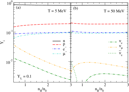
Figure 1: Particle fractions in neutron-star-merger matter, (lepton fraction $Y_{L}=0.1$). We plot $Y_{i}=n_{i}/n_{B}$ as functions of the baryon density $n_{B}$ for temperatures (a) $T=5$ MeV, and (b) $T=50$ MeV. At high temperature [panel (b)] the net electron neutrino density becomes negative at sufficiently low baryon density: the corresponding dotted line shows the net antineutrino fraction.

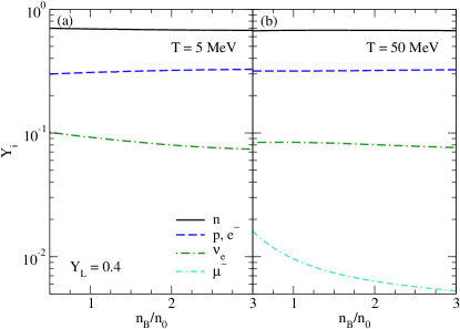
Figure 2: Particle fractions in supernova matter, (lepton fraction is $Y_{L}=0.4$ for electrons, and is zero for muons). We plot $Y_{i}=n_{i}/n_{B}$ as functions of the baryon density $n_{B}$ for temperatures (a) $T=5$ MeV, and (b) $T=50$ MeV. The particle fractions show little dependence on temperature.

Before presenting our results on the bulk viscosity in Sec. IV.2 we first discuss the thermodynamics of the underlying relativistic density functional model of nuclear matter, which will be used as the background equilibrium for our subsequent perturbation analysis. We will employ the DD-ME2 parametrization of the density functional given in Ref. Lalazissis2005 .

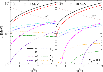
Figure 3: Chemical potentials in the neutron-star-merger matter, (lepton fraction $Y_{L}=0.1$). We plot $\mu_{i}$ as functions of the baryon density $n_{B}/n_{0}$ for temperatures (a) $T=5$ MeV, and (b) $T=50$ MeV. The labels $n^{*}$ and $p^{*}$ correspond to the effective chemical potentials of the neutron and proton, respectively, defined after Eq. (57). The effective baryon mass $m^{*}\equiv m_{B}^{*}$ is shown by the dotted lines.

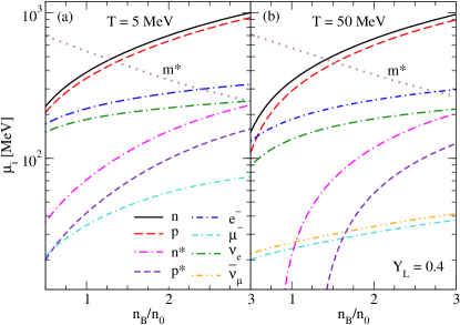
Figure 4: Chemical potentials in supernova matter, ($Y_{L}=0.4$ for electrons). We plot $\mu_{i}$ as functions of the baryon density $n_{B}/n_{0}$ for temperatures (a) $T=5$ MeV, and (b) $T=50$ MeV.

Figures 1 and 2 show the particle fractions $Y_{j}=n_{j}/n_{B}$ as functions of the baryon density normalized to the nuclear saturation density, which is $n_{0}=0.152$ fm^-3 in the DD-ME2 model. Figures 1 and 2 refer to the cases of neutron star mergers and supernovae, respectively. The results are shown for two temperatures $T=5$ MeV (which is of the order of $T_{\rm tr}$) [panels (a)] and $T=50$ MeV [panels (b)], which is close to the upper limit of the temperature range achieved in these events. Comparing the panels (a) and (b) in Figs. 1 and 2 we see that the particle fractions are generally not sensitive to the temperature for the given value of $Y_{L}$. The only exception is for low lepton-fraction matter, where at low density and high temperature (Fig. 1(b)), the net electron neutrino density becomes negative, indicating that there are more (electron) antineutrinos than neutrinos. As one would expect, merger (low lepton fraction) matter has much smaller electron neutrino fraction; the electron and muon fractions are $\sim 10\%$, so by charge neutrality $Y_{p}=Y_{e}+Y_{\mu}$ the proton fraction is $\sim 20\%$.

Since the bulk viscosity is related to departure from beta equilibrium, it is instructive to examine the chemical potentials of particles as functions of density and temperature. These are shown as functions of the baryon density in Figs. 3 and 4.

There are two different chemical potentials for baryons: the thermodynamic chemical potentials $\mu_{n}$ and $\mu_{p}$, which enter into the thermodynamic relations and the $\beta$-equilibrium condition (3), and the effective chemical potentials $\mu_{n}^{*}$ and $\mu_{p}^{*}$, which enter into the baryon distribution functions and are defined after Eq. (57). We show also the effective nucleon mass $m^{*}$ with dotted lines.

In low lepton-fraction matter at low density and high temperature (Fig. 3(b)), we see that the neutrino chemical potentials become negative, as expected from the particle fraction results (Fig. 1(b)) which showed that there are more antineutrinos than neutrinos in this regime.

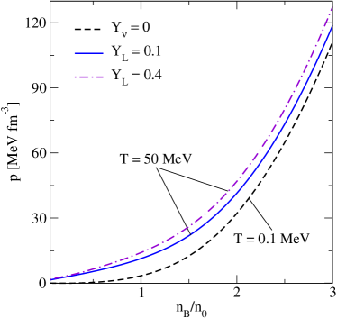
Figure 5: Equation of state of nuclear matter for several values of the lepton fraction and the temperature.

For completeness and reference, we show the equation of state (EoS) of the DD-ME2 model at two temperatures in Fig. 5. For $T=50$ MeV the EoS is shown for two values of lepton fractions corresponding to a supernova and binary-neutron-star merger settings. The increase in the pressure at larger temperatures is due to the additional thermal contribution from baryons and the contribution from trapped neutrinos which is absent in the case when $T=0.1$ MeV.

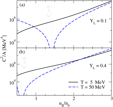
Figure 6: The ratio of beta-disequilibrium–baryon-density susceptibility (47) squared $C^{2}$ over $A$ as a function of the baryon density for two values of the temperature for (a) $Y_{L}=0.1$ and (b) $Y_{L}=0.4$.

IV.2 Perturbations and bulk viscosity

Now we turn to the discussion of perturbations on the background equilibrium of matter presented above and concentrate on the $\beta$-relaxation rates and the bulk viscosity.

Our numerical calculations show that the main contribution to the beta-disequilibrium–proton-fraction susceptibility $A$ (40) comes from neutrinos whereas electron contribution is minor. The baryon contributions are much smaller than those of leptons because of their finite mass, see Eq. (133). The contribution from $\rho$ meson is negligible in the whole regime of interest. The susceptibility $A$ does not depend strongly on the density and the temperature and has roughly the same order of magnitude $A\sim 10^{-3}$ MeV^-2 in the relevant portion of the phase diagram.

The beta-disequilibrium–proton-fraction susceptibility $C$ is an increasing function of density and has the same order of magnitude in the cases of neutron star mergers and supernovas. At sufficiently high temperatures $T\gtrsim 30$ MeV $C$ crosses zero at a temperature-dependent critical value of the density, close to saturation density. The vanishing of $C$ arises when the proton fraction in beta-equilibrated matter is independent of the density (passing through a minimum in this case). At the critical density the system is scale-invariant: it can be compressed and remain in beta equilibrium. Thus the bulk viscosity vanishes at the critical density.

Figure 6 shows the ratio $C^{2}/A$ as a function of density. As seen from the figure, this ratio is temperature-sensitive only close to the point were $C$ crosses zero.

In Appendix C we discuss the rates of neutron decay and electron capture that combine to establish beta equilibrium. Electron capture dominates because the neutron decay process involves antineutrinos the population of which is damped by a factor of $\exp(-\mu{{}_{\nu}}/T)$.

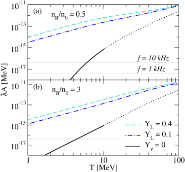
Figure 7: The beta-equilibration relaxation rate $\lambda A$ as a function of the temperature for fixed values of the lepton fraction for (a) $n_{B}/n_{0}=0.5$; (b) $n_{B}/n_{0}=3$. The horizontal lines correspond to fixed values of $\lambda A=\omega=2\pi f$ for the frequencies $f=1$ kHz (dashed line) and $f=10$ kHz (solid line). The black dotted lines show the extrapolation of our results for $Y_{\nu}=0$ case to the high-temperature regime $T\geq 10$ MeV where these are inapplicable.

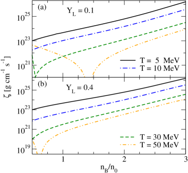
Figure 8: The density dependence of the bulk viscosity for various values of the temperature. The lepton fraction is $Y_{L}=0.1$ for panel (a) and $Y_{L}=0.4$ for panel (b).

In Fig. 7 we show the beta equilibrium relaxation rate $\lambda A$, which determines where the bulk viscosity reaches its resonant maximum [Eq. (53)]. For comparison here we show also the case of neutrino-transparent matter (solid line). The relaxation rate is slowest in the neutrino-transparent case and increases with the lepton fraction in the neutrino-trapped case.

The relaxation rate $\lambda A$ of the neutrino-trapped matter is several orders of magnitude larger than the oscillation frequencies $f=\omega/2\pi\lesssim 10$ kHz typical to neutron star mergers and supernovas. In Fig. 7 the horizontal lines for different oscillations frequencies intersect the $\lambda A$ curves at low temperatures $T\lesssim 0.1$ MeV, indicating that the resonant maximum occurs at low temperatures where the assumption of neutrino trapping is no longer valid. The neutrino-trapped regime lies at higher temperatures, where the bulk viscosity is independent of the oscillation frequency and takes the form $\zeta\approx C^{2}/(\lambda A^{2})$.

In contrast, the neutrino-transparent matter features bulk viscosity which strongly depends on the oscillation frequency, see Ref. Alford:2019zzz and Appendix D for details.

We also see from Fig. 7, that $\lambda A$ is almost independent of the baryon density in the range $0.5\leq n_{B}/n_{0}\leq 3$ for neutrino-trapped matter. At moderately temperatures $\lambda$ scales as $\lambda\propto T^{2}$ for temperatures $T\leq 10$ MeV: this scaling is clearly seen from Eqs. (22) and (24), which are applicable as long as the fermions are semidegenerate, i.e., $T\leq 10$ MeV in the relevant density range.

Figure 8 shows the density dependence of the bulk viscosity for various values of the temperature. Because the beta relaxation rate $\lambda A$ is almost independent of the baryon density, the density dependence of the bulk viscosity follows that of the susceptibility prefactor $C^{2}/A$, and, therefore, as noted above, may drop to zero at a critical density where the system becomes scale-invariant. The critical density is present only at sufficiently high temperatures $T\geq 30$ MeV.

The temperature dependence of the bulk viscosity is shown in Fig. 9. The temperature dependence of $\zeta$ arises mainly from the temperature dependence of the beta relaxation rate $\lambda A\propto T^{2}$ (see Eqs. (22) and (24)), so the bulk viscosity decreases as $\zeta\propto T^{-2}$ in the neutrino-trapped regime, as can be seen also from Fig. 9. This scaling breaks down at special temperatures where the bulk viscosity has zeros when the matter becomes scale-invariant (see our discussion of Fig. 6).

In order to check whether the high-temperature behavior found in Fig. 9 is a universal behavior or is specific to the EoS we used, we compared our results with those obtained in the framework of NL3 model, see Fig. 10. The figure shows that the minimums arise independently of the equation of state, and, therefore, are typical to the high-temperature regime of dense nuclear matter.

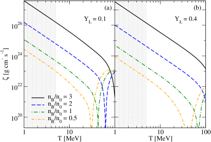
Figure 9: The temperature dependence of the bulk viscosity for DD-ME2 model or several values of the baryon density. The lepton fraction is fixed at $Y_{L}=0.1$ for panel (a) and at $Y_{L}=0.4$ for panel (b). The shaded region shows the extrapolation of our results to the neutrinoless regime $T\leq 5$ MeV where these are supposed to be inapplicable.

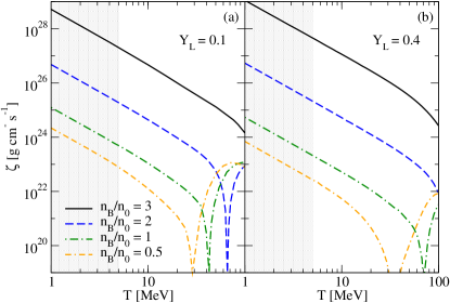
Figure 10: Same as Fig. 9 for model NL3.

Comparing the results shown in panels (a) and (b) of Figs. 8 and 9 we see that the bulk viscosity is generally by a factor of few smaller for larger lepton fractions, which is a consequence of larger values of $\lambda A$ for higher $Y_{L}$, as was seen from Fig. 7. However, the order of magnitude of the bulk viscosity is the same in both cases.

In Figs. 11 and 12 we combine and compare our results for the neutrino-trapped matter with the results for neutrino-transparent matter (see also Alford:2019zzz ). In the interval $5\leqslant T\leqslant 10$ MeV we interpolate the numerical results for the bulk viscosity between the two regimes. We see that the bulk viscosity in the neutrino transparent regime is larger, for two reasons. First, the beta relaxation rate is slower, so the resonant peak of the bulk viscosity occurs within its regime of validity, whereas for neutrino trapped matter the regime of validity starts at temperatures well above the resonant maximum. Second, the prefactor $C^{2}/A$ is larger in the neutrino-transparent matter, so the bulk viscosity reaches a higher value at its resonant maximum.

It, therefore, seems likely that bulk viscosity will have its greatest impact on neutron star mergers in regions of the merger that are neutrino transparent rather than neutrino trapped Alford:2019zzz .

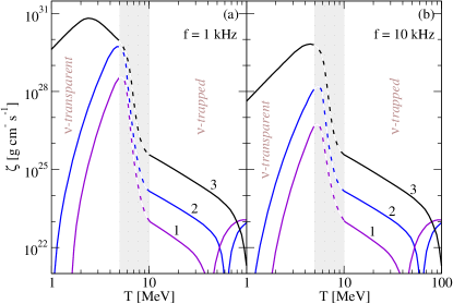
Figure 11: The bulk viscosity for DD-ME2 model for three values of the baryon density $n_{B}/n_{0}=1,2,3$ and for the lepton fraction $Y_{L}=0.1$. In the temperature range $5\leq T\leq 10$ MeV the bulk viscosity was interpolated between the results of $\nu$-transparent ($T\leq 5$ MeV) and $\nu$-trapped ($T\geq 10$ MeV) regimes. The oscillation frequency is fixed at (a) $f=1$ kHz and (b) $f=10$ kHz.

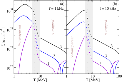
Figure 12: Same as Fig. 11 but for model NL3.

V Conclusions

In this work, we have studied the bulk viscosity of hadronic component of neutron stars composed of neutrons, protons, electrons, muons, and neutrinos. The main new ingredient of our study is the trapped neutrinos, which modify significantly the composition of the background equilibrium matter. We have derived semianalytical expressions for the weak interaction rates in the case of trapped neutrinos and corresponding expressions for the bulk viscosity. Our numerical study of the relevant quantities displays the following features:

(a) Electron capture dominates. In neutrino-trapped matter, beta equilibration, and hence bulk viscosity, is dominated by the electron capture process and its inverse (2). Neutron decay and its inverse (1) involve antineutrinos and are therefore suppressed by factors of $\exp(-\mu_{\nu}/T)$.

(b) Role of susceptibilities. The beta-disequilibrium–baryon-density susceptibility $C$ (47) plays an essential role in the bulk viscosity since it measures the degree to which matter is driven out of beta equilibrium when compressed at constant proton fraction (i.e., without any weak interactions). We find that $C$ vanishes, i.e., the proton fraction becomes independent of density, at a critical density that is in the vicinity of saturation density at high temperatures $T\gtrsim 30$ MeV. The subthermal bulk viscosity vanishes at this critical density because the equilibrium value of the proton fraction is density-independent, so compression does not drive the system out of beta equilibrium.

(c) Temperature dependence. The bulk viscosity as a function of temperature at fixed oscillation frequency $\omega$ shows the standard resonant form (53), with a maximum when the beta relaxation rate $\lambda A$ matches $\omega$. At the temperatures where our assumption of neutrino trapping is valid ($T\gtrsim 5\,{\rm MeV}$), we are always in the regime where beta relaxation is fast ($\lambda A$ is greater than typical frequencies for neutron star density oscillations, which are in the kHz range) so $\zeta\approx C^{2}/(\lambda A^{2})$. Since the relaxation rate rises with temperature (due to increasing phase space), the bulk viscosity drops with increasing temperature as $\zeta\propto T^{-2}$. This scaling can be understood, by noting that the factor $\lambda A$ scales approximately as $T^{-2}$. Given that the remaining factor $C^{2}/A$ mildly depends on the temperature (except the points where it goes to zero, see Fig. 6), we recover the $\zeta\propto T^{-2}$ scaling. At some temperatures and densities the material becomes scale-invariant, so $C$ goes through zero, driving the bulk viscosity to zero at those points.

(d) Dependence on lepton fraction. The dependence of the bulk viscosity on lepton fraction can be inferred from Figs. 8, 9, and 10. It is seen that the bulk viscosity is smaller for larger lepton fraction, specifically comparing the cases of supernova matter with $Y_{L}=0.4$ and neutron-star/binary-merger matter with $Y_{L}=0.1$ one finds that the bulk viscosity of supernova matter is a few times smaller compared to that of neutron-star/binary-merger matter.

(e) Effect of neutrino trapping. In astrophysical scenarios of supernova and binary-mergers, the object formed in the aftermath of these events will cool eventually below the neutrino trapping temperature $T_{\rm tr}$. Therefore, one may ask how the bulk viscosity of matter changes as it passes through $T_{\rm tr}$. Figure 11 shows the temperature dependence of the bulk viscosity, where we combine the results obtained in the neutrino-trapped ($T>T_{\rm tr}$) and neutrino-transparent matter ($T<T_{\rm tr}$). It is seen that the bulk viscosity of matter with neutrinos is several orders of magnitude smaller than that for the matter which is transparent to neutrinos.

(f) Dependence on the density-functional model. All computations have been carried out for two alternative relativistic density functional models one being the density-dependent DD-ME2 parametrization the other being the NL3 nonlinear parametrization. The key results show insignificant dependence on the chosen model, therefore we conclude that our results are largely independent of this input (see also Ref Yakovlev2018 ).

(g) Relevance for mergers. It seems likely that the presence of neutrino-trapped matter will not be an important source of bulk viscosity in mergers. Ref. Alford:2019zzz found that the bulk viscosity in neutrino transparent matter was just enough to yield dissipation times in the 20 ms range. We find that bulk viscosity in neutrino-trapped matter is thousands of times smaller, so the corresponding dissipation times are likely to be too long to affect a merger, provided other input in the analysis of Ref. Alford:2019zzz does not change by orders of magnitude.

In the future it would be interesting to extend our discussion to more complicated compositions of dense matter which would include heavy baryons such as hyperons and delta-isobars Li2018_PLB ; Li2019ApJ . We also hope that this work will help to clarify which dissipative processes are important enough to be worth including in hydrodynamic simulations of neutron star mergers.

Appendix A Phase space integrals

For further computations it is convenient to write the energy conservation in the form $\delta(p_{0}\pm k_{0}+k^{\prime}_{0}-p^{\prime}_{0})=\delta(\epsilon_{p}\pm\epsilon_{\bar{\nu}/\nu}+\epsilon_{e}-\epsilon_{n}-\mu_{\Delta})$, where we added and subtracted $\mu_{\Delta}$ in the argument of the $\delta$-function, and denoted by $\epsilon_{i}$ the energies of the particles computed from their chemical potentials, e.g., $\epsilon_{p}=p_{0}-\mu_{p}$. To simplify the calculation of the $\beta$-equilibration rates it is useful to introduce a so-called “dummy” integration, so that, by substituting Eq. (7) into the rates (8) and (18) we obtain

$$\Gamma_{1p}(\mu_{\Delta}) = 2\tilde{G}^{2}\int d^{4}qI_{1}(q)\,I_{2}(q),$$ (61)

$$\Gamma_{2p}(\mu_{\Delta}) = 2\tilde{G}^{2}\int d^{4}qI_{1}(q)\,I_{3}(q),$$ (62)

where

$$I_{1}(q) = \int\!\!\frac{d^{3}p^{\prime}}{(2\pi)^{3}}\int\!\!\frac{d^{3}p}{(2\pi)^{3}}[1-f(p)]f(p^{\prime})(2\pi)^{4}\delta^{(4)}(p-p^{\prime}+q),$$ (63)

$$I_{2}(q) = \int\!\!\frac{d^{3}k^{\prime}}{(2\pi)^{3}}\int\!\!\frac{d^{3}k}{(2\pi)^{3}}[1-f(k^{\prime})][1-f(k)]\delta^{(4)}(k+k^{\prime}-q),$$ (64)

$$I_{3}(q) = \int\!\!\frac{d^{3}k^{\prime}}{(2\pi)^{3}}\int\!\!\frac{d^{3}k}{(2\pi)^{3}}f(k)[1-f(k^{\prime})]\delta^{(4)}(k^{\prime}-k-q),$$ (65)

with $\delta^{(4)}(p-p^{\prime}+q)=\delta({\bm{p}}-{\bm{p}}^{\prime}+{\bm{q}})\delta(\epsilon_{p}-\epsilon_{p^{\prime}}+\omega-\mu_{\Delta})$, $\delta^{(4)}(k^{\prime}\pm k-q)=\delta({\bm{k}}^{\prime}\pm{\bm{k}}-{\bm{q}})\delta(\epsilon_{k^{\prime}}\pm\epsilon_{k}-\omega)$. The rates of the inverse processes (9) and (19) can be obtained from Eqs. (61) and (62) by replacing $f(p_{i})\to 1-f(p_{i})$ for all particles. Thus, the problem reduces to the computation of three $q$-dependent integrals $I_{1}(q)$, $I_{2}(q)$ and $I_{3}(q)$ in Eq. (63)-(65).

To compute the integral $I_{1}(q)$ we use the following identity between the Fermi $f(p)$ and Bose $g(p)$ functions

$$f(p^{\prime})[1-f(p)]=g(q)[f(p)-f(p^{\prime})].$$ (66)

Then, integrating over neutron momentum and separating the angular part of the remaining integral we obtain ($\tilde{\omega}=\omega-\mu_{\Delta}$)

$$I_{1}(q)=(2\pi)^{-1}g(q)\int_{0}^{\infty}\!dp\,p^{2}[f(\epsilon_{p})-f(\epsilon_{p}+\tilde{\omega})]\int_{-1}^{1}dx\,\delta(\tilde{\omega}+\epsilon_{p}-\epsilon_{p+q}),$$ (67)

where $x$ is the cosine of the angle between $\bm{p}$ and $\bm{q}$. Using the nonrelativistic spectrum for the nucleons $\epsilon_{i}=p^{2}/2m^{*}-\mu_{i}^{*}$, $i=\{p,n\}$, we obtain for $I_{1}(q)$

$$I_{1}(q)=(2\pi)^{-1}g(q)\int_{0}^{\infty}\!dp\,p^{2}[f(\epsilon_{p})-f(\epsilon_{p}+\tilde{\omega})]\frac{m^{*}}{pq}\theta(1-|x_{0}|),$$ (68)

where $x_{0}$ is the zero of the argument of the $\delta$-function, i.e.,

$$x_{0}=\frac{m^{*}}{pq}\left(\mu_{n}^{*}-\mu_{p}^{*}+\tilde{\omega}-\frac{q^{2}}{2m^{*}}\right).$$ (69)

The step-function sets the following limit on the momentum of a particle

$$p\geq p_{\rm min}=\frac{m^{*}}{q}\left|\mu_{n}^{*}-\mu_{p}^{*}+\tilde{\omega}-\frac{q^{2}}{2m^{*}}\right|.$$ (70)

Taking now the momentum integral we finally obtain (note that $g(q)$ depends only on $\omega$)

$$I_{1}(q)=g(\tilde{\omega})\frac{m^{*2}}{2\pi q}\int_{\epsilon_{\rm min}}^{\infty}d\epsilon_{p}\left[f(\epsilon_{p})-f(\epsilon_{p}+\tilde{\omega})\right]=g(\omega-\mu_{\Delta})\frac{m^{*2}T}{2\pi q}\ln\Bigg{|}\frac{1+\exp\left(-\frac{\epsilon_{\rm min}}{T}\right)}{1+\exp\left(-\frac{\epsilon_{\rm min}+\omega-\mu_{\Delta}}{T}\right)}\Bigg{|},$$ (71)

where the lower limit $\epsilon_{\rm min}$ follows from $p_{\rm min}$, i.e.,

$$\epsilon_{\rm min}=\frac{p_{\rm min}^{2}}{2m^{*}}-\mu_{p}^{*}=\frac{m^{*}}{2q^{2}}\bigg{(}\mu_{n}^{*}-\mu_{p}^{*}+\omega-\mu_{\Delta}-\frac{q^{2}}{2m^{*}}\bigg{)}^{2}-\mu_{p}^{*}.$$ (72)

We now transform the second integral (64)

$$I_{2}(q) = \int\!\!\frac{d^{3}k^{\prime}}{(2\pi)^{3}}\int\!\!\frac{d^{3}k}{(2\pi)^{3}}[1-f(k^{\prime})][1-f(k)]\delta(\epsilon_{k^{\prime}}+\epsilon_{k}-\omega)\delta({\bm{k}}+{\bm{k}}^{\prime}-{\bm{q}})$$ (73)

$$= \int\!\!\frac{k^{2}dk}{(2\pi)^{5}}[1-f(\omega-\epsilon_{k})][1-f(\epsilon_{k})]\int_{-1}^{1}dy\,\delta\left(k+\sqrt{k^{2}+q^{2}-2kqy}-\omega^{\prime}\right),$$

where we neglected the electron mass and introduced the short-hand notation $\omega^{\prime}=\omega+\mu_{e}-\mu_{\nu}$. The argument of the $\delta$-function is zero at

$$y_{0}=\frac{q^{2}-\omega^{\prime 2}+2\omega^{\prime}k}{2kq},$$ (74)

therefore for the $\delta$-function, we obtain (note that the $\delta$-function also implies $\omega^{\prime}-k\geq 0$)

$$\delta\left(k+\sqrt{k^{2}+q^{2}-2kqy}-\omega^{\prime}\right)=\frac{\omega^{\prime}-k}{kq}\theta(\omega^{\prime}-k)\delta(y-y_{0}),$$ (75)

and

$$\int_{-1}^{1}dy\delta\left(k+\sqrt{k^{2}+q^{2}-2kqy}-\omega^{\prime}\right)=\frac{\omega^{\prime}-k}{kq}\theta(\omega^{\prime}-k)\theta(1-|y_{0}|).$$ (76)

The condition $|y_{0}|\leq 1$ sets the following limits on the momentum $k$

$$-2kq\leq q^{2}-\omega^{\prime 2}+2\omega^{\prime}k\leq 2kq,$$ (77)

therefore the following two inequalities must be satisfied simultaneously

$$(\omega^{\prime}+q)(q-\omega^{\prime}+2k)\geq 0,\qquad(\omega^{\prime}-q)(q+\omega^{\prime}-2k)\geq 0.$$ (78)

Note that because of the condition $\omega^{\prime}\geq k\geq 0$ we have $\omega^{\prime}+q\geq 0$. Then the first condition in Eq. (78) gives $k\geq(\omega^{\prime}-q)/2$. Next, if $\omega^{\prime}\geq q$, the second condition implies $k\leq(\omega^{\prime}+q)/2\leq\omega^{\prime}$. If $\omega^{\prime}\leq q$ instead, then the first condition is satisfied automatically, and the second one gives $k\geq(\omega^{\prime}+q)/2\geq\omega^{\prime}$, which is not allowed. Substituting these results into Eq. (73) we obtain

$$I_{2}(q)=\theta(\omega^{\prime}-q)\frac{1}{q(2\pi)^{5}}\int_{(\omega^{\prime}-q)/2}^{(\omega^{\prime}+q)/2}kdk\,(\omega^{\prime}-k)[1-f(\omega-\epsilon_{k})][1-f({\epsilon}_{k})].$$ (79)

The integral $I_{3}(q)$ given by Eq. (65) is transformed as follows

$$I_{3}(q) = \int\!\!\frac{d^{3}k^{\prime}}{(2\pi)^{3}}\int\!\!\frac{d^{3}k}{(2\pi)^{3}}f(k)[1-f(k^{\prime})]\delta(\epsilon_{k^{\prime}}-\epsilon_{k}-\omega)\delta({\bm{k}}^{\prime}-{\bm{k}}-{\bm{q}})$$ (80)

$$= \int\!\!\frac{k^{2}dk}{(2\pi)^{5}}f(\epsilon_{k})[1-f(\epsilon_{k}+\omega)]\int_{-1}^{1}dy\,\delta\left(-k+\sqrt{k^{2}+q^{2}+2kqy}-\omega^{\prime}\right).$$

The argument of the $\delta$-function is zero at

$$y_{0}=-\frac{q^{2}-\omega^{\prime 2}-2\omega^{\prime}k}{2kq},$$ (81)

and for the $\delta$-function we obtain (note that the $\delta$-function also implies $\omega^{\prime}+k\geq 0$)

$$\delta\left(-k+\sqrt{k^{2}+q^{2}+2kqy}-\omega^{\prime}\right)=\frac{\omega^{\prime}+k}{kq}\theta(\omega^{\prime}+k)\delta(y-y_{0}),$$ (82)

therefore

$$\int_{-1}^{1}dy\delta\left(-k+\sqrt{k^{2}+q^{2}+2kqy}-\omega^{\prime}\right)=\frac{\omega^{\prime}+k}{kq}\theta(\omega^{\prime}+k)\theta(1-|y_{0}|).$$ (83)

The condition $|y_{0}|\leq 1$ sets the following limits on the momentum $k$

$$-2kq\leq q^{2}-\omega^{\prime 2}-2\omega^{\prime}k\leq 2kq,$$ (84)

therefore the following two inequalities must be satisfied simultaneously

$$(\omega^{\prime}+q)(q-\omega^{\prime}-2k)\leq 0,\qquad(\omega^{\prime}-q)(q+\omega^{\prime}+2k)\leq 0.$$ (85)

Because of the condition $\omega^{\prime}+k\geq 0$ we have $\omega^{\prime}+q+2k\geq 0$. Then the second condition in Eq. (85) gives $q\geq\omega^{\prime}$. Next, if $\omega^{\prime}\geq-q$, the first condition implies $k\geq(q-\omega^{\prime})/2\geq-\omega^{\prime}$. If $\omega^{\prime}\leq-q$ instead, then the first condition implies $k\leq(q-\omega^{\prime})/2\leq-\omega^{\prime}$, which is not allowed. Substituting these results into Eq. (80) we obtain

$$I_{3}(q)=\theta(q-|\omega^{\prime}|)\frac{1}{q(2\pi)^{5}}\int_{(q-\omega^{\prime})/2}^{\infty}kdk\,(\omega^{\prime}+k)f(\epsilon_{k})[1-f(\epsilon_{k}+\omega)].$$ (86)

Combining now Eqs. (61), (62), (71), (79) and (86) we obtain the final formulas for $\Gamma_{1p}$ and $\Gamma_{2p}$ given in the main text by Eqs. (10) and (20). The rates of the inverse processes $\Gamma_{1n}$ and $\Gamma_{2n}$ given by Eqs. (11) and (21) can be obtained in an analogous manner.

For the derivatives of the rates $\Gamma_{1p}$ and $\Gamma_{1n}$ we obtain

$$\frac{\partial\Gamma_{1p}(\mu_{\Delta})}{\partial\mu_{\Delta}}\bigg{|}_{\mu_{\Delta}=0} = \frac{m^{*2}\tilde{G}^{2}}{8\pi^{5}}T^{5}\int_{-\alpha_{e}+\alpha_{\nu}}^{\infty}dy\,g(y)\int_{0}^{y+\alpha_{e}-\alpha_{\nu}}dz\,\bigg{\{}[1+g(y)]\ln\Bigg{|}\frac{1+\exp\left(-y_{0}\right)}{1+\exp\left(-y_{0}-y\right)}\Bigg{|}$$ (87)

$$-f(y_{0}+y)-\left[f(y_{0}+y)-f(y_{0})\right]\frac{m^{*}}{z^{2}T}\bigg{(}\alpha_{n}-\alpha_{p}+y-z^{2}\frac{T}{2m^{*}}\bigg{)}\bigg{\}}$$

$$\times\int_{x_{\rm min}}^{x_{\rm max}}dx\,(x-\alpha_{\nu})(y+\alpha_{e}-x)[1-f(x)]f(x-y),$$

$$\frac{\partial\Gamma_{1n}(\mu_{\Delta})}{\partial\mu_{\Delta}}\bigg{|}_{\mu_{\Delta}=0} = \frac{m^{*2}\tilde{G}^{2}}{8\pi^{5}}T^{5}\int_{-\alpha_{e}+\alpha_{\nu}}^{\infty}dy\,[1+g(y)]\int_{0}^{y+\alpha_{e}-\alpha_{\nu}}dz\,\bigg{\{}g(y)\ln\Bigg{|}\frac{1+\exp\left(-y_{0}\right)}{1+\exp\left(-y_{0}-y\right)}\Bigg{|}$$ (88)

$$-f(y_{0}+y)-\left[f(y_{0}+y)-f(y_{0})\right]\frac{m^{*}}{z^{2}T}\bigg{(}\alpha_{n}-\alpha_{p}+y-z^{2}\frac{T}{2m^{*}}\bigg{)}\bigg{\}}$$

$$\int_{x_{\rm min}}^{x_{\rm max}}dx\,(x-\alpha_{\nu})(y+\alpha_{e}-x)f(x)[1-f(x-y)].$$

In the same way we obtain for $\Gamma_{2p}$ and $\Gamma_{2n}$

$$\frac{\partial\Gamma_{2p}(\mu_{\Delta})}{\partial\mu_{\Delta}}\bigg{|}_{\mu_{\Delta}=0} = \frac{m^{*2}\tilde{G}^{2}}{8\pi^{5}}T^{5}\int_{-\infty}^{\infty}dy\,g(y)\int_{|y+\alpha_{e}-\alpha_{\nu}|}^{\infty}dz\,\Bigg{\{}[1+g(y)]\ln\bigg{|}\frac{1+\exp\left(-y_{0}\right)}{1+\exp\left(-y_{0}-y)\right)}\bigg{|}$$ (89)

$$-f(y_{0}+y)-[f(y_{0}+y)-f(y_{0})]\frac{m^{*}}{z^{2}T}\bigg{(}\alpha_{n}-\alpha_{p}+y-z^{2}\frac{T}{2m^{*}}\bigg{)}\Bigg{\}}$$

$$\times\int_{\bar{x}_{\rm min}}^{\infty}dx\,(x+\alpha_{\nu})(y+\alpha_{e}+x)f(x)[1-f(x+y)],$$

$$\frac{\partial\Gamma_{2n}(\mu_{\Delta})}{\partial\mu_{\Delta}}\bigg{|}_{\mu_{\Delta}=0} = \frac{m^{*2}\tilde{G}^{2}}{8\pi^{5}}T^{5}\int_{-\infty}^{\infty}dy\,[1+g(y)]\int_{|y+\alpha_{e}-\alpha_{\nu}|}^{\infty}dz\,\Bigg{\{}g(y)\ln\bigg{|}\frac{1+\exp\left(-y_{0}\right)}{1+\exp\left(-y_{0}-y)\right)}\bigg{|}$$ (90)

$$-f(y_{0}+y)-[f(y_{0}+y)-f(y_{0})]\frac{m^{*}}{z^{2}T}\bigg{(}\alpha_{n}-\alpha_{p}+y-z^{2}\frac{T}{2m^{*}}\bigg{)}\Bigg{\}}$$

$$\times\int_{\bar{x}_{\rm min}}^{\infty}dx\,(x+\alpha_{\nu})(y+\alpha_{e}+x)f(x+y)[1-f(x)].$$

From these expressions, it is straightforward to obtain Eqs. (13), (15), (22) and (25) of the main text.

A.1 Low-temperature Urca rates

In the case of highly degenerate matter we have $\mu_{i}/T\to\infty$, therefore $\epsilon_{\rm min}/T\to\pm\infty$. Thus we find from Eq. (71) (for $\mu_{\Delta}=0$)

$$I_{1}(q)=\frac{m^{*2}\omega}{2\pi q}g(\omega)\theta(-\epsilon_{\rm min}).$$ (91)

In terms of momenta the condition $\epsilon_{\rm min}\leq 0$ can be written as $|p_{Fn}^{2}-p_{Fp}^{2}-q^{2}|\leq 2qp_{Fp}$, where we neglected $\omega\sim T$ terms, therefore

$$\theta(-\epsilon_{\rm min})=\theta(p_{Fn}+p_{Fp}-q)\theta(q-|p_{Fn}-p_{Fp}|).$$ (92)

In the case of neutrino-transparent matter, we can also set $q=p_{Fe}$, therefore for Eq. (91) we obtain

$$I_{1}(q)=\frac{m^{*2}\omega}{2\pi q}g(\omega)\theta(p_{Fp}+p_{Fe}-p_{Fn}).$$ (93)

To obtain the low-temperature limit of integral $I_{2}$ in the case of neutrino-transparent matter we drop the neutrino momentum and neutrino distribution and approximate $|\bm{k}^{\prime}|=p_{Fe}$ in the first equation of (73), which gives

$$I_{2}(q)=\int\!\!\frac{k^{2}dk}{(2\pi)^{3}}\int\!\!\frac{dk^{\prime}}{(2\pi)^{3}}[1-f(k^{\prime})]\int d\Omega_{k}\,\delta(\epsilon_{k^{\prime}}+\epsilon_{k}-\omega)\delta(p_{Fe}-|{\bm{q}}|).$$ (94)

Performing the integrations over $k^{\prime}$ and $\Omega_{k}$ we obtain

$$I_{2}(q)=\frac{4\pi}{(2\pi)^{6}}\delta(p_{Fe}-|{\bm{q}}|)\int_{0}^{\infty}\!\!dk\,k^{2}[1-f(\omega-\epsilon_{k})].$$ (95)

Substituting Eqs. (93) and (95) into the neutron decay rate (61) we find

$$\Gamma_{1p}=\frac{m^{*2}\tilde{G}^{2}}{4\pi^{5}}T^{5}p_{Fe}\theta(p_{Fp}+p_{Fe}-p_{Fn})\int_{0}^{\infty}\!\!dx\,x^{2}\int_{-\infty}^{\infty}dy\,yg(y)f(x-y).$$ (96)

In the same manner we can obtain the low-$T$ result for $\Gamma_{2n}$ in the neutrino-transparent matter

$$\Gamma_{2n}=\frac{m^{*2}\tilde{G}^{2}}{4\pi^{5}}T^{5}p_{Fe}\theta(p_{Fp}+p_{Fe}-p_{Fn})\int_{0}^{\infty}\!\!dx\,x^{2}\int_{-\infty}^{\infty}dy\,y[1+g(y)]f(x+y).$$ (97)

The integrals appearing in Eqs. (96) and (97) can be computed successively

$$\int\limits_{-\infty}^{\infty}dy\ yg(y)f(x-y)=\int_{-\infty}^{\infty}dy\,y[1+g(y)]f(x+y)=\frac{1}{2}\frac{x^{2}+\pi^{2}}{1+e^{x}},$$ (98)

and

$$\frac{1}{2}\int_{0}^{\infty}dx\ x^{2}\frac{x^{2}+\pi^{2}}{1+e^{x}}=\frac{3}{4}\left[\pi^{2}\zeta(3)+15\zeta(5)\right]=20.5633,$$ (99)

from which we obtain the low-$T$ results (16) and (26) of the main text.

Next, we find the low-temperature limit of Eqs. (15) and (25). By replacing $\omega\to\omega-\mu_{\Delta}$ in Eq. (93) we find

$$\frac{\partial I_{1}}{\partial\mu_{\Delta}}\bigg{|}_{\mu_{\Delta}=0}=\Big{(}\frac{\omega}{T}[1+g(\omega)]-1\Big{)}\frac{m^{*2}}{2\pi q}g(\omega)\theta(p_{Fp}+p_{Fe}-p_{Fn}).$$ (100)

Therefore, the low-temperature limit for $\lambda_{1}$ can be found by replacing $y\to\{y[1+g(y)]-1\}/T$ in Eq. (96). Thus

$$\lambda_{1}=\frac{m^{*2}\tilde{G}^{2}}{4\pi^{5}}T^{4}p_{Fe}\theta(p_{Fp}+p_{Fe}-p_{Fn})\int_{0}^{\infty}dx\,x^{2}\int_{-\infty}^{\infty}dy\,g(y)\big{\{}y[1+g(y)]-1\big{\}}f(x-y).$$ (101)

Similarly, $\lambda_{2}$ can be obtained from Eq. (97) by replacing $y\to-[yg(y)-1]/T$

$$\lambda_{2}=\frac{m^{*2}\tilde{G}^{2}}{4\pi^{5}}T^{4}p_{Fe}\theta(p_{Fp}+p_{Fe}-p_{Fn})\int_{0}^{\infty}dx\,x^{2}\int_{-\infty}^{\infty}dy\,[1+g(y)][1-yg(y)]f(x+y).$$ (102)

The double integrals in Eqs. (101) and (102) are identical and are equal to $17\pi^{4}/120$. Substituting this value we obtain the final results given by Eqs. (17) and (27).

In the case where neutrinos remain trapped in the degenerate regime, one finds $I_{2}(q)=0$, because in this limit the distribution function of antineutrinos is exponentially suppressed. To obtain the low-temperature limit of $I_{3}(q)$ we substitute $k=p_{F\nu}$ and $\omega^{\prime}=\mu_{e}-\mu_{\nu}=p_{Fe}-p_{F\nu}$ in Eq. (86) ($\epsilon_{k}\equiv k-p_{F\nu}$) to find

$$I_{3}(q)=\frac{p_{Fe}p_{F\nu}}{q(2\pi)^{5}}\theta(1-|y_{0}|)\int_{-p_{F\nu}}^{\infty}d\epsilon_{k}\,f(\epsilon_{k})[1-f(\epsilon_{k}+\omega)].$$ (103)

The inequalities (85) in this approximation are independent of $\epsilon_{k}$ and imply

$$|p_{Fe}-p_{F\nu}|\leq q\leq p_{Fe}+p_{F\nu}.$$ (104)

Combining now Eqs. (62), (91) and (103) and approximating $p_{F\nu}/T\to\infty$ for $\Gamma_{2}$ we obtain

$$\Gamma_{2}=\frac{m^{*2}\tilde{G}^{2}}{8\pi^{5}}T^{3}p_{Fe}p_{F\nu}\int_{|p_{Fe}-p_{F\nu}|}^{p_{Fe}+p_{F\nu}}dq\,\theta(p_{Fn}+p_{Fp}-q)\theta(q-|p_{Fn}-p_{Fp}|)\int_{-\infty}^{\infty}dx\,f(x)\int_{-\infty}^{\infty}dy\,yg(y)f(-x-y).\quad$$ (105)

The last two integrals give $2\pi^{2}/3$, and for the $q$-integral we have

$$\int_{|p_{Fe}-p_{F\nu}|}^{p_{Fe}+p_{F\nu}}dq~{}\theta(p_{Fn}+p_{Fp}-q)\theta(q-|p_{Fn}-p_{Fp}|)$$

$$=(p_{Fe}+p_{F\nu}-|p_{Fn}-p_{Fp}|)\theta(p_{Fn}+p_{Fp}-p_{Fe}-p_{F\nu})\theta(p_{Fe}+p_{F\nu}-|p_{Fn}-p_{Fp}|)\theta(|p_{Fn}-p_{Fp}|-|p_{Fe}-p_{F\nu}|)$$

$$+(p_{Fn}+p_{Fp}-|p_{Fe}-p_{F\nu}|)\theta(p_{Fe}+p_{F\nu}-p_{Fn}-p_{Fp})\theta(p_{Fn}+p_{Fp}-|p_{Fe}-p_{F\nu}|)\theta(|p_{Fe}-p_{F\nu}|-|p_{Fn}-p_{Fp}|)$$

$$+(p_{Fe}+p_{F\nu}-|p_{Fe}-p_{F\nu}|)\theta(p_{Fn}+p_{Fp}-p_{Fe}-p_{F\nu})\theta(|p_{Fe}-p_{F\nu}|-|p_{Fn}-p_{Fp}|)$$

$$+(p_{Fn}+p_{Fp}-|p_{Fn}-p_{Fp}|)\theta(p_{Fe}+p_{F\nu}-p_{Fn}-p_{Fp})\theta(|p_{Fn}-p_{Fp}|-|p_{Fe}-p_{F\nu}|).$$ (106)

In neutron star matter we have typically $p_{Fn}+p_{Fp}\geq p_{Fe}+p_{F\nu}\geq|p_{Fn}-p_{Fp}|\geq|p_{Fe}-p_{F\nu}|$, and we obtain the final result given by Eq. (24).

Appendix B Computation of susceptibilities $A_{j}$

To compute the susceptibilities $A_{ij}$ given by Eq. (32) we use the following formula for the particle densities

$$n_{i}=\frac{g_{i}}{2\pi^{2}}\int_{0}^{\infty}p^{2}dp\,[f_{i}(p)-\bar{f}_{i}(p)],$$ (107)

where $g_{i}$ is the degeneracy factor, and $f(p)$ and $\bar{f}(p)$ are the distribution functions for particles and antiparticles, respectively. For neutrons, protons, and electrons we have $g_{i}=2$, and for neutrinos $g_{\nu}=1$.

Differentiating the left and right sides of Eq. (107) with respect to $n_{j}$ and exploiting the expressions

$$\frac{\partial f_{i}}{\partial n_{j}}=-f_{i}(1-f_{i})\frac{1}{T}\left(\frac{m^{*}}{\sqrt{m^{*2}+p^{2}}}\frac{\partial m^{*}}{\partial n_{j}}-\frac{\partial\mu^{*}_{i}}{\partial n_{j}}\right),\qquad\frac{\partial\bar{f}_{i}}{\partial n_{j}}=-\bar{f}_{i}(1-\bar{f}_{i})\frac{1}{T}\left(\frac{m^{*}}{\sqrt{m^{*2}+p^{2}}}\frac{\partial m^{*}}{\partial n_{j}}+\frac{\partial\mu^{*}_{i}}{\partial n_{j}}\right),$$ (108)

in the case of baryons we obtain

$$\delta_{ij}=-\left(\frac{\partial m^{*}}{\partial n_{j}}\right){I}_{1i}^{-}+\left(\frac{\partial\mu^{*}_{i}}{\partial n_{j}}\right){I}_{0i}^{+},$$ (109)

where

$${I}^{\pm}_{qi}=\frac{1}{\pi^{2}T}\int_{0}^{\infty}p^{2}dp\left(\frac{m^{*}}{\sqrt{m^{*2}+p^{2}}}\right)^{q}[f_{i}(1-f_{i})\pm\bar{f}_{i}(1-\bar{f}_{i})],\quad i=\{n,p\}.$$ (110)

The average values of the meson fields are given by Chatterjee2007

$$g_{\omega}\omega_{0}=\left(\frac{g_{\omega}}{m_{\omega}}\right)^{2}(n_{n}+n_{p}),\qquad g_{\rho}\rho_{03}=\frac{1}{2}\left(\frac{g_{\rho}}{m_{\rho}}\right)^{2}(n_{p}-n_{n}),$$ (111)

which gives (recall that $\mu^{*}_{i}=\mu_{i}-g_{\omega}\omega_{0}-g_{\rho}\rho_{03}I_{3i}$)

$$B_{ij}\equiv\frac{\partial\mu^{*}_{i}}{\partial n_{j}}=A_{ij}-\left(\frac{g_{\omega}}{m_{\omega}}\right)^{2}-I_{3i}I_{3j}\left(\frac{g_{\rho}}{m_{\rho}}\right)^{2}.$$ (112)

The scalar field is given by

$$g_{\sigma}\sigma=m-m^{*}=-\frac{g_{\sigma}}{m_{\sigma}^{2}}\frac{\partial U(\sigma)}{\partial\sigma}+\frac{1}{\pi^{2}}\left(\frac{g_{\sigma}}{m_{\sigma}}\right)^{2}\sum_{i=n,p}\int_{0}^{\infty}p^{2}dp\frac{m^{*}}{\sqrt{p^{2}+m^{*2}}}[f_{i}(p)+\bar{f}_{i}(p)],$$ (113)

with $U(\sigma)$ being the self-interaction potential of the scalar field, therefore

$$\frac{\partial m^{*}}{\partial n_{j}}=\frac{g_{\sigma}}{m_{\sigma}^{2}}\frac{\partial^{2}U(\sigma)}{\partial\sigma^{2}}\frac{\partial\sigma}{\partial n_{j}}+\left(\frac{g_{\sigma}}{m_{\sigma}}\right)^{2}\left(\frac{\partial m^{*}}{\partial n_{j}}\right)\left({I}_{2n}^{+}+{I}_{2p}^{+}\right)-\left(\frac{g_{\sigma}}{m_{\sigma}}\right)^{2}\left(B_{nj}{I}_{1n}^{-}+B_{pj}{I}_{1p}^{-}\right)$$

$$-\left(\frac{g_{\sigma}}{m_{\sigma}}\right)^{2}\left(\frac{\partial m^{*}}{\partial n_{j}}\right)\sum_{i=n,p}\frac{1}{\pi^{2}}\int_{0}^{\infty}p^{2}dp\frac{p^{2}}{(p^{2}+m^{*2})^{3/2}}[f_{i}(p)+\bar{f}_{i}(p)].$$ (114)

The last term is suppressed in the nonrelativistic limit and can be neglected, after which we obtain

$$\frac{\partial m^{*}}{\partial n_{j}}=-\frac{\left(\frac{g_{\sigma}}{m_{\sigma}}\right)^{2}\left(B_{nj}{I}_{1n}^{-}+B_{pj}{I}_{1p}^{-}\right)}{1-\left(\frac{g_{\sigma}}{m_{\sigma}}\right)^{2}\left({I}_{2n}^{+}+{I}_{2p}^{+}\right)+\frac{1}{m_{\sigma}^{2}}\frac{\partial^{2}U}{\partial\sigma^{2}}}.$$ (115)

Substituting this into Eq. (109) we obtain the following equations for coefficients $B_{ij}$

$$B_{ij}{I}_{0i}^{+}-\gamma\left(B_{nj}{I}_{1n}^{-}+B_{pj}{I}_{1p}^{-}\right){I}_{1i}^{-}=\delta_{ij},$$ (116)

where

$$\gamma=\frac{1}{{I}_{2n}^{+}+{I}_{2p}^{+}-\beta},\qquad\beta=\left(\frac{m_{\sigma}}{g_{\sigma}}\right)^{2}\left(1+\frac{1}{m_{\sigma}^{2}}\frac{\partial^{2}U}{\partial\sigma^{2}}\right).$$ (117)

In the case of $i\neq j$ we find from Eq. (116)

$$B_{np}=\gamma B_{pp}\frac{I_{1p}^{-}I_{1n}^{-}}{I_{0n}^{+}-\gamma I_{1n}^{-2}},\qquad B_{pn}=\gamma B_{nn}\frac{I_{1n}^{-}I_{1p}^{-}}{I_{0p}^{+}-\gamma I_{1p}^{-2}}.$$ (118)

Substituting these expressions into Eq. (116) for $i=j$ we obtain

$$B_{nn}=\frac{I_{0p}^{+}-\gamma I_{1p}^{-2}}{I_{0n}^{+}I_{0p}^{+}-\gamma I_{0p}^{+}I_{1n}^{-2}-\gamma I_{0n}^{+}I_{1p}^{-2}},\qquad B_{pp}=\frac{I_{0n}^{+}-\gamma I_{1n}^{-2}}{I_{0n}^{+}I_{0p}^{+}-\gamma I_{0p}^{+}I_{1n}^{-2}-\gamma I_{0n}^{+}I_{1p}^{-2}},$$ (119)

and

$$B_{np}=B_{pn}=\frac{\gamma I_{1p}^{-}I_{1n}^{-}}{I_{0n}^{+}I_{0p}^{+}-\gamma I_{0p}^{+}I_{1n}^{-2}-\gamma I_{0n}^{+}I_{1p}^{-2}}.$$ (120)

In the nonrelativistic limit we will use the expansion $m/\sqrt{m^{2}+p^{2}}\simeq 1-p^{2}/2m^{2}$ in the integrals (110). We will further drop the contribution of antiparticles because it is not important for the regime of interest. Then ${I}_{0i}^{+}={I}_{0i}^{-}\simeq\tilde{I}_{2i}$, ${I}_{1i}^{+}={I}_{1i}^{-}\simeq\tilde{I}_{2i}-\tilde{I}_{4i}/2m^{*2}$, and ${I}_{2i}^{+}={I}_{2i}^{-}\simeq\tilde{I}_{2i}-\tilde{I}_{4i}/m^{*2}$, where

$$\tilde{I}_{qi}=\frac{1}{\pi^{2}T}\int_{0}^{\infty}p^{q}dp\,f_{i}(1-f_{i}).$$ (121)

Then in the nonrelativistic limit we find for Eq. (117)

$$\gamma=\frac{1}{\left(\tilde{I}_{2n}+\tilde{I}_{2p}\right)}+\frac{1}{\left(\tilde{I}_{2n}+\tilde{I}_{2p}\right)^{2}}\left(\frac{\tilde{I}_{4n}+\tilde{I}_{4p}}{m^{*2}}+\beta\right),$$ (122)

and

$$I_{0n}^{+}I_{0p}^{+}-\gamma I_{0p}^{+}I_{1n}^{-2}-\gamma I_{0n}^{+}I_{1p}^{-2}=-\beta\frac{\tilde{I}_{2p}\tilde{I}_{2n}}{\tilde{I}_{2n}+\tilde{I}_{2p}}.$$ (123)

Then

$$B_{nn}=-\frac{1}{\beta}+\frac{1}{\tilde{I}_{2n}+\tilde{I}_{2p}}\frac{\tilde{I}_{2p}}{\tilde{I}_{2n}}+\frac{1}{m^{*2}\beta}\left(\frac{\tilde{I}_{2p}}{\tilde{I}_{2n}}\frac{\tilde{I}_{4n}+\tilde{I}_{4p}}{\tilde{I}_{2n}+\tilde{I}_{2p}}-\frac{\tilde{I}_{4p}}{\tilde{I}_{2n}}\right),$$ (124)

$$B_{pp}=-\frac{1}{\beta}+\frac{1}{\tilde{I}_{2n}+\tilde{I}_{2p}}\frac{\tilde{I}_{2n}}{\tilde{I}_{2p}}+\frac{1}{m^{*2}\beta}\left(\frac{\tilde{I}_{2n}}{\tilde{I}_{2p}}\frac{\tilde{I}_{4n}+\tilde{I}_{4p}}{\tilde{I}_{2n}+\tilde{I}_{2p}}-\frac{\tilde{I}_{4n}}{\tilde{I}_{2p}}\right),$$

$$B_{np}=B_{pn}=-\frac{1}{\beta}-\frac{1}{\tilde{I}_{2n}+\tilde{I}_{2p}}+\frac{1}{2m^{*2}\beta}\left(\frac{\tilde{I}_{4n}}{\tilde{I}_{2n}}+\frac{\tilde{I}_{4p}}{\tilde{I}_{2p}}-2\frac{\tilde{I}_{4n}+\tilde{I}_{4p}}{\tilde{I}_{2n}+\tilde{I}_{2p}}\right).$$ (125)

We next obtain the two combinations relevant to the bulk viscosity

$$B_{nn}-B_{pn}=\frac{1}{\tilde{I}_{2n}}-\frac{1}{2m^{*2}\beta}\left(\frac{\tilde{I}_{4p}}{\tilde{I}_{2p}}-\frac{\tilde{I}_{4n}}{\tilde{I}_{2n}}\right),\qquad B_{pp}-B_{np}=\frac{1}{\tilde{I}_{2p}}-\frac{1}{2m^{*2}\beta}\left(\frac{\tilde{I}_{4n}}{\tilde{I}_{2n}}-\frac{\tilde{I}_{4p}}{\tilde{I}_{2p}}\right).$$ (126)

Substituting the expression for $\beta$ from Eq. (117) and recalling Eq. (112) we obtain

$$A_{n}=\frac{1}{\tilde{I}_{2n}}+\frac{1}{2}\left(\frac{g_{\rho}}{m_{\rho}}\right)^{2}+\frac{1}{2m^{*2}}\left(\frac{g_{\sigma}}{m_{\sigma}}\right)^{2}\left(1+\frac{1}{m_{\sigma}^{2}}\frac{\partial^{2}U}{\partial\sigma^{2}}\right)^{-1}\left(\frac{\tilde{I}_{4n}}{\tilde{I}_{2n}}-\frac{\tilde{I}_{4p}}{\tilde{I}_{2p}}\right),$$ (127)

$$A_{p}=\frac{1}{\tilde{I}_{2p}}+\frac{1}{2}\left(\frac{g_{\rho}}{m_{\rho}}\right)^{2}+\frac{1}{2m^{*2}}\left(\frac{g_{\sigma}}{m_{\sigma}}\right)^{2}\left(1+\frac{1}{m_{\sigma}^{2}}\frac{\partial^{2}U}{\partial\sigma^{2}}\right)^{-1}\left(\frac{\tilde{I}_{4p}}{\tilde{I}_{2p}}-\frac{\tilde{I}_{4n}}{\tilde{I}_{2n}}\right).$$ (128)

For leptons we have simply

$$A_{e}=\frac{1}{\tilde{I}_{2e}},\quad A_{\nu}=\frac{2}{\tilde{I}_{2\nu}}.$$ (129)

where the lepton energies in the integral are taken as $\epsilon_{p}=p-\mu_{L}$. Then

$$A=\sum_{i}A_{i}=\frac{1}{\tilde{I}_{2n}}+\frac{1}{\tilde{I}_{2p}}+\frac{1}{\tilde{I}_{2e}}+\frac{2}{\tilde{I}_{2\nu}}+\left(\frac{g_{\rho}}{m_{\rho}}\right)^{2},$$ (130)

and

$$n_{n}A_{n}-n_{p}A_{p}=\frac{n_{n}}{\tilde{I}_{2n}}-\frac{n_{p}}{\tilde{I}_{2p}}+\frac{n_{n}-n_{p}}{2}\left(\frac{g_{\rho}}{m_{\rho}}\right)^{2}+\frac{n_{n}+n_{p}}{2m^{*2}}\left(\frac{g_{\sigma}}{m_{\sigma}}\right)^{2}\left(1+\frac{1}{m_{\sigma}^{2}}\frac{\partial^{2}U}{\partial\sigma^{2}}\right)^{-1}\left(\frac{\tilde{I}_{4n}}{\tilde{I}_{2n}}-\frac{\tilde{I}_{4p}}{\tilde{I}_{2p}}\right).$$ (131)

Taking into account also Eq. (111) and the nonrelativistic limit of Eq. (113) we obtain

$$C=\frac{n_{n}}{\tilde{I}_{2n}}-\frac{n_{p}}{\tilde{I}_{2p}}-\frac{n_{e}}{\tilde{I}_{2e}}+2\frac{n_{\nu}}{\tilde{I}_{2\nu}}-g_{\rho}\rho_{03}+\frac{g_{\sigma}\sigma}{2m^{*2}}\left(1+\frac{1}{\sigma m_{\sigma}^{2}}\frac{\partial U}{\partial\sigma}\right)\left(1+\frac{1}{m_{\sigma}^{2}}\frac{\partial^{2}U}{\partial\sigma^{2}}\right)^{-1}\left(\frac{\tilde{I}_{4n}}{\tilde{I}_{2n}}-\frac{\tilde{I}_{4p}}{\tilde{I}_{2p}}\right).$$ (132)

The terms containing $U(\sigma)$ vanish in the case of DD-ME2 model and are numerically very small in the case of NL3 model. We find also, that the terms $\propto g_{\rho}$ in Eqs. (130) and (132) are negligible in comparison to the first four terms. The last term in Eq. (132) is comparable to the rest of the terms.

In the case of degenerate matter the susceptibilities can be computed analytically

$$A = \frac{\pi^{2}}{m^{*}}\left(\frac{1}{p_{Fn}}+\frac{1}{p_{Fn}}\right)+\frac{\pi^{2}}{p_{Fe}^{2}}+\frac{2\pi^{2}}{p_{F\nu}^{2}}+\left(\frac{g_{\rho}}{m_{\rho}}\right)^{2},$$ (133)

$$C = \frac{p_{Fn}^{2}-p_{Fp}^{2}}{3m^{*}}+\frac{p_{F\nu}-p_{Fe}}{3}+\frac{p_{Fn}^{2}-p_{Fp}^{2}}{2m^{*2}}g_{\sigma}\sigma-g_{\rho}\rho_{03}.$$ (134)

which agree with the results of Refs. Chatterjee2007 ; Chatterjee2008ApJ .

Appendix C Beta equilibration rates

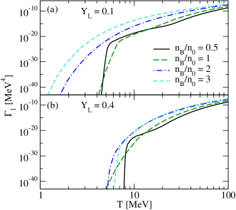
Figure 13: The neutron decay rate $\Gamma_{1}$ as a function of the temperature for fixed values of the baryon density. The lepton fraction is fixed at $Y_{L}=0.1$ for (a) and at $Y_{L}=0.4$ for (b).

In this appendix we discuss the numerical results for the $\beta$-equilibration rates $\Gamma_{1}$ and $\Gamma_{2}$ given by Eqs. (14) and (23). Figures 13 and 14 show the temperature dependence of the neutron decay and the electron capture rates, respectively, for various values of the density and lepton fraction.

Figures 13 and 14 demonstrate that the electron capture process and its inverse (2) dominate the beta equilibration and hence the bulk viscosity. The electron capture rate $\Gamma_{2}$ is always many orders of magnitude larger than the neutron decay rate $\Gamma_{1}$. This is because we are studying neutrino-trapped matter, where the trapped species is typically neutrinos rather than antineutrinos (Figs. 1, 2) so any process involving antineutrinos will be suppressed by factors of $\exp(-\mu{{}_{\nu}}/T)$.

As seen from the upper panels of the figures, $\Gamma_{1}$ is a rapidly increasing function of the temperature and exponentially vanishes at low temperatures because of vanishing antineutrino density in the degenerate matter. The threshold of temperature below which $\Gamma_{1}$ practically vanishes is located at higher temperatures for higher lepton fractions, because the suppression of the antineutrino density is stronger for larger $Y_{L}$.

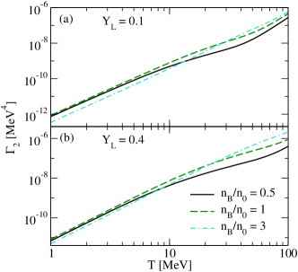
Figure 14: The electron capture rate $\Gamma_{2}$ as a function of the temperature for fixed values of the baryon density. The lepton fraction is fixed at $Y_{L}=0.1$ for (a) and at $Y_{L}=0.4$ for (b).

The temperature dependence of the electron capture rate differs significantly from that of $\Gamma_{1}$. Indeed, $\Gamma_{2}$ increases with the temperature according to a power-law $\Gamma_{2}\propto T^{3}$ up to the temperatures $T\simeq 10$ MeV, as seen from the low-temperature limit given by Eq. (24). This scaling breaks down at higher temperatures $T\geq 10$ MeV and sufficiently low densities $n_{B}\leq n_{0}$, where the finite temperature effects become important in the evaluation of the integral (23). We have checked numerically that the exact result for $\Gamma_{2}$ (23) tends to its low-temperature limit (24) as $T\leq 1$ MeV.

Comparing the upper and lower panels in Figs. 13 and 14, we see that $\Gamma_{1}$ is smaller for larger lepton fraction, whereas $\Gamma_{2}$ shows the opposite behavior. The reason for this behavior is clear: the neutron decay rate $\Gamma_{1}$ is proportional to the antineutrino (number) density, whereas the electron capture rate $\Gamma_{2}$ is proportional to the neutrino density. Because the electron neutrino fraction increases with the increase of $Y_{L}$, as was seen from Figs. 1 and 2, the antineutrino population becomes more suppressed at higher $Y_{L}$, thus leading to smaller $\Gamma_{1}$ and larger $\Gamma_{2}$.

Appendix D Bulk viscosity of neutrino-transparent matter

In this appendix we are interested in the domain of temperatures $T\leq T_{\rm tr}$ where the matter is neutrino transparent ($Y_{\nu}=0$). Below the temperature $T\simeq 1\,{\rm MeV}$, the modified Urca process becomes important Alford:2018lhf therefore our results are strictly relevant for the temperature domain $1\leq T\leq 5$ MeV. To account for uncertainty in the value of $T_{\rm tr}$ the numerical results will be shown up to $T=10$ MeV. The particle fractions are shown in Fig. 15. In this case muons appear only above a certain baryon density $n_{B}\gtrsim n_{0}$, where the condition $\mu_{e}\geq m_{\mu}\simeq 106$ MeV is satisfied. Below this threshold, the proton and electron fractions are equal, as required by the charge neutrality condition, whereas above the threshold the condition $Y_{p}=Y_{e}+Y_{\mu}$ is satisfied.

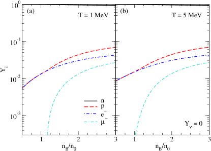
Figure 15: Particle fractions as functions of the baryon density for neutrino-transparent matter $Y_{\nu}=0$ for two values of the temperature: (a) $T=1$ MeV; (b) $T=5$ MeV.

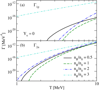
Figure 16: The neutron decay rate $\Gamma_{1p}$ (a) and the electron capture rate $\Gamma_{2n}$ (b) as functions of the temperature for fixed values of the baryon density in the neutrino-transparent case.

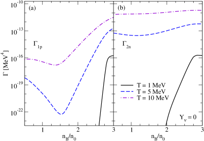
Figure 17: The neutron decay rate $\Gamma_{1p}$ (a) and the electron capture rate $\Gamma_{2n}$ (b) as functions of the baryon density for fixed values of the temperature in the neutrino-transparent case $Y_{\nu}=0$.

The relevant $\beta$-equilibration rates $\Gamma_{1p}$ and $\Gamma_{2n}$ are shown in Fig. 16 and as functions of the temperature. Both quantities rapidly increase with the temperature and are exponentially damped in the low-temperature limit. The reason is that the condition $p_{Fp}+p_{Fe}\geq p_{Fn}$ is never satisfied for the given model of hadronic matter because of very small proton fraction $Y_{p}\leq 7$ %, see Fig. 15. As a consequence, the direct Urca processes for neutrino-transparent matter are always blocked at low temperatures, therefore in that regime, the modified Urca processes should be accurately taken into account Alford:2018lhf .

Quantitatively, the neutron decay rate $\Gamma_{1p}$ in the case of $Y_{\nu}=0$ is larger than in the case of $Y_{L}=0.1$, whereas the electron capture rate is smaller. This result can be anticipated from Eqs. (14) and (23), where one should substitute $\alpha_{\nu}=0$ in the neutrino-transparent case. However, the rate $\Gamma_{1p}$ again remains much smaller than $\Gamma_{2n}$, and only at sufficiently high densities approaches $\Gamma_{2n}$, as seen in Fig. 17, since both quantities have the same low-temperature limit given by Eqs. (16) and (26).

We remark also, that the behavior of $\lambda_{1}$ and $\lambda_{2}$ is very similar to that of $\Gamma_{1p}$ and $\Gamma_{2n}$, respectively. At densities $n_{B}\geq n_{0}$ we have approximately $\lambda_{1}\simeq\Gamma_{1p}/T$ and $\lambda_{2}\simeq\Gamma_{2n}/T$, as it was the case of neutrino-trapped matter, see Eqs. (13) and (22).

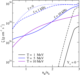
Figure 18: The density dependence of the bulk viscosity for various values of the temperature and the oscillation frequency in the case of $Y_{\nu}=0$. In the case of high temperatures (the violet curve) $\zeta$ becomes independent of the frequency.

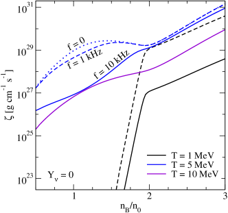
Figure 19: Same as Fig. 18, but for model NL3.

Next, we show the density dependence of the bulk viscosity in Fig. 18. As in the case of $Y_{\nu}\neq 0$, the frequency dependence of $\zeta$ can be neglected at sufficiently high temperatures $T\simeq 10$ MeV (see Fig. 7), and, because the product $\lambda A$ is almost density-independent, the bulk viscosity as a function of density increases as $C^{2}$. For smaller temperatures $T\lesssim 5$ MeV the frequency dependence of $\zeta$ becomes important, and the bulk viscosity drops rapidly with $\omega$. We show the bulk viscosity for three values of the frequency in Fig. 18 for $T=5$ MeV. The general increase of $\zeta$ with the density, in this case, is again caused by the factor $C^{2}$, but the hump structures of $\zeta$ in the range arise from the weak density-dependence of the product $\lambda A$. In the case of $T=1$ MeV we have already the opposite limit $\omega\gg\lambda A$ (see Fig. 7), therefore the bulk viscosity scales as $\zeta\propto\lambda C^{2}$, which rapidly increases with the density and drops to zero at sufficiently low densities $n_{B}\lesssim 2n_{0}$. We have checked that our low-temperature result for $T=0.1$ MeV agrees with the result of the bulk viscosity shown in Fig. 2 of Ref. Haensel2000 obtained for direct Urca processes for the same state of hadronic matter.

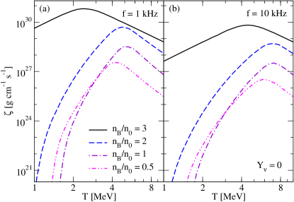
Figure 20: The temperature dependence of the bulk viscosity for model DD-ME2 for various values of the density in the case of $Y_{\nu}=0$. The oscillation frequency is fixed at (a) $f=1$ kHz and (b) $f=10$ kHz.

For comparison, we show also the bulk viscosity of the neutrino-transparent matter for the nuclear model NL3 in Fig. 19. The results obtained within two models DD-ME2 and NL3 differ mainly in the low-temperature region, where the bulk viscosity is strongly suppressed at low densities because of blocking of direct Urca processes. The suppression sets in at lower densities in the case of the NL3 model because this model predicts larger proton and electron fractions than the DD-ME2 model.

Figures 20 and 21 show the temperature dependence of the bulk viscosity for models DD-ME2 and NL3, respectively. It has a maximum at the temperature where $\omega=\lambda A$, and the slope of the curve on the right side of the maximum is larger than in the case of $Y_{\nu}\neq 0$ because of stronger $\lambda=\lambda(T)$ dependence. Using the approximate scaling $\lambda\propto T^{4}$, we find that $T_{\rm max}=(\omega/\lambda_{0}A)^{1/4}$, where $\lambda_{0}$ is the value of $\lambda(T)$ at $T=1$ MeV, i.e., the maximum shifts to higher temperatures for higher frequencies. As seen from a comparison of Figs. 8 and 9 with Figs. 18 and 20, the bulk viscosity is larger in the case of neutrino-transparent matter, as expected.

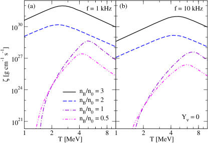
Figure 21: Same as Fig. 20, but for model NL3.

We also compare our results with the high-frequency (low-temperature) result of Ref. Haensel1992PhRvD obtained from direct Urca processes for the neutrino-transparent matter. Choosing the parameters, e.g., $T=1$ MeV, $f=1$ kHz, $n_{B}=2\,n_{0}$, we find from Figs. 1 and 2 and Eq. (13) of Ref. Haensel1992PhRvD the values $\zeta\simeq 3.5\cdot 10^{28}$ g cm^-1 s^-1 for the model I, and $\zeta\simeq 10^{29}$ g cm^-1 s^-1 for model II, whereas our calculations give much lower result $\zeta\simeq 10^{21}$ g cm^-1 s^-1. The reason for this is the lower proton fraction in our model, which leads to blocking of direct Urca processes at low temperatures and, therefore, to lower bulk viscosity.

References

- (1) LIGO Scientific Collaboration and Virgo Collaboration collaboration, The LIGO Scientific Collaboration and The Virgo Collaboration, Gw170817: Observation of gravitational waves from a binary neutron star inspiral, Phys. Rev. Lett. 119 (2017) 161101.
- (2) A. Perego, S. Bernuzzi and D. Radice, Thermodynamics conditions of matter in neutron star mergers, 1903.07898.
- (3) M. Hanauske, J. Steinheimer, A. Motornenko, V. Vovchenko, L. Bovard, E. R. Most et al., Neutron Star Mergers: Probing the EoS of Hot, Dense Matter by Gravitational Waves, Particles 2 (2019) 44–56.
- (4) M. Hanauske, J. Steinheimer, L. Bovard, A. Mukherjee, S. Schramm, K. Takami et al., Concluding Remarks: Connecting Relativistic Heavy Ion Collisions and Neutron Star Mergers by the Equation of State of Dense Hadron- and Quark Matter as signalled by Gravitational Waves, J. Phys. Conf. Ser. 878 (2017) 012031.
- (5) W. Kastaun, R. Ciolfi, A. Endrizzi and B. Giacomazzo, Structure of Stable Binary Neutron Star Merger Remnants: Role of Initial Spin, Phys. Rev. D96 (2017) 043019, [1612.03671].
- (6) S. Bernuzzi, D. Radice, C. D. Ott, L. F. Roberts, P. Moesta and F. Galeazzi, How loud are neutron star mergers?, Phys. Rev. D94 (2016) 024023, [1512.06397].
- (7) F. Foucart, R. Haas, M. D. Duez, E. O’Connor, C. D. Ott, L. Roberts et al., Low mass binary neutron star mergers : gravitational waves and neutrino emission, Phys. Rev. D93 (2016) 044019, [1510.06398].
- (8) K. Kiuchi, Y. Sekiguchi, K. Kyutoku and M. Shibata, Gravitational waves, neutrino emissions, and effects of hyperons in binary neutron star mergers, Class. Quant. Grav. 29 (2012) 124003, [1206.0509].
- (9) Y. Sekiguchi, K. Kiuchi, K. Kyutoku and M. Shibata, Gravitational waves and neutrino emission from the merger of binary neutron stars, Phys. Rev. Lett. 107 (2011) 051102, [1105.2125].
- (10) M. Ruiz, R. N. Lang, V. Paschalidis and S. L. Shapiro, Binary Neutron Star Mergers: A Jet Engine for Short Gamma-Ray Bursts, ApJ Lett. 824 (2016) L6, [1604.02455].
- (11) W. E. East, V. Paschalidis, F. Pretorius and S. L. Shapiro, Relativistic simulations of eccentric binary neutron star mergers: One-arm spiral instability and effects of neutron star spin, Phys. Rev. D 93 (2016) 024011, [1511.01093].
- (12) E. R. Most, L. J. Papenfort, V. Dexheimer, M. Hanauske, S. Schramm, H. Stöcker et al., Signatures of Quark-Hadron Phase Transitions in General-Relativistic Neutron-Star Mergers, Phys. Rev. Lett. 122 (2019) 061101, [1807.03684].
- (13) A. Bauswein, N.-U. F. Bastian, D. B. Blaschke, K. Chatziioannou, J. A. Clark, T. Fischer et al., Identifying a First-Order Phase Transition in Neutron-Star Mergers through Gravitational Waves, Phys. Rev. Lett. 122 (2019) 061102, [1809.01116].
- (14) L. Baiotti and L. Rezzolla, Binary neutron star mergers: a review of Einstein’s richest laboratory, Rept. Prog. Phys. 80 (2017) 096901, [1607.03540].
- (15) J. A. Faber and F. A. Rasio, Binary neutron star mergers, Living Rev. Relativity 15 (2012) .
- (16) M. G. Alford, L. Bovard, M. Hanauske, L. Rezzolla and K. Schwenzer, Viscous Dissipation and Heat Conduction in Binary Neutron-Star Mergers, Physical Review Letters 120 (2018) 041101, [1707.09475].
- (17) A. Harutyunyan and A. Sedrakian, Electrical conductivity of a warm neutron star crust in magnetic fields, Phys. Rev. C 94 (2016) 025805, [1605.07612].
- (18) A. Harutyunyan, A. Nathanail, L. Rezzolla and A. Sedrakian, Electrical resistivity and Hall effect in binary neutron star mergers, European Physical Journal A 54 (2018) 191, [1803.09215].
- (19) L. F. Roberts, S. Reddy and G. Shen, Medium modification of the charged current neutrino opacity and its implications, Phys. Rev. C86 (2012) 065803, [1205.4066].
- (20) M. G. Alford and S. P. Harris, Beta equilibrium in neutron star mergers, Phys. Rev. C98 (2018) 065806, [1803.00662].
- (21) R. F. Sawyer and A. Soni, Transport of neutrinos in hot neutron-star matter, Astrophys. J. 230 (1979) 859–869.
- (22) R. F. Sawyer, Damping of neutron star pulsations by weak interaction processes, Astrophys. J. 237 (1980) 187–197.
- (23) R. F. Sawyer, Bulk viscosity of hot neutron-star matter and the maximum rotation rates of neutron stars, Phys. Rev. D 39 (1989) 3804–3806.
- (24) P. Haensel and R. Schaeffer, Bulk viscosity of hot-neutron-star matter from direct URCA processes, Phys. Rev. D 45 (1992) 4708–4712.
- (25) H. Dong, N. Su and Q. Wang, Bulk viscosity in nuclear and quark matter, Journal of Physics G Nuclear Physics 34 (2007) S643–S646, [astro-ph/0702181].
- (26) M. G. Alford, S. Mahmoodifar and K. Schwenzer, Large amplitude behavior of the bulk viscosity of dense matter, Journal of Physics G Nuclear Physics 37 (2010) 125202, [1005.3769].
- (27) E. E. Kolomeitsev and D. N. Voskresensky, Viscosity of neutron star matter and r -modes in rotating pulsars, Phys. Rev. C 91 (2015) 025805, [1412.0314].
- (28) M. G. Alford and G. Good, Leptonic contribution to the bulk viscosity of nuclear matter, Phys. Rev. C82 (2010) 055805, [1003.1093].
- (29) P. B. Jones, Bulk viscosity of neutron-star matter, Phys. Rev. D 64 (2001) 084003.
- (30) L. Lindblom and B. J. Owen, Effect of hyperon bulk viscosity on neutron-star r-modes, Phys. Rev. D 65 (2002) 063006, [astro-ph/0110558].
- (31) E. N. van Dalen and A. E. Dieperink, Bulk viscosity in neutron stars from hyperons, Phys. Rev. C 69 (2004) 025802, [nucl-th/0311103].
- (32) P. Haensel, K. P. Levenfish and D. G. Yakovlev, Bulk viscosity in superfluid neutron star cores. III. Effects of hyperons, Astron.& Astrophys. 381 (2002) 1080–1089, [astro-ph/0110575].
- (33) D. Chatterjee and D. Bandyopadhyay, Effect of hyperon-hyperon interaction on bulk viscosity and r-mode instability in neutron stars, Phys. Rev. D 74 (2006) 023003, [astro-ph/0602538].
- (34) D. Chatterjee and D. Bandyopadhyay, Hyperon Bulk Viscosity in the Presence of Antikaon Condensate, Astrophys. J. 680 (2008) 686–694, [0712.3171].
- (35) J. Madsen, Bulk viscosity of strange quark matter, damping of quark star vibration, and the maximum rotation rate of pulsars, Phys. Rev. D 46 (1992) 3290–3295.
- (36) A. Drago, A. Lavagno and G. Pagliara, Bulk viscosity in hybrid stars, Phys. Rev. D 71 (2005) 103004, [astro-ph/0312009].
- (37) M. G. Alford and A. Schmitt, Bulk viscosity in 2SC quark matter, J. Phys. G34 (2007) 67–102, [nucl-th/0608019].
- (38) M. G. Alford, M. Braby, S. Reddy and T. Schäfer, Bulk viscosity due to kaons in color-flavor-locked quark matter, Phys. Rev. C75 (2007) 055209, [nucl-th/0701067].
- (39) C. Manuel and F. J. Llanes-Estrada, Bulk viscosity in a cold CFL superfluid, JCAP 0708 (2007) 001, [0705.3909].
- (40) B. A. Sa’d, I. A. Shovkovy and D. H. Rischke, Bulk viscosity of strange quark matter: Urca versus nonleptonic processes, Phys. Rev. D 75 (2007) 125004, [astro-ph/0703016].
- (41) B. A. Sa’d, I. A. Shovkovy and D. H. Rischke, Bulk viscosity of spin-one color superconductors with two quark flavors, Phys. Rev. D 75 (2007) 065016, [astro-ph/0607643].
- (42) M. G. Alford, M. Braby and A. Schmitt, Bulk viscosity in kaon-condensed color-flavor locked quark matter, J. Phys. G35 (2008) 115007, [0806.0285].
- (43) M. Sinha and D. Bandyopadhyay, Hyperon bulk viscosity in strong magnetic fields, Phys. Rev. D 79 (2009) 123001, [0809.3337].
- (44) X. Wang and I. A. Shovkovy, Bulk viscosity of spin-one color superconducting strange quark matter, Phys. Rev. D 82 (2010) 085007, [1006.1293].
- (45) X.-G. Huang, M. Huang, D. H. Rischke and A. Sedrakian, Anisotropic hydrodynamics, bulk viscosities, and r-modes of strange quark stars with strong magnetic fields, Phys. Rev. D 81 (2010) 045015, [0910.3633].
- (46) M. G. Alford, S. Han and K. Schwenzer, Phase conversion dissipation in multicomponent compact stars, Phys. Rev. C 91 (2015) 055804, [1404.5279].
- (47) A. Schmitt and P. Shternin, Reaction rates and transport in neutron stars, ArXiv e-prints (2017) , [1711.06520].
- (48) P. Haensel, K. P. Levenfish and D. G. Yakovlev, Bulk viscosity in superfluid neutron star cores. I. Direct Urca processes in npemu matter, Astron.& Astrophys. 357 (2000) 1157–1169, [astro-ph/0004183].
- (49) P. Haensel, K. P. Levenfish and D. G. Yakovlev, Bulk viscosity in superfluid neutron star cores. II. Modified Urca processes in npe mu matter, Astron.& Astrophys. 372 (2001) 130–137, [astro-ph/0103290].
- (50) M. E. Gusakov, Bulk viscosity of superfluid neutron stars, Phys. Rev. D 76 (2007) 083001, [0704.1071].
- (51) W. Greiner and B. Müller, Gauge Theory of Weak Interactions. Physics and Astronomy Online Library. Springer, 2000.
- (52) N. Glendenning, Compact Stars: Nuclear Physics, Particle Physics, and General Relativity. Astronomy and Astrophysics Library. Springer New York, 2000.
- (53) F. Weber, Pulsars as astrophysical laboratories for nuclear and particle physics. Institute of Physics, Bristol, U.K., 1999.
- (54) A. Sedrakian, The physics of dense hadronic matter and compact stars, Prog. Part. Nucl. Phys. 58 (2007) 168–246.
- (55) G. A. Lalazissis, T. Nikšić, D. Vretenar and P. Ring, New relativistic mean-field interaction with density-dependent meson-nucleon couplings, Phys. Rev. C 71 (2005) 024312.
- (56) G. Colucci and A. Sedrakian, Equation of state of hypernuclear matter: Impact of hyperon-scalar-meson couplings, Phys. Rev. C 87 (2013) 055806, [1302.6925].
- (57) G. A. Lalazissis, J. König and P. Ring, New parametrization for the Lagrangian density of relativistic mean field theory, Phys. Rev. C 55 (Jan, 1997) 540–543, [nucl-th/9607039].
- (58) M. Prakash, I. Bombaci, M. Prakash, P. J. Ellis, J. M. Lattimer and R. Knorren, Composition and structure of protoneutron stars, Physics Reports 280 (Jan, 1997) 1–77, [nucl-th/9603042].
- (59) G. Malfatti, M. G. Orsaria, G. A. Contrera, F. Weber and I. F. Ranea-Sand oval, Hot quark matter and (proto-) neutron stars, Physical Review C 100 (Jul, 2019) 015803, [1907.06597].
- (60) F. Weber, D. Farrell, W. M. Spinella, G. Malfatti, M. G. Orsaria, G. A. Contrera et al., Phases of Hadron-Quark Matter in (Proto) Neutron Stars, Universe 5 (Jul, 2019) 169, [1907.06591].
- (61) M. Alford and S. Harris, Damping of density oscillations in neutrino-transparent nuclear matter, Phys. Rev. C 100 (2019) 035803, [1907.03795].
- (62) D. G. Yakovlev, M. E. Gusakov and P. Haensel, Bulk viscosity in a neutron star mantle, Mon. Not. RAS 481 (2018) 4924–4930, [1809.08609].
- (63) J. J. Li, A. Sedrakian and F. Weber, Competition between delta isobars and hyperons and properties of compact stars, Phys. Lett. B 783 (2018) 234–240, [1803.03661].
- (64) J. J. Li and A. Sedrakian, Implications from GW170817 for -isobar Admixed Hypernuclear Compact Stars, ApJ Lett. 874 (2019) L22, [1904.02006].
- (65) D. Chatterjee and D. Bandyopadhyay, Bulk viscosity in kaon condensed matter, Phys. Rev. D 75 (Jun, 2007) 123006, [astro-ph/0702259].