Resource theory of entanglement for bipartite quantum channels

Abstract

The traditional perspective in quantum resource theories concerns how to use free operations to convert one resourceful quantum state to another one. For example, a fundamental and well known question in entanglement theory is to determine the distillable entanglement of a bipartite state, which is equal to the maximum rate at which fresh Bell states can be distilled from many copies of a given bipartite state by employing local operations and classical communication for free. It is the aim of this paper to take this kind of question to the next level, with the main question being: What is the best way of using free channels to convert one resourceful quantum channel to another? Here we focus on the the resource theory of entanglement for bipartite channels and establish several fundamental tasks and results regarding it. In particular, we establish bounds on several pertinent information processing tasks in channel entanglement theory, and we define several entanglement measures for bipartite channels, including the logarithmic negativity and the $\kappa$-entanglement. We also show that the max-Rains information of [Bäuml et al., Physical Review Letters, 121, 250504 (2018)] has a divergence interpretation, which is helpful for simplifying the results of this earlier work.

1 Introduction

Ever since the development of the resource theory of entanglement [BDSW96, HHHH09], the investigation of quantum resource theories has blossomed [HO13, Fri15, KdR16, dRKR17, CG18]. This is due to such a framework being a powerful conceptual approach for understanding physical processes, while also providing the ability to apply tools developed in one domain to another. Any given resource theory is specified by a set of free quantum states, as well as a set of restricted free operations, which output a free state when the input is a free state [HO13, CG18].

In the well known example of the resource theory of entanglement [BDSW96, HHHH09], the free states are the separable, unentangled states and the free operations consist of local operations and classical communication (LOCC). One early insight in quantum information theory was to modify the resource theory of entanglement to become the resource theory of non-positive partial transpose states [Rai99, Rai01], by enlarging the set of free states to consist of the positive partial transpose (PPT) states and the class of free operations to consist of those that preserve the PPT states. Consequently, it is then possible to use this modified resource theory to deepen our understanding of the resource theory of entanglement. Inspired by this approach, the resource theory of $k$-unextendibility was recently developed, and this consistent framework ended up giving tighter bounds on non-asymptotic rates of quantum communication [KDWW18].

The traditional approach to research on quantum resource theories is to address the following fundamental question: In a given resource theory, what is the best way to use a free quantum channel to convert one quantum state to another? For concreteness, consider the well known resource theory of entanglement. There, one asks about using an LOCC channel to convert from one bipartite quantum state $\rho_{AB}$ to another bipartite state $\sigma_{AB}$. First, is the transition possible? Next, what is the best asymptotic rate $R$ at which it is possible to start from $nR$ independent copies of $\rho_{AB}$ and convert them approximately or exactly by LOCC to $n$ independent copies of $\sigma_{AB}$? Is the resource theory reversible, in the sense that one could start from $nR$ copies of $\rho_{AB}$, convert by LOCC to $n$ copies of $\sigma_{AB}$, and then convert back to $nR$ copies of $\rho_{AB}$? These kinds of questions have been effectively addressed in a number of different works on quantum information theory [BDSW96, BBPS96, Nie99, Rai99, Rai01, HHT01, BP08, KH13, WD16a, WD17a], and the earlier works can in fact be considered the starting point for the modern approach to quantum resource theories.

However, upon seeing the above questions, one might have a basic question that is not addressed by the above framework: How is the initial bipartite state $\rho_{AB}$ created in the first place? That is, how is it that two parties, Alice and Bob, are able to share such a state between their distant laboratories? It is of course necessary that they employ a communication medium, such as a fiber-optic cable or a free space link modeled as a quantum channel, in order to do so. A model for the communication medium is given by a bipartite quantum channel [BHLS03, CLL06], which is a four-terminal device consisting of two inputs and two outputs, with one input and one output for Alice and one input and one output for Bob. The basic question above motivates developing the resource theory of entanglement for bipartite quantum channels, and the main thrust of this paper is to do so. The paper [BHLS03] initiated this direction, but there are a large number of questions that have remained unaddressed, and now we have a number of tools and conceptual approachs to address these fundamental questions [BBCW13, BW18, DBW17, BDW18, Das18, Wil18a, WW18].

Thus, the motivation for this new direction is that quantum processes (channels) are more fundamental than quantum states, in the sense that quantum states can only arise from quantum processes, and so we should shift the focus to quantifying the resourcefulness of a quantum channel. In fact, every basic constituent of quantum mechanics, including states, unitaries, measurements, and discarding of quantum systems are particular kinds of quantum channels. In this way, a general goal is to develop complete resource theories of quantum channels [LY19, LW19], and the outcome will be a more complete understanding of entanglement, purity, magic, coherence, distinguishability, etc. [BHLS03, BDGDMW17, DBW17, GFW⁺18, BDW18, Das18, TEZP19, WW18, SC19, WWS19, LY19, LW19, WW19].

Specifically, in the context of the resource theory of entanglement for bipartite quantum channels, the main question that we are interested in addressing is this: Given $n$ independent uses of a bipartite quantum channel $\mathcal{N}_{A^{\prime}B^{\prime}\rightarrow AB}$ with input quantum systems $A^{\prime}$ and $B^{\prime}$ and output systems $A$ and $B$, as well as free LOCC, what is the best asymptotic rate $R$ that one can achieve for a faithful simulation of $nR$ independent uses of another bipartite quantum channel $\mathcal{M}_{\hat{A}^{\prime}\hat{B}^{\prime}\rightarrow\hat{A}\hat{B}}$ with input systems $\hat{A}^{\prime}$ and $\hat{B}^{\prime}$ and output systems $\hat{A}$ and $\hat{B}$, in the limit of large $n$? Furthermore, we are interested in the most general notion of channel simulation introduced recently in [Wil18a], in which the simulated channel uses can be called in a sequential manner, by the most general verifier who can act sequentially. Note that prior work on channel simulation [BDH⁺14, BCR11, BBCW13] only considered a particular notion of channel simulation, as well as a particular kind of channel to be simulated, in which the goal is to simulate $nR$ independent parallel uses of a point-to-point channel $\mathcal{P}_{A\rightarrow B}$. Also, the traditional resource theory of entanglement for states emerges as a special case of this more general resource theory, for the case in which the bipartite channel simply traces out the inputs of Alice and Bob and replaces them with some bipartite state $\rho_{AB}$.

There are certainly interesting special cases of the aforementioned general question, which already would take us beyond what is currently known: How much entanglement can be distilled from $n$ independent uses of a bipartite channel $\mathcal{N}_{A^{\prime}B^{\prime}\rightarrow AB}$ assisted by free LOCC? How much entanglement is required to simulate $nR$ independent uses of a bipartite channel $\mathcal{M}_{\hat{A}^{\prime}\hat{B}^{\prime}\rightarrow\hat{A}\hat{B}}$, such that the most stringest verifier, who performs a sequential test, cannot distinguish the actual channel uses from the simulation? What if the distillation or simulation is required to be approximate or exact? How do the rates change? How does the theory change if we allow completely PPT-preserving channels for free, as Rains [Rai99, Rai01] did? What if we allow the $k$-extendible channels of [KDWW18] for free instead?

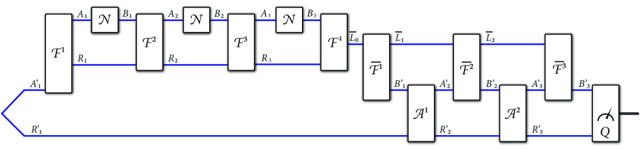
Figure 1: The figure displays a protocol that consumes three uses of a quantum channel $\mathcal{N}_{A\to B}$ to simulate three uses of another quantum channel $\mathcal{M}_{A^{\prime}\to B^{\prime}}$. Channels labeled as $\mathcal{F}$ are free in some given resource theory and can thus be consumed at no cost. The simulation should be such that any discriminator employing an initial state on systems $R_{1}^{\prime}A_{1}^{\prime}$, along with adaptive channels $\mathcal{A}^{1}$ and $\mathcal{A}^{2}$ and a final measurement $Q$ on systems $R_{3}^{\prime}B_{3}^{\prime}$, cannot distinguish the simulation from three uses of $\mathcal{M}_{A^{\prime}\to B^{\prime}}$.

More generally, one can address these questions in general quantum resource theories. This constitutes a fundamental rethinking and generalization of all of the recent work on quantum resource theories. The basic question phrased above then becomes as follows: In a given resource theory, if $n$ independent uses of a resourceful quantum channel $\mathcal{N}$ are available, along with the assistance of free operations, what is the maximum possible rate $R$ at which one can simulate $nR$ independent uses of another resourceful channel $\mathcal{M}$? Figure 1 depicts a general protocol that can accomplish this task in any resource theory.

For the rest of the paper, we begin by giving some background in the next section. We then frame the aforementioned fundamental questions in more detail and offer solutions in some cases. The next part of the paper then proposes some entanglement measures for bipartite channels, including the logarithmic negativity, the $\kappa$-entanglement, and the generalized Rains information. We establish several fundamental properties of these measures.

Note on related work: Recently and independently of us, the resource theory of entanglement for bipartite channels was considered in [GS19]. The paper [GS19] also defined and considered some fundamental tasks in the theory, in addition to defining entanglement measures for bipartite channels, such as logarithmic negativity and $\kappa$-entanglement.

2 Background: States, channels, isometries, separable states, and positive partial transpose

We begin by establishing some notation and reviewing some definitions needed in the rest of the paper. Let $\mathcal{B}(\mathcal{H})$ denote the algebra of bounded linear operators acting on a Hilbert space $\mathcal{H}$. Throughout this paper, we restrict our development to finite-dimensional Hilbert spaces. The subset of $\mathcal{B}(\mathcal{H})$ containing all positive semi-definite operators is denoted by $\mathcal{B}_{+}(\mathcal{H})$. We denote the identity operator as $I$ and the identity superoperator as $\operatorname{id}$. The Hilbert space of a quantum system $A$ is denoted by $\mathcal{H}_{A}$. The state of a quantum system $A$ is represented by a density operator $\rho_{A}$, which is a positive semi-definite operator with unit trace. Let $\mathcal{D}(\mathcal{H}_{A})$ denote the set of density operators, i.e., all elements $\rho_{A}\in\mathcal{B}_{+}(\mathcal{H}_{A})$ such that $\operatorname{Tr}\{\rho_{A}\}=1$. The Hilbert space for a composite system $LA$ is denoted as $\mathcal{H}_{LA}$ where $\mathcal{H}_{LA}=\mathcal{H}_{L}\otimes\mathcal{H}_{A}$. The density operator of a composite system $LA$ is defined as $\rho_{LA}\in\mathcal{D}(\mathcal{H}_{LA})$, and the partial trace over $A$ gives the reduced density operator for system $L$, i.e., $\operatorname{Tr}_{A}\{\rho_{LA}\}=\rho_{L}$ such that $\rho_{L}\in\mathcal{D}(\mathcal{H}_{L})$. The notation $A^{n}:=A_{1}A_{2}\cdots A_{n}$ indicates a composite system consisting of $n$ subsystems, each of which is isomorphic to the Hilbert space $\mathcal{H}_{A}$. A pure state $\psi_{A}$ of a system $A$ is a rank-one density operator, and we write it as $\psi_{A}=|\psi\rangle\langle\psi|_{A}$ for $|\psi\rangle_{A}$ a unit vector in $\mathcal{H}_{A}$. A purification of a density operator $\rho_{A}$ is a pure state $\psi^{\rho}_{EA}$ such that $\operatorname{Tr}_{E}\{\psi^{\rho}_{EA}\}=\rho_{A}$, where $E$ is called the purifying system. The maximally mixed state is denoted by $\pi_{A}:=I_{A}/\dim(\mathcal{H}_{A})\in\mathcal{D}\left(\mathcal{H}_{A}\right)$. The fidelity of $\tau,\sigma\in\mathcal{B}_{+}(\mathcal{H})$ is defined as $F(\tau,\sigma)=\left\|{\sqrt{\tau}\sqrt{\sigma}}\right\|_{1}^{2}$ [Uhl76], with the trace norm $\left\|{X}\right\|_{1}=\operatorname{Tr}\sqrt{X^{\dagger}X}$ for $X\in\mathcal{B}(\mathcal{H})$.

The adjoint $\mathcal{M}^{\dagger}:\mathcal{B}(\mathcal{H}_{B})\to\mathcal{B}(\mathcal{H}_{A})$ of a linear map $\mathcal{M}:\mathcal{B}(\mathcal{H}_{A})\to\mathcal{B}(\mathcal{H}_{B})$ is the unique linear map such that

$$\langle Y_{B},\mathcal{M}(X_{A})\rangle=\langle\mathcal{M}^{\dagger}(Y_{B}),X_{A}\rangle,$$ (2.1)

for all $X_{A}\in\mathcal{B}(\mathcal{H}_{A})$ and $Y_{B}\in\mathcal{B}(\mathcal{H}_{B})$, where $\langle C,D\rangle=\operatorname{Tr}\{C^{\dagger}D\}$ is the Hilbert-Schmidt inner product. An isometry $U:\mathcal{H}\to\mathcal{H}^{\prime}$ is a linear map such that $U^{{\dagger}}U=I_{\mathcal{H}}$.

The evolution of a quantum state is described by a quantum channel. A quantum channel $\mathcal{M}_{A\to B}$ is a completely positive, trace-preserving (CPTP) map $\mathcal{M}:\mathcal{B}_{+}(\mathcal{H}_{A})\to\mathcal{B}_{+}(\mathcal{H}_{B})$.

Let $U^{\mathcal{M}}_{A\to BE}$ denote an isometric extension of a quantum channel $\mathcal{M}_{A\to B}$, which by definition means that for all $\rho_{A}\in\mathcal{D}\left(\mathcal{H}_{A}\right)$,

$$\operatorname{Tr}_{E}\left\{U^{\mathcal{M}}_{A\to BE}\rho_{A}\left(U^{\mathcal{M}}_{A\to BE}\right)^{\dagger}\right\}=\mathcal{M}_{A\to B}(\rho_{A}),$$ (2.2)

along with the following conditions for $U^{\mathcal{M}}$ to be an isometry:

$$(U^{\mathcal{M}})^{\dagger}U^{\mathcal{M}}=I_{A}.$$ (2.3)

Hence $U^{\mathcal{M}}(U^{\mathcal{M}})^{\dagger}=\Pi_{BE}$, where $\Pi_{BE}$ is a projection onto a subspace of the Hilbert space $\mathcal{H}_{BE}$. A complementary channel $\widehat{\mathcal{M}}_{A\to E}$ of $\mathcal{M}_{A\to B}$ is defined as

$$\widehat{\mathcal{M}}_{A\to E}(\rho_{A}):=\operatorname{Tr}_{B}\left\{U^{\mathcal{M}}_{A\to BE}\rho_{A}(U^{\mathcal{M}}_{A\to BE})^{\dagger}\right\},$$ (2.4)

for all $\rho_{A}\in\mathcal{D}\left(\mathcal{H}_{A}\right)$.

The Choi isomorphism represents a well known duality between channels and states. Let $\mathcal{M}_{A\to B}$ be a quantum channel, and let $\left|\Upsilon\right>_{L:A}$ denote the following maximally entangled vector:

$$|\Upsilon\rangle_{L:A}\coloneqq\sum_{i}|i\rangle_{L}|i\rangle_{A},$$ (2.5)

where $\dim(\mathcal{H}_{L})=\dim(\mathcal{H}_{A})$, and $\{|i\rangle_{L}\}_{i}$ and $\{|i\rangle_{A}\}_{i}$ are fixed orthonormal bases. We extend this notation to multiple parties with a given bipartite cut as

$$|\Upsilon\rangle_{L_{A}L_{B}:AB}\coloneqq|\Upsilon\rangle_{L_{A}:A}\otimes|\Upsilon\rangle_{L_{B}:B}.$$ (2.6)

The maximally entangled state $\Phi_{LA}$ is denoted as

$$\Phi_{LA}=\frac{1}{|A|}\left|{\Upsilon}\right\rangle\!\left\langle{\Upsilon}\right|_{LA},$$ (2.7)

where $|A|=\dim(\mathcal{H}_{A})$. The Choi operator for a channel $\mathcal{M}_{A\to B}$ is defined as

$$J^{\mathcal{M}}_{LB}=(\operatorname{id}_{L}\otimes\mathcal{M}_{A\to B})\left(|\Upsilon\rangle\langle\Upsilon|_{LA}\right),$$ (2.8)

where $\operatorname{id}_{L}$ denotes the identity map on $L$. For $A^{\prime}\simeq A$, the following identity holds

$$\langle\Upsilon|_{A^{\prime}:L}(\rho_{SA^{\prime}}\otimes J^{\mathcal{M}}_{LB})|\Upsilon\rangle_{A^{\prime}:L}=\mathcal{M}_{A\to B}(\rho_{SA}),$$ (2.9)

where $A^{\prime}\simeq A$. The above identity can be understood in terms of a post-selected variant [HM04] of the quantum teleportation protocol [BBC⁺93]. Another identity that holds is

$$\langle\Upsilon|_{L:A}[Q_{SL}\otimes I_{A}]|\Upsilon\rangle_{L:A}=\operatorname{Tr}_{L}\{Q_{SL}\},$$ (2.10)

for an operator $Q_{SL}\in\mathcal{B}(\mathcal{H}_{S}\otimes\mathcal{H}_{L})$.

For a fixed basis $\{|i\rangle_{B}\}_{i}$, the partial transpose $\operatorname{T}_{B}$ on system $B$ is the following map:

$$\left(\operatorname{id}_{A}\otimes\operatorname{T}_{B}\right)(Q_{AB})=\sum_{i,j}\left(I_{A}\otimes|i\rangle\langle j|_{B}\right)Q_{AB}\left(I_{A}\otimes|i\rangle\langle j|_{B}\right),\,$$ (2.11)

where $Q_{AB}\in\mathcal{B}(\mathcal{H}_{A}\otimes\mathcal{H}_{B})$. Further, it holds that

$$\left(Q_{SL}\otimes I_{A}\right)|\Upsilon\rangle_{L:A}=\left(T_{A}\left(Q_{SA}\right)\otimes I_{L}\right)|\Upsilon\rangle_{L:A}.$$ (2.12)

We note that the partial transpose is self-adjoint, i.e., $\operatorname{T}_{B}=\operatorname{T}^{\dagger}_{B}$ and is also involutory:

$$\operatorname{T}_{B}\circ\operatorname{T}_{B}=I_{B}.$$ (2.13)

The following identity also holds:

$$\operatorname{T}_{L}(\left|{\Upsilon}\right\rangle\!\left\langle{\Upsilon}\right|_{LA})=\operatorname{T}_{A}(\left|{\Upsilon}\right\rangle\!\left\langle{\Upsilon}\right|_{LA})$$ (2.14)

Let $\operatorname{SEP}(A\!:\!B)$ denote the set of all separable states $\sigma_{AB}\in\mathcal{D}(\mathcal{H}_{A}\otimes\mathcal{H}_{B})$, which are states that can be written as

$$\sigma_{AB}=\sum_{x}p(x)\omega^{x}_{A}\otimes\tau^{x}_{B},$$ (2.15)

where $p(x)$ is a probability distribution, $\omega^{x}_{A}\in\mathcal{D}(\mathcal{H}_{A})$, and $\tau^{x}_{B}\in\mathcal{D}(\mathcal{H}_{B})$ for all $x$. This set is closed under the action of the partial transpose maps $\operatorname{T}_{A}$ and $\operatorname{T}_{B}$ [HHH96, Per96]. Generalizing the set of separable states, we can define the set $\operatorname{PPT}(A\!:\!B)$ of all bipartite states $\rho_{AB}$ that remain positive after the action of the partial transpose $\operatorname{T}_{B}$. A state $\rho_{AB}\in\operatorname{PPT}(A\!:\!B)$ is also called a PPT (positive under partial transpose) state. We can define an even more general set of positive semi-definite operators [ADMVW02] as follows:

$$\operatorname{PPT}^{\prime}(A\!:\!B)\coloneqq\{\sigma_{AB}:\ \sigma_{AB}\geq 0\land\left\|{\operatorname{T}_{B}(\sigma_{AB})}\right\|_{1}\leq 1\}.$$ (2.16)

We then have the containments $\operatorname{SEP}\subset\operatorname{PPT}\subset\operatorname{PPT}^{\prime}$. A bipartite quantum channel $\mathcal{P}_{A^{\prime}B^{\prime}\to AB}$ is a completely PPT-preserving channel if the map $\operatorname{T}_{B}\circ\mathcal{P}_{A^{\prime}B^{\prime}\to AB}\circ\operatorname{T}_{B^{\prime}}$ is a quantum channel [Rai99, Rai01, CdVGG17]. A bipartite quantum channel $\mathcal{P}_{A^{\prime}B^{\prime}\to AB}$ is completely PPT-preserving if and only if its Choi state is a PPT state [Rai01], i.e., $\frac{J^{\mathcal{P}}_{L_{A}L_{B}:AB}}{|L_{A}L_{B}|}\in\operatorname{PPT}(L_{A}A\!:\!BL_{B})$, where

$$\frac{J^{\mathcal{P}}_{L_{A}L_{B}:AB}}{|L_{A}L_{B}|}=\mathcal{P}_{A^{\prime}B^{\prime}\to AB}(\Phi_{L_{A}A^{\prime}}\otimes\Phi_{B^{\prime}L_{B}}).$$ (2.17)

Any local operations and classical communication (LOCC) channel is a completely PPT-preserving channel [Rai99, Rai01].

2.1 Channels with symmetry

Consider a finite group $G$. For every $g\in G$, let $g\to U_{A}(g)$ and $g\to V_{B}(g)$ be projective unitary representations of $g$ acting on the input space $\mathcal{H}_{A}$ and the output space $\mathcal{H}_{B}$ of a quantum channel $\mathcal{M}_{A\to B}$, respectively. A quantum channel $\mathcal{M}_{A\to B}$ is covariant with respect to these representations if the following relation is satisfied [Hol02, Hol12]:

$$\mathcal{M}_{A\to B}\!\left(U_{A}(g)\rho_{A}U_{A}^{\dagger}(g)\right)=V_{B}(g)\mathcal{M}_{A\to B}(\rho_{A})V_{B}^{\dagger}(g),$$ (2.18)

for all $\rho_{A}\in\mathcal{D}(\mathcal{H}_{A})$ and $g\in G$.

Definition 1 (Covariant channel [Hol12])

A quantum channel is covariant if it is covariant with respect to a group $G$ which has a representation $U(g)$, for all $g\in G$, on $\mathcal{H}_{A}$ that is a unitary one-design; i.e., the map $\frac{1}{|G|}\sum_{g\in G}U(g)(\cdot)U^{\dagger}(g)$ always outputs the maximally mixed state for all input states.

Definition 2 (Teleportation-simulable [BDSW96, HHH99])

A channel $\mathcal{M}_{A\to B}$ is teleportation-simulable with associated resource state $\omega_{L_{A}B}$ if for all $\rho_{A}\in\mathcal{D}\left(\mathcal{H}_{A}\right)$ there exists a resource state $\omega_{L_{A}B}\in\mathcal{D}\left(\mathcal{H}_{L_{A}B}\right)$ such that

$$\mathcal{M}_{A\to B}\left(\rho_{A}\right)=\mathcal{L}_{L_{A}AB\to B}\left(\rho_{A}\otimes\omega_{L_{A}B}\right),$$ (2.19)

where $\mathcal{L}_{L_{A}AB\to B}$ is an LOCC channel (a particular example of an LOCC channel is a generalized teleportation protocol [Wer01]).

One can find the defining equation (2.19) explicitly stated as [HHH99, Eq. (11)]. All covariant channels, as given in Definition 1, are teleportation-simulable with respect to the resource state $\mathcal{M}_{A\to B}(\Phi_{L_{A}A})$ [CDP09b].

Definition 3 (PPT-simulable [KW17])

A channel $\mathcal{M}_{A\to B}$ is PPT-simulable with associated resource state $\omega_{L_{A}B}$ if for all $\rho_{A}\in\mathcal{D}\left(\mathcal{H}_{A}\right)$ there exists a resource state $\omega_{L_{A}B}\in\mathcal{D}\left(\mathcal{H}_{L_{A}B}\right)$ such that

$$\mathcal{M}_{A\to B}\left(\rho_{A}\right)=\mathcal{P}_{L_{A}AB\to B}\left(\rho_{A}\otimes\omega_{L_{A}B}\right),$$ (2.20)

where $\mathcal{P}_{L_{A}AB\to B}$ is a completely PPT-preserving channel acting on $L_{A}A:B$, where the transposition map is with respect to the system $B$.

We note here that all of the above concepts can be generalized to bipartite channels and are helpful in the resource theory of entanglement for bipartite channels.

3 Resource theory of entanglement for bipartite quantum channels

To begin with, let us consider the basic ideas for the resource theory of entanglement for bipartite channels. Our specific goals are to characterize the approximate and exact entanglement costs of bipartite channels, as well as the approximate and exact distillable entanglement of bipartite channels. We can also take the free operations to be LOCC, separable, completely PPT-preserving, or $k$-extendible. These more basic problems are the basis for the more general question, as raised above, of simulating one bipartite quantum channel using another. Let us also emphasize here that the basic questions posed can be considered in any resource theory, such as magic, purity, thermodynamics, coherence, etc.

3.1 Approximate and sequential entanglement cost of bipartite quantum channels

The first problem to consider is the entanglement cost of a bipartite channel, and we focus first on approximate simulation in the Shannon-theoretic sense. In [Wil18a], a general definition of entanglement cost of a single-sender, single-receiver channel was proposed, and here we extend this notion further to bipartite channels. To this end, let $\mathcal{N}_{A^{\prime}B^{\prime}\rightarrow AB}$ denote a bipartite channel (completely positive, trace-preserving map) with input systems $A^{\prime}$ and $B^{\prime}$ and output systems $A$ and $B$. The goal is to determine the rate at which maximally entangled states are needed to simulate $n$ uses of the bipartite channel $\mathcal{N}_{A^{\prime}B^{\prime}\rightarrow AB}$, such that these $n$ uses could be called sequentially and thus employed in any desired context. As discussed for the case of point-to-point channels in [Wil18a], such a sequential simulation is more general and more difficult to analyze than the prior notions of parallel channel simulation put forward in [BBCW13].

In more detail, let us describe what we mean by the (sequential) entanglement cost of a bipartite channel. Fix $n,M\in\mathbb{N}$, $\varepsilon\in\left[0,1\right]$, and a bipartite quantum channel $\mathcal{N}_{A^{\prime}B^{\prime}\rightarrow AB}$. We define an $(n,M,\varepsilon)$ (sequential) LOCC-assisted channel simulation code to consist of a maximally entangled resource state $\Phi_{\overline{A}_{0}\overline{B}_{0}}$ of Schmidt rank $M$ and a set

$$\{\mathcal{L}_{A_{i}^{\prime}B_{i}^{\prime}\overline{A}_{i-1}\overline{B}_{i-1}\rightarrow A_{i}B_{i}\overline{A}_{i}\overline{B}_{i}}^{(i)}\}_{i=1}^{n}$$ (3.1)

of LOCC channels. Note that the systems $\overline{A}_{n}\overline{B}_{n}$ of the final LOCC channel $\mathcal{L}_{A_{n}^{\prime}B_{n}^{\prime}\overline{A}_{n-1}\overline{B}_{n-1}\rightarrow A_{n}B_{n}\overline{A}_{n}\overline{B}_{n}}^{(n)}$ can be taken trivial without loss of generality. Alice has access to all systems labeled by $A$, Bob has access to all systems labeled by $B$, and they are in distant laboratories. The structure of this simulation protocol is intended to be compatible with a discrimination strategy that can test the actual $n$ channels versus the above simulation in a sequential way, along the lines discussed in [CDP08, CDP09a] and [GW07, Gut12]. This encompasses the parallel discrimination test, along the lines considered in [BBCW13], as a special case.

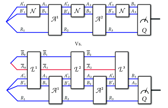
Figure 2: The top part of the figure displays a three-round interaction between the discriminator and the simulator in the case that the actual bipartite channel $\mathcal{N}_{A^{\prime}B^{\prime}\rightarrow AB}$ is called three times. The bottom part of the figure displays the interaction between the discriminator and the simulator in the case that the simulation of three channel uses is called.

A sequential discrimination strategy consists of an initial state $\rho_{R_{1}A_{1}^{\prime}B_{1}^{\prime}}$, a set $\{\mathcal{A}_{R_{i}A_{i}B_{i}\rightarrow R_{i+1}A_{i+1}^{\prime}B_{i+1}^{\prime}}^{(i)}\}_{i=1}^{n-1}$ of adaptive channels, and a quantum measurement $\{Q_{R_{n}A_{n}B_{n}},I_{R_{n}A_{n}B_{n}}-Q_{R_{n}A_{n}B_{n}}\}$. Let the shorthand $\{\rho,\mathcal{A},Q\}$ denote such a discrimination strategy. Note that, in performing a discrimination strategy, the discriminator has a full description of the bipartite channel $\mathcal{N}_{A^{\prime}B^{\prime}\rightarrow AB}$ and the simulation protocol, which consists of $\Phi_{\overline{A}_{0}\overline{B}_{0}}$ and the set in (3.1). If this discrimination strategy is performed on the $n$ uses of the actual channel $\mathcal{N}_{A^{\prime}B^{\prime}\rightarrow AB}$, the relevant states involved are

$$\rho_{R_{i+1}A_{i+1}^{\prime}B_{i+1}^{\prime}}:=\mathcal{A}_{R_{i}A_{i}B_{i}\rightarrow R_{i+1}A_{i+1}^{\prime}B_{i+1}^{\prime}}^{(i)}(\rho_{R_{i}A_{i}B_{i}}),$$ (3.2)

for $i\in\left\{1,\ldots,n-1\right\}$ and

$$\rho_{R_{i}A_{i}B_{i}}:=\mathcal{N}_{A_{i}^{\prime}B_{i}^{\prime}\rightarrow A_{i}B_{i}}(\rho_{R_{i}A_{i}^{\prime}B_{i}^{\prime}}),$$ (3.3)

for $i\in\left\{1,\ldots,n\right\}$. If this discrimination strategy is performed on the simulation protocol discussed above, then the relevant states involved are

$$\tau_{R_{1}A_{1}B_{1}\overline{A}_{1}\overline{B}_{1}} :=\mathcal{L}_{A_{1}^{\prime}B_{1}^{\prime}\overline{A}_{0}\overline{B}_{0}\rightarrow A_{1}B_{1}\overline{A}_{1}\overline{B}_{1}}^{(1)}(\tau_{R_{1}A_{1}^{\prime}B_{1}^{\prime}}\otimes\Phi_{\overline{A}_{0}\overline{B}_{0}}),$$ (3.4)

$$\tau_{R_{i+1}A_{i+1}^{\prime}B_{i+1}^{\prime}\overline{A}_{i}\overline{B}_{i}} :=\mathcal{A}_{R_{i}A_{i}B_{i}\rightarrow R_{i+1}A_{i+1}^{\prime}B_{i+1}^{\prime}}^{(i)}(\tau_{R_{i}A_{i}B_{i}\overline{A}_{i}\overline{B}_{i}}),$$ (3.5)

for $i\in\left\{1,\ldots,n-1\right\}$, where $\tau_{R_{1}A_{1}^{\prime}B_{1}^{\prime}}=\rho_{R_{1}A_{1}^{\prime}B_{1}^{\prime}}$, and

$$\tau_{R_{i}A_{i}B_{i}\overline{A}_{i}\overline{B}_{i}}:=\mathcal{L}_{A_{i}^{\prime}B_{i}^{\prime}\overline{A}_{i-1}\overline{B}_{i-1}\rightarrow A_{i}B_{i}\overline{A}_{i}\overline{B}_{i}}^{(i)}(\tau_{R_{i}A_{i}^{\prime}B_{i}^{\prime}\overline{A}_{i-1}\overline{B}_{i-1}}),$$ (3.6)

for $i\in\left\{2,\ldots,n\right\}$. The discriminator then performs the measurement $\{Q_{R_{n}A_{n}B_{n}},I_{R_{n}A_{n}B_{n}}-Q_{R_{n}A_{n}B_{n}}\}$ and guesses “actual channel” if the outcome is $Q_{R_{n}A_{n}B_{n}}$ and “simulation” if the outcome is $I_{R_{n}A_{n}B_{n}}-Q_{R_{n}A_{n}B_{n}}$. Figure 2 depicts the discrimination strategy in the case that the actual channel is called $n=3$ times and in the case that the simulation is performed.

If the a priori probabilities for the actual channel or simulation are equal, then the success probability of the discriminator in distinguishing the channels is given by

$$\frac{1}{2}\left[\operatorname{Tr}\{Q_{R_{n}A_{n}B_{n}}\rho_{R_{n}A_{n}B_{n}}\}+\operatorname{Tr}\{\left(I-Q\right)_{R_{n}A_{n}B_{n}}\tau_{R_{n}A_{n}B_{n}}\}\right]\\ \leq\frac{1}{2}\left(1+\frac{1}{2}\left\|\rho_{R_{n}A_{n}B_{n}}-\tau_{R_{n}A_{n}B_{n}}\right\|_{1}\right),$$ (3.7)

where the latter inequality is well known from the theory of quantum state discrimination [Hel69, Hol73, Hel76]. For this reason, we say that the $n$ calls to the actual channel $\mathcal{N}_{A^{\prime}B^{\prime}\rightarrow AB}$ are $\varepsilon$-distinguishable from the simulation if the following condition holds for the respective final states

$$\frac{1}{2}\left\|\rho_{R_{n}A_{n}B_{n}}-\tau_{R_{n}A_{n}B_{n}}\right\|_{1}\leq\varepsilon.$$ (3.8)

If this condition holds for all possible discrimination strategies $\{\rho,\mathcal{A},Q\}$, i.e., if

$$\frac{1}{2}\sup_{\left\{\rho,\mathcal{A}\right\}}\left\|\rho_{R_{n}A_{n}B_{n}}-\tau_{R_{n}A_{n}B_{n}}\right\|_{1}\leq\varepsilon,$$ (3.9)

then the simulation protocol constitutes an $(n,M,\varepsilon)$ channel simulation code. It is worthwhile to remark: If we ascribe the shorthand $(\mathcal{N})^{n}$ for the $n$ uses of the channel and the shorthand $(\mathcal{L})^{n}$ for the simulation, then the condition in (3.9) can be understood in terms of the $n$-round strategy norm of [CDP08, CDP09a, Gut12]:

$$\frac{1}{2}\left\|(\mathcal{N})^{n}-(\mathcal{L})^{n}\right\|_{\Diamond,n}\leq\varepsilon.$$ (3.10)

A rate $R$ is achievable for (sequential) bipartite channel simulation of $\mathcal{N}$ if for all $\varepsilon\in(0,1]$, $\delta>0$, and sufficiently large $n$, there exists an $(n,2^{n\left[R+\delta\right]},\varepsilon)$ (sequential) bipartite channel simulation code for $\mathcal{N}$. The (sequential) entanglement cost $E_{C}(\mathcal{N})$ of the bipartite channel $\mathcal{N}$ is defined to be the infimum of all achievable rates.

The main question here is to identify a general mathematical expression for the entanglement cost $E_{C}(\mathcal{N})$ as defined above. This could end up being a very difficult problem in general, but one can attack the problem in a variety of ways. Below we discuss some specific instances.

A special kind of distinguisher only employs a parallel distinguishing strategy, similar to the approach taken in prior work [BBCW13]. Even this scenario has not been considered previously in the context of bipartite channels. However, in what follows, we center the discussion around sequential simulation as presented above.

As another variation, we can consider the free operations to be completely PPT-preserving channels [Rai99, Rai01] rather than LOCC channels, as was done in the work of Rains [Rai99, Rai01]. Since the set of completely PPT-preserving channels contains LOCCs, this approach can be useful for obtaining bounds on the entanglement cost. This approach was taken recently in [WW18], for single-sender, single-receiver channels.

Approximate and sequential entanglement cost for resource-seizable bipartite channels

First, let us discuss a special case, by supposing that the bipartite channel has some structure, i.e., that it is bidirectional teleportation simulable as defined in [STM11, DBW17]:

Definition 4 (Bidirectional teleportation-simulable)

A bipartite channel $\mathcal{N}_{A^{\prime}B^{\prime}\rightarrow AB}$ is teleportation-simulable with associated resource state $\theta_{L_{A}L_{B}}$ if for all input states $\rho_{AB}$ the following equality holds

$$\mathcal{N}_{A^{\prime}B^{\prime}\rightarrow AB}(\rho_{AB})=\mathcal{L}_{L_{A}ABL_{B}\rightarrow A^{\prime}B^{\prime}}(\rho_{AB}\otimes\theta_{L_{A}L_{B}}),$$ (3.11)

where $\mathcal{L}_{L_{A}ABL_{B}\rightarrow A^{\prime}B^{\prime}}$ is an LOCC channel acting on $L_{A}A:L_{B}B$.

A special kind of bidirectional teleportation-simulable channel is one that is resource-seizable, in a sense that generalizes a similar notion put forward in [Wil18a, BHKW18].

Definition 5 (Resource seizable)

Let $\mathcal{N}_{A^{\prime}B^{\prime}\rightarrow AB}$ denote a bipartite channel that is teleportation-simulable with associated resource state $\theta_{L_{A}L_{B}}$. It is resource-seizable if there exists a separable input state $\rho_{A_{M}A^{\prime}B^{\prime}B_{M}}$ and an LOCC channel $\mathcal{D}_{A_{M}ABB_{M}\rightarrow L_{A}L_{B}}$ such that

$$\mathcal{D}_{A_{M}ABB_{M}\rightarrow L_{A}L_{B}}(\mathcal{N}_{A^{\prime}B^{\prime}\rightarrow AB}(\rho_{A_{M}A^{\prime}B^{\prime}B_{M}}))=\theta_{L_{A}L_{B}}.$$ (3.12)

Theorem 1

Let $\mathcal{N}_{A^{\prime}B^{\prime}\rightarrow AB}$ denote a bipartite channel that is teleportation-simulable and resource-seizable. Then its (sequential) entanglement cost is equal to the entanglement cost of the underlying resource state:

$$E_{C}(\mathcal{N}_{A^{\prime}B^{\prime}\rightarrow AB})=E_{C}(\theta_{L_{A}L_{B}}).$$ (3.13)

The proof of this theorem follows along the lines of the proof of [Wil18a, Theorem 1]. To achieve the rate $E_{C}(\theta_{L_{A}L_{B}})$, Alice and Bob use maximal entanglement at the rate $E_{C}(\theta_{L_{A}L_{B}})$ to make a large number $n$ of approximate copies of the resource state $\theta_{L_{A}L_{B}}$. Then whenever the channel simulation is needed, they use one of the approximate copies along with the LOCC channel from (3.11) to complete the simulation. Related to the observations from [Wil18a, Proposition 2], the ability of a verifier to distinguish the bipartite channel $\mathcal{N}_{A^{\prime}B^{\prime}\rightarrow AB}$ from its simulation is limited by the distinguishability of the resource state $\theta_{L_{A}L_{B}}^{\otimes n}$ from its approximation, which can be made arbitrarily small with increasing $n$. The converse part follows by employing the entanglement of formation, its properties, a parallel verification test, and the resource-seizable property from Definition 5 to deduce that the entanglement cost should at least be equal to $E_{C}(\theta_{L_{A}L_{B}})$.

Particular bipartite channels that are bidirectional teleportation simulable are those that are bicovariant, as defined and identified in [DBW17]. For such channels, we can conclude from Theorem 1 that their entanglement cost is equal to the entanglement cost of their Choi states.

Beyond resource-seizable channels

It is of interest to characterize the entanglement cost for general bipartite channels, beyond those discussed above. A successful approach in prior work [BBCW13] was to apply the quantum de Finetti theorem / reduction [CKR09] to simplify the analysis. There, the authors of [BBCW13] took advantage of permutation symmetry inherent in the channel being simulated, and the finding is that rather than having to test the performance of the simulation protocol on every possible state, it is only necessary to do so for a single universal de Finetti state, at the price of a polynomial in $n$ multiplicative factor for the error of the simulation. However, in the asymptotic limit, this polynomial factor is negligible and does not affect the simulation cost.

A task to consider here, as mentioned above, is to restrict the notion of simulation to be a parallel simulation, as done in [BBCW13], in which the goal is to simulate $n$ parallel uses of the bipartite channel $\mathcal{N}_{A^{\prime}B^{\prime}\rightarrow AB}$, i.e., to simulate $(\mathcal{N}_{A^{\prime}B^{\prime}\rightarrow AB})^{\otimes n}$. In particular, the goal of this simplified notion of bipartite channel simulation is to consider a simulation protocol $\mathcal{P}_{A^{\prime n}B^{\prime n}\rightarrow A^{n}B^{n}}$ to have the following form:

$$\mathcal{P}_{A^{\prime n}B^{\prime n}\rightarrow A^{n}B^{n}}(\omega_{A^{\prime n}B^{\prime n}}):=\mathcal{L}_{A^{\prime n}B^{\prime n}\overline{A}_{0}\overline{B}_{0}\rightarrow A^{n}B^{n}}(\omega_{A^{\prime n}B^{\prime n}}\otimes\Phi_{\overline{A}_{0}\overline{B}_{0}}),$$ (3.14)

where $\omega_{A^{\prime n}B^{\prime n}}$ is an arbitrary input state, $\mathcal{L}_{A^{\prime n}B^{\prime n}\overline{A}_{0}\overline{B}_{0}\rightarrow A^{n}B^{n}}$ is a free LOCC channel, and $\Phi_{\overline{A}_{0}\overline{B}_{0}}$ is a maximally entangled resource state. For $\varepsilon\in\left[0,1\right]$, the simulation is then considered $\varepsilon$-distinguishable from $(\mathcal{N}_{A^{\prime}B^{\prime}\rightarrow AB})^{\otimes n}$ if the following condition holds

$$\frac{1}{2}\left\|(\mathcal{N}_{A^{\prime}B^{\prime}\rightarrow AB})^{\otimes n}-\mathcal{P}_{A^{\prime n}B^{\prime n}\rightarrow A^{n}B^{n}}\right\|_{\Diamond}\leq\varepsilon,$$ (3.15)

where $\left\|\cdot\right\|_{\Diamond}$ denotes the diamond norm [Kit97]. The physical meaning of the above inequality is that it places a limitation on how well any discriminator can distinguish the channel $(\mathcal{N}_{A^{\prime}B^{\prime}\rightarrow AB})^{\otimes n}$ from the simulation $\mathcal{P}_{A^{\prime n}B^{\prime n}\rightarrow A^{n}B^{n}}$ in a guessing game. Such a guessing game consists of the discriminator preparing a quantum state $\rho_{RA^{\prime n}B^{\prime n}}$, the referee picking $(\mathcal{N}_{A^{\prime}B^{\prime}\rightarrow AB})^{\otimes n}$ or $\mathcal{P}_{A^{\prime n}B^{\prime n}\rightarrow A^{n}B^{n}}$ at random and then applying it to the $A^{\prime n}B^{\prime n}$ systems of $\rho_{RA^{\prime n}B^{\prime n}}$, and the discriminator finally performing a quantum measurement on the systems $RA^{n}B^{n}$. If the inequality in (3.15) holds, then the probability that the discriminator can correctly distinguish the channel from its simulation is bounded from above by $\frac{1}{2}\left(1+\varepsilon\right)$, regardless of the particular state $\rho_{RA^{\prime n}B^{\prime n}}$ and final measurement chosen for his distinguishing strategy [Kit97, Hel69, Hol73, Hel76]. Thus, if $\varepsilon$ is close to zero, then this probability is not much better than random guessing, and in this case, the channels are considered nearly indistinguishable and the simulation thus reliable.

3.2 Exact and sequential entanglement cost of bipartite channels

Another important scenario to consider is the exact entanglement cost of a bipartite channel. Here, the setting is the same as that described above, but the goal is to incur no error whatsoever when simulating a bipartite channel. That is, it is required that $\varepsilon=0$ in (3.9), (3.10), and (3.15). Even though such a change might seem minimal, it has a dramatic effect on the theory and how one attacks the problem. There are at least two possible ways to approach the exact case, by allowing the free operations to be LOCC or completely PPT-preserving channels.

Let us first discuss the second case. In [WW18], the $\kappa$-entanglement of a bipartite state $\rho_{AB}$ was defined as follows:

$$E_{\kappa}(\rho_{AB}):=\log_{2}\inf\{\operatorname{Tr}\{S_{AB}\}:-T_{B}(S_{AB})\leq T_{B}(\rho_{AB})\leq T_{B}(S_{AB}),\ S_{AB}\geq 0\},$$ (3.16)

where $T_{B}$ denotes the partial transpose. As proven in [WW18], the entanglement measure $E_{\kappa}$ has many desirable properties, including monotonicity under selective completely PPT-preserving operations and additivity $E_{\kappa}(\rho_{AB}\otimes\sigma_{A^{\prime}B^{\prime}})=E_{\kappa}(\rho_{AB})+E_{\kappa}(\sigma_{A^{\prime}B^{\prime}})$. It is also efficiently computable by a semi-definite program. Furthermore, it has an operational meaning as the exact entanglement cost of a bipartite state $\rho_{AB}$. That is, we define the one-shot exact entanglement cost of a bipartite state $\rho_{AB}$ as

$$E_{\operatorname{PPT}}^{(1,c)}(\rho_{AB}):=\inf\{\log_{2}d:\mathcal{P}_{\hat{A}\hat{B}\rightarrow AB}(\Phi_{\hat{A}\hat{B}}^{d})=\rho_{AB}\},$$ (3.17)

where $\Phi_{\hat{A}\hat{B}}^{d}$ denotes a maximally entangled state of Schmidt rank $d$ and $\mathcal{P}_{\hat{A}\hat{B}\rightarrow AB}$ denotes a completely PPT-preserving channel. Then the one-shot entanglement cost of $\rho_{AB}$ is defined as

$$E_{\operatorname{PPT}}^{c}(\rho_{AB}):=\lim_{n\rightarrow\infty}\frac{1}{n}E_{\operatorname{PPT}}^{(1,c)}(\rho_{AB}^{\otimes n}),$$ (3.18)

and one of the main results of [WW18] is that

$$E_{\operatorname{PPT}}^{c}(\rho_{AB})=E_{\kappa}(\rho_{AB}).$$ (3.19)

Thus, this represents the first time in entanglement theory that an entanglement measure for general bipartite states is both efficiently computable while having an operational meaning.

Another accomplishment of [WW18] was to establish that the exact entanglement cost of a single-sender, single-receiver quantum channel $\mathcal{N}_{A\rightarrow B}$, as defined in the previous section but with $\varepsilon=0$ and with free LOCC operations replaced by completely PPT-preserving operations, is given by

$$E_{\operatorname{PPT}}(\mathcal{N}_{A\rightarrow B})=E_{\kappa}(\mathcal{N}_{A\rightarrow B}):=\sup_{\psi_{RA}}E_{\kappa}(\mathcal{N}_{A\rightarrow B}(\psi_{RA})),$$ (3.20)

where the optimization on the right-hand side is with respect to pure, bipartite states $\psi_{RA}$ with system $R$ isomorphic to system $A$. The quantity $E_{\kappa}(\mathcal{N}_{A\rightarrow B})$ is called the $\kappa$-entanglement of a quantum channel in [WW18], where it was also shown to be efficiently computable via a semi-definite program and to not increase under amortization (a property stronger than additivity). It has a dual representation, via semi-definite programming duality, as follows:

$$E_{\kappa}(\mathcal{N}_{A\rightarrow B})=\log_{2}\inf\{\left\|\operatorname{Tr}_{B}Q_{RB}\right\|_{\infty}:-T_{B}(Q_{RB})\leq T_{B}(J_{RB}^{\mathcal{N}})\leq T_{B}(Q_{RB}),\ Q_{RB}\geq 0\},$$ (3.21)

where $J_{RB}^{\mathcal{N}}$ is the Choi operator of the channel $\mathcal{N}_{A\rightarrow B}$. This dual representation bears an interesting resemblance to the formula for the $\kappa$-entanglement of bipartite states in (3.16).

Extending the result of [WW18], we can consider the exact entanglement cost of a bipartite channel $\mathcal{N}_{A^{\prime}B^{\prime}\rightarrow AB}$. In light of the above result, it is reasonable that the exact entanglement cost should simplify so much as to lead to an efficiently-computable and single-letter formula. At the least, a reasonable guess for an appropriate formula for the $\kappa$-entanglement of a bipartite channel $\mathcal{N}_{A^{\prime}B^{\prime}\rightarrow AB}$, in light of the prior two results, is as follows:

$$E_{\kappa}(\mathcal{N}_{A^{\prime}B^{\prime}\rightarrow AB})=\log_{2}\inf\{\left\|\operatorname{Tr}_{AB}Q_{R_{A}ABR_{B}}\right\|_{\infty}:\\ -T_{BR_{B}}(Q_{R_{A}ABR_{B}})\leq T_{BR_{B}}(J_{R_{A}ABR_{B}}^{\mathcal{N}})\leq T_{BR_{B}}(Q_{R_{A}ABR_{B}}),\ Q_{R_{A}ABR_{B}}\geq 0\},$$ (3.22)

where $J_{R_{A}ABR_{B}}^{\mathcal{N}}$ is the Choi operator of the bipartite channel $\mathcal{N}_{A^{\prime}B^{\prime}\rightarrow AB}$, with the systems $R_{A}$ and $R_{B}$ being isomorphic to the respective channel input systems $A^{\prime}$ and $B^{\prime}$. The above $\kappa$-entanglement of a bipartite channel reduces to the correct formula in (3.16) when the bipartite channel is equivalent to a bipartite state $\rho_{AB}$, with its action to trace out the input systems $A^{\prime}$ and $B^{\prime}$ and replace with the state $\rho_{AB}$. This is because the Choi operator $J_{R_{A}ABR_{B}}^{\mathcal{N}}=I_{R_{A}}\otimes\rho_{AB}\otimes I_{R_{B}}$ in such a case, and then the optimization above simplifies to the formula in (3.16). Furthermore, when the bipartite channel $\mathcal{N}_{A^{\prime}B^{\prime}\rightarrow AB}$ is just a single-sender, single-receiver channel, with trivial $B^{\prime}$ system and trivial $A$ system, then $R_{B}$ and $A$ of $J_{R_{A}ABR_{B}}^{\mathcal{N}}$ are trivial, so that the formula above reduces to the correct formula in (3.21). Later we show that this measure is a good measure of entanglement for bipartite channels, in the sense that it obeys several desirable properties.

3.3 Approximate distillable entanglement of bipartite channels

Given a bipartite channel $\mathcal{N}_{A^{\prime}B^{\prime}\rightarrow AB}$, we are also interested in determining its distillable entanglement, which is a critical component of the resource theory of entanglement for bipartite channels.

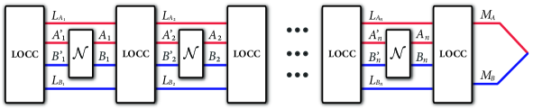
Figure 3: A protocol for LOCC-assisted entanglement distillation that uses a bipartite quantum channel $\mathcal{N}$ $n$ times. Every channel use is interleaved by an LOCC bipartite channel. The goal of such a protocol is to produce an approximate maximally entangled state in the systems $M_{A}$ and $M_{B}$, where Alice possesses system $M_{A}$ and Bob system $M_{B}$.

The most general protocol for distilling entanglement from a bipartite channel, as depicted in Figure 3, has the following form. Alice and Bob are spatially separated, and they are allowed to undergo a bipartite quantum channel $\mathcal{N}_{A^{\prime}B^{\prime}\rightarrow AB}$. Alice holds systems labeled by $A^{\prime},A$ whereas Bob holds $B^{\prime},B$. They begin by performing an LOCC channel $\mathcal{L}_{\varnothing\rightarrow L_{A_{1}}A_{1}^{\prime}B_{1}^{\prime}L_{B_{1}}}^{(1)}$, which leads to a separable state $\rho_{L_{A_{1}}A_{1}^{\prime}B_{1}^{\prime}L_{B_{1}}}^{(1)}$, where $L_{A_{1}},L_{B_{1}}$ are finite-dimensional systems of arbitrary size and $A_{1}^{\prime},B_{1}^{\prime}$ are input systems to the first channel use. Alice and Bob send systems $A_{1}^{\prime}$ and $B_{1}^{\prime}$, respectively, through the first channel use, which yields the output state $\sigma_{L_{A_{1}}A_{1}B_{1}L_{B_{1}}}^{(1)}:=\mathcal{N}_{A_{1}^{\prime}B_{1}^{\prime}\rightarrow A_{1}B_{1}}(\rho_{L_{A_{1}}A_{1}^{\prime}B_{1}^{\prime}L_{B_{1}}}^{(1)})$. Alice and Bob then perform the LOCC channel $\mathcal{L}_{L_{A_{1}}A_{1}B_{1}L_{B_{1}}\rightarrow L_{A_{2}}A_{2}^{\prime}B_{2}^{\prime}L_{B_{2}}}^{(2)}$, which leads to the state $\rho_{L_{A_{2}}A_{2}^{\prime}B_{2}^{\prime}L_{B_{2}}}^{(2)}:=\mathcal{L}_{L_{A_{1}}A_{1}B_{1}L_{B_{1}}\rightarrow L_{A_{2}}A_{2}^{\prime}B_{2}^{\prime}L_{B_{2}}}^{(2)}(\sigma_{L_{A_{1}}A_{1}B_{1}L_{B_{1}}}^{(1)})$. Both parties then send systems $A_{2}^{\prime},B_{2}^{\prime}$ through the second channel use $\mathcal{N}_{A_{2}^{\prime}B_{2}^{\prime}\rightarrow A_{2}B_{2}}$, which yields the state

$$\sigma_{L_{A_{2}}A_{2}B_{2}L_{B_{2}}}^{(2)}:=\mathcal{N}_{A_{2}^{\prime}B_{2}^{\prime}\rightarrow A_{2}B_{2}}(\rho_{L_{A_{2}}A_{2}^{\prime}B_{2}^{\prime}L_{B_{2}}}^{(2)}).$$ (3.23)

They iterate this process such that the protocol makes use of the channel $n$ times. In general, we have the following states for the $i$th use, for $i\in\{2,3,\ldots,n\}$:

$$\rho_{L_{A_{i}}A_{i}^{\prime}B_{i}^{\prime}L_{B_{i}}}^{(i)} :=\mathcal{L}_{L_{A_{i-1}}A_{i-1}B_{i-1}L_{B_{i-1}}\rightarrow L_{A_{i}}A_{i}^{\prime}B_{i}^{\prime}L_{B_{i}}}^{(i)}(\sigma_{L_{A_{i-1}}A_{i-1}B_{i-1}L_{B_{i-1}}}^{(i-1)}),$$ (3.24)

$$\sigma_{L_{A_{i}}A_{i}B_{i}L_{B_{i}}}^{(i)} :=\mathcal{N}_{A_{i}^{\prime}B_{i}^{\prime}\rightarrow A_{i}B_{i}}(\rho_{L_{A_{i}}A_{i}^{\prime}B_{i}^{\prime}L_{B_{i}}}^{(i)}),$$ (3.25)

where $\mathcal{L}_{L_{A_{i-1}}A_{i-1}B_{i-1}L_{B_{i-1}}\rightarrow L_{A_{i}}A_{i}^{\prime}B_{i}^{\prime}L_{B_{i}}}^{(i)}$ is an LOCC channel. In the final step of the protocol, an LOCC channel $\mathcal{L}_{L_{A_{n}}A_{n}B_{n}L_{B_{n}}\rightarrow M_{A}M_{B}}^{(n+1)}$ is applied, that generates the final state:

$$\omega_{M_{A}M_{B}}:=\mathcal{P}_{L_{A_{n}}A_{n}B_{n}L_{B_{n}}\rightarrow M_{A}M_{B}}^{(n+1)}(\sigma_{L_{A_{n}}A_{n}^{\prime}B_{n}^{\prime}L_{B_{n}}}^{(n)}),$$ (3.26)

where $M_{A}$ and $M_{B}$ are held by Alice and Bob, respectively.

The goal of the protocol is for Alice and Bob to distill entanglement in the end; i.e., the final state $\omega_{M_{A}M_{B}}$ should be close to a maximally entangled state. For a fixed $n,\ M\in\mathbb{N},\ \varepsilon\in[0,1]$, the original protocol is an $(n,M,\varepsilon)$ protocol if the channel is used $n$ times as discussed above, $|M_{A}|=|M_{B}|=M$, and if $F(\omega_{M_{A}M_{B}},\Phi_{M_{A}M_{B}})=\left\langle\Phi\right|_{M_{A}M_{B}}\omega_{M_{A}M_{B}}\left|\Phi\right\rangle_{AB}\geq 1-\varepsilon,$ where $\Phi_{M_{A}M_{B}}$ is the maximally entangled state. A rate $R$ is said to be achievable for entanglement distillation if for all $\varepsilon\in(0,1]$, $\delta>0$, and sufficiently large $n$, there exists an $(n,2^{n(R-\delta)},\varepsilon)$ protocol. The distillable entanglement of $\mathcal{N}$, denoted as $Q(\mathcal{N})$, is equal to the supremum of all achievable rates.

The recent work [DBW17] defined the max-Rains information $R_{\max}(\mathcal{N})$ of a bipartite quantum channel $\mathcal{N}_{A^{\prime}B^{\prime}\rightarrow AB}$ as follows:

$$R_{\max}(\mathcal{N}):=\log\Gamma(\mathcal{N}),$$ (3.27)

where $\Gamma(\mathcal{N})$ is the solution to the following semi-definite program:

$$\inf\{\left\|\operatorname{Tr}_{AB}\{V_{S_{A}ABS_{B}}+Y_{S_{A}ABS_{B}}\}\right\|_{\infty}:V,Y\geq 0,\ T_{BS_{B}}(V_{S_{A}ABS_{B}}-Y_{S_{A}ABS_{B}})\geq J_{S_{A}ABS_{B}}^{\mathcal{N}}\},$$ (3.28)

such that $S_{A}\simeq A^{\prime}$, and $S_{B}\simeq B^{\prime}$. One of the main results of [DBW17] is the following bound $Q(\mathcal{N})\leq R_{\max}(\mathcal{N})$, establishing the max-Rains information as a fundamental limitation on the distillable entanglement of any bipartite channel.

One of the key properties of the max-Rains information is that it does not increase under amortization; i.e., the following inequality is satisfied. Let $\rho_{L_{A}A^{\prime}B^{\prime}L_{B}}$ be a state, and let $\mathcal{N}_{A^{\prime}B^{\prime}\rightarrow AB}$ be a bipartite channel. Then

$$R_{\max}(L_{A}A;BL_{B})_{\omega}\leq R_{\max}(L_{A}A^{\prime};B^{\prime}L_{B})_{\rho}+R_{\max}(\mathcal{N}),$$ (3.29)

where $\omega_{L_{A}ABL_{B}}=\mathcal{N}_{A^{\prime}B^{\prime}\rightarrow AB}(\rho_{L_{A}A^{\prime}B^{\prime}L_{B}})$ and the max-Rains relative entropy of a state $\sigma_{CD}$ is

$$R_{\max}(C;D)_{\sigma}:=\inf\{\lambda:\sigma_{CD}\leq 2^{\lambda}\omega_{CD},\ \omega_{CD}\geq 0,\ \left\|T_{D}(\omega_{CD})\right\|_{1}\leq 1\}.$$ (3.30)

The amortization inequality above is stronger than additivity, and it is one of the main technical tools needed for establishing the key inequality $Q(\mathcal{N})\leq R_{\max}(\mathcal{N})$.

3.4 Exact distillable entanglement of bipartite channels

Another interesting question, dual to the exact entanglement cost question proposed above, is the exact distillable entanglement of a bipartite channel. The setting for this problem is the same as that outlined in the previous section, but we demand that the error $\varepsilon$ is exactly equal to zero. We again consider the free operations to be completely PPT-preserving operations, so that a solution to this problem will give bounds for the exact distillable entanglement with LOCC.

To start out, we should recall developments for bipartite states. The most significant progress on the exact distillable entanglement of a bipartite state $\rho_{AB}$ has been made recently in [WD17b]. To begin with, let us define the one-shot exact distillable entanglement of a bipartite state $\rho_{AB}$ as

$$E_{\text{PPT}}^{(1,d)}(\rho_{AB}):=\sup\{\log_{2}d:\mathcal{P}_{AB\rightarrow\hat{A}\hat{B}}(\rho_{AB})=\Phi_{\hat{A}\hat{B}}^{d}\},$$ (3.31)

where $\mathcal{P}_{AB\rightarrow\hat{A}\hat{B}}$ is a completely PPT-preserving operation. In [WD17b], it was shown that $E_{\text{PPT}}^{(1,d)}(\rho_{AB})$ is given by the following optimization:

$$E_{\text{PPT}}^{(1,d)}(\rho_{AB})=-\log W_{0}(\rho_{AB}),\qquad W_{0}(\rho_{AB}):=\inf\{\left\|T_{B}(R_{AB})\right\|_{\infty}:P_{AB}\leq R_{AB}\leq I_{AB}\},$$ (3.32)

with $P_{AB}$ the projection onto the support of the state $\rho_{AB}$. The exact entanglement cost of a bipartite state $\rho_{AB}$ is then defined as the regularization of the above:

$$E_{\text{PPT}}^{d}(\rho_{AB}):=\lim_{n\rightarrow\infty}\frac{1}{n}E_{\text{PPT}}^{(1,d)}(\rho_{AB}^{\otimes n}).$$ (3.33)

By relaxing one of the constraints for $W_{0}$ above, we get the following quantity [WD17b], called the min-Rains relative entropy:

$$M(\rho_{AB}):=\inf\{\left\|T_{B}(R_{AB})\right\|_{\infty}:P_{AB}\leq R_{AB}\},$$ (3.34)

and then it follows that

$$E_{\text{PPT}}^{(1,d)}(\rho_{AB})\leq E_{M}(\rho_{AB}):=-\log_{2}M(\rho_{AB}).$$ (3.35)

However, a significant property of $E_{M}(\rho_{AB})$ is that it is additive [WD17b]:

$$E_{M}(\rho_{AB}\otimes\sigma_{A^{\prime}B^{\prime}})=E_{M}(\rho_{AB})+E_{M}(\sigma_{A^{\prime}B^{\prime}}).$$ (3.36)

By exploiting this property, the following single-letter, efficiently computable upper bound on the exact distillable entanglement follows [WD17b]:

$$E_{\text{PPT}}^{d}(\rho_{AB})\leq E_{M}(\rho_{AB}).$$ (3.37)

Some key questions for this task are as follows: Is the inequality in (3.37) tight? This would involve showing that one of the constraints in (3.32) becomes negligible in the asymptotic limit of many copies of $\rho_{AB}$. If it is true, it would be a strong counterpart to the finding in (3.19). We can also analyze the exact distillable entanglement of a point-to-point quantum channel $\mathcal{N}_{A\rightarrow B}$, and in light of the result in (3.35), it is natural to wonder whether

$$E_{\text{PPT}}^{(1,d)}(\mathcal{N}_{A\rightarrow B})\leq E_{M}(\mathcal{N}_{A\rightarrow B}),$$ (3.38)

where the one-shot distillable entanglement of a channel is given by

$$E_{\text{PPT}}^{(1,d)}(\mathcal{N}_{A\rightarrow B}):=\sup\{\log_{2}d:\mathcal{P}_{A^{\prime}BB^{\prime}\rightarrow\hat{A}\hat{B}}(\mathcal{N}_{A\rightarrow B}(\rho_{A^{\prime}AB^{\prime}}))=\Phi_{\hat{A}\hat{B}}^{d}\},$$ (3.39)

with $\rho_{A^{\prime}AB^{\prime}}$ a PPT state and $\mathcal{P}_{A^{\prime}BB^{\prime}\rightarrow\hat{A}\hat{B}}$ a completely PPT-preserving channel, and the min-Rains information of a channel $\mathcal{N}_{A\rightarrow B}$ is defined as the optimized min-Rains relative entropy:

$$E_{M}(\mathcal{N}_{A\rightarrow B}):=\sup_{\psi_{RA}}E_{M}(\mathcal{N}_{A\rightarrow B}(\psi_{RA})),$$ (3.40)

where the optimization is with respect to pure states $\psi_{RA}$ with system $R$ isomorphic to system $A$. From here, a natural next question is to determine bounds on the exact distillable entanglement of a bipartite channel.

4 Entanglement measures for bipartite channels

Here we develop entanglement measures for bipartite channels, including logarithmic negativity, $\kappa$ entanglement, and generalized Rains information. We begin with some background and then develop the aforementioned measures.

4.1 Entropies and information

The quantum entropy of a density operator $\rho_{A}$ is defined as [vN32]

$$S(A)_{\rho}:=S(\rho_{A})=-\operatorname{Tr}[\rho_{A}\log_{2}\rho_{A}].$$ (4.1)

The conditional quantum entropy $S(A|B)_{\rho}$ of a density operator $\rho_{AB}$ of a composite system $AB$ is defined as

$$S(A|B)_{\rho}\coloneqq S(AB)_{\rho}-S(B)_{\rho}.$$ (4.2)

The coherent information $I(A\rangle B)_{\rho}$ of a density operator $\rho_{AB}$ of a composite system $AB$ is defined as [SN96]

$$I(A\rangle B)_{\rho}\coloneqq-S(A|B)_{\rho}=S(B)_{\rho}-S(AB)_{\rho}.$$ (4.3)

The quantum relative entropy of two quantum states is a measure of their distinguishability. For $\rho\in\mathcal{D}(\mathcal{H})$ and $\sigma\in\mathcal{B}_{+}(\mathcal{H})$, it is defined as [Ume62]

$$D(\rho\|\sigma):=\left\{\begin{tabular}[]{c c}$\operatorname{Tr}\{\rho[\log_{2}\rho-\log_{2}\sigma]\}$,&$\operatorname{supp}(\rho)\subseteq\operatorname{supp}(\sigma)$\\ $+\infty$,&otherwise.\end{tabular}\right.$$ (4.4)

The quantum relative entropy is non-increasing under the action of positive trace-preserving maps [MHR17], which is the statement that $D(\rho\|\sigma)\geq D(\mathcal{M}(\rho)\|\mathcal{M}{(\sigma)})$ for any two density operators $\rho$ and $\sigma$ and a positive trace-preserving map $\mathcal{M}$ (this inequality applies to quantum channels as well [Lin75], since every completely positive map is also a positive map by definition).

4.2 Generalized divergence and generalized relative entropies

A quantity is called a generalized divergence [PV10, SW12] if it satisfies the following monotonicity (data-processing) inequality for all density operators $\rho$ and $\sigma$ and quantum channels $\mathcal{N}$:

$$\mathbf{D}(\rho\|\sigma)\geq\mathbf{D}(\mathcal{N}(\rho)\|\mathcal{N}(\sigma)).$$ (4.5)

As a direct consequence of the above inequality, any generalized divergence satisfies the following two properties for an isometry $U$ and a state $\tau$ [WWY14]:

$$\mathbf{D}(\rho\|\sigma) =\mathbf{D}(U\rho U^{\dagger}\|U\sigma U^{\dagger}),$$ (4.6)

$$\mathbf{D}(\rho\|\sigma) =\mathbf{D}(\rho\otimes\tau\|\sigma\otimes\tau).$$ (4.7)

The sandwiched Rényi relative entropy [MLDS⁺13, WWY14] is denoted as $\widetilde{D}_{\alpha}(\rho\|\sigma)$ and defined for $\rho\in\mathcal{D}(\mathcal{H})$, $\sigma\in\mathcal{B}_{+}(\mathcal{H})$, and $\forall\alpha\in(0,1)\cup(1,\infty)$ as

$$\widetilde{D}_{\alpha}(\rho\|\sigma):=\frac{1}{\alpha-1}\log_{2}\operatorname{Tr}\left\{\left(\sigma^{\frac{1-\alpha}{2\alpha}}\rho\sigma^{\frac{1-\alpha}{2\alpha}}\right)^{\alpha}\right\},$$ (4.8)

but it is set to $+\infty$ for $\alpha\in(1,\infty)$ if $\operatorname{supp}(\rho)\nsubseteq\operatorname{supp}(\sigma)$. The sandwiched Rényi relative entropy obeys the following “monotonicity in $\alpha$” inequality [MLDS⁺13]: for $\alpha,\beta\in(0,1)\cup(1,\infty)$,

$$\widetilde{D}_{\alpha}(\rho\|\sigma)\leq\widetilde{D}_{\beta}(\rho\|\sigma)\quad\text{ if }\quad\alpha\leq\beta.$$ (4.9)

The following lemma states that the sandwiched Rényi relative entropy $\widetilde{D}_{\alpha}(\rho\|\sigma)$ is a particular generalized divergence for certain values of $\alpha$.

Lemma 1 ([FL13])

Let $\mathcal{N}:\mathcal{B}_{+}(\mathcal{H}_{A})\to\mathcal{B}_{+}(\mathcal{H}_{B})$ be a quantum channel and let $\rho_{A}\in\mathcal{D}(\mathcal{H}_{A})$ and $\sigma_{A}\in\mathcal{B}_{+}(\mathcal{H}_{A})$. Then, for all $\alpha\in\left[1/2,1\right)\cup(1,\infty)$

$$\widetilde{D}_{\alpha}(\rho\|\sigma)\geq\widetilde{D}_{\alpha}(\mathcal{N}(\rho)\|\mathcal{N}(\sigma)).$$ (4.10)

See [Wil18b] for an alternative proof of Lemma 1.

In the limit $\alpha\to 1$, the sandwiched Rényi relative entropy $\widetilde{D}_{\alpha}(\rho\|\sigma)$ converges to the quantum relative entropy [MLDS⁺13, WWY14]:

$$\lim_{\alpha\to 1}\widetilde{D}_{\alpha}(\rho\|\sigma):=D_{1}(\rho\|\sigma)=D(\rho\|\sigma).$$ (4.11)

In the limit $\alpha\to\infty$, the sandwiched Rényi relative entropy $\widetilde{D}_{\alpha}(\rho\|\sigma)$ converges to the max-relative entropy [MLDS⁺13], which is defined as [Dat09b, Dat09a]

$$D_{\max}(\rho\|\sigma)=\inf\{\lambda:\ \rho\leq 2^{\lambda}\sigma\},$$ (4.12)

and if $\operatorname{supp}(\rho)\nsubseteq\operatorname{supp}(\sigma)$ then $D_{\max}(\rho\|\sigma)=\infty$.

4.3 Entanglement measures for bipartite states

Let $\operatorname{Ent}(A;B)_{\rho}$ denote an entanglement measure [HHHH09] that is evaluated for a bipartite state $\rho_{AB}$. The basic property of an entanglement measure is that it should be an LOCC monotone [HHHH09], i.e., non-increasing under the action of an LOCC channel. Given such an entanglement measure, one can define the entanglement $\operatorname{Ent}(\mathcal{M})$ of a channel $\mathcal{M}_{A\to B}$ in terms of it by optimizing over all pure, bipartite states that can be input to the channel:

$$\operatorname{Ent}(\mathcal{M})=\sup_{\psi_{LA}}\operatorname{Ent}(L;B)_{\omega},$$ (4.13)

where $\omega_{LB}=\mathcal{M}_{A\to B}(\psi_{LA})$. Due to the properties of an entanglement measure and the well known Schmidt decomposition theorem, it suffices to optimize over pure states $\psi_{LA}$ such that $L\simeq A$ (i.e., one does not achieve a higher value of $\operatorname{Ent}(\mathcal{M})$ by optimizing over mixed states with unbounded reference system $L$). In an information-theoretic setting, the entanglement $\operatorname{Ent}(\mathcal{M})$ of a channel $\mathcal{M}$ characterizes the amount of entanglement that a sender $A$ and receiver $B$ can generate by using the channel if they do not share entanglement prior to its use.

Alternatively, one can consider the amortized entanglement $\operatorname{Ent}_{A}(\mathcal{M})$ of a channel $\mathcal{M}_{A\to B}$ as the following optimization [KW17] (see also [LHL03, BHLS03, CMH17, BDGDMW17, RKB⁺18]):

$$\operatorname{Ent}_{A}(\mathcal{M})\coloneqq\sup_{\rho_{L_{A}AL_{B}}}\left[\operatorname{Ent}(L_{A};BL_{B})_{\tau}-\operatorname{Ent}(L_{A}A;L_{B})_{\rho}\right],$$ (4.14)

where $\tau_{L_{A}BL_{B}}=\mathcal{M}_{A\to B}(\rho_{L_{A}AL_{B}})$ and $\rho_{L_{A}AL_{B}}$ is a state. The supremum is with respect to all states $\rho_{L_{A}AL_{B}}$ and the systems $L_{A},L_{B}$ are finite-dimensional but could be arbitrarily large. Thus, in general, $\operatorname{Ent}_{A}(\mathcal{M})$ need not be computable. The amortized entanglement quantifies the net amount of entanglement that can be generated by using the channel $\mathcal{M}_{A\to B}$, if the sender and the receiver are allowed to begin with some initial entanglement in the form of the state $\rho_{L_{A}AL_{B}}$. That is, $\operatorname{Ent}(L_{A}A;L_{B})_{\rho}$ quantifies the entanglement of the initial state $\rho_{L_{A}AL_{B}}$, and $\operatorname{Ent}(L_{A};BL_{B})_{\tau}$ quantifies the entanglement of the final state produced after the action of the channel.

The Rains relative entropy of a state $\rho_{AB}$ is defined as [Rai01, ADMVW02]

$$R(A;B)_{\rho}\coloneqq\min_{\sigma_{AB}\in\operatorname{PPT}^{\prime}(A:B)}D(\rho_{AB}\|\sigma_{AB}),$$ (4.15)

and it is monotone non-increasing under the action of a completely PPT-preserving quantum channel $\mathcal{P}_{A^{\prime}B^{\prime}\to AB}$, i.e.,

$$R(A^{\prime};B^{\prime})_{\rho}\geq R(A;B)_{\omega},$$ (4.16)

where $\omega_{AB}=\mathcal{P}_{A^{\prime}B^{\prime}\to AB}(\rho_{A^{\prime}B^{\prime}})$. The sandwiched Rains relative entropy of a state $\rho_{AB}$ is defined as follows [TWW17]:

$$\widetilde{R}_{\alpha}(A;B)_{\rho}\coloneqq\min_{\sigma_{AB}\in\operatorname{PPT}^{\prime}(A:B)}\widetilde{D}_{\alpha}(\rho_{AB}\|\sigma_{AB}).$$ (4.17)

The max-Rains relative entropy of a state $\rho_{AB}$ is defined as [WD16b]

$$R_{\max}(A;B)_{\rho}\coloneqq\min_{\sigma_{AB}\in\operatorname{PPT}^{\prime}(A:B)}D_{\max}(\rho_{AB}\|\sigma_{AB}).$$ (4.18)

The max-Rains information of a quantum channel $\mathcal{M}_{A\to B}$ is defined as [WFD17]

$$R_{\max}(\mathcal{M})\coloneqq\max_{\phi_{SA}}R_{\max}(S;B)_{\omega},$$ (4.19)

where $\omega_{SB}=\mathcal{M}_{A\to B}(\phi_{SA})$ and $\phi_{SA}$ is a pure state, with $\dim(\mathcal{H}_{S})=\dim(\mathcal{H}_{A})$. The amortized max-Rains information of a channel $\mathcal{M}_{A\to B}$, denoted as $R_{\max,A}(\mathcal{M})$, is defined by replacing $\operatorname{Ent}$ in (4.14) with the max-Rains relative entropy $R_{\max}$ [BW18]. It was shown in [BW18] that amortization does not enhance the max-Rains information of an arbitrary point-to-point channel, i.e.,

$$R_{\max,A}(\mathcal{M})=R_{\max}(\mathcal{M}).$$ (4.20)

Recently, in [WD16a, Eq. (8)] (see also [WFD17]), the max-Rains relative entropy of a state $\rho_{AB}$ was expressed as

$$R_{\max}(A;B)_{\rho}=\log_{2}W(A;B)_{\rho},$$ (4.21)

where $W(A;B)_{\rho}$ is the solution to the following semi-definite program:

minimize $$\ \operatorname{Tr}\{C_{AB}+D_{AB}\}$$

subject to $$\ C_{AB},D_{AB}\geq 0,$$

$$\ \operatorname{T}_{B}(C_{AB}-D_{AB})\geq\rho_{AB}.$$ (4.22)

Similarly, in [WFD17, Eq. (21)], the max-Rains information of a quantum channel $\mathcal{M}_{A\to B}$ was expressed as

$$R_{\max}(\mathcal{M})=\log\Gamma(\mathcal{M}),$$ (4.23)

where $\Gamma(\mathcal{M})$ is the solution to the following semi-definite program:

minimize $$\ \left\|{\operatorname{Tr}_{B}\{V_{SB}+Y_{SB}\}}\right\|_{\infty}$$

subject to $$\ Y_{SB},V_{SB}\geq 0,$$

$$\ \operatorname{T}_{B}(V_{SB}-Y_{SB})\geq J^{\mathcal{M}}_{SB}.$$ (4.24)

The sandwiched relative entropy of entanglement of a bipartite state $\rho_{AB}$ is defined as [WTB17]

$$\widetilde{E}_{\alpha}(A;B)_{\rho}\coloneqq\min_{\sigma_{AB}\in\operatorname{SEP}(A:B)}\widetilde{D}_{\alpha}(\rho_{AB}\|\sigma_{AB}).$$ (4.25)

In the limit $\alpha\to 1$, $\widetilde{E}_{\alpha}(A;B)_{\rho}$ converges to the relative entropy of entanglement [VP98], i.e.,

$$\lim_{\alpha\to 1}\widetilde{E}_{\alpha}(A;B)_{\rho} =E(A;B)_{\rho}$$ (4.26)

$$\coloneqq\min_{\sigma_{AB}\in\operatorname{SEP}(A:B)}D(\rho_{AB}\|\sigma_{AB}).$$ (4.27)

The max-relative entropy of entanglement [Dat09b, Dat09a] is defined for a bipartite state $\rho_{AB}$ as

$$E_{\max}(A;B)_{\rho}\coloneqq\min_{\sigma_{AB}\in\operatorname{SEP}(A:B)}D_{\max}(\rho_{AB}\|\sigma_{AB}).$$ (4.28)

The max-relative entropy of entanglement $E_{\max}(\mathcal{M})$ of a channel $\mathcal{M}_{A\to B}$ is defined as in (4.13), by replacing $\operatorname{Ent}$ with $E_{\max}$ [CMH17]. It was shown in [CMH17] that amortization does not increase max-relative entropy of entanglement of a channel $\mathcal{M}_{A\to B}$, i.e.,

$$E_{\max,A}(\mathcal{M})=E_{\max}(\mathcal{M}).$$ (4.29)

4.4 Negativity of a bipartite state

Given a bipartite state, its logarithmic negativity is defined as [VW02, Ple05]

$$E_{N}(\rho_{AB}):=\log\left\|T_{B}(\rho_{AB})\right\|_{1}.$$ (4.30)

The idea of this quantity is to quantify the deviation of a bipartite state from being PPT. If it is indeed PPT, then $E_{N}(\rho_{AB})=0$. If not, then $E_{N}(\rho_{AB})>0$.

By utilizing Holder duality, it is possible to write the above as a semi-definite program:

$$E_{N}(\rho_{AB})=\log\sup_{R_{AB}}\left\{\operatorname{Tr}[R_{AB}\rho_{AB}]:-I_{AB}\leq T_{B}(R_{AB})\leq I_{AB}\right\},$$ (4.31)

where the optimization is with respect to Hermitian $R_{AB}$. By utilizing semi-definite programming duality, we can also write $E_{N}(\rho_{AB})$ in terms of its dual semi-definite program as

$$E_{N}(\rho_{AB})=\log\inf_{K_{AB},L_{AB}\geq 0}\left\{\operatorname{Tr}[K_{AB}+L_{AB}]:T_{B}(K_{AB}-L_{AB})=\rho_{AB}\right\}.$$ (4.32)

The max-Rains relative entropy of a bipartite state is defined as follows [WD16a]:

$$R_{\max}(\rho_{AB}):=\inf_{\sigma_{AB}\geq 0,E_{N}(\sigma_{AB})\leq 0}D_{\max}(\rho_{AB}\|\sigma_{AB}).$$ (4.33)

It can be written as the following semi-definite program:

$$R_{\max}(\rho_{AB})=\log\sup_{R_{AB}\geq 0}\left\{\operatorname{Tr}[R_{AB}\rho_{AB}]:-I_{AB}\leq T_{B}(R_{AB})\leq I_{AB}\right\},$$ (4.34)

with the dual

$$R_{\max}(\rho_{AB})=\log\inf_{K_{AB},L_{AB}\geq 0}\left\{\operatorname{Tr}[K_{AB}+L_{AB}]:T_{B}(K_{AB}-L_{AB})\geq\rho_{AB}\right\}.$$ (4.35)

It is clear that

$$R_{\max}(\rho_{AB})\leq E_{N}(\rho_{AB}),$$ (4.36)

since the primal for $R_{\max}(\rho_{AB})$ is obtained from the primal for $E_{N}(\rho_{AB})$ by restricting the optimization to $R_{AB}\geq 0$. Alternatively, the dual of $R_{\max}(\rho_{AB})$ is obtained from the dual of $E_{N}(\rho_{AB})$ by relaxing the equality constraint $\rho_{AB}=T_{B}(K_{AB}-L_{AB})$.

Finally, note that we can define Rains relative entropy of a bipartite state much more generally in terms of a generalized divergence $\mathbf{D}$ as

$$\mathbf{R}(\rho_{AB}):=\inf_{\sigma_{AB}\geq 0,E_{N}(\sigma_{AB})\leq 0}\mathbf{D}(\rho_{AB}\|\sigma_{AB})$$ (4.37)

4.5 Negativity of a bipartite channel

Let us define the logarithmic negativity of a bipartite channel $\mathcal{N}_{A^{\prime}B^{\prime}\rightarrow AB}$ as

$$E_{N}(\mathcal{N}):=\log\left\|T_{B}\circ\mathcal{N}_{A^{\prime}B^{\prime}\rightarrow AB}\circ T_{B^{\prime}}\right\|_{\Diamond},$$ (4.38)

where the diamond norm [Kit97] of a bipartite linear, Hermitian-preserving map $\mathcal{P}_{A^{\prime}B^{\prime}\rightarrow AB}$ is given by

$$\left\|\mathcal{P}_{A^{\prime}B^{\prime}\rightarrow AB}\right\|_{\Diamond}:=\log\sup_{\psi_{S_{A}A^{\prime}B^{\prime}S_{B}}}\left\|\mathcal{P}_{A^{\prime}B^{\prime}\rightarrow AB}(\psi_{S_{A}A^{\prime}B^{\prime}S_{B}})\right\|_{1}.$$ (4.39)

Thus, more generally, $E_{N}(\mathcal{N})$ can be defined in the above way if $\mathcal{N}_{A^{\prime}B^{\prime}\rightarrow AB}$ is an arbitrary linear, Hermitian-preserving map. Note that $E_{N}(\mathcal{N})$ reduces to the well known logarithmic negativity of a point-to-point channel [HW01] when the bipartite channel is indeed a point-to-point channel.

A bipartite channel $\mathcal{N}_{A^{\prime}B^{\prime}\rightarrow AB}$ is called completely PPT preserving (C-PPT-P) if the map $T_{B}\circ\mathcal{N}_{A^{\prime}B^{\prime}\rightarrow AB}\circ T_{B^{\prime}}$ is completely positive [Rai99, Rai01]. Thus, the measure in (4.38) quantifies the deviation of a bipartite channel from being C-PPT-P. Indeed, if $\mathcal{N}_{A^{\prime}B^{\prime}\rightarrow AB}$ is C-PPT-P, then $E_{N}(\mathcal{N})=0$. Otherwise, $E_{N}(\mathcal{N})>0$.

Proposition 1

The logarithmic negativity of a bipartite channel $\mathcal{N}_{A^{\prime}B^{\prime}\rightarrow AB}$ can be written as the following primal SDP:

$$\sup_{\rho,R}\left\{\begin{array}[c]{c}\operatorname{Tr}[T_{BS_{B}}(J_{S_{A}ABS_{B}}^{\mathcal{N}})R_{S_{A}ABS_{B}}]:\rho_{S_{A}S_{B}}\geq 0,\operatorname{Tr}[\rho_{S_{A}S_{B}}]\leq 1,\\ -\rho_{S_{A}S_{B}}\otimes I_{AB}\leq R_{S_{A}ABS_{B}}\leq\rho_{S_{A}S_{B}}\otimes I_{AB}\end{array}\right\},$$ (4.40)

where $J_{S_{A}ABS_{B}}^{\mathcal{N}}$ is the Choi operator of the channel $\mathcal{N}_{A^{\prime}B^{\prime}\rightarrow AB}$ and the optimization is with respect to Hermitian $R_{S_{A}ABS_{B}}$. The dual SDP is given by

$$\inf\left\{\begin{array}[c]{c}\left\|\operatorname{Tr}_{AB}[V_{S_{A}ABS_{B}}+Y_{S_{A}ABS_{B}}]\right\|_{\infty}:V_{S_{A}ABS_{B}},Y_{S_{A}ABS_{B}}\geq 0,\\ T_{BS_{B}}(V_{S_{A}ABS_{B}}-Y_{S_{A}ABS_{B}})=J_{S_{A}ABS_{B}}^{\mathcal{N}}\end{array}\right\}.$$ (4.41)

Proof. Starting from the definition, we find that

$$\sup_{\psi}\left\|(T_{B}\circ\mathcal{N}_{A^{\prime}B^{\prime}\rightarrow AB}\circ T_{B^{\prime}})(\psi_{S_{A}A^{\prime}B^{\prime}S_{B}})\right\|_{1}$$ (4.42)

$$=\sup_{\psi,R}\left\{\operatorname{Tr}[(T_{B}\circ\mathcal{N}_{A^{\prime}B^{\prime}\rightarrow AB}\circ T_{B^{\prime}})(\psi_{S_{A}A^{\prime}B^{\prime}S_{B}})R_{S_{A}ABS_{B}}]:\left\|R_{S_{A}ABS_{B}}\right\|_{\infty}\leq 1\right\}$$ (4.43)

$$=\sup_{\rho,R}\left\{\begin{array}[c]{c}\operatorname{Tr}[(T_{B}\circ\mathcal{N}_{A^{\prime}B^{\prime}\rightarrow AB}\circ T_{B^{\prime}})(\rho_{S_{A}S_{B}}^{1/2}\Gamma_{S_{A}A^{\prime}B^{\prime}S_{B}}\rho_{S_{A}S_{B}}^{1/2})R_{S_{A}ABS_{B}}]:\\ \rho_{S_{A}S_{B}}\geq 0,\operatorname{Tr}[\rho_{S_{A}S_{B}}]=1,\left\|R_{S_{A}ABS_{B}}\right\|_{\infty}\leq 1\end{array}\right\}$$ (4.46)

$$=\sup_{\rho,R}\left\{\begin{array}[c]{c}\operatorname{Tr}[\rho_{S_{A}S_{B}}^{1/2}T_{BS_{B}}(J_{S_{A}ABS_{B}}^{\mathcal{N}})\rho_{S_{A}S_{B}}^{1/2}R_{S_{A}ABS_{B}}]:\rho_{S_{A}S_{B}}\geq 0,\operatorname{Tr}[\rho_{S_{A}S_{B}}]=1,\\ -I_{S_{A}ABS_{B}}\leq R_{S_{A}ABS_{B}}\leq I_{S_{A}ABS_{B}}\end{array}\right\}$$ (4.49)

$$=\sup_{\rho,R}\left\{\begin{array}[c]{c}\operatorname{Tr}[T_{BS_{B}}(J_{S_{A}ABS_{B}}^{\mathcal{N}})\rho_{S_{A}S_{B}}^{1/2}R_{S_{A}ABS_{B}}\rho_{S_{A}S_{B}}^{1/2}]:\rho_{S_{A}S_{B}}\geq 0,\operatorname{Tr}[\rho_{S_{A}S_{B}}]=1,\\ -I_{S_{A}ABS_{B}}\leq R_{S_{A}ABS_{B}}\leq I_{S_{A}ABS_{B}}\end{array}\right\}$$ (4.52)

$$=\sup_{\rho,R}\left\{\begin{array}[c]{c}\operatorname{Tr}[T_{BS_{B}}(J_{S_{A}ABS_{B}}^{\mathcal{N}})R_{S_{A}ABS_{B}}]:\rho_{S_{A}S_{B}}\geq 0,\operatorname{Tr}[\rho_{S_{A}S_{B}}]=1,\\ -\rho_{S_{A}S_{B}}\otimes I_{AB}\leq R_{S_{A}ABS_{B}}\leq\rho_{S_{A}S_{B}}\otimes I_{AB}\end{array}\right\}$$ (4.55)

Thus, it is clearly an SDP. By employing standard techniques, we find that the dual is given as stated in the proposition.   

Proposition 2 (Faithfulness)

The logarithmic negativity of a bipartite channel $\mathcal{N}_{A^{\prime}B^{\prime}\rightarrow AB}$ obeys the following faithfulness condition:

$$E_{N}(\mathcal{N})\geq 0\text{ and }E_{N}(\mathcal{N})=0\text{ if and only if }\mathcal{N}\in\text{{C-PPT-P}.}$$ (4.56)

Proof. The first inequality is equivalent to the following one:

$$\left\|T_{B}\circ\mathcal{N}_{A^{\prime}B^{\prime}\rightarrow AB}\circ T_{B^{\prime}}\right\|_{\Diamond}\geq 1.$$ (4.57)

Pick $\psi_{S_{A}A^{\prime}B^{\prime}S_{B}}$ in (4.39) to be $\Phi_{S_{A}A^{\prime}}\otimes\Phi_{B^{\prime}S_{B}}$. Then

$$(T_{B}\circ\mathcal{N}_{A^{\prime}B^{\prime}\rightarrow AB}\circ T_{B^{\prime}})(\Phi_{S_{A}A^{\prime}}\otimes\Phi_{B^{\prime}S_{B}}) =(T_{B}\circ\mathcal{N}_{A^{\prime}B^{\prime}\rightarrow AB}\circ T_{S_{B}})(\Phi_{S_{A}A^{\prime}}\otimes\Phi_{B^{\prime}S_{B}})$$ (4.58)

$$=(T_{BS_{B}}\circ\mathcal{N}_{A^{\prime}B^{\prime}\rightarrow AB})(\Phi_{S_{A}A^{\prime}}\otimes\Phi_{B^{\prime}S_{B}})$$ (4.59)

$$=T_{BS_{B}}(\Phi_{S_{A}ABS_{B}}^{\mathcal{N}}),$$ (4.60)

where $\Phi_{S_{A}ABS_{B}}^{\mathcal{N}}$ denotes the Choi state of the channel $\mathcal{N}_{A^{\prime}B^{\prime}\rightarrow AB}$. Then

$$\left\|T_{B}\circ\mathcal{N}_{A^{\prime}B^{\prime}\rightarrow AB}\circ T_{B^{\prime}}\right\|_{\Diamond}\geq\left\|T_{BS_{B}}(\Phi_{S_{A}ABS_{B}}^{\mathcal{N}})\right\|_{1}\geq 1,$$ (4.61)

the latter inequality following from the faithfulness of the logarithmic negativity of states.

Now suppose that $\mathcal{N}_{A^{\prime}B^{\prime}\rightarrow AB}\in$C-PPT-P. Then it follows that $T_{B}\circ\mathcal{N}_{A^{\prime}B^{\prime}\rightarrow AB}\circ T_{B^{\prime}}$ is a quantum channel, so that

$$\left\|T_{B}\circ\mathcal{N}_{A^{\prime}B^{\prime}\rightarrow AB}\circ T_{B^{\prime}}\right\|_{\Diamond}=1$$ (4.62)

and thus $E_{N}(\mathcal{N})=0$.

Now suppose that $E_{N}(\mathcal{N})=0$. Then

$$\left\|T_{B}\circ\mathcal{N}_{A^{\prime}B^{\prime}\rightarrow AB}\circ T_{B^{\prime}}\right\|_{\Diamond}=1,$$ (4.63)

and thus

$$\left\|T_{BS_{B}}(\Phi_{S_{A}ABS_{B}}^{\mathcal{N}})\right\|_{1}=1.$$ (4.64)

From the faithfulness condition of logarithmic negativity of states, it follows that $T_{BS_{B}}(\Phi_{S_{A}ABS_{B}}^{\mathcal{N}})\in$PPT. However, it is known from the work [Rai99, Rai01] that this condition is equivalent to $\mathcal{N}_{A^{\prime}B^{\prime}\rightarrow AB}\in$C-PPT-P.   

A PPT superchannel $\Theta^{\operatorname{PPT}}$ is a physical transformation of a bipartite quantum channel. That is, the superchannel realizes the following transformation of a channel $\mathcal{M}_{\hat{A}^{\prime}\hat{B}^{\prime}\rightarrow\hat{A}\hat{B}}$ to a channel $\mathcal{N}_{A\rightarrow B}$ in terms of completely-PPT-preserving channels $\mathcal{P}_{A^{\prime}B^{\prime}\rightarrow\hat{A}^{\prime}\hat{B}^{\prime}A_{M}B_{M}}^{\text{pre}}$ and $\mathcal{P}_{A_{M}\hat{A}\hat{B}B_{M}\to AB}^{\text{post}}$:

$$\mathcal{N}_{A^{\prime}B^{\prime}\rightarrow AB}=\Theta^{\operatorname{PPT}}(\mathcal{M}_{\hat{A}\rightarrow\hat{B}})\coloneqq\mathcal{P}_{A_{M}\hat{A}\hat{B}B_{M}\to AB}^{\text{post}}\circ\mathcal{M}_{\hat{A}^{\prime}\hat{B}^{\prime}\rightarrow\hat{A}\hat{B}}\circ\mathcal{P}_{A^{\prime}B^{\prime}\rightarrow\hat{A}^{\prime}\hat{B}^{\prime}A_{M}B_{M}}^{\text{pre}}.$$ (4.65)

Theorem 2 (Monotonicity)

Let $\mathcal{M}_{\hat{A}^{\prime}\hat{B}^{\prime}\rightarrow\hat{A}\hat{B}}$ be a bipartite quantum channel and $\Theta^{\operatorname{PPT}}$ a completely-PPT-preserving superchannel of the form in (4.65). The channel measure $E_{N}$ is monotone under the action of the superchannel $\Theta^{\operatorname{PPT}}$, in the sense that

$$E_{N}(\mathcal{M}_{\hat{A}^{\prime}\hat{B}^{\prime}\rightarrow\hat{A}\hat{B}})\geq E_{N}(\Theta^{\operatorname{PPT}}(\mathcal{M}_{\hat{A}^{\prime}\hat{B}^{\prime}\rightarrow\hat{A}\hat{B}})).$$ (4.66)

Proof. Follows from the definition of $E_{N}$, structure of PPT superchannels, and properties of the diamond norm.   

4.6 Generalized Rains information of a bipartite channel

Recall that the max-divergence of completely positive maps $\mathcal{E}_{C\rightarrow D}$ and $\mathcal{F}_{C\rightarrow D}$ is defined as [CMW16]

$$D_{\max}(\mathcal{E}\|\mathcal{F})=\sup_{\psi_{RC}}D_{\max}(\mathcal{E}_{C\rightarrow D}(\psi_{RC})\|\mathcal{F}_{C\rightarrow D}(\psi_{RC})),$$ (4.67)

where the optimization is with respect to all pure bipartite states with reference system $R$ isomorphic to the channel input system $C$. We then define the max-Rains information of a bipartite channel as a generalization of the state measure in (4.33):

Definition 6

The max-Rains information of a bipartite channel $\mathcal{N}_{A^{\prime}B^{\prime}\rightarrow AB}$ is defined as

$$R_{\max}(\mathcal{N}):=\inf_{\mathcal{M}:E_{N}(\mathcal{M})\leq 0}D_{\max}(\mathcal{N}\|\mathcal{M}),$$ (4.68)

where the minimization is with respect to all completely positive bipartite maps $\mathcal{M}_{A^{\prime}B^{\prime}\rightarrow AB}$. The generalized Rains information of a bipartite channel $\mathcal{N}_{A^{\prime}B^{\prime}\rightarrow AB}$ is defined as

$$\mathbf{R}(\mathcal{N}):=\inf_{\mathcal{M}:E_{N}(\mathcal{M})\leq 0}\mathbf{D}(\mathcal{N}\|\mathcal{M}),$$ (4.69)

by utilizing a generalized channel divergence $\mathbf{D}$.

Theorem 3 (Monotonicity)

Let $\mathcal{M}_{\hat{A}^{\prime}\hat{B}^{\prime}\rightarrow\hat{A}\hat{B}}$ be a bipartite quantum channel and $\Theta^{\operatorname{PPT}}$ a completely-PPT-preserving superchannel of the form in (4.65). The channel measure $\mathbf{R}(\mathcal{N})$ is monotone under the action of the superchannel $\Theta^{\operatorname{PPT}}$, in the sense that

$$\mathbf{R}(\mathcal{N})(\mathcal{M}_{\hat{A}^{\prime}\hat{B}^{\prime}\rightarrow\hat{A}\hat{B}})\geq\mathbf{R}(\mathcal{N})(\Theta^{\operatorname{PPT}}(\mathcal{M}_{\hat{A}^{\prime}\hat{B}^{\prime}\rightarrow\hat{A}\hat{B}})).$$ (4.70)

Proof. The proof is similar to Theorem 10 of [WWS19]. Follows from the definition of $\mathbf{R}(\mathcal{N})$, its data processing property, and the structure of PPT superchannels.   

Proposition 3

The max-Rains information of the bipartite channel $\mathcal{N}_{A^{\prime}B^{\prime}\rightarrow AB}$ can be written as

$$\log\inf\left\{\left\|T_{B}\circ\mathcal{M}_{A^{\prime}B^{\prime}\rightarrow AB}\circ T_{B^{\prime}}\right\|_{\Diamond}:J^{\mathcal{N}}\leq J^{\mathcal{M}}\right\},$$ (4.71)

where the minimization is with respect to all completely positive bipartite maps $\mathcal{M}_{A^{\prime}B^{\prime}\rightarrow AB}$.

Proof. This follows because

$$\inf_{\mathcal{M}_{A^{\prime}B^{\prime}\rightarrow AB}:E_{N}(\mathcal{M})\leq 0}D_{\max}(\mathcal{N}\|\mathcal{M})$$ (4.72)

$$=\log\inf_{\lambda,\mathcal{M}_{A^{\prime}B^{\prime}\rightarrow AB}:E_{N}(\mathcal{M})\leq 0}\left\{\lambda:J^{\mathcal{N}}\leq\lambda J^{\mathcal{M}}\right\}$$ (4.73)

$$=\log\inf\left\{\lambda:J^{\mathcal{N}}\leq\lambda J^{\mathcal{M}},\ \left\|T_{B}\circ\mathcal{M}_{A^{\prime}B^{\prime}\rightarrow AB}\circ T_{B^{\prime}}\right\|_{\Diamond}\leq 1\right\}$$ (4.74)

$$=\log\inf\left\{\lambda:J^{\mathcal{N}}\leq\lambda J^{\mathcal{M}},\ \left\|T_{B}\circ\lambda\mathcal{M}_{A^{\prime}B^{\prime}\rightarrow AB}\circ T_{B^{\prime}}\right\|_{\Diamond}\leq\lambda\right\}$$ (4.75)

$$=\log\inf\left\{\lambda:J^{\mathcal{N}}\leq J^{\mathcal{M}},\ \left\|T_{B}\circ\mathcal{M}_{A^{\prime}B^{\prime}\rightarrow AB}\circ T_{B^{\prime}}\right\|_{\Diamond}\leq\lambda\right\}$$ (4.76)

$$=\log\inf\left\{\left\|T_{B}\circ\mathcal{M}_{A^{\prime}B^{\prime}\rightarrow AB}\circ T_{B^{\prime}}\right\|_{\Diamond}:J^{\mathcal{N}}\leq J^{\mathcal{M}}\right\},$$ (4.77)

concluding the proof.   

Proposition 4

The max-Rains information of a bipartite channel $\mathcal{N}_{A^{\prime}B^{\prime}\rightarrow AB}$ can be expressed as the following semi-definite program:

$$R_{\max}(\mathcal{N})=\log\inf\left\{\begin{array}[c]{c}\left\|\operatorname{Tr}_{AB}[V_{S_{A}ABS_{B}}+Y_{S_{A}ABS_{B}}]\right\|_{\infty}:V_{S_{A}ABS_{B}},Y_{S_{A}ABS_{B}}\geq 0,\\ T_{BS_{B}}(V_{S_{A}ABS_{B}}-Y_{S_{A}ABS_{B}})\geq J_{S_{A}ABS_{B}}^{\mathcal{N}}\end{array}\right\},$$ (4.78)

and is thus equivalent to the definition presented in [DBW17]. The dual SDP is given by

$$R_{\max}(\mathcal{N})=\log\sup\left\{\begin{array}[c]{c}\operatorname{Tr}[J_{S_{A}ABS_{B}}^{\mathcal{N}}X_{S_{A}ABS_{B}}]:X_{S_{A}ABS_{B}},\rho_{S_{A}SB}\geq 0,\operatorname{Tr}[\rho_{S_{A}S_{B}}=1],\\ -\rho_{S_{A}S_{B}}\otimes I_{AB}\leq T_{BS_{B}}(X_{S_{A}ABS_{B}})\leq\rho_{S_{A}S_{B}}\otimes I_{AB}\end{array}\right\},$$ (4.79)

which coincides with what was presented in [DBW17].

Proof. Consider that

$$\inf_{\mathcal{M}_{A^{\prime}B^{\prime}\rightarrow AB}:E_{N}(\mathcal{M})\leq 0}D_{\max}(\mathcal{N}\|\mathcal{M})$$ (4.80)

$$=\log\inf\left\{\left\|T_{B}\circ\mathcal{M}_{A^{\prime}B^{\prime}\rightarrow AB}\circ T_{B^{\prime}}\right\|_{\Diamond}:J^{\mathcal{N}}\leq J^{\mathcal{M}}\right\}$$ (4.81)

$$=\log\inf\left\{\begin{array}[c]{c}\left\|\operatorname{Tr}_{AB}[V_{S_{A}ABS_{B}}+Y_{S_{A}ABS_{B}}]\right\|_{\infty}:J^{\mathcal{N}}\leq J^{\mathcal{M}},\ V_{S_{A}ABS_{B}},Y_{S_{A}ABS_{B}}\geq 0,\\ T_{BS_{B}}(V_{S_{A}ABS_{B}}-Y_{S_{A}ABS_{B}})=J_{S_{A}ABS_{B}}^{\mathcal{M}}\end{array}\right\}$$ (4.84)

$$=\log\inf\left\{\begin{array}[c]{c}\left\|\operatorname{Tr}_{AB}[V_{S_{A}ABS_{B}}+Y_{S_{A}ABS_{B}}]\right\|_{\infty}:V_{S_{A}ABS_{B}},Y_{S_{A}ABS_{B}}\geq 0,\\ T_{BS_{B}}(V_{S_{A}ABS_{B}}-Y_{S_{A}ABS_{B}})\geq J_{S_{A}ABS_{B}}^{\mathcal{N}}\end{array}\right\},$$ (4.87)

where the last equality follows from eliminating the redundant variable $J^{\mathcal{M}}$. The dual formulation follows from standard techniques of semi-definite programming duality.   

Proposition 5 (Reduction to states)

Let $\mathcal{N}_{A^{\prime}B^{\prime}\rightarrow AB}$ be a bipartite replacer channel, having the following action on an arbitrary input state $\rho_{A^{\prime}B^{\prime}}$:

$$\mathcal{N}_{A^{\prime}B^{\prime}\rightarrow AB}(\rho_{A^{\prime}B^{\prime}})=\operatorname{Tr}[\rho_{A^{\prime}B^{\prime}}]\omega_{AB},$$ (4.88)

where $\omega_{AB}$ is some state. Then

$$E_{N}(\mathcal{N})=E_{N}(\omega_{AB}),\ \ \ \mathbf{R}(\mathcal{N})=\mathbf{R}(\omega_{AB}).$$ (4.89)

Proof. For the negativity, this follows because

$$E_{N}(\mathcal{N}) =\log\sup_{\psi_{S_{A}A^{\prime}B^{\prime}S_{B}}}\left\|(T_{B}\circ\mathcal{N}_{A^{\prime}B^{\prime}\rightarrow AB}\circ T_{B^{\prime}})(\psi_{S_{A}A^{\prime}B^{\prime}S_{B}})\right\|_{1}$$ (4.90)

$$=\log\sup_{\psi_{S_{A}A^{\prime}B^{\prime}S_{B}}}\left\|(T_{B}\circ\left(\operatorname{Tr}_{A^{\prime}B^{\prime}}[T_{B^{\prime}}(\psi_{S_{A}A^{\prime}B^{\prime}S_{B}})]\omega_{AB}\right)\right\|_{1}$$ (4.91)

$$=\log\sup_{\psi_{S_{A}A^{\prime}B^{\prime}S_{B}}}\left\|(T_{B}\circ\left(\operatorname{Tr}_{A^{\prime}B^{\prime}}[\psi_{S_{A}A^{\prime}B^{\prime}S_{B}}]\omega_{AB}\right)\right\|_{1}$$ (4.92)

$$=\log\sup_{\psi_{S_{A}A^{\prime}B^{\prime}S_{B}}}\left\|T_{B}(\omega_{AB})\otimes\psi_{S_{A}S_{B}}\right\|_{1}$$ (4.93)

$$=\log\left\|T_{B}(\omega_{AB})\right\|_{1}$$ (4.94)

$$=E_{N}(\omega_{AB}).$$ (4.95)

For the other equality, denoting the maximally mixed state by $\pi$, consider that

$$\mathbf{R}(\mathcal{N}) =\inf_{\mathcal{M}:E_{N}(\mathcal{M})\leq 0}\sup_{\psi_{S_{A}A^{\prime}B^{\prime}S_{B}}}\mathbf{D}((\operatorname{id}_{R}\otimes\mathcal{N})(\psi_{S_{A}A^{\prime}B^{\prime}S_{B}})\|(\operatorname{id}_{R}\otimes\mathcal{M})(\psi_{S_{A}A^{\prime}B^{\prime}S_{B}}))$$ (4.96)

$$\geq\inf_{\mathcal{M}:E_{N}(\mathcal{M})\leq 0}\mathbf{D}(\pi_{S_{A}S_{B}}\otimes\mathcal{N}(\pi_{A^{\prime}B^{\prime}})\|\pi_{S_{A}S_{B}}\otimes\mathcal{M}(\pi_{A^{\prime}B^{\prime}}))$$ (4.97)

$$=\inf_{\mathcal{M}:E_{N}(\mathcal{M})\leq 0}\mathbf{D}(\omega_{AB}\|\mathcal{M}(\pi_{A^{\prime}B^{\prime}}))$$ (4.98)

$$=\inf_{\tau_{AB}:E_{N}(\tau_{AB})\leq 0}\mathbf{D}(\omega_{AB}\|\tau_{AB})$$ (4.99)

$$=\mathbf{R}(\sigma).$$ (4.100)

The first equality follows from the definition. The inequality follows by choosing the input state suboptimally to be $\pi_{R}\otimes\pi_{A}$. The second equality follows because the max-relative entropy is invariant with respect to tensoring in the same state for both arguments. The third equality follows because $\pi_{A^{\prime}B^{\prime}}$ is a free state in $\left\{\tau_{AB}\geq 0,E_{N}(\tau_{AB})\leq 0\right\}$ and $\mathcal{M}$ is a completely positive map with $E_{N}(\mathcal{M})\leq 0$. Since one can reach all and only the operators in $\left\{\tau_{AB}\geq 0,E_{N}(\tau_{AB})\leq 0\right\}$, the equality follows. Then the last equality follows from the definition. To see the other inequality, consider that $\mathcal{M}_{A^{\prime}B^{\prime}\rightarrow AB}(\rho_{A^{\prime}B^{\prime}})=\operatorname{Tr}[\rho_{A^{\prime}B^{\prime}}]\tau_{AB}$, for $\tau_{AB}\in\left\{\tau_{AB}\geq 0,E_{N}(\tau_{AB})\leq 0\right\}$, is a particular completely positive map satisfying $E_{N}(\mathcal{M})=E_{N}(\omega)\leq 0$, so that

$$\mathbf{R}(\mathcal{N}) =\inf_{\mathcal{M}:E_{N}(\mathcal{M})\leq 0}\sup_{\psi_{RA}}\mathbf{D}((\operatorname{id}_{R}\otimes\mathcal{N})(\psi_{S_{A}A^{\prime}B^{\prime}S_{B}})\|(\operatorname{id}_{R}\otimes\mathcal{M})(\psi_{S_{A}A^{\prime}B^{\prime}S_{B}}))$$ (4.101)

$$\leq\inf_{\omega:E_{N}(\omega)\leq 0}\mathbf{D}(\psi_{S_{A}S_{B}}\otimes\omega_{AB}\|\psi_{S_{A}S_{B}}\otimes\tau_{AB})$$ (4.102)

$$=\inf_{\tau_{AB}:E_{N}(\tau_{AB})\leq 0}\mathbf{D}(\omega_{AB}\|\tau_{AB})$$ (4.103)

$$=\mathbf{R}(\omega_{AB}).$$ (4.104)

This concludes the proof.   

Proposition 6 (Subadditivity)

The max-Rains information of a bipartite channel is subadditive with respect to serial composition, in the following sense:

$$R_{\max}(\mathcal{N}_{2}\circ\mathcal{N}_{1})\leq R_{\max}(\mathcal{N}_{1})+R_{\max}(\mathcal{N}_{2}).$$ (4.105)

Proof. Straightforward and based on methods employed in [WWS19].   

Proposition 7 (Faithfulness)

The generalized Rains information of a bipartite channel $\mathcal{N}_{A^{\prime}B^{\prime}\rightarrow AB}$ obeys the following faithfulness condition:

$$\mathbf{R}(\mathcal{N})\geq 0\text{ and }\mathbf{R}(\mathcal{N})=0\text{ if and only if }\mathcal{N}\in\text{{C-PPT-P},}$$ (4.106)

if the underlying generalized channel divergence obeys the strong faithfulness condition of [BHKW18].

Proof. Straightforward and based on methods employed in [WWS19].   

4.7 Upper bound on distillable entanglement of a bipartite channel

The three propositions of faithfulness, subadditivity with respect to serial compositions, and reduction to states leads to a different (perhaps simpler) proof of the upper bound on distillable entanglement of a bipartite channel, other than that given previously [DBW17]. Such a protocol has a structure of the following form, preparing a state $\omega$ at the end

$$\omega=\mathcal{P}^{n+1}\circ\mathcal{N\circ P}^{n}\circ\cdots\circ\mathcal{P}^{2}\circ\mathcal{N}\circ\mathcal{P}^{1},$$ (4.107)

where the first channel $\mathcal{P}^{1}$ prepares a PPT state. Then it follows that

$$R_{\max}(\omega) =R_{\max}(\mathcal{P}^{n+1}\circ\mathcal{N\circ P}^{n}\circ\cdots\circ\mathcal{P}^{2}\circ\mathcal{N}\circ\mathcal{P}^{1})$$ (4.108)

$$\leq\sum_{i=1}^{n+1}R_{\max}(\mathcal{P}^{i})+nR_{\max}(\mathcal{N})$$ (4.109)

$$=nR_{\max}(\mathcal{N}).$$ (4.110)

The first equality follows from reduction to states, the inequality from subadditivity, and the last equality from faithfulness.

The generalized Rains information of a bipartite channel simplifies to the generalized Rains information of a point-to-point channel, whenever $\mathcal{N}_{A^{\prime}B^{\prime}\rightarrow AB}$ is a single-sender, single-receiver channel with trivial $B^{\prime}$ system and trivial $A$ system. The above then leads to an alternate method of proof of the main result of [BW18].

4.8 $\kappa$-entanglement of bipartite quantum channels

In this section, we define an entanglement measure $E_{\kappa}(\mathcal{N})$ of a bipartite quantum channel $\mathcal{N}_{A^{\prime}B^{\prime}\to AB}$ and show that it is not enhanced by amortization [KW17], meaning that $E_{\kappa}(\mathcal{N})$ is an upper bound on entangling power [BHLS03]. It is sensible that $E_{\kappa}(\mathcal{N})$ is an upper bound on the entanglement cost of a bipartite channel $\mathcal{N}$ and will be presented in future work. The proof approach follows by adapting to the bipartite setting, the result from [WW18].

Definition 7

The $\kappa$-entanglement $E_{\kappa}(A;B)_{\rho_{AB}}$ of a quantum state $\rho_{AB}$ is defined as [WW18]

$$E_{\kappa}(A;B)_{\rho}\coloneqq\log W_{\kappa}(A;B)_{\rho},$$ (4.111)

where $W_{\kappa}(A;B)_{\rho}$ is the solution to the following semidefinite program:

minimize $$\ \operatorname{Tr}\{S_{AB}\}$$

subject to $$\ S_{AB}\geq 0,$$

$$\ -S_{AB}^{\operatorname{T}_{B}}\leq\rho_{AB}^{\operatorname{T}_{B}}\leq S_{AB}^{\operatorname{T}_{B}}.$$ (4.112)

The following definition generalizes the $\kappa$-entanglement of a point-to-point channel [WW18] to the bipartite setting.

Definition 8

The $\kappa$-entanglement $E_{\kappa}(\mathcal{N})$ of a bipartite quantum channel $\mathcal{N}_{A^{\prime}B^{\prime}\to AB}$ is defined as

$$E_{\kappa}(\mathcal{N})\coloneqq\log\Gamma_{\kappa}(\mathcal{N}),$$ (4.113)

where $\Gamma_{\kappa}(\mathcal{N})$ is the solution to the following semi-definite program:

minimize $$\ \left\|{\operatorname{Tr}_{AB}\{Q_{L_{A}ABL_{B}}\}}\right\|_{\infty}$$

subject to $$\ Q_{L_{A}ABL_{B}}\geq 0,$$

$$\ -Q_{L_{A}ABL_{B}}^{\operatorname{T}_{BL_{B}}}\leq\operatorname{T}_{BL_{B}}(J^{\mathcal{N}}_{L_{A}ABL_{B}})\leq Q_{L_{A}ABL_{B}}^{\operatorname{T}_{BL_{B}}},$$ (4.114)

where $L_{A}\simeq A^{\prime}$ and $L_{B}\simeq B^{\prime}$.

Theorem 4 (Monotonicity)

Let $\mathcal{M}_{\hat{A}^{\prime}\hat{B}^{\prime}\rightarrow\hat{A}\hat{B}}$ be a bipartite quantum channel and $\Theta^{\operatorname{PPT}}$ a completely-PPT-preserving superchannel of the form in (4.65). The channel measure $E_{\kappa}$ is monotone under the action of the superchannel $\Theta^{\operatorname{PPT}}$, in the sense that

$$E_{\kappa}(\mathcal{M}_{\hat{A}^{\prime}\hat{B}^{\prime}\rightarrow\hat{A}\hat{B}})\geq E_{\kappa}(\Theta^{\operatorname{PPT}}(\mathcal{M}_{\hat{A}^{\prime}\hat{B}^{\prime}\rightarrow\hat{A}\hat{B}})).$$ (4.115)

Proof. It is a generalization of the related proof given in [WW18] for point-to-point channels. Follows from the definition of $E_{\kappa}$ and the structure of PPT superchannels.   

The following proposition constitutes one of our technical results, and an immediate corollary of it is that $E_{\kappa}(\mathcal{N})$ is an upper bound on the amortized $\kappa$-entanglement of a bipartite channel.

Proposition 8

Let $\rho_{L_{A}A^{\prime}B^{\prime}L_{B}}$ be a state and let $\mathcal{N}_{A^{\prime}B^{\prime}\to AB}$ be a bipartite channel. Then

$$E_{\kappa}(L_{A}A;BL_{B})_{\omega}\leq E_{\kappa}(L_{A}A^{\prime};B^{\prime}L_{B})_{\rho}+E_{\kappa}(\mathcal{N}),$$ (4.116)

where $L_{A},L_{B}$ can be of arbitrary size, $\omega_{L_{A}ABL_{B}}=\mathcal{N}_{A^{\prime}B^{\prime}\to AB}(\rho_{L_{A}A^{\prime}B^{\prime}L_{B}})$ and $E_{\kappa}(\mathcal{N})$ is stated in Definition 8.

Proof. We adapt the proof steps of [BW18, Proposition 1] to bipartite setting. By removing logarithms and applying (4.111) and (4.113), the desired inequality is equivalent to the following one:

$$W_{\kappa}(L_{A}A;BL_{B})_{\omega}\leq W_{\kappa}(L_{A}A^{\prime};B^{\prime}L_{B})_{\rho}\cdot\Gamma_{\kappa}(\mathcal{N}),$$ (4.117)

and so we aim to prove this one. Exploiting the identity in (4.112), we find that

$$W_{\kappa}(L_{A}A^{\prime};B^{\prime}L_{B})_{\rho}=\min\operatorname{Tr}\{S_{L_{A}A^{\prime}B^{\prime}L_{B}}\},$$ (4.118)

subject to the constraints

$$S_{L_{A}A^{\prime}B^{\prime}L_{B}}\geq 0,$$ (4.119)

$$-S_{L_{A}A^{\prime}B^{\prime}L_{B}}^{\operatorname{T}_{B^{\prime}L_{B}}}\leq\rho_{L_{A}A^{\prime}B^{\prime}L_{B}}^{\operatorname{T}_{B^{\prime}L_{B}}}\leq S_{L_{A}A^{\prime}B^{\prime}L_{B}}^{\operatorname{T}_{B^{\prime}L_{B}}},$$ (4.120)

while the definition in (4.114) gives that

$$\Gamma_{\kappa}(\mathcal{N})=\min\left\|{\operatorname{Tr}_{AB}\{Q_{L^{\prime}_{A}ABL^{\prime}_{B}}\}}\right\|_{\infty},$$ (4.121)

subject to the constraints

$$Q_{L^{\prime}_{A}ABL^{\prime}_{B}}\geq 0,$$ (4.122)

$$-Q_{L^{\prime}_{A}ABL_{B}^{\prime}}^{\operatorname{T}_{BL_{B}^{\prime}}}\leq\operatorname{T}_{BL_{B}^{\prime}}(J^{\mathcal{N}}_{L_{A}^{\prime}ABL_{B}^{\prime}})\leq Q_{L_{A}^{\prime}ABL_{B}^{\prime}}^{\operatorname{T}_{BL_{B}^{\prime}}},$$ (4.123)

where $L_{A}^{\prime}\simeq A^{\prime}$ and $L_{B}^{\prime}\simeq B^{\prime}$. The identity in (4.112) implies that the left-hand side of (4.117) is equal to

$$W_{\kappa}(L_{A}A;BL_{B})_{\omega}=\min\operatorname{Tr}\{Y_{L_{A}ABL_{B}}\},$$ (4.124)

subject to the constraints

$$Y_{L_{A}ABL_{B}}\geq 0,$$ (4.125)

$$-Y_{L_{A}ABL_{B}}^{\operatorname{T}_{BL_{B}}}\leq\omega_{L_{A}ABL_{B}}^{\operatorname{T}_{BL_{B}}}\leq Y_{L_{A}ABL_{B}}^{\operatorname{T}_{BL_{B}}},.$$ (4.126)

Once we have these SDP formulations, we can now show that the inequality in (4.117) holds by making appropriate choices for $Y_{L_{A}ABL_{B}}$. Let $S_{L_{A}A^{\prime}B^{\prime}L_{B}}$ and $Q_{L_{A}^{\prime}ABL_{B}^{\prime}}$ be optimal solutions for $W_{\kappa}(L_{A}A^{\prime};B^{\prime}L_{B})_{\rho}$ and $\Gamma_{\kappa}(\mathcal{N})$, respectively. Let $\left|{\Upsilon}\right\rangle_{L_{A}^{\prime}L_{B}^{\prime}:A^{\prime}B^{\prime}}$ be the maximally entangled vector. Choose

$$Y_{L_{A}ABL_{B}} =\left\langle{\Upsilon}\right|_{L_{A}^{\prime}L_{B}^{\prime}:A^{\prime}B^{\prime}}S_{L_{A}A^{\prime}B^{\prime}L_{B}}\otimes Q_{L_{A}^{\prime}ABL_{B}^{\prime}}\left|{\Upsilon}\right\rangle_{L_{A}^{\prime}L_{B}^{\prime}:A^{\prime}B^{\prime}}.$$ (4.127)

The above choice can be thought of as a bipartite generalization of that made in the proof of [WW18, Proposition 12] (see also [BW18, Proposition 1]), and it can be understood roughly understood as a post-selected teleportation of the optimal operator of $W_{\kappa}(L_{A}A^{\prime};B^{\prime}L_{B})_{\rho}$ through the optimal operator of $\Gamma_{\kappa}(\mathcal{N})$, with the optimal operator of $W_{\kappa}(L_{A}A^{\prime};B^{\prime}L_{B})_{\rho}$ being in correspondence with the Choi operator $J^{\mathcal{N}}_{L_{A}^{\prime}ABL_{B}^{\prime}}$ through (4.123). Then, we have, $Y_{L_{A}ABL_{B}}\geq 0$, because

$$S_{L_{A}A^{\prime}B^{\prime}L_{B}},Q_{L_{A}^{\prime}ABL_{B}^{\prime}}\geq 0.$$ (4.128)

We have

$$Y_{L_{A}ABL_{B}} =\left\langle{\Upsilon}\right|_{L_{A}^{\prime}L_{B}^{\prime}:A^{\prime}B^{\prime}}S_{L_{A}A^{\prime}B^{\prime}L_{B}}\otimes Q_{L_{A}^{\prime}ABL_{B}^{\prime}}\left|{\Upsilon}\right\rangle_{L_{A}^{\prime}L_{B}^{\prime}:A^{\prime}B^{\prime}}$$ (4.129)

$$=\operatorname{Tr}_{L_{A}^{\prime}A^{\prime}B^{\prime}L_{B}^{\prime}}\{\Upsilon_{L_{A}^{\prime}L_{B}^{\prime}:A^{\prime}B^{\prime}}S_{L_{A}A^{\prime}B^{\prime}L_{B}}\otimes Q_{L_{A}^{\prime}ABL_{B}^{\prime}}\},$$ (4.130)

which implies

$$Y_{L_{A}ABL_{B}}^{\operatorname{T}_{BL_{B}}} =\operatorname{T}_{BL_{B}}\!\left[\operatorname{Tr}_{L_{A}^{\prime}A^{\prime}B^{\prime}L_{B}^{\prime}}\left\{\Upsilon_{L_{A}^{\prime}L_{B}^{\prime}:A^{\prime}B^{\prime}}S_{L_{A}A^{\prime}B^{\prime}L_{B}}\otimes Q_{L_{A}^{\prime}ABL_{B}^{\prime}}\right\}\right]$$ (4.131)

$$=\operatorname{T}_{BL_{B}}\!\left[\operatorname{Tr}_{L_{A}^{\prime}A^{\prime}B^{\prime}L_{B}^{\prime}}\left\{\Upsilon_{L_{A}^{\prime}L_{B}^{\prime}:A^{\prime}B^{\prime}}S_{L_{A}A^{\prime}B^{\prime}L_{B}}\otimes(\operatorname{T}_{L_{B}^{\prime}}\circ\operatorname{T}_{L_{B}^{\prime}})(Q_{L_{A}^{\prime}ABL_{B}^{\prime}})\right\}\right]$$ (4.132)

$$=\operatorname{T}_{BL_{B}}\!\left[\operatorname{Tr}_{L_{A}^{\prime}A^{\prime}B^{\prime}L_{B}^{\prime}}\left\{\Upsilon_{L_{A}^{\prime}L_{B}^{\prime}:A^{\prime}B^{\prime}}^{T^{\dagger}_{L_{B}^{\prime}}}S_{L_{A}A^{\prime}B^{\prime}L_{B}}\otimes Q_{L_{A}^{\prime}ABL_{B}^{\prime}}^{\operatorname{T}_{L_{B}^{\prime}}}\right\}\right]$$ (4.133)

$$=\operatorname{T}_{BL_{B}}\!\left[\operatorname{Tr}_{L_{A}^{\prime}A^{\prime}B^{\prime}L_{B}^{\prime}}\left\{\Upsilon_{L_{A}^{\prime}L_{B}^{\prime}:A^{\prime}B^{\prime}}^{T_{L_{B}^{\prime}}}S_{L_{A}A^{\prime}B^{\prime}L_{B}}\otimes Q_{L_{A}^{\prime}ABL_{B}^{\prime}}^{\operatorname{T}_{L_{B}^{\prime}}}\right\}\right]$$ (4.134)

$$=\operatorname{T}_{BL_{B}}\!\left[\operatorname{Tr}_{L_{A}^{\prime}A^{\prime}B^{\prime}L_{B}^{\prime}}\left\{\Upsilon_{L_{A}^{\prime}L_{B}^{\prime}:A^{\prime}B^{\prime}}S_{L_{A}A^{\prime}B^{\prime}L_{B}}^{T_{B^{\prime}}}\otimes Q_{L_{A}^{\prime}ABL_{B}^{\prime}}^{\operatorname{T}_{L_{B}^{\prime}}}\right\}\right]$$ (4.135)

$$=\left[\operatorname{Tr}_{L_{A}^{\prime}A^{\prime}B^{\prime}L_{B}^{\prime}}\left\{\Upsilon_{L_{A}^{\prime}L_{B}^{\prime}:A^{\prime}B^{\prime}}S_{L_{A}A^{\prime}B^{\prime}L_{B}}^{T_{B^{\prime}L_{B}}}\otimes Q_{L_{A}^{\prime}ABL_{B}^{\prime}}^{\operatorname{T}_{BL_{B}^{\prime}}}\right\}\right]$$ (4.136)

$$\geq\operatorname{Tr}_{L_{A}^{\prime}A^{\prime}B^{\prime}L_{B}^{\prime}}\left\{\Upsilon_{L_{A}^{\prime}L_{B}^{\prime}:A^{\prime}B^{\prime}}\rho^{T_{B^{\prime}L_{B}}}_{L_{A}A^{\prime}B^{\prime}L_{B}}\otimes\operatorname{T}_{BL_{B}^{\prime}}\left(J^{\mathcal{N}}_{L_{A}^{\prime}ABL_{B}^{\prime}}\right)\right\}$$ (4.137)

$$=\operatorname{T}_{BL_{B}}\!\left[\operatorname{Tr}_{L_{A}^{\prime}A^{\prime}B^{\prime}L_{B}^{\prime}}\left\{\Upsilon_{L_{A}^{\prime}L_{B}^{\prime}:A^{\prime}B^{\prime}}\rho^{T_{B^{\prime}}}_{L_{A}A^{\prime}B^{\prime}L_{B}}\otimes\operatorname{T}_{L_{B}^{\prime}}\left(J^{\mathcal{N}}_{L_{A}^{\prime}ABL_{B}^{\prime}}\right)\right\}\right]$$ (4.138)

$$=\operatorname{T}_{BL_{B}}\!\left[\operatorname{Tr}_{L_{A}^{\prime}A^{\prime}B^{\prime}L_{B}^{\prime}}\left\{\Upsilon^{\operatorname{T}_{L_{B}^{\prime}}}_{L_{A}^{\prime}L_{B}^{\prime}:A^{\prime}B^{\prime}}\rho_{L_{A}A^{\prime}B^{\prime}L_{B}}\otimes\operatorname{T}_{L_{B}^{\prime}}\left(J^{\mathcal{N}}_{L_{A}^{\prime}ABL_{B}^{\prime}}\right)\right\}\right]$$ (4.139)

$$=\operatorname{T}_{BL_{B}}\!\left[\operatorname{Tr}_{L_{A}^{\prime}A^{\prime}B^{\prime}L_{B}^{\prime}}\left\{\Upsilon_{L_{A}^{\prime}L_{B}^{\prime}:A^{\prime}B^{\prime}}\rho_{L_{A}A^{\prime}B^{\prime}L_{B}}\otimes\operatorname{T}_{L_{B}^{\prime}}^{\dagger}\circ\operatorname{T}_{L_{B}^{\prime}}\left(J^{\mathcal{N}}_{L_{A}^{\prime}ABL_{B}^{\prime}}\right)\right\}\right]$$ (4.140)

$$=\operatorname{T}_{BL_{B}}\!\left[\operatorname{Tr}_{L_{A}^{\prime}A^{\prime}B^{\prime}L_{B}^{\prime}}\left\{\Upsilon_{L_{A}^{\prime}L_{B}^{\prime}:A^{\prime}B^{\prime}}\rho_{L_{A}A^{\prime}B^{\prime}L_{B}}\otimes\left(J^{\mathcal{N}}_{L_{A}^{\prime}ABL_{B}^{\prime}}\right)\right\}\right]$$ (4.141)

$$=\operatorname{T}_{BL_{B}}\left[\mathcal{N}_{A^{\prime}B^{\prime}\to AB}(\rho_{L_{A}A^{\prime}B^{\prime}L_{B}})\right]$$ (4.142)

In the above, we employed properties of the partial transpose, in particular, the fact that partial transpose is self-adjoint.

Similarly, we have

$$-Y_{L_{A}ABL_{B}}^{\operatorname{T}_{BL_{B}}}\leq\operatorname{T}_{BL_{B}}\left[\mathcal{N}_{A^{\prime}B^{\prime}\to AB}(\rho_{L_{A}A^{\prime}B^{\prime}L_{B}})\right],$$ (4.143)

where we use the following constraints:

$$-S_{L_{A}A^{\prime}B^{\prime}L_{B}}^{\operatorname{T}_{BL_{B}}}\leq\rho_{L_{A}A^{\prime}B^{\prime}L_{B}}^{\operatorname{T}_{B^{\prime}L_{B}}},\qquad-Q_{L_{A}^{\prime}ABL_{B}^{\prime}}^{\operatorname{T}_{BL_{B}^{\prime}}}\leq\operatorname{T}_{BL_{B}^{\prime}}(J^{\mathcal{N}}_{L_{A}^{\prime}ABL_{B}^{\prime}}).$$ (4.144)

Thus, $Y_{L_{A}ABL_{B}}$ is feasible for $W_{\kappa}(L_{A}A;BL_{B})_{\omega}$. Now, we consider

$$\operatorname{Tr}\{Y_{L_{A}ABL_{B}}\} =\operatorname{Tr}\{\left\langle{\Upsilon}\right|_{L_{A}^{\prime}L_{B}^{\prime}:A^{\prime}B^{\prime}}S_{L_{A}A^{\prime}B^{\prime}L_{B}}\otimes Q_{L_{A}^{\prime}ABL_{B}^{\prime}}\left|{\Upsilon}\right\rangle_{L_{A}^{\prime}L_{B}^{\prime}:A^{\prime}B^{\prime}}\}$$ (4.145)

$$=\operatorname{Tr}\{S_{L_{A}A^{\prime}B^{\prime}L_{B}}Q^{T_{A^{\prime}B^{\prime}}}_{A^{\prime}ABB^{\prime}}\}$$ (4.146)

$$=\operatorname{Tr}\{S_{L_{A}A^{\prime}B^{\prime}L_{B}}\operatorname{Tr}_{AB}\{Q^{T_{A^{\prime}B^{\prime}}}_{A^{\prime}ABB^{\prime}}\}\}$$ (4.147)

$$\leq\operatorname{Tr}\{S_{L_{A}A^{\prime}B^{\prime}L_{B}}\}\left\|{\operatorname{Tr}_{AB}\{Q_{A^{\prime}ABB^{\prime}}^{T_{A^{\prime}B^{\prime}}}\}}\right\|_{\infty}$$ (4.148)

$$=\operatorname{Tr}\{S_{L_{A}A^{\prime}B^{\prime}L_{B}}\}\left\|{\operatorname{Tr}_{AB}\{Q_{A^{\prime}ABB^{\prime}}\}}\right\|_{\infty}$$ (4.149)

$$=W_{\kappa}(L_{A}A^{\prime};B^{\prime}L_{B})_{\rho}\cdot\Gamma_{\kappa}(\mathcal{N}).$$ (4.150)

The inequality is a consequence of Hölder’s inequality [Bha97]. The final equality follows because the spectrum of a positive semi-definite operator is invariant under the action of a full transpose (note, in this case, $\operatorname{T}_{A^{\prime}B^{\prime}}$ is the full transpose as it acts on reduced positive semi-definite operators $Q_{A^{\prime}B^{\prime}}$).

Therefore, we can infer that our choice of $Y_{L_{A}ABL_{B}}$ a feasible solution of $W_{\kappa}(L_{A}A;BL_{B})_{\omega}$ such that (4.117) holds. This concludes our proof.   

An immediate corollary of Proposition 8 is the following:

Corollary 1

The quantity $E_{\kappa}(\mathcal{N})$ is an upper bound on the amortized $\kappa$-entanglement of a bipartite channel; i.e., the following inequality holds

$$E_{\kappa,A}(\mathcal{N})\leq E_{\kappa}(\mathcal{N}),$$ (4.151)

where $E_{\kappa,A}(\mathcal{N})$ is the amortized entanglement of a bipartite channel $\mathcal{N}$, i.e.,

$$E_{\kappa,A}(\mathcal{N})\coloneqq\sup_{\rho_{L_{A}A^{\prime}B^{\prime}L_{B}}}\left[E_{\kappa}(L_{A}A;BL_{B})_{\mathcal{N}(\rho)}-E_{\kappa}(L_{A}A^{\prime};B^{\prime}L_{B})_{\rho}\right],$$ (4.152)

and $L_{A},L_{B}$ are of arbitrary size.

Proof. The inequality $E_{\kappa,A}(\mathcal{N})\leq E_{\kappa}(\mathcal{N})$ is an immediate consequence of Proposition 8. Let $\rho_{L_{A}A^{\prime}B^{\prime}L_{B}}$ denote an arbitrary input state. Then from Proposition 8

$$E_{\kappa}(L_{A}A;BL_{B})_{\omega}-E_{\kappa}(L_{A}A^{\prime};B^{\prime}L_{B})_{\rho}\leq E_{\kappa}(\mathcal{N}),$$ (4.153)

where $\omega_{L_{A}ABL_{B}}=\mathcal{N}_{A^{\prime}B^{\prime}\to AB}(\rho_{L_{A}A^{\prime}B^{\prime}L_{B}})$. As the inequality holds for any state $\rho_{L_{A}A^{\prime}B^{\prime}L_{B}}$, we have $E_{\kappa,A}(\mathcal{N})\leq E_{\kappa}(\mathcal{N})$.

References

- [ADMVW02] Koenraad Audenaert, Bart De Moor, Karl Gerd H. Vollbrecht, and Reinhard F. Werner. Asymptotic relative entropy of entanglement for orthogonally invariant states. Physical Review A, 66(3):032310, September 2002. arXiv:quant-ph/0204143.
- [BBC+93] Charles H. Bennett, Gilles Brassard, Claude Crépeau, Richard Jozsa, Asher Peres, and William K. Wootters. Teleporting an unknown quantum state via dual classical and Einstein-Podolsky-Rosen channels. Physical Review Letters, 70(13):1895–1899, March 1993.
- [BBCW13] Mario Berta, Fernando G. S. L. Brandao, Matthias Christandl, and Stephanie Wehner. Entanglement cost of quantum channels. IEEE Transactions on Information Theory, 59(10):6779–6795, October 2013. arXiv:1108.5357.
- [BBPS96] Charles H. Bennett, Herbert J. Bernstein, Sandu Popescu, and Benjamin Schumacher. Concentrating partial entanglement by local operations. Physical Review A, 53(4):2046–2052, April 1996. arXiv:quant-ph/9511030.
- [BCR11] Mario Berta, Matthias Christandl, and Renato Renner. The quantum reverse Shannon theorem based on one-shot information theory. Communications in Mathematical Physics, 306(3):579–615, August 2011. arXiv:0912.3805.
- [BDGDMW17] Khaled Ben Dana, María García Díaz, Mohamed Mejatty, and Andreas Winter. Resource theory of coherence: Beyond states. Physical Review A, 95(6):062327, June 2017. arXiv:1704.03710.
- [BDH+14] Charles H. Bennett, Igor Devetak, Aram W. Harrow, Peter W. Shor, and Andreas Winter. The quantum reverse Shannon theorem and resource tradeoffs for simulating quantum channels. IEEE Transactions on Information Theory, 60(5):2926–2959, May 2014. arXiv:0912.5537.
- [BDSW96] Charles H. Bennett, David P. DiVincenzo, John A. Smolin, and William K. Wootters. Mixed-state entanglement and quantum error correction. Physical Review A, 54(5):3824–3851, November 1996. arXiv:quant-ph/9604024.
- [BDW18] Stefan Bäuml, Siddhartha Das, and Mark M. Wilde. Fundamental limits on the capacities of bipartite quantum interactions. Physical Review Letters, 121(25):250504, December 2018. arXiv:1812.08223.
- [Bha97] Rajendra Bhatia. Matrix Analysis. Springer New York, 1997.
- [BHKW18] Mario Berta, Christoph Hirche, Eneet Kaur, and Mark M. Wilde. Amortized channel divergence for asymptotic quantum channel discrimination. August 2018. arXiv:1808.01498.
- [BHLS03] Charles H. Bennett, Aram W. Harrow, Debbie W. Leung, and John A. Smolin. On the capacities of bipartite Hamiltonians and unitary gates. IEEE Transactions on Information Theory, 49(8):1895–1911, August 2003. arXiv:quant-ph/0205057.
- [BP08] Fernando G. S. L. Brandao and Martin B. Plenio. Entanglement theory and the second law of thermodynamics. Nature Physics, 4:873–877, October 2008. arXiv:0810.2319.
- [BW18] Mario Berta and Mark M Wilde. Amortization does not enhance the max-Rains information of a quantum channel. New Journal of Physics, 20(5):053044, May 2018. arXiv:1709.00200.
- [CDP08] Giulio Chiribella, Giacomo M. D’Ariano, and Paolo Perinotti. Memory effects in quantum channel discrimination. Physical Review Letters, 101(18):180501, October 2008. arXiv:0803.3237.
- [CDP09a] Giulio Chiribella, Giacomo Mauro D’Ariano, and Paolo Perinotti. Theoretical framework for quantum networks. Physical Review A, 80(2):022339, August 2009. arXiv:0904.4483.
- [CDP09b] Giulio Chiribella, Giacomo Mauro D’Ariano, and Paolo Perinotti. Realization schemes for quantum instruments in finite dimensions. Journal of Mathematical Physics, 50(4):042101, April 2009. arXiv:0810.3211.
- [CdVGG17] Eric Chitambar, Julio I. de Vicente, Mark W. Girard, and Gilad Gour. Entanglement manipulation and distillability beyond LOCC. November 2017. arXiv:1711.03835.
- [CG18] Eric Chitambar and Gilad Gour. Quantum resource theories. June 2018. arXiv:1806.06107.
- [CKR09] Matthias Christandl, Robert König, and Renato Renner. Postselection technique for quantum channels with applications to quantum cryptography. Physical Review Letters, 102(2):020504, January 2009. arXiv:0809.3019.
- [CLL06] Andrew M. Childs, Debbie W. Leung, and Hoi-Kwong Lo. Two-way quantum communication channels. International Journal of Quantum Information, 04(01):63–83, February 2006. arXiv:quant-ph/0506039.
- [CMH17] Matthias Christandl and Alexander Müller-Hermes. Relative entropy bounds on quantum, private and repeater capacities. Communications in Mathematical Physics, 353(2):821–852, July 2017. arXiv:1604.03448.
- [CMW16] Tom Cooney, Milan Mosonyi, and Mark M. Wilde. Strong converse exponents for a quantum channel discrimination problem and quantum-feedback-assisted communication. Communications in Mathematical Physics, 344(3):797–829, June 2016. arXiv:1408.3373.
- [Das18] Siddhartha Das. Bipartite Quantum Interactions: Entangling and Information Processing Abilities. PhD thesis, Louisiana State University, October 2018. Available at https://digitalcommons.lsu.edu/gradschool_dissertations/4717/.
- [Dat09a] Nilanjana Datta. Max-relative entropy of entanglement, alias log robustness. International Journal of Quantum Information, 7(02):475–491, January 2009. arXiv:0807.2536.
- [Dat09b] Nilanjana Datta. Min- and max-relative entropies and a new entanglement monotone. IEEE Transactions on Information Theory, 55(6):2816–2826, June 2009. arXiv:0803.2770.
- [DBW17] Siddhartha Das, Stefan Bäuml, and Mark M. Wilde. Entanglement and secret-key-agreement capacities of bipartite quantum interactions and read-only memory devices. December 2017. arXiv:1712.00827.
- [dRKR17] Lidia del Rio, Lea Kraemer, and Renato Renner. Resource theories of knowledge. November 2017. arXiv:1511.08818.
- [FL13] Rupert L. Frank and Elliott H. Lieb. Monotonicity of a relative Rényi entropy. Journal of Mathematical Physics, 54(12):122201, December 2013. arXiv:1306.5358.
- [Fri15] Tobias Fritz. Resource convertibility and ordered commutative monoids. Mathematical Structures in Computer Science, page 1–89, 2015. arXiv:1504.03661.
- [GFW+18] María García Díaz, Kun Fang, Xin Wang, Matteo Rosati, Michalis Skotiniotis, John Calsamiglia, and Andreas Winter. Using and reusing coherence to realize quantum processes. Quantum, 2:100, October 2018. arXiv:1805.04045.
- [GS19] Gilad Gour and Carlo Maria Scandolo. The entanglement of a bipartite channel. July 2019. arXiv:1907.02552.
- [Gut12] Gus Gutoski. On a measure of distance for quantum strategies. Journal of Mathematical Physics, 53(3):032202, March 2012. arXiv:1008.4636.
- [GW07] Gus Gutoski and John Watrous. Toward a general theory of quantum games. Proceedings of the thirty-ninth annual ACM symposium on theory of computing, pages 565–574, 2007. arXiv:quant-ph/0611234.
- [Hel69] Carl W. Helstrom. Quantum detection and estimation theory. Journal of Statistical Physics, 1:231–252, 1969.
- [Hel76] Carl W. Helstrom. Quantum Detection and Estimation Theory. Academic, New York, 1976.
- [HHH96] Michał Horodecki, Paweł Horodecki, and Ryszard Horodecki. Separability of mixed states: necessary and sufficient conditions. Physics Letters A, 223(1-2):1–8, November 1996. arXiv:quant-ph/9605038.
- [HHH99] Michał Horodecki, Paweł Horodecki, and Ryszard Horodecki. General teleportation channel, singlet fraction, and quasidistillation. Physical Review A, 60(3):1888–1898, September 1999. arXiv:quant-ph/9807091.
- [HHHH09] Ryszard Horodecki, Paweł Horodecki, Michał Horodecki, and Karol Horodecki. Quantum entanglement. Review of Modern Physics, 81(2):865–942, June 2009. arXiv:quant-ph/0702225.
- [HHT01] Patrick M. Hayden, Michal Horodecki, and Barbara M. Terhal. The asymptotic entanglement cost of preparing a quantum state. Journal of Physics A: Mathematical and General, 34(35):6891, September 2001. arXiv:quant-ph/0008134.
- [HM04] Gary T. Horowitz and Juan Maldacena. The black hole final state. Journal of High Energy Physics, 2004(02):008–008, February 2004. arXiv:hep-th/0310281.
- [HO13] Michal Horodecki and Jonathan Oppenheim. (Quantumness in the context of) resource theories. International Journal of Modern Physics B, 27(01n03):1345019, 2013.
- [Hol73] Alexander S. Holevo. Statistical decision theory for quantum systems. Journal of Multivariate Analysis, 3(4):337–394, December 1973.
- [Hol02] Alexander S. Holevo. Remarks on the classical capacity of quantum channel. December 2002. quant-ph/0212025.
- [Hol12] Alexander S. Holevo. Quantum systems, channels, information: A mathematical introduction, volume 16. Walter de Gruyter, 2012.
- [HW01] Alexander S. Holevo and Reinhard F. Werner. Evaluating capacities of bosonic Gaussian channels. Physical Review A, 63(3):032312, February 2001. arXiv:quant-ph/9912067.
- [KdR16] Lea Kraemer and Lidia del Rio. Currencies in resource theories. May 2016. arXiv:1605.01064.
- [KDWW18] Eneet Kaur, Siddhartha Das, Mark M. Wilde, and Andreas Winter. Extendibility limits the performance of quantum processors. March 2018. arXiv:1803.10710.
- [KH13] Wataru Kumagai and Masahito Hayashi. Entanglement concentration is irreversible. Physical Review Letters, 111(13):130407, September 2013. arXiv:1305.6250.
- [Kit97] Alexei Kitaev. Quantum computations: algorithms and error correction. Russian Mathematical Surveys, 52(6):1191–1249, 1997.
- [KW17] Eneet Kaur and Mark M. Wilde. Amortized entanglement of a quantum channel and approximately teleportation-simulable channels. Journal of Physics A: Mathematical and Theoretical, 51(3):035303, December 2017. arXiv:1707.07721.
- [LHL03] Mathew S. Leifer, Leah Henderson, and Noah Linden. Optimal entanglement generation from quantum operations. Physical Review A, 67(1):012306, January 2003. arXiv:quant-ph/0205055.
- [Lin75] Göran Lindblad. Completely positive maps and entropy inequalities. Communications in Mathematical Physics, 40(2):147–151, June 1975.
- [LW19] Zi-Wen Liu and Andreas Winter. Resource theories of quantum channels and the universal role of resource erasure. April 2019. arXiv:1904.04201v1.
- [LY19] Yunchao Liu and Xiao Yuan. Operational resource theory of quantum channels. April 2019. arXiv:1904.02680.
- [MHR17] Alexander Mueller-Hermes and David Reeb. Monotonicity of the quantum relative entropy under positive maps. Annales Henri Poincaré, 18(5):1777–1788, January 2017. arXiv:1512.06117.
- [MLDS+13] Martin Müller-Lennert, Frédéric Dupuis, Oleg Szehr, Serge Fehr, and Marco Tomamichel. On quantum Rényi entropies: a new definition and some properties. Journal of Mathematical Physics, 54(12):122203, December 2013. arXiv:1306.3142.
- [Nie99] Michael A. Nielsen. Conditions for a class of entanglement transformations. Physical Review Letters, 83(2):436–439, July 1999. arXiv:quant-ph/9811053.
- [Per96] Asher Peres. Separability criterion for density matrices. Physical Review Letters, 77(8):1413–1415, August 1996. arXiv:quant-ph/9604005.
- [Ple05] Martin B. Plenio. Logarithmic negativity: A full entanglement monotone that is not convex. Physical Review Letters, 95(9):090503, August 2005. arXiv:quant-ph/0505071.
- [PV10] Yury Polyanskiy and Sergio Verdú. Arimoto channel coding converse and Rényi divergence. In Proceedings of the 48th Annual Allerton Conference on Communication, Control, and Computation, pages 1327–1333, September 2010.
- [Rai99] Eric M. Rains. Bound on distillable entanglement. Physical Review A, 60(1):179–184, July 1999. arXiv:quant-ph/9809082.
- [Rai01] Eric M. Rains. A semidefinite program for distillable entanglement. IEEE Transactions on Information Theory, 47(7):2921–2933, November 2001. arXiv:quant-ph/0008047.
- [RKB+18] Luca Rigovacca, Go Kato, Stefan Bäuml, Myunghik Kim, William J. Munro, and Koji Azuma. Versatile relative entropy bounds for quantum networks. New Journal of Physics, 20:013033, January 2018. arXiv:1707.05543.
- [SC19] James R. Seddon and Earl Campbell. Quantifying magic for multi-qubit operations. January 2019. arXiv:1901.03322.
- [SN96] Benjamin Schumacher and Michael A. Nielsen. Quantum data processing and error correction. Physical Review A, 54(4):2629–2635, October 1996. arXiv:quant-ph/9604022.
- [STM11] Akihito Soeda, Peter S. Turner, and Mio Murao. Entanglement cost of implementing controlled-unitary operations. Physical Review Letters, 107(18):180501, October 2011. arXiv:1008.1128.
- [SW12] Naresh Sharma and Naqueeb Ahmad Warsi. On the strong converses for the quantum channel capacity theorems. May 2012. arXiv:1205.1712.
- [TEZP19] Thomas Theurer, Dario Egloff, Lijian Zhang, and Martin B. Plenio. Quantifying operations with an application to coherence. Physical Review Letters, 122(19):190405, May 2019. arXiv:1806.07332.
- [TWW17] Marco Tomamichel, Mark M. Wilde, and Andreas Winter. Strong converse rates for quantum communication. IEEE Transactions on Information Theory, 63(1):715–727, January 2017. arXiv:1406.2946.
- [Uhl76] Armin Uhlmann. The “transition probability” in the state space of a *-algebra. Reports on Mathematical Physics, 9(2):273–279, April 1976.
- [Ume62] Hisaharu Umegaki. Conditional expectations in an operator algebra, IV (entropy and information). Kodai Mathematical Seminar Reports, 14(2):59–85, June 1962.
- [vN32] Johann von Neumann. Mathematische grundlagen der quantenmechanik. Verlag von Julius Springer Berlin, 1932.
- [VP98] Vlatko Vedral and Martin B. Plenio. Entanglement measures and purification procedures. Physical Review A, 57(3):1619–1633, March 1998. arXiv:quant-ph/9707035.
- [VW02] Guifre Vidal and Reinhard F. Werner. Computable measure of entanglement. Physical Review A, 65(3):032314, February 2002. arXiv:quant-ph/0102117.
- [WD16a] Xin Wang and Runyao Duan. An improved semidefinite programming upper bound on distillable entanglement. Physical Review A, 94(5):050301, November 2016. arXiv:1601.07940.
- [WD16b] Xin Wang and Runyao Duan. A semidefinite programming upper bound of quantum capacity. In 2016 IEEE International Symposium on Information Theory (ISIT). IEEE, July 2016. arXiv:1601.06888.
- [WD17a] Xin Wang and Runyao Duan. Irreversibility of asymptotic entanglement manipulation under quantum operations completely preserving positivity of partial transpose. Physical Review Letters, 119(18):180506, November 2017. arXiv:1606.09421.
- [WD17b] Xin Wang and Runyao Duan. Nonadditivity of Rains’ bound for distillable entanglement. Physical Review A, 95(6):062322, June 2017. arXiv:1605.00348.
- [Wer01] Reinhard F. Werner. All teleportation and dense coding schemes. Journal of Physics A: Mathematical and General, 34(35):7081, August 2001. arXiv:quant-ph/0003070.
- [WFD17] Xin Wang, Kun Fang, and Runyao Duan. Semidefinite programming converse bounds for quantum communication. September 2017. arXiv:1709.00200.
- [Wil18a] Mark M. Wilde. Entanglement cost and quantum channel simulation. Physical Review A, 98(4):042338, October 2018. arXiv:1807.11939.
- [Wil18b] Mark M. Wilde. Optimized quantum -divergences and data processing. Journal of Physics A, 51(37):374002, September 2018.
- [WTB17] Mark M. Wilde, Marco Tomamichel, and Mario Berta. Converse bounds for private communication over quantum channels. IEEE Transactions on Information Theory, 63(3):1792–1817, March 2017. arXiv:1602.08898.
- [WW18] Xin Wang and Mark M Wilde. Exact entanglement cost of quantum states and channels under ppt-preserving operations. 2018. arXiv:1809.09592.
- [WW19] Xin Wang and Mark M. Wilde. Resource theory of asymmetric distinguishability. May 2019. arXiv:1905.11629.
- [WWS19] Xin Wang, Mark M. Wilde, and Yuan Su. Quantifying the magic of quantum channels. March 2019. arXiv:1903.04483.
- [WWY14] Mark M. Wilde, Andreas Winter, and Dong Yang. Strong converse for the classical capacity of entanglement-breaking and Hadamard channels via a sandwiched Rényi relative entropy. Communications in Mathematical Physics, 331(2):593–622, October 2014. arXiv:1306.1586.