Spot the Difference: Accuracy of Numerical Simulations via the Human Visual System

Abstract

Comparative evaluation lies at the heart of science, and determining the accuracy of a computational method is crucial for evaluating its potential as well as for guiding future efforts. However, metrics that are typically used have inherent shortcomings when faced with the under-resolved solutions of real-world simulation problems. We show how to leverage crowd-sourced user studies in order to address the fundamental problems of widely used classical evaluation metrics. We demonstrate that such user studies, which inherently rely on the human visual system, yield a very robust metric and consistent answers for complex phenomena without any requirements for proficiency regarding the physics at hand. This holds even for cases away from convergence where traditional metrics often end up inconclusive results. More specifically, we evaluate results of different eno schemes in different fluid flow settings. Our methodology represents a novel and practical approach for scientific evaluations that can give answers for previously unsolved problems.

2afc short = 2AFC, long = two-alternative forced choice, hvs short = HVS, long = human visual system, sph short = SPH, short-indefinite = an, long = smoothed particle hydrodynamics, flip short = FLIP, long = fluid-implicit-particle, simple short = SIMPLE, long = semi-implicit method for pressure linked equations, eno short = ENO, long = essentially non-oscillatory, rmse short = RMSE, long = root-mean-square error, psnr short = PSNR, long = peak signal-to-noise ratio, ssim short = SSIM, long = structure similarity metric, tgv short = TGV, long = Taylor-Green vortex, ncm short = NCM, long = near-convergence consistency metric,

1 Introduction

Evaluation is an essential process for any form of scientific research, and numerical simulations are no exception. On the contrary, being able to reliably evaluate the quality of an output from a numerical method is crucial to judge its usefulness and to steer future efforts for developing new methods [1, 2, 3, 4]. Traditionally, the evaluation of numerical results relies on simple metrics in the form of vector norms [5, 6, 7] to compute the distance between the approximation and a ground truth target. The latter can take the form of an analytic solution or can be obtained with a highly refined numerical solution that yields a converged result [8]. A large body of work on this topic exists, and it has been particularly important for all forms of transient fluid flow problems, which encompass a vast number of important research questions, including classic airfoil flows [9], cavitation problems [10], and the challenges of turbulence [11, 12].

Despite the widespread use and huge impact of flow simulations on many real-world problems, evaluating the quality of a result remains an extremely challenging and open problem. The non-linear nature of the underlying equations leads to solutions for which slight changes in boundary conditions or simulation parameters lead to very significant and unpredictable changes in the output [13]. For such non-trivial cases, vector norms (e.g., the $l^{2}$ norm), which are commonly used to quantify differences of solutions, were shown to be highly unreliable [14]. Although these problems are widely known [15], no established alternatives exist. As a consequence, the resulting evaluations can fail to effectively discriminate different sets of results or methods.

In order to address these central challenges of performance evaluations, we propose to employ the hvs, which is widely regarded to be particularly powerful to analyze and compare visual data. People even enjoy challenging their visual system in games such as Spot the Difference, and a large body of scientific work has established the fact that humans excel at assessing the similarity and differences of images [16, 17]. The hvs has also demonstrated its ability to support science projects via crowdsourcing, e.g., for experimental behavioral research [18], scoring chemistry images [19], and astronomical discovery [20]. We will demonstrate that carefully designed crowdsourcing studies with a reference solution make it possible to reliably rank simulation results and, in this way, obtain a relative quantification of the accuracy of each result. Interestingly, no expert knowledge and cognition are required from user study participants [21]. We demonstrate with a large-scale series of studies that non-professionals can provide reliable and robust evaluations in fields, which previously were the sole domain of experts [22].

2 Evaluation methodology based on user studies

The design goal for our user studies is to make the task as simple as possible in order to minimize misunderstandings on the side of the participants. This reduces noise and makes the answers more reliable, i.e., meaningful. This goal motivates the use of the 2afc design [23] where the participants are given two options and have to choose one of them. In our case, both options are given as images, and the participants are shown a third image as reference with the task to identify which one of the options is closer to the reference. Intentionally, no explanation of the image content or further instruction regarding which features in the images to focus on is given. Hence, in the limit of large enough numbers of randomly selected participants, the evaluations are expected to follow the natural human perception. See Fig. 1 for an example task of our study.

Fig. 1: User study design: All user studies in this paper were conducted with the design shown above. Each participant has to make one choice between A and B per question.

2.1 Performance score

After collecting the votes for a set of pairwise comparisons among $N$ candidates (i.e., images) from a user study, we transform the participants’ pairwise answers into a set of scores, $\mathbf{s}=\{s_{1},s_{2},...,s_{N}\}$, using the Bradley-Terry model [24]. Let $p_{ij}$ be the probability that a participant chooses image $i$ over image $j$:

$$p_{ij}=\frac{e^{s_{i}-s_{j}}}{1+e^{s_{i}-s_{j}}}.$$ (1)

Denoting the number of votes where the participants chose image $i$ over image $j$ as $w_{ij}$ and assuming each vote is independent, we can represent the log likelihood for all pairs among all candidates:

$$L(\mathbf{s})=\sum_{i=1}^{m}\sum_{j=1}^{m}\left(w_{ij}s_{i}-w_{ij}\ln(e^{s_{i}}+e^{s_{j}})\right).$$ (2)

We then compute the scores of all images by maximizing the likelihood $L$ of Eq. (2) with respect to all votes collected from the user study [25]. The set of scores $\mathbf{s}$ then represents how perceptually similar to the reference each candidate is, and differences in scores between two candidates can be used to compute $p_{ij}$ with Eq. (1). Due to the statistical nature of user study measurements, each evaluation is associated with a confidence interval, which in practice can be narrowed with increased participant numbers if necessary.

2.2 Winning probability and ncm

Once we have computed the scores $s_{i}$ for all $N$ candidates considered in a study, we can also calculate the probability that a candidate $i$ is chosen among all candidates. This winning probability is given by the average probability of $p_{ij}$ that a participant chooses the candidate $i$ over the others:

$$W_{i}=\frac{1}{N-1}\sum_{j\neq i}^{N}p_{ij}=\frac{1}{N-1}\sum_{j\neq i}^{N}\frac{e^{s_{i}-s_{j}}}{1+e^{s_{i}-s_{j}}}.$$ (3)

In contrast to the pairwise probability $p_{ij}$, $W_{i}$ represents the probability that a candidate $i$ was preferred over all other candidates.

Calculating the winning probabilities for one candidate across different studies, we can define its ncm $\varepsilon_{i}$ as the standard deviation of its winning probabilities:

$$\varepsilon_{i}=\sqrt{\frac{1}{M-1}\sum_{j=1}^{M}\left(W_{i,j}-\mu_{i}\right)^{2}}$$ (4)

where $M$ denotes the number of different studies and $\mu$ denotes the mean winning probability. This metric indicates how consistently a candidate performs over the others across different evaluation studies.

3 Simulation setups

Our evaluation primarily focuses on seven numerical methods that belong to the class of eno schemes [26]. They represent a widely used class of finite difference schemes in computational fluid dynamics [27, 28, 2] and rely on multiple interpolation stencils where each defines a candidate approximation. These candidates are selected individually or combined together to obtain the final result. Since the criteria for selecting or combining them are based on smoothness of these stencils, the final interpolation is able to achieve good numerical stability if the criteria are biased towards smoothness. One of the most popular variations of this scheme is the weighted eno scheme [29], which is denoted by W5 above. Here, the final interpolation $q^{l}_{i+1/2}$ is computed with the weighted average:

$$q^{l}_{i+1/2}=\sum_{k=1}^{m}{w_{k}}\tilde{q}_{i+1/2}^{k}$$ (5)

where $w_{k}$ and $\tilde{q}_{i+1/2}^{k}$ are the non-linear weight and the approximation obtained from the candidate stencil $k$, respectively. The weights are computed as follows:

$$\omega_{k}=\frac{\alpha_{k}}{\sum^{m}_{s=1}\alpha_{s}}\quad\mathrm{and}\quad\alpha_{k}=\frac{d_{k}}{\beta^{2}_{k}+\epsilon}$$ (6)

where $d_{k}$ is the optimal weight, $\beta_{k}$ is the smoothness indicator for the candidate stencil, and $\epsilon$ is a small positive number. The optimal weight $d_{k}$ is chosen in such a way that the final interpolation achieves higher order of accuracy than that of the candidate stencil.

In addition to W5, we chose two further modifications: W5z [30] and W6c [31], which are representatives of improved weighted eno schemes. Besides, we also consider four targeted eno schemes [32]: T5, T5o, T6, and T6o, which are more recent variations that are motivated by the stencil-selection strategy of the original eno scheme. In our notation, the number 5 or 6 indicates the size of full discretization stencil, which includes all points of the candidate stencil, and also represents the order of accuracy in the smoothing region.

In the following, we describe six simulation setups used in our evaluations. We include three different setups using the eno variants mentioned above, which will be evaluated in detail in terms of their relative performance. Below, we also describe an additional set of three fluid flow solvers that will be used for evaluating the general robustness of our user study approach.

3.1 Viscous shock tube

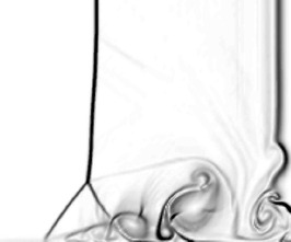
2$\times$

(b) *

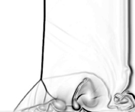
4$\times$

(c) *

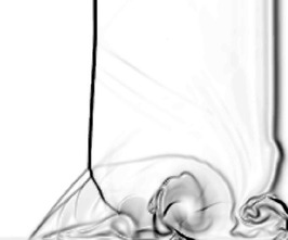
8$\times$

(d) *

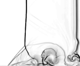
16$\times$

(e) *

Reference

(f) *

Fig. 14: Viscous shock tube: This setup contains simulations of a complex unsteady viscous shock flow [56] with different resolutions. The reference for the user studies was given as the highest resolution result, i.e., the one with the smallest discretization error. Due to the simulated viscosity, the sequence converges towards a result very similar to the ground truth.

The flow solver for this case follows the general eno methodology [26] except that the interpolation is applied with a W5 scheme. Specifically, the Roe approximation is used for the characteristic decomposition at the computational cell faces, the Lax-Friedrichs formulation is used for the numerical fluxes, and the 3rd-order Total Variation Diminishing Runge–Kutta scheme is used for time integration [33]. In this two-dimensional case, the shock wave Mach number is 2.37 [34], the viscosity is assumed to be constant, and the Prandtl number is 0.73, which gives a Reynolds number of 1000 [32]. The simulations are performed on uniform grids of 320$\times$160 (1$\times$), 640$\times$320 (2$\times$), 1280$\times$640 (4$\times$), 2560$\times$1280 (8$\times$), and 5120$\times$2560 (16$\times$). The simulations are visualized with the density gradient sampled on the lowest resolution as shown in Fig. 14, while the reference visualizes the data set of 16$\times$ without down-sampling.

3.2 Double Mach reflection

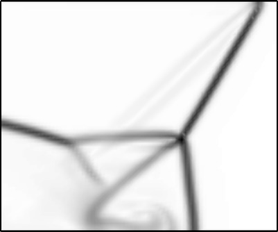
2$\times$

(b) *

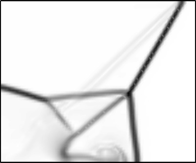
4$\times$

(c) *

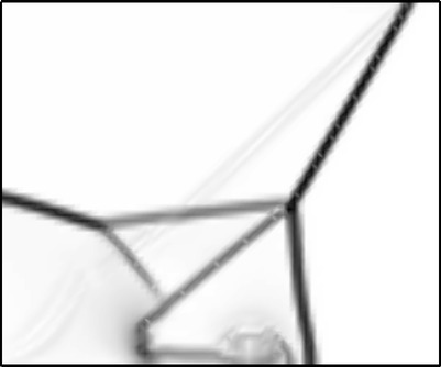
8$\times$

(d) *

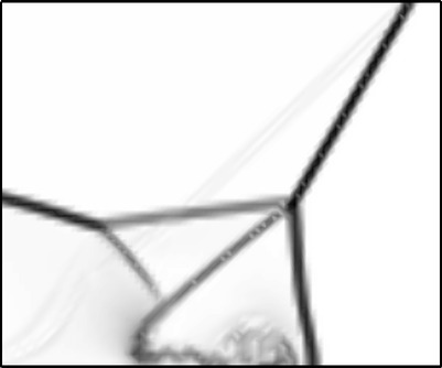
16$\times$

(e) *

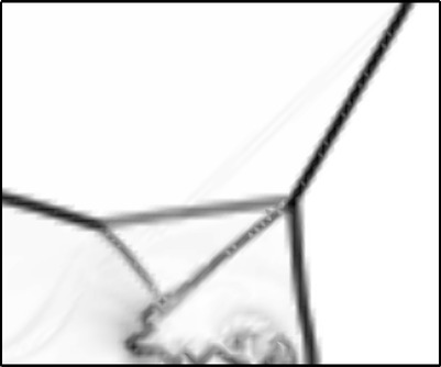
Reference

(f) *

Fig. 15: Double Mach reflection: This setup contains simulations of a two-dimensional inviscid flow with a strong shock [61] with different resolutions. The reference data set was the highest resolution result. Being an inviscid flow problem, this sequence does not exhibit numerical convergence in the traditional sense. Despite this, participants of the corresponding user study had no significant problems establishing the correct ordering.

The underlying flow solver is the same as that for the viscous shock tube above; but, it solves the inviscid Euler equation instead. In this two-dimensional case, a right-moving Mach 10 shock wave is reflected by a horizontal wall with an incidence angle of 60^o [29]. The simulations are done on uniform grids of 240$\times$60 (1$\times$), 480$\times$120 (2$\times$), 960$\times$240 (4$\times$), 1920$\times$480 (8$\times$), and 3840$\times$960 (16$\times$). The simulations are visualized with the density gradient sampled on the lowest resolution, as shown in Fig. 15, while the reference visualizes the data set of 16$\times$ without down-sampling.

3.3 Taylor-Green vortex

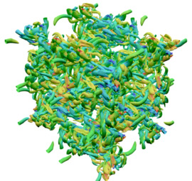
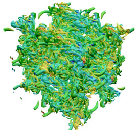
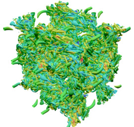
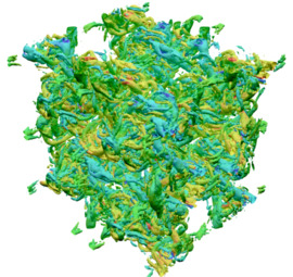
0ptReference 0ptW5 0ptW5z 0ptW6c
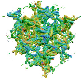
0ptT5 0ptT5o 0ptT6 0ptT6o

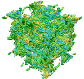
(a) *

(b) *

(c) *

(d) *

(e) *

(f) *

(g) *

(h) *

(i) $256^{3}$

Fig. 21: tgv flow simulations with different resolutions: The images visualize Q-criterion isosurfaces for $Q=3$ and are colored by $x$-component of vorticity.

Although the tgv [35, 36] is a typical incompressible flow problem, the solver used here is the same as above used for simulating compressible flows with shocks, except different eno schemes are applied. Since the Mach number is less than 0.1, the density variations are negligible in this case. The Reynolds number of the problem is 3600. As a consequence, turbulent flow develops shortly after the initial condition. The simulations are carried out in a periodic box on uniform grids of 64³ (1$\times$), 128³ (2$\times$), and 256³ (4$\times$). The reference simulation is done on a grid of 512³ (8$\times$). The simulations are visualized according to the Q-criterion [37] for an isosurface of $Q=3$ and colored with the $x$-component of vorticity as shown in Fig. 21.

Next, we describe the three solver variants that will be used for a more general evaluation of our user study methodology below.

3.4 Breaking dam

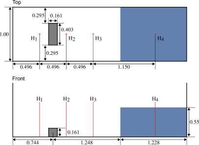
Reference

(b) *

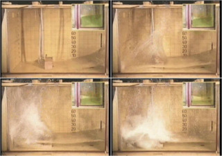
flip (1$\times$)

(c) *

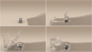
flip (2$\times$)

(d) *

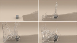
flip (4$\times$)

(e) *

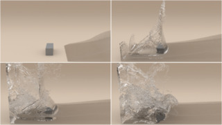
sph (1$\times$)

(f) *

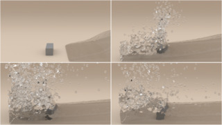
sph (2$\times$)

(g) *

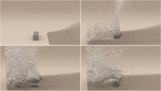
sph (3$\times$)

(h) *

Fig. 8: Breaking dam: The top left shows the specifications of this experimental setup [42]. The probe positions for graphs in Fig. 9 are denoted as H${}_{1\textrm{-}4}$. The reference image (top right) shows four selected frames of a video recorded from the real-world experiment [51]. The images in the bottom two rows show the corresponding frames of simulations from two methods (i.e., flip and sph) with different resolutions. (The resolution multiplier is shown below each image.)

The first of the three setups used to evaluate the robustness of our user studies employs two representative Eulerian and Lagrangian free surface liquid simulation methods: flip [38, 39] and sph [40, 41]. The top left of Fig. 8 shows the simulation setup [42]. flip uses a regular grid of 80$\times$75$\times$25 for (1$\times$), 160$\times$150$\times$50 for (2$\times$), and 320$\times$330$\times$100 for (4$\times$) while sampling each cell using 2³ particles; i.e., each simulation uses 83k, 664k, and 5,315k particles, respectively. Likewise, sph uses 80k Lagrangian particles for (1$\times$), 665k for (2$\times$), and 2,253k for (3$\times$). Both methods simulate this setup with the gravity of 9.8$\mathrm{m}$/$\mathrm{s}$ and without additional viscosity and surface tension. flip uses first-order boundary conditions for the Dirichlet pressure boundary conditions at the free surface and free-slip velocity boundary conditions for solid surfaces. The sph solver is based on the work of [41]. We use the cubic spline kernel for the sph quantities and dummy particles at the wall for boundary conditions of pressure and density.

3.5 Plume

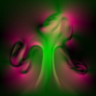
5$\times$

(c) *

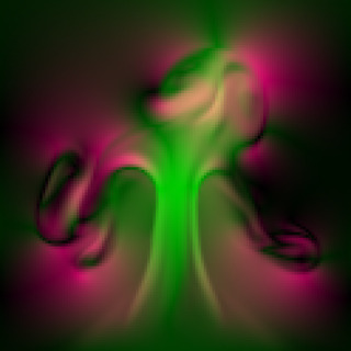
10$\times$

(d) *

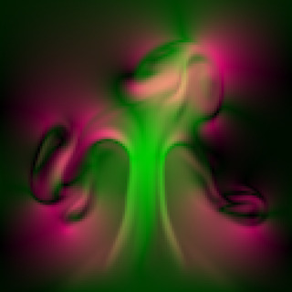
50$\times$

(e) *

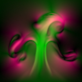
100$\times$

(f) *

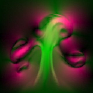
500$\times$

(g) *

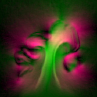
1000$\times$

(h) *

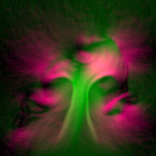
Fig. 10: Rising hot plume: This test compares simulations of a hot plume of gas where each simulation adds different levels of noise with the multiplier shown below each image. The reference data set is the noise-free result, and larger amounts of noise lead to stronger non-linear deviations from the reference. The images visualize the x and y velocity components in purple and green, respectively.

As a second setup, a rising plume setup is simulated with a two-dimensional Eulerian simple solver [43] using a Boussinesq approximation. It employs a marker-and-cell grid [44] in conjunction with the fractional step method [45] and Chorin projection [46]. The computational grid has a resolution of $128^{2}$ quadratic cells, and the variance shown in the visualizations of Fig. 10 is generated by adding differently scaled white noise to both components of the velocity. The lowest amount for the version denoted by 1$\times$ uses random values in the range of [0, 10^-4]. A buoyancy force of $10^{-3}$ per timestep is employed, and, due to the transient nature of the simulation, a snapshot after 100 timesteps is visualized. In the visualizations, noise levels of 5$\times$ and 1$\times$ lead to barely visible changes, which, nonetheless, influenced the mean assessments of participants in the corresponding user study.

3.6 Airfoil

Lastly, we simulate a steady-state flow around an airfoil. This data set is likewise simulated with simple solver [43], but, in this case, an irregular triangle mesh with 42,730 nodes and 126,964 elements was used for the computational grid. The simulation is solved for Reynolds-average steady-state and employs the Spalart-Allmaras one equation turbulence model [47] with a kinematic viscosity $\nu$ of 10^-5. Angles of attack vary for a freestream velocity magnitude $|\vec{v}_{\text{free}}|$ of 85, yielding an average Reynolds number $Re$ of 4.25 million across the simulated variants. The airfoil uses the profile GOE-633 obtained from the UIUC database [48].

The visualization for pressure uses the perceptually linear color profile “magma”, while the two velocity components intentionally use a regular color profile “jet”. Our results show that the latter does not pose problems for our hvs-based evaluation.

4 Results and discussion

We establish the effectiveness of the hvs as a means of accuracy evaluation for numerical simulations through a series of user studies. Our user studies employ the 2afc methodology outlined above, in which participants are asked which of two candidates they consider to be closer to a third candidate shown as reference. Each of these candidates typically consists of field data obtained with one of the numerical methods outlined above. For a data set comparing different candidates, each participant answers all pairwise questions twice in a user study where the alternatives for each question are shown in random spacial order. All of our user studies were performed with 50 participants per study, which we have found to be sufficient for robust assessments with low variance. Overall, we collected 56,300 answers of 567 different participants from 55 countries via crowdsourcing.

Due to the simplicity of each task, these studies are very easy to set up and incur only a small cost. In our setup for a study with six evaluation candidates, the cost was 33,- USD. In addition, our study results were very robust. Based on the repeated questions, we measured reliability by computing the matching rate of answers, which was 83% on average for all studies in Experiment 1. Moreover, we evaluated three different crowdsourcing platforms and found that their results for the same data set are very consistent. Here, the correlations of the results from different platforms were all greater than 0.95 ($P<0.001$).

4.1 Experiment 1: hvs as evaluation metric

It is widely acknowledged that the hvs performs extremely well at finding the similarities and differences between two images [16, 17]. This property naturally motivates employing it for quality assessments of typical image processing tasks such as compression and synthesis [14]. Our experiments demonstrate that hvs-based evaluations can correctly recover the ground truth ranks for a broad range of simulation cases and visualization types as shown in Fig. 2. We have investigated a breaking dam case with a more realistic depiction in addition to four test cases with more abstract scientific visualizations. These visualizations cover a wide variety of simulation types and include a rising hot plume shown in terms of vorticity, a turbulence simulation around an airfoil visualized with pressure and velocity profiles, and density visualizations of shock tube simulations. Whereas participants had a good intuition for the phenomena shown in the breaking dam scene, we expect the large majority of the participants to have no understanding of the underlying physics for these four cases [49]. Our results show that all studies reliably recover the ground truth ordering for all eight scenarios even for cases with abstract imagery as shown in Fig. 3. Thus, such crowd-sourced evaluations of scientific data pose a reliable way to evaluate sets of scientific results.

Breaking dam

(a) *

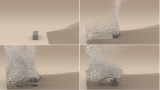
Plume

(b) *

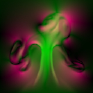
Airfoil

(c) *

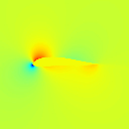
Viscous shock

(d) *

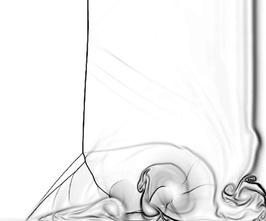
Double Mach reflection

(e) *

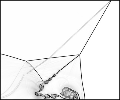
Fig. 2: A selection of fluid simulation evaluations: The images show the visualized simulation results where a control parameter such as resolution or velocity boundary condition is modified in increments to yield a sequence with known ordering. Simulation setups and visualizations for each case differ substantially. The full data sets for each example are shown in Fig. 8 and 10–15, respectively.

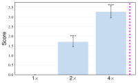
(a) Breaking dam with flip

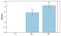
(b) Breaking dam with sph

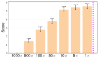
(c) Plume

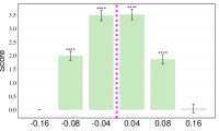
(d) Airfoil (pressure)

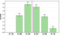
(e) Airfoil (x-velocity)

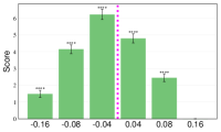
(f) Airfoil (y-velocity)

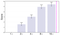
(g) Viscous shock

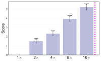
(h) Double Mach reflection

Fig. 3: Accuracy evaluations for the different simulation setups shown in Fig. 2: The dashed magenta line indicates the baseline for each evaluation. Thus, we anticipate that the performance score of a simulation is higher if it is closer to the baseline. The participants of each study recover the ground truth ordering without any errors in the established ranks. ***$P<0.001$ and ****$P<0.0001$.

Due to its highly non-linear behavior, it is extremely difficult to predict how a small change of a parameter affects the result of a flow simulation. Nevertheless, the results will differ more strongly from a baseline result for larger variations of that parameter. For example, if we simulate a certain setup using different resolutions considering the highest resolution as the baseline (i.e., ground truth), the lowest resolution will differ most from the baseline due to the largest accumulated numerical errors. We conduct a series of user studies from five different examples where we know the true rank due to controlled parameter changes. Due to the changed parameters, the calculated solutions differ in a variety of ways; for example, they contain shifted velocity structures, varying vortices locations, and different configurations of transported passive quantities. We chose a representative set of typically evaluated physical variables, such as density and velocity, which were visualized either realistically or according to common practice in the respective scientific community.

Fig. 3 summarizes the resulting ranks of the visualized data sets with respect to their similarity to a chosen ground truth data set. Here, the dashed magenta line indicates the location of this ground truth in each parameter space. Thus, the distance to the dashed line directly indicates the similarity of the solutions, and the monotonically increasing scores towards the magenta lines show that all studies recover the expected ordering. As a consequence, all studies yield a Kendall rank correlation coefficient [50] of one against the ground truth ranks.

As a first real-world validation case, we consider a breaking dam setup, which contains a large scale wave and splash forming in a rectangular container. The breaking dam represents a widely adopted simulation case for free surface flow simulations [51]. We simulate this case with two representative methods, i.e., sph [41] and flip [39] solvers, using three different resolutions per method. For this simulation, we compare four frames from a realistic visualization of the water surface as shown in Fig. 8 with the corresponding video frames of the real-world experiment.

Traditionally, the accuracy of a simulation for this breaking dam setup evaluated with four point-wise probe measurements. However, this data is highly inconclusive for the simulation data under consideration. The rmse between the experiment and simulation data is shown in Table 1. This result is even more pronounced when considering the experimental video and the simulation visualizations for comparisons. Although improved metrics such as the psnr [52] and the ssim [53] have been proposed as specialized tools for comparing images, the substantially different content of the real-world images and visualizations yields quantified differences that are as inconclusive as the rmse values above as shown in Table 1. In contrast, our hvs-based evaluation methodology is able to successfully recover the resolution-based ordering of this breaking dam case for both simulation methods as shown in Fig. 3(a) and Fig. 3(b).

Method	H1	H2	H3	H4	psnr	ssim
flip (1$\times$)	0.091	0.036	0.042	0.044	14.179	0.617
flip (2$\times$)	0.098	0.044	0.031	0.028	14.100	0.606
flip (4$\times$)	0.108	0.045	0.020	0.026	14.024	0.590
sph (1$\times$)	0.186	0.024	0.023	0.023	14.021	0.581
sph (2$\times$)	0.129	0.032	0.025	0.026	13.994	0.574
sph (3$\times$)	0.168	0.043	0.025	0.021	13.860	0.570

Table 1: rmse, psnr, and ssim of breaking dam simulations: The rmse is computed using the experimental data and corresponding simulation values at four probe positions, H_1-4. The psnr and ssim are computed between the real-world image and visualization of each simulation. Underlined bold numbers indicate the best performance for each of the two methods per column.

Beyond the breaking dam case, we also examine a variety of simulations where the target images are more abstract scientific visualizations. The four additional simulation cases in Fig. 2 include a rising hot plume shown in terms of vorticity, pressure and velocity profiles around an airfoil from a Reynolds-averaged Navier-Stokes turbulence simulation, and density gradient magnitudes for viscous shock tube and double Mach reflection setups shown in grayscale, respectively. Whereas participants will have had a good intuition for the phenomena shown in the breaking dam scene, we expect the large majority of the participants to have no understanding of the underlying physics for these four cases [49].

For the rising plume setup of Fig. 2, we consider different levels of synthetic noise added to the fluid velocity fields. This represents a controlled form of artificial error mimicking effects of numerical viscosity. The ground truth rank with respect to the level of introduced noise is recovered by participants, and it is noticeable that the curve flattens for noise levels of 5$\times$ and 1$\times$. These noise levels lead to very slight changes in the simulated fluid motion and are difficult to discern. Despite being barely noticeable, the participants, by sake of large numbers, recovered the right ordering of the different simulation results.

The studies of Fig. 3(d)–3(f) show results for user study evaluations performed with different variables of a classic airfoil flow simulation. Here, the target ranks are established from different angles of attack with a zero-degree centerline being used as reference. Hence, the dashed magenta lines in these graphs are located in the middle, and the graphs show monotonically increasing scores towards this centerline. The two shock studies in Fig. 2 vary simulation resolutions for a viscous and an inviscid shock dynamics problems. The latter one is especially interesting as it represents an inviscid flow problem that does not have numerical convergence in the traditional sense. In both cases, our hvs-based evaluations recover the ordering with respect to simulation resolution.

4.2 Experiment 2: Discretization schemes and features

Having demonstrated the robustness of the hvs-based evaluation methodology, we now turn to analyzing the accuracy of a set of numerical discretization schemes in the context of two important test cases. More specifically, we consider seven representative methods of finite difference discretizations from the class of eno schemes. These schemes are very widely used and form the basis of a vast number of methods for partial differential equation solvers. As such, comparisons of these methods, in order to establish which methods to choose for certain applications, have received a significant amount of attention but have often remained inconclusive [54, 55]. In contrast to these studies, our crowd-sourced evaluations manage to uncover clear differences between the methods and yield insights that some of the newer schemes under consideration do not give a stable performance. Our studies illustrate how the user study methodology can be leveraged to measure the accuracy of simulation methods (Fig. 4). For these eno schemes, it yields an objective and robust evaluation for a class of methods that have been discussed controversially in the scientific community.

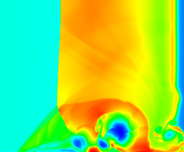
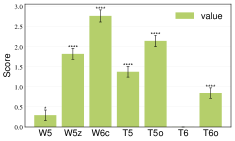
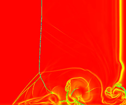
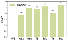
Fig. 4: Visualizations of a viscous shock tube simulation and performance evaluations of seven finite difference schemes for each visualization: The left side shows absolute density values, while the right side visualizes the density gradient. ****$P<0.0001$ and *$P<0.05$.

Here, we present our evaluation results for seven representative methods of finite difference discretizations from the class of eno schemes. We focus on methods of fifth and sixth order as these represent the most commonly used compromise between performance and accuracy. In our study, we included three weighted eno schemes: W5, W5z, and W6c. Although the W5 scheme does not represent the latest state of the art, it was included as a traditional variant for comparison. In addition, we included four more recent modified schemes, so-called targeted eno schemes, denoted as T5, T5o, T6, and T6o. Here, 5 and 6 in each of the abbreviations indicate the order of the scheme, and the “z”, “c”, or “o” suffixes indicate different variants.

We evaluate these schemes with respect to their performance in compressible flow solvers for a viscous shock tube simulation [56, 57]. This setup represents a fundamental experiment for engines and turbines and, as such, has been widely studied in simulations. The central quantity in these simulations is the fluid density, which is important in terms of its overall magnitude and with respect to its gradients. While the former highlights the density values of larger regions, the gradient emphasizes the position of shock waves and contact discontinuities.

Hence, in order to analyze both aspects, we visualized the data sets simulated with each of the seven schemes twice: once using absolute values and once using the density gradient, each time employing the established way to visualize the corresponding data (Fig. 4). To generate a reference data set, we used a high-resolution simulation with the traditional W5 scheme. The ranks for all schemes of both studies are shown in Fig. 4.

When considering the accuracy of the density gradient, all schemes clearly outperform the W5 baseline. This is not surprising as W5 is the oldest scheme of the set and many of the other schemes were specifically developed as an improvement of it. However, interestingly, the higher order T6 scheme performs less well than its fifth-order counterparts.

Turning to the accuracy for absolute densities shown in Fig. 4 left, the differences in performance are significantly more diverse than for the density gradients. The W6c scheme clearly outperforms all other schemes, and the class of targeted schemes stays behind the two improved weighted variants (i.e., W5z and W6c). The T6 scheme, in particular, is identified as deviating strongly from the reference solution and performs even worse than the W5 baseline.

4.3 Experiment 3: Localization

We additionally demonstrate that our methodology can be applied recursively in a divide-and-conquer fashion to deduce which parts of the data were discriminative. Starting with a user study evaluation for a chosen number of full data sets, we perform the evaluation on identical smaller regions of each data set. We can then correlate the ranks for the localized data set with the ranks for the whole data set. These localized evaluations naturally force participants to evaluate the data with respect to subsets of the data and, in this way, can localize differences in the results.

Regarding the evaluations discussed so far, there is an important yet challenging open question: Which parts of a solution led to its assessment as accurate or inaccurate? This is especially important when using such evaluations to guide future developments rather than for making discrete decisions. In order to improve a method that produced one of the evaluated solutions, it is important to localize regions that were discriminative.

While, in general, a stochastic subdivision with overlapping regions would be ideal, we have found that a simple $2\times 2$ subdivision yields excellent results, i.e., our subdivision scheme follows a quadtree structure. To localize discriminative regions in the data, we can first compute a reliability factor for the participant’s answers. With our user study methodology, a participant sees every data pair twice. From these duplicate questions, we can compute a fraction of matching answers for a given data pair. In the limit of random answers, i.e., 50% of votes for each of the two alternatives, we can conclude that participants were not able to distinguish the two corresponding visualizations.

Let $I$ be an original image, then $I_{i}$ represents a cutaway patch of $I$ where the subscript $i$ denotes a single quadrant. Successively appended subscripts denote the children of a node; for example, $I_{ij}$ represents a cutaway quadrant $j$ of a larger cutaway patch $I_{i}$.

We start with four quadrants of the image set $I^{\mathrm{dv}}$ where the superscript “dv” denotes the density value visualization of Fig. 16(i). The set of independent user studies for each quadrant reveals that two upper quadrants $I_{1}^{\mathrm{dv}}$ and $I_{2}^{\mathrm{dv}}$ are less distinguishable. This is intuitively evident as they contain very few detailed structures. Their average matching rates of answers were 51.62% ($\sigma$=7.29%) and 51.71% ($\sigma$=9.29%), respectively. Note that the matching rates for the two lower quadrants $I_{3}^{\mathrm{dv}}$ and $I_{4}^{\mathrm{dv}}$ were 86.38% ($\sigma$=12.42%) and 63.71% ($\sigma$=5.57%), respectively. The high matching rate implies that the participants consistently observe the differences of two patches over the whole set of questions.

On the other hand, if a region results in high reliability and exhibits results that correlate with the evaluation for the whole data, it strongly indicates that this region led to the original assessment. For the two lower quadrants of the viscous shock tube example, we compute the correlation coefficient $\rho$ for their results against the evaluations of the whole data set, i.e., the original visualization. From the density value studies, we found a strong positive correlation between the lower left part $I_{3}^{\mathrm{dv}}$ and the whole $I^{\mathrm{dv}}$, i.e., $\rho(I^{\mathrm{dv}},I_{3}^{\mathrm{dv}})=0.958$ $(P<0.001)$. In contrast, the lower right part $I_{4}^{\mathrm{dv}}$ is less correlated to the whole $I^{\mathrm{dv}}$, i.e., $\rho(I^{\mathrm{dv}},I_{4}^{\mathrm{dv}})=0.847$ $(P<0.05)$. Drilling down, we also found the strong positive correlations within the part $I_{3}^{\mathrm{dv}}$, i.e., $\rho(I^{\mathrm{dv}},I_{33}^{\mathrm{dv}})=0.979$ $(P<0.001)$, $\rho(I^{\mathrm{dv}},I_{34}^{\mathrm{dv}})=0.98$ $(P<0.001)$, and $\rho(I_{33}^{\mathrm{dv}},I_{34}^{\mathrm{dv}})=0.996$ $(P<0.00001)$. This indicates that the part $I_{3}^{\mathrm{dv}}$ (and particularly, $I_{33}^{\mathrm{dv}}\cup I_{34}^{\mathrm{dv}}$) is very influential for the evaluation of the whole simulations.

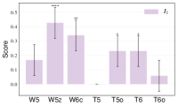
$I^{\mathrm{dv}}_{2}$

(b) *

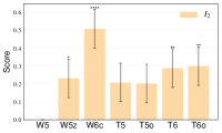
$I^{\mathrm{dv}}_{3}$

(c) *

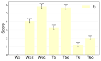
$I^{\mathrm{dv}}_{4}$

(d) *

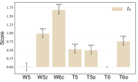
$I^{\mathrm{gd}}_{1}$

(e) *

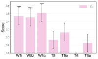
$I^{\mathrm{gd}}_{2}$

(f) *

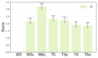
$I^{\mathrm{gd}}_{3}$

(g) *

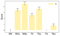
$I^{\mathrm{gd}}_{4}$

(h) *

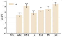
$I^{\mathrm{dv}}_{33}$

(i) *

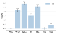
$I^{\mathrm{dv}}_{34}$

(j) *

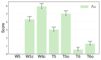
$I^{\mathrm{gd}}_{33}$

(k) *

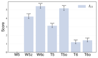
$I^{\mathrm{gd}}_{34}$

(l) *

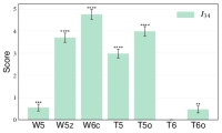
Fig. 18: User study results for the error localization (Experiment 3): The graphs show the performance scores of seven discretization schemes for the cutout regions of the viscous shock tube simulations. The superscripts “dv” and “gd” represent the density value visualizations (Fig. 16(i)) and gradient visualizations (Fig. 16(r)), respectively. The subscripts indicate each region according to Fig. 17. ****$P<0.0001$, **$P<0.01$, *$P<0.05.$

Applying our analysis recursively to the lower left quadrant, we can identify both of its bottom sub-quadrants as discriminative regions. This region primarily exhibits shock-boundary layer interactions near the bottom wall of the shock tube. Surprisingly, the key feature that distinguishes the shock tube data is not the large separation vortex near the bottom center of the visualizations. Despite this vortex being the most salient feature at first sight, the participants have identified the lower left “$\lambda$-shock” region as a key difference in the data set, and a post-mortem analysis of the visualizations confirms this assessment. One of the two sub-quadrants is shown in Fig. 5 for two representative schemes. The performance evaluation results of this experiment are summarized in Fig. 18.

Target area

(a) *

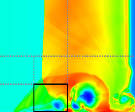
W6c

(b) *

T6

(c) *

Reference

(d) *

Fig. 5: Localization: For the highlighted target area, the best (W6c) and worst (T6) scoring schemes are shown. The T6 solution clearly deviates from the reference (shown right).

4.4 Experiment 4: Consistency

One of the most pressing questions for any practitioner in the field of numerical simulations is to know how reliable and accurate the solution of a given implementation, method, or solver is. The most common way to study the behavior of a method is in terms of its convergence order under refinement. It is usually expressed as the order of the polynomial for the limiting behavior of the approximation error with respect to the step size. While this expression reliably indicates the behavior as the step size approaches zero, it hides the constant factors for the polynomial terms, which are typically unknown and problem dependent. In practice, it is also often difficult to mathematically prove the order of convergence for a full algorithm, and, as a consequence, it is often computed with a series of measurements for a chosen test case. These measurements again rely on direct vector norms and thus inherently require smooth and converged solutions [15].

For a solution outside of the convergence regime, i.e., with a finite step size, the order of convergence does not guarantee that a higher order method actually performs better than one with lower order. However, with the user study methodology outlined above, we have a measure of relative accuracy for these unconverged regimes, and it allows us to establish the notion of a ncm, which we will abbreviate as ncm in the following. We define this quantity as the consistency of a method’s performance. If a method repeatedly achieves a high score and outperforms its competitors, this will be reflected in a small ncm. As a consequence, the method also has the highest chance to perform well when applied to similar new problems. It is worth pointing out that while our approach is the first one to establish this consistency in regimes that are not fully converged, just like traditional tools, it does not guarantee the same evaluation results for new applications. However, if those applications fall into a similar regime as the one where the evaluation was performed, there is very high likelihood that the results are more conclusive than the results of regular convergence studies.

To compute the ncm, we employ the winning probability. Intuitively, the winning probability represents the average probability of one method performing better than the others. The standard deviation of the winning probability across a series of studies, then, indicates how consistently a method behaves relative to the others and yields the ncm. Thus, the method with the smallest ncm is the one with the lowest standard deviation in terms of winning probability.

We have measured the ncm for the aforementioned eno schemes in two very different simulation settings: first in the context of incompressible turbulence and second in the context of compressible shocks. We consider the incompressible case with three-dimensional Navier-Stokes simulations of tgv problem [35] with a Reynolds number of 3,600 [36] that leads to complex decaying vortex structures as shown in Fig. 6. The compressible case is studied with a set of two-dimensional shock tube simulations, similar to those shown in Fig. 4. Each test case represents an important regime of fluid flow problems, and our evaluations successfully establish the consistency of the different simulation methods across a range of different resolutions.

1$\times$

(a) *

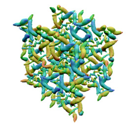
2$\times$

(b) *

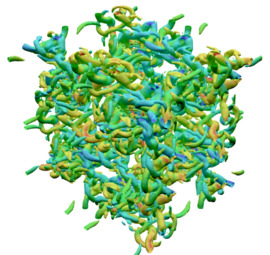
4$\times$

(c) *

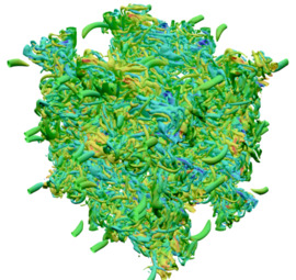
Reference

(d) *

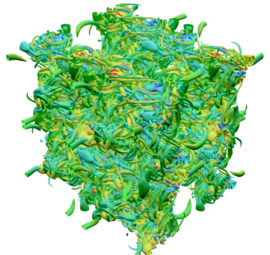
Mean winning probability

(e) *

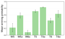
Fig. 6: Different resolutions of the Taylor-Green vortex flow simulation: The resolutions are 64³ for 1$\times$, 128³ for 2$\times$, 256³ for 4$\times$, and 512³ for Reference. The images show the isosurface for a Q-criterion value of three and are colored by x vorticity magnitude. The graph shows mean and standard deviation of winning probabilities for seven schemes across these resolutions.

Interestingly, we find that the method that performs worst for the incompressible case emerges as the winner for the compressible shock flows. These results do not contradict each other; they rather illustrate how the complex interplay of choices for numerical solvers can influence the final results. Obviously, the assessment of this method would have been meaningless in isolation, and it requires a robust assessment of its accuracy in practical settings to reveal this behavior. Since both setups represent typical computational fluid dynamics solvers and resolution ranges, our studies highlight the importance of accuracy measurements in the near-convergence regimes, where methods are typically used in practice rather than in the fully converged limit.

Fig. 6 shows a selection of tgv simulation results with increasing resolution together with the reference solution that was obtained numerically with a high-resolution simulation. We evaluated each scheme at three different resolutions, and the corresponding winning probabilities are shown in the figure together. (See also Table 2.) It is immediately apparent from the graphs that some of the schemes, such as T6o and W5z, exhibit significant differences across the three resolutions. The T5o scheme, on the other hand, has a very high and consistent winning probability. Thus, T5o is the clear winner among the investigated schemes, while the W6c scheme performs worst despite its high order.

We also performed an ncm study with an even wider range of resolutions for the viscous shock tube case from Experiment 2. Here, we used five different resolutions, which are shown in Fig. 7 together with their winning probabilities. While T5o has the highest mean of winning probabilities for these simulations, it also exhibits a very high standard deviation. Thus, it is very unreliable in terms of its performance for viscous shock tube simulations. In this case, the W6c scheme has the lowest standard deviation and thus emerges as the best candidate among the investigated schemes.

1$\times$

(a) *

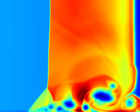
1.5$\times$

(b) *

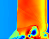
2$\times$

(c) *

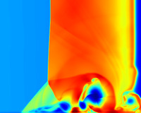
3$\times$

(d) *

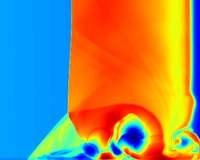
4$\times$

(e) *

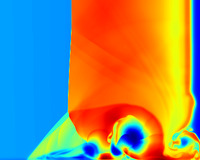
Reference

(f) *

Mean winning probability

(g) *

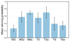
Fig. 7: Resolutions used to determine the ncm for viscous shock tube simulations: From left to right, 1$\times$=640$\times$320, 1.5$\times$=960$\times$640, 2$\times$=1280$\times$640, 3$\times$=1920$\times$960, 4$\times$=2560$\times$1280, and Reference is 5120$\times$2560. The graph shows mean and standard deviation of winning probabilities for seven schemes across these resolutions.

5 Conclusion and outlook

We have shown that the hvs provides a reliable and robust new evaluation metric that can be employed to analyze a wide range of previously inconclusive problems. Furthermore, we have shown its usefulness to quantify and measure a derived property, namely the near-convergence consistency.

However, our study only represents a first step towards establishing perceptual evaluations as an accuracy metric. As such, our approach has limitations that point towards avenues of future work. For example, for the evaluations of this study, we have relied on established visualization techniques for the respective fields our model problems were selected from. This has naturally imposed knowledge from domain experts. However, it will be highly interesting to further investigate the influence of visualization on reliability and robustness of our approach. Moreover, whereas the experiments of this study have focused on fluid dynamics problems, we envision that this evaluation methodology will be preferable over simple vector norms for any other problem with complex field data, such as meteorology and solid mechanics [58, 59, 60].

Table 2: Winning probability for Taylor-Green vortex flow simulations (top) and viscous shock tube simulations (bottom): $\mu$ and $\varepsilon$ represent the average index and standard deviation (i.e., the ncm), respectively. The underlined bold number indicates the highest probability or lowest error thus the best performance at each column, and the bold number indicates the second best one.

Method 1$\times$ 2$\times$ 4$\times$ $\mu$ $\varepsilon$ W5 .130 .142 .397 .223 .151 W5z .478 .615 .662 .585 .095 W6c .163 .075 .020 .086 .072 T5 .710 .665 .757 .711 .046 T5o .813 .847 .827 .829 .017 T6 .477 .488 .340 .435 .082 T6o .728 .668 .498 .632 .119

Method 1$\times$ 1.5$\times$ 2$\times$ 3$\times$ 4$\times$ $\mu$ $\varepsilon$ W5 .127 .290 .397 .262 .212 .257 .100 W5z .300 .638 .645 .570 .715 .574 .161 W6c .717 .675 .640 .635 .788 .691 .063 T5 .422 .790 .465 .605 .470 .550 .151 T5o .863 .750 .790 .680 .410 .699 .174 T6 .635 .158 .235 .480 .420 .386 .191 T6o .437 .198 .328 .268 .485 .343 .118

Appendix

Specifications [$\mathrm{m}$]

(a) *

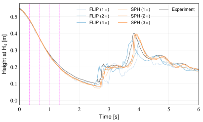
Fig. 9: Graphs for the breaking dam user study: The graphs plot the water height values measured at four probes, H${}_{1\textrm{-}4}$, from both the experiment (black) and simulations (blue and orange). The dashed vertical lines in magenta indicate the selected moments for the images shown in Fig. 8. It is difficult to clearly determine which simulation performs better (i.e., closer to the black ground truth) from these graphs.

Reference

(a) *

1$\times$

(b) *

0ptReference ($a=0$)
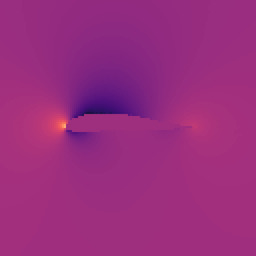
0pt$a=-0.16$

(a) *

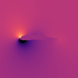
(b) *

0pt$a=-0.08$

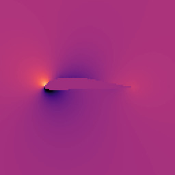
(c) *

0pt$a=-0.04$

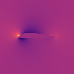
(d) *

0pt$a=0.04$

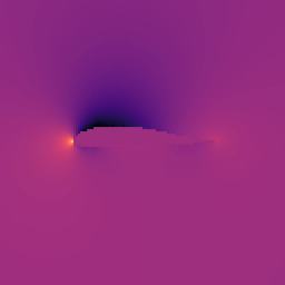
(e) *

0pt$a=0.08$

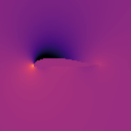
(f) *

0pt$a=0.16$

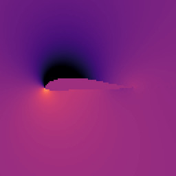
(g) *

(h) Pressure

0ptReference ($a=0$)
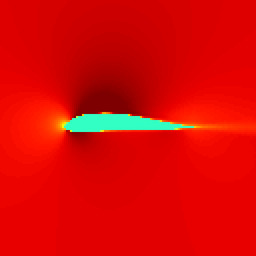
0pt$a=-0.16$

(a) *

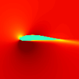
(b) *

0pt$a=-0.08$

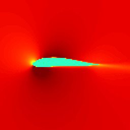
(c) *

0pt$a=-0.04$

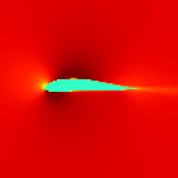
(d) *

0pt$a=0.04$

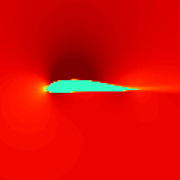
(e) *

0pt$a=0.08$

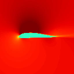
(f) *

0pt$a=0.16$

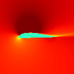
(g) *

(h) X-velocity

0ptReference ($a=0$)
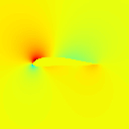
0pt$a=-0.16$

(a) *

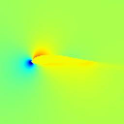
(b) *

0pt$a=-0.08$

(c) *

0pt$a=-0.04$

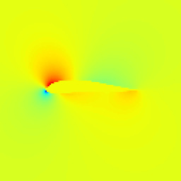
(d) *

0pt$a=0.04$

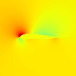
(e) *

0pt$a=0.08$

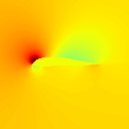
(f) *

0pt$a=0.16$

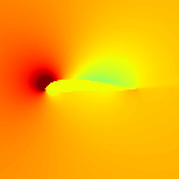
(g) *

(h) Y-velocity

Fig. 13: Airfoil Reynolds-averaged Navier-Stokes turbulence: An airfoil profile is simulated in two dimensions for different angles of attack (given as $a$ in radians below each image). These visualizations show the pressure distribution around the airfoil and the x and y components of the flow velocity (from top to bottom). In this case, the zero angle, $a=0$, is given as reference data set in the user studies.

1$\times$

(a) *

1$\times$

(a) *

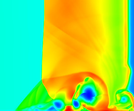
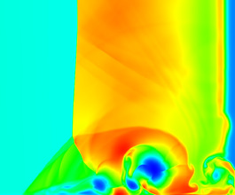
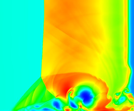
0ptReference 0ptW5 0ptW5z 0ptW6c
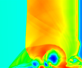
0ptT5 0ptT5o 0ptT6 0ptT6o

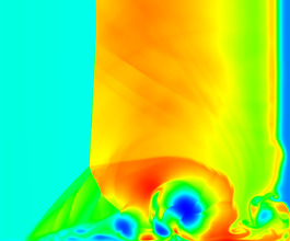
(a) *

(b) *

(c) *

(d) *

(e) *

(f) *

(g) *

(h) *

(i) Density value

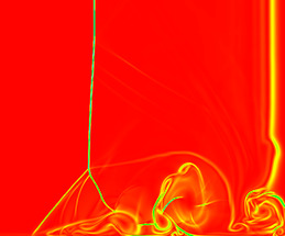
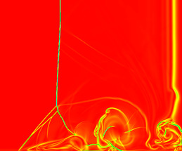
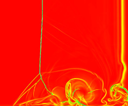
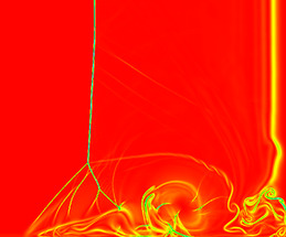
0ptReference 0ptW5 0ptW5z 0ptW6c
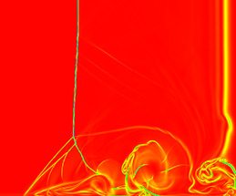
0ptT5 0ptT5o 0ptT6 0ptT6o

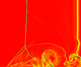
(j) *

(k) *

(l) *

(m) *

(n) *

(o) *

(p) *

(q) *

(r) Density gradient

Fig. 16: Viscous shock tubes simulated with different discretization schemes: The images (16(i)) and (16(r)) show visualizations of the density value and the density gradient of each solution, respectively. The grid resolutions are 5120$\times$2560 for the reference and 1280$\times$640 for the different eno schemes.

(a) Quadtree structure

0pt$I^{\mathrm{dv}}_{1}$

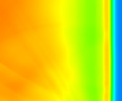
(b) *

0pt$I^{\mathrm{dv}}_{2}$

(c) *

0pt$I^{\mathrm{dv}}_{3}$

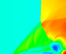
(d) *

0pt$I^{\mathrm{dv}}_{4}$

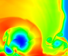
(e) *

(f) Regions of the density value visualization in Fig. 16(i)

0pt$I^{\mathrm{gd}}_{1}$

(g) *

0pt$I^{\mathrm{gd}}_{2}$

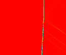
(h) *

0pt$I^{\mathrm{gd}}_{3}$

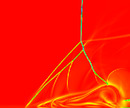
(i) *

0pt$I^{\mathrm{gd}}_{4}$

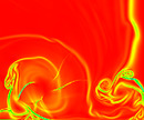
(j) *

(k) Regions of the density gradient visualization in Fig. 16(r)

0pt$I^{\mathrm{dv}}_{33}$

(l) *

0pt$I^{\mathrm{dv}}_{34}$

(m) *

0pt$I^{\mathrm{gd}}_{33}$

(n) *

0pt$I^{\mathrm{gd}}_{34}$

(o) *

(p) Two bottom regions of $I^{\mathrm{dv}}_{3}$ (left) and $I^{\mathrm{gd}}_{3}$ (right)

Fig. 17: Quadtree-based localization: From the root level $I$, the hierarchical subdivisions are denoted with subscripts according to the quadtree structure shown in (17(a)). The figures of (17(f)), (17(k)), and (17(p)) show examples of the localization for the reference data sets of the viscous shock tube simulations in Fig. 16. The superscripts “dv” and “gd” represent the density value visualization (Fig. 16(i)) and gradient visualization (Fig. 16(r)), respectively.

$I^{\mathrm{dv}}_{1}$

(a) *

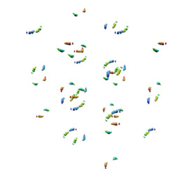
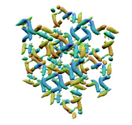
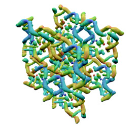
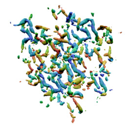
0ptReference 0ptW5 0ptW5z 0ptW6c
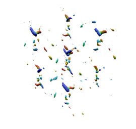
0ptT5 0ptT5o 0ptT6 0ptT6o

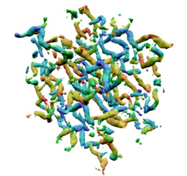
(a) *

(b) *

(c) *

(d) *

(e) *

(f) *

(g) *

(h) *

(i) $64^{3}$

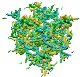
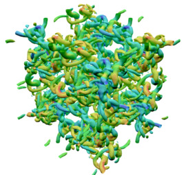
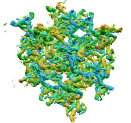
0ptReference 0ptW5 0ptW5z 0ptW6c
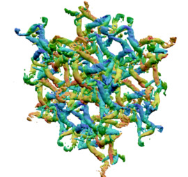
0ptT5 0ptT5o 0ptT6 0ptT6o

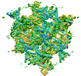
(a) *

(b) *

(c) *

(d) *

(e) *

(f) *

(g) *

(h) *

(i) $128^{3}$

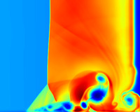
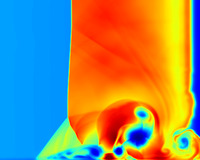
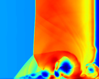
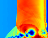
0ptReference 0ptW5 0ptW5z 0ptW6c
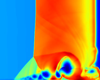
0ptT5 0ptT5o 0ptT6 0ptT6o

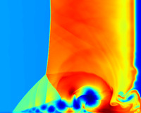
(a) *

(b) *

(c) *

(d) *

(e) *

(f) *

(g) *

(h) *

(i) $640\times 320$

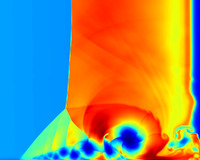
0ptReference 0ptW5 0ptW5z 0ptW6c
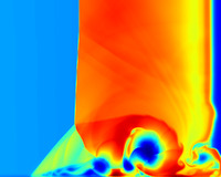
0ptT5 0ptT5o 0ptT6 0ptT6o

(a) *

(b) *

(c) *

(d) *

(e) *

(f) *

(g) *

(h) *

(i) $960\times 480$

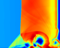
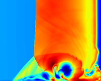
0ptReference 0ptW5 0ptW5z 0ptW6c
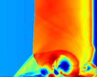
0ptT5 0ptT5o 0ptT6 0ptT6o

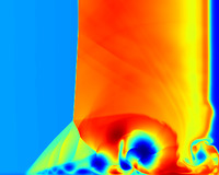
(a) *

(b) *

(c) *

(d) *

(e) *

(f) *

(g) *

(h) *

(i) $1280\times 640$

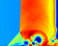
0ptReference 0ptW5 0ptW5z 0ptW6c
0ptT5 0ptT5o 0ptT6 0ptT6o

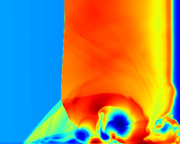
(a) *

(b) *

(c) *

(d) *

(e) *

(f) *

(g) *

(h) *

(i) $1920\times 960$

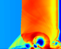
0ptReference 0ptW5 0ptW5z 0ptW6c
0ptT5 0ptT5o 0ptT6 0ptT6o

(a) *

(b) *

(c) *

(d) *

(e) *

(f) *

(g) *

(h) *

(i) $2560\times 1280$

Fig. 26: Viscous shock tube simulations using different discretization schemes with different resolutions: The resolution of the reference data set is 5120$\times$2560.

References

- Montecinos et al. [2012] G. Montecinos, C. Castro, M. Dumbser, E. Toro, Comparison of solvers for the generalized riemann problem for hyperbolic systems with source terms, Journal of Computational Physics 231 (2012) 6472–6494.
- Johnsen and Larsson [2011] E. Johnsen, J. Larsson, Numerical errors generated by WENO-based interface-capturing schemes in multifluid computations, in: 20th AIAA Computational Fluid Dynamics Conference, American Institute of Aeronautics and Astronautics, 2011. doi:10.2514/6.2011-3684.
- Peshkov et al. [2019] I. Peshkov, W. Boscheri, R. Loubère, E. Romenski, M. Dumbser, Theoretical and numerical comparison of hyperelastic and hypoelastic formulations for Eulerian non-linear elastoplasticity, Journal of Computational Physics 387 (2019) 481–521.
- Zhao et al. [2019] G. Zhao, M. Sun, A. Memmolo, S. Pirozzoli, A general framework for the evaluation of shock-capturing schemes, Journal of Computational Physics 376 (2019) 924–936.
- Christie et al. [2005] M. A. Christie, J. Glimm, J. W. Grove, D. M. Higdon, D. H. Sharp, M. M. Wood-Schultz, Error analysis and simulations of complex phenomena, Los Alamos Science 29 (2005) 6–25.
- Press et al. [2007] W. H. Press, S. A. Teukolsky, W. T. Vetterling, B. P. Flannery, Numerical Recipes 3rd Edition, 3 ed., Cambridge University Press, 2007.
- Kat and Els [2012] C.-J. Kat, P. S. Els, Validation metric based on relative error, Mathematical and Computer Modelling of Dynamical Systems 18 (2012) 487–520.
- Oberkampf et al. [2004] W. L. Oberkampf, T. G. Trucano, C. Hirsch, Verification, validation, and predictive capability in computational engineering and physics, Applied Mechanics Reviews 57 (2004) 345–384.
- Rhie and Chow [1983] C. Rhie, W. L. Chow, Numerical study of the turbulent flow past an airfoil with trailing edge separation, AIAA journal 21 (1983) 1525–1532.
- Stieger et al. [2017] T. Stieger, H. Agha, M. Schoen, M. G. Mazza, A. Sengupta, Hydrodynamic cavitation in stokes flow of anisotropic fluids, Nature Communications 8 (2017) 15550.
- Serra et al. [2019] T. Serra, M. F. Müller, J. Colomer, Functional responses of daphnia magna to zero-mean flow turbulence, Scientific Reports 9 (2019) 3844.
- Smyth et al. [2019] W. D. Smyth, J. D. Nash, J. N. Moum, Self-organized criticality in geophysical turbulence, Scientific Reports 9 (2019) 3747.
- Johnsen et al. [2010] E. Johnsen, J. Larsson, A. V. Bhagatwala, W. H. Cabot, P. Moin, B. J. Olson, P. S. Rawat, S. K. Shankar, B. Sjögreen, H. Yee, X. Zhong, S. K. Lele, Assessment of high-resolution methods for numerical simulations of comp. turbulence with shock waves, Journal of Computational Physics 229 (2010) 1213 – 1237.
- Wang and Bovik [2006] Z. Wang, A. C. Bovik, Modern Image Quality Assessment, Morgan & Claypool Publishers, 2006. doi:10.2200/S00010ED1V01Y200508IVM003.
- Mehta et al. [2016] U. B. Mehta, D. R. Eklund, V. J. Romero, J. A. Pearce, N. S. Keim, Simulation Credibility: Advances in Verification, Validation, and Uncertainty Quantification, Technical Report, NASA Ames Research Center; Moffett Field, CA United States, 2016.
- Cornsweet [1970] T. N. Cornsweet, Visual Perception, Academic Press, 1970. doi:10.1016/B978-0-12-189750-5.X5001-5.
- Neri and Heeger [2002] P. Neri, D. J. Heeger, Spatiotemporal mechanisms for detecting and identifying image features in human vision, Nature Neuroscience 5 (2002) 812–816.
- Crump et al. [2013] M. J. Crump, J. V. McDonnell, T. M. Gureckis, Evaluating amazonś mechanical turk as a tool for experimental behavioral research, PloS one 8 (2013) e57410.
- Irshad et al. [2017] H. Irshad, E.-Y. Oh, D. Schmolze, L. M. Quintana, L. Collins, R. M. Tamimi, A. H. Beck, Crowdsourcing scoring of immunohistochemistry images: Evaluating performance of the crowd and an automated computational method, Scientific Reports 7 (2017) 43286.
- Zooniverse [2015] Zooniverse, Space Warps - HSC, http://spacewarps.org/, 2015.
- Albright and Stoner [2002] T. D. Albright, G. R. Stoner, Contextual influences on visual processing, Annual Review of Neuroscience 25 (2002) 339–379. PMID: 12052913.
- Larkin et al. [1980] J. Larkin, J. McDermott, D. P. Simon, H. A. Simon, Expert and novice performance in solving physics problems, Science 208 (1980) 1335–1342.
- Fechner [1860] G. T. Fechner, Elemente der Psychophysik, Breitkopf & Härtel, Leipzig, 1860.
- Bradley and Terry [1952] R. A. Bradley, M. E. Terry, Rank analysis of incomplete block designs: I. the method of paired comparisons, Biometrika 39 (1952) 324–345.
- Hunter [2004] D. R. Hunter, MM algorithms for generalized Bradley-Terry models, The Annals of Statistics 32 (2004) 384–406.
- Harten and Osher [1986] A. Harten, S. Osher, Uniformly high-order accurate nonoscillatory schemes. I, SIAM Journal on Numerical Analysis 24 (1986) 279–309.
- Dumbser and Käser [2007] M. Dumbser, M. Käser, Arbitrary high order non-oscillatory finite volume schemes on unstructured meshes for linear hyperbolic systems, Journal of Computational Physics 221 (2007) 693–723.
- Balsara et al. [2009] D. S. Balsara, T. Rumpf, M. Dumbser, C.-D. Munz, Efficient, high accuracy ader-weno schemes for hydrodynamics and divergence-free magnetohydrodynamics, Journal of Computational Physics 228 (2009) 2480–2516.
- Jiang and Shu [1996] G.-S. Jiang, C.-W. Shu, Efficient implementation of weighted ENO schemes, Journal of computational physics 126 (1996) 202–228.
- Borges et al. [2008] R. Borges, M. Carmona, B. Costa, W. S. Don, An improved weighted essentially non-oscillatory scheme for hyperbolic conservation laws, Journal of Computational Physics 227 (2008) 3191–3211.
- Hu et al. [2010] X. Hu, Q. Wang, N. A. Adams, An adaptive central-upwind weighted essentially non-oscillatory scheme, Journal of Computational Physics 229 (2010) 8952–8965.
- Fu et al. [2016] L. Fu, X. Hu, N. A. Adams, A family of high-order targeted ENO schemes for compressible-fluid simulations, Journal of Computational Physics 305 (2016) 333–359.
- Shu and Osher [1988] C.-W. Shu, S. Osher, Efficient implementation of essentially non-oscillatory shock-capturing schemes, Journal of computational physics 77 (1988) 439–471.
- Pirozzoli and Grasso [2006] S. Pirozzoli, F. Grasso, Direct numerical simulation of impinging shock wave/turbulent boundary layer interaction at m= 2.25, Physics of Fluids 18 (2006) 065113.
- Taylor and Green [1937] G. I. Taylor, A. E. Green, Mechanism of the production of small eddies from large ones, Proc. R. Soc. Lond. A 158 (1937) 499–521.
- Brachet et al. [1983] M. E. Brachet, D. I. Meiron, S. A. Orszag, B. G. Nickel, R. H. Morf, U. Frisch, Small-scale structure of the Taylor–Green vortex, Journal of Fluid Mechanics 130 (1983) 411––452.
- Hunt et al. [1988] J. Hunt, A. Wray, P. Moin, Eddies, streams, and convergence zones in turbulent flows, in: Studying Turbulence Using Numerical Simulation Databases, 2, 1988.
- Brackbill et al. [1988] J. Brackbill, D. Kothe, H. Ruppel, Flip: A low-dissipation, particle-in-cell method for fluid flow, Computer Physics Communications 48 (1988) 25–38.
- Zhu and Bridson [2005] Y. Zhu, R. Bridson, Animating sand as a fluid, ACM Trans. Graph. 24 (2005) 965–972.
- Monaghan [2005] J. J. Monaghan, Smoothed particle hydrodynamics, Reports on Progress in Physics 68 (2005) 1703.
- Adami et al. [2012] S. Adami, X. Hu, N. A. Adams, A generalized wall boundary condition for smoothed particle hydrodynamics, J. Comput. Phys. 231 (2012) 7057–7075.
- Kleefsman et al. [2005] K. M. T. Kleefsman, G. Fekken, A. E. P. Veldman, B. Iwanowski, B. Buchner, A volume-of-fluid based simulation method for wave impact problems, J. Comput. Phys. 206 (2005) 363–393.
- Patankar and Spalding [1983] S. V. Patankar, D. B. Spalding, A calculation procedure for heat, mass and momentum transfer in three-dimensional parabolic flows, in: Numerical Prediction of Flow, Heat Transfer, Turbulence and Combustion, Elsevier, 1983, pp. 54–73.
- Harlow and Welch [1965] F. H. Harlow, J. E. Welch, Numerical calculation of time-dependent viscous incompressible flow of fluid with free surface, The physics of fluids 8 (1965) 2182–2189.
- Kim and Moin [1985] J. Kim, P. Moin, Application of a fractional-step method to incompressible Navier-Stokes equations, Journal of computational physics 59 (1985) 308–323.
- Chorin [1968] A. J. Chorin, Numerical solution of the Navier-Stokes equations, Mathematics of computation 22 (1968) 745–762.
- Spalart and Allmaras [1992] P. Spalart, S. Allmaras, A one-equation turbulence model for aerodynamic flows, in: 30th aerospace sciences meeting and exhibit, 1992, p. 439.
- Selig [2018] M. Selig, UIUC Airfoil Data Site, Department of Aeronautical and Astronautical Engineering University of Illinois at Urbana-Champaign, 2018. URL: https://m-selig.ae.illinois.edu/ads/coord_database.html.
- Battaglia et al. [2013] P. W. Battaglia, J. B. Hamrick, J. B. Tenenbaum, Simulation as an engine of physical scene understanding, Proceedings of the National Academy of Sciences 110 (2013) 18327–18332.
- Kendall [1938] M. G. Kendall, A new measure of rank correlation, Biometrika 30 (1938) 81–93.
- Issa and Violeau [2017] R. Issa, D. Violeau, SPHERIC validation test 2, http://spheric-sph.org/validation-tests, 2017.
- Wang and Bovik [2009] Z. Wang, A. C. Bovik, Mean squared error: Love it or leave it? a new look at signal fidelity measures, IEEE Signal Processing Magazine 26 (2009) 98–117.
- Wang et al. [2004] Z. Wang, A. C. Bovik, H. R. Sheikh, E. P. Simoncelli, Image quality assessment: from error visibility to structural similarity, IEEE Transactions on Image Processing 13 (2004) 600–612.
- Brehm et al. [2015] C. Brehm, M. F. Barad, J. A. Housman, C. C. Kiris, A comparison of higher-order finite-difference shock capturing schemes, Computers & Fluids 122 (2015) 184–208.
- Zhao et al. [2014] S. Zhao, N. Lardjane, I. Fedioun, Comparison of improved finite-difference weno schemes for the implicit large eddy simulation of turbulent non-reacting and reacting high-speed shear flows, Computers & Fluids 95 (2014) 74–87.
- Daru and Tenaud [2000] V. Daru, C. Tenaud, Evaluation of tvd high resolution schemes for unsteady viscous shocked flows, Computers & Fluids 30 (2000) 89–113.
- Zhou et al. [2018] G. Zhou, K. Xu, F. Liu, Grid-converged solution and analysis of the unsteady viscous flow in a two-dimensional shock tube, Physics of Fluids 30 (2018) 016102.
- Lin et al. [1998] Z. Lin, T. S. Hahm, W. Lee, W. M. Tang, R. B. White, Turbulent transport reduction by zonal flows: Massively parallel simulations, Science 281 (1998) 1835–1837.
- Cheng et al. [2011] X. Cheng, J. H. McCoy, J. N. Israelachvili, I. Cohen, Imaging the microscopic structure of shear thinning and thickening colloidal suspensions, Science 333 (2011) 1276–1279.
- Zhang et al. [2017] W. Zhang, T. Wang, J.-S. Bai, P. Li, Z.-H. Wan, D.-J. Sun, The piecewise parabolic method for riemann problems in nonlinear elasticity, Scientific Reports 7 (2017) 13497.
- Woodward and Colella [1984] P. Woodward, P. Colella, The numerical simulation of two-dimensional fluid flow with strong shocks, J. Comput. Phys. 54 (1984) 115–173.