A method for computing the Perron root for primitive matrices

Abstract

Following the Perron theorem, the spectral radius of a primitive matrix is a simple eigenvalue. It is shown that for a primitive matrix $A$, there is a positive rank one matrix $X$ such that $B=A\circ X$, where $\circ$ denotes the Hadamard product of matrices, and such that the row (column) sums of matrix $B$ are the same and equal to the Perron root. An iterative algorithm is presented to obtain matrix $B$ without an explicit knowledge of $X$. The convergence rate of this algorithm is similar to that of the power method but it uses less computational load. A byproduct of the proposed algorithm is a new method for calculating the first eigenvector.

Keywords: primitive matrix; Perron root; Markov chain; stochastic matrix.

MSC(2010): 15A18 15A48 15A03 65F10 65F15 65C40

1 Introduction

Given a nonnegative matrix, the problem of computing the first eigenvalue and eigenvector is considered in this paper. For two matrices $A=(a_{ij})$ and $B=(b_{ij})$ with the same number of rows and columns, their Hadamard product is a matrix of elementwise products:

$$A\circ B=(a_{ij}b_{ij})$$ (1)

For scalars $\alpha$ and $\beta$:

$$\alpha A\circ\beta B=\alpha\beta(A\circ B)$$ (2)

If $A$ and $B$ are rank one matrices, i.e. $A=\mathbf{u}\mathbf{v}^{T}$ and $B=\mathbf{x}\mathbf{y}^{T}$ then

$$A\circ B=(\mathbf{u}\mathbf{v}^{T})\circ(\mathbf{x}\mathbf{y}^{T})=(\mathbf{u}\circ\mathbf{x})(\mathbf{v}\circ\mathbf{y})^{T}.$$ (3)

Many properties for Hadamard product are given in [1],[2, chapter 5].

If $A=(a_{ij})\in\mathbb{R}^{n\times n}$, then $A$ is called positive if $a_{ij}>0$, and nonnegative if $a_{ij}\geq 0$. Perron [3] showed that the spectral radius of a positive matrix $A$ is a simple eigenvalue [4, page 667] that dominates all other eigenvalues in modulus. This eigenvalue, denoted $\rho(A)$, is called the Perron root and the associated normalized positive vector is called the Perron vector. Nonnegative matrices are frequently encountered in real life applications [5, 6]. Frobenius [7] extented Perron’s work on positive matrices to nonnegative matrices. The spectral radius of a nonnegative matrix $A$ is positive if it is irreducible, i.e. $(I_{n}+A)^{n-1}$ is a positive matrix [8, page 534], [4, page 672]. The dominant eigenvalue of an irreducible matrix is unique if it is primitive [8, page 540], [4, page 674]. A nonnegative matrix is primitive if $A^{m}$ is a positive matrix for some non nul $m$ [8, page 540], [4, page 678]. Wielandt, [9], showed that a nonnegative matrix $A$ of order $n$ is primitive if $A^{n^{2}-2n+2}$ is a positive matrix [8, page 543]. To verify primitivity of a nonnegative matrix using Frobenius or Wielandt formula leads to huge calculations especially when $n$ is high. It is shown in [8, page 544] that only some power calculations of the matrix are necessary.

This paper is on the calculation of the Perron root. The power method is generally used to obtain the eigenvalue with the maximum modulus and associated eigenvector [8, page 545], [10, page 330], [4, page 533]. The convergence rate of the power method depends on the ratio of the second eigenvalue to the first [10, page 330], [4, page 533]. More iterations will be required when the modulus of the second highest eigenvalue is close to that of the first. Here, an iterative algorithm is proposed for calculating the Perron root for primitive matrices. This algorithm is based on successive improvement of bounds for the Perron root. There are many research works on localization of the Perron root for nonnegative matrices [11, 12, 13, 14, 15]. Frobenius carried out the following bounds [8, page 521]:

$$\min_{i=1,\ldots,n}\left\{r_{i}(A)\right\}\leq\rho(A)\leq\max_{i=1,\ldots,n}\left\{r_{i}(A)\right\}$$ (4)

$$\min_{j=1,\ldots,n}\left\{c_{j}(A)\right\}\leq\rho(A)\leq\max_{j=1,\ldots,n}\left\{c_{j}(A)\right\}$$ (5)

where $r_{i}(A)=\sum_{j=1}^{n}a_{ij}$ and $c_{j}(A)=\sum_{i=1}^{n}a_{ij}$ are the row and column sums of $A$, respectively. In (4) and (5), equalities occur when $\rho(A)$ is equal to the row or column sums. The column sums of the matrix in (6) are both equal to $3$.

$$A=\left(\begin{array}[]{ccc}0&1&0\\ 3&0&3\\ 0&2&0\end{array}\right)$$ (6)

The matrix $A$ in (6) is imprimitive and its eigenvalues are: $3$, $-3$ and $0$. This example shows that equality in (4) or (5) can occur for an imprimitive matrix.

Let $\textbf{x}=(x_{1},x_{2},\ldots,x_{n})$ a vector with only positive values, $x_{i}>0$, and $D_{\mathbf{x}}$ a diagonal matrix formed with x. The matrix $B$ defined by:

$$B=D_{\mathbf{x}}^{-1}AD_{\mathbf{x}}$$ (7)

is diagonally similar to $A$ [16], and we have:

Lemma 1.1.

The matrices $A$ and $B$ in (7) have the same eigenvalues, and

• if $A$ is irreducible, then $B$ is irreducible,

• if $A$ is primitive, then $B$ is primitive,

Proof.

a) if $A$ is irreducible then $(I_{n}+A)^{n-1}$ is a positive matrix. From (7), we have:

$$I_{n}+B = I_{n}+D_{\mathbf{x}}^{-1}AD_{\mathbf{x}}=D_{\mathbf{x}}^{-1}(I_{n}+A)D_{\mathbf{x}}$$ (8)

$$(I_{n}+B)^{n-1} = D_{\mathbf{x}}^{-1}(I_{n}+A)^{n-1}D_{\mathbf{x}}$$ (9)

$D_{\mathbf{x}}$ has only positive values and $(I_{n}+A)^{n-1}$ is a positive matrix. The matrix $(I_{n}+B)^{n-1}$ is then positive that implies irreducibility of the matrix $B$.

b) if $A$ is a primitive matrix then there exists an integer $m$ such that $A^{m}$ is positive. Using (7) we have $B^{m}=D_{\mathbf{x}}^{-1}A^{m}D_{\mathbf{x}}$, that implies $B^{m}$ is positive and the result follows. ∎

Using an improvement of bounds in (4) and (5) by Minc [17], relation (7) and the uniqueness of eigenvalue with a maximum modulus for a primitite matrix, an iterative algorithm is proposed to obtaining the Perron root.

2 Methods

Lemma 2.1.

Let $A=(a_{ij})\in\mathcal{R}^{n\times n}$ a nonnegative matrix. If matrix $A$ has a row (column) with only zero entries, then $A$ cannot be a primitive matrix.

Proof.

see an exercise on irreducible matrices in [8, page 522]. ∎

For a primitive matrix, from the Lemma 2.1 and relations (4)-(5), we have the following two observations. The minimum value of the row (column) sums for a primitive matrix is greater than zero. The maximum value of the row (column) sums for a primitive matrix is greater than or equal to the Perron root.

Let us note $D_{\mathbf{r}}$ and $D_{\mathbf{c}}$ diagonal matrices formed with the row sums $\mathbf{r}=(r_{1}(A),r_{2}(A),\ldots,r_{n}(A))$ and the column sums $\mathbf{c}=(c_{1}(A),c_{2}(A),\ldots,c_{n}(A))$ of A, respectively. The Frobenius bounds (4) and (5) have been improved by Minc [17, page 27]:

$$\min_{i=1,\ldots,n}\left\{r_{i}(D_{\mathbf{r}}^{-1}AD_{\mathbf{r}})\right\}\leq\rho(A)\leq\max_{i=1,\ldots,n}\left\{r_{i}(D_{\mathbf{r}}^{-1}AD_{\mathbf{r}})\right\}$$ (10)

$$\min_{j=1,\ldots,n}\left\{c_{j}(D_{\mathbf{c}}^{-1}AD_{\mathbf{c}})\right\}\leq\rho(A)\leq\max_{j=1,\ldots,n}\left\{c_{j}(D_{\mathbf{c}}^{-1}AD_{\mathbf{c}})\right\}$$ (11)

In (10) and (11), equalities hold when the row or column sums are the same and correspond to the Perron root. Using the row sums relation, (10) allows to write:

$$D_{\mathbf{r}}^{-1}AD_{\mathbf{r}} = \left(\begin{tabular}[]{ccccc}$a_{11}$&$\frac{r_{2}}{r_{1}}a_{12}$&$\frac{r_{3}}{r_{1}}a_{13}$&\ldots&$\frac{r_{n}}{r_{1}}a_{1n}$\\ $\frac{r_{1}}{r_{2}}a_{21}$&$a_{22}$&$\frac{r_{3}}{r_{2}}a_{23}$&\ldots&$\frac{r_{n}}{r_{2}}a_{2n}$\\ $\frac{r_{1}}{r_{3}}a_{31}$&$\frac{r_{2}}{r_{3}}a_{32}$&$a_{33}$&\ldots&$\frac{r_{n}}{r_{3}}a_{3n}$\\ $\vdots$&$\vdots$&$\vdots$&$\ddots$&$\vdots$\\ $\frac{r_{1}}{r_{n}}a_{n1}$&$\frac{r_{2}}{r_{n}}a_{n2}$&$\frac{r_{3}}{r_{n}}a_{n3}$&\ldots&$a_{nn}$\end{tabular}\right)$$ (17)

$$= \left(\begin{tabular}[]{ccccc}$a_{11}$&$a_{12}$&$a_{13}$&\ldots&$a_{1n}$\\ $a_{21}$&$a_{22}$&$a_{23}$&\ldots&$a_{2n}$\\ $a_{31}$&$a_{32}$&$a_{33}$&\ldots&$a_{3n}$\\ $\vdots$&$\vdots$&$\vdots$&$\ddots$&$\vdots$\\ $a_{n1}$&$a_{n2}$&$a_{n3}$&\ldots&$a_{nn}$\end{tabular}\right)\circ\left(\begin{tabular}[]{ccccc}1&$\frac{r_{2}}{r_{1}}$&$\frac{r_{3}}{r_{1}}$&\ldots&$\frac{r_{n}}{r_{1}}$\\ $\frac{r_{1}}{r_{2}}$&1&$\frac{r_{3}}{r_{2}}$&\ldots&$\frac{r_{n}}{r_{2}}$\\ $\frac{r_{1}}{r_{3}}$&$\frac{r_{2}}{r_{3}}$&1&\ldots&$\frac{r_{n}}{r_{3}}$\\ $\vdots$&$\vdots$&$\vdots$&$\ddots$&$\vdots$\\ $\frac{r_{1}}{r_{n}}$&$\frac{r_{2}}{r_{n}}$&$\frac{r_{3}}{r_{n}}$&\ldots&1\end{tabular}\right)$$ (27)

$$= A\circ X$$ (28)

where $X$ is a positive matrix formed with:

$$x_{ij}=\frac{r_{j}(A)}{r_{i}(A)}\mbox{ ; }i,j=1,2\ldots,n$$ (29)

The unicity of the Perron root for a primitive matrix and (28) suggest that the components of the matrix $X$ can be chosen to have the same row sums for $A\circ X$. For a second order nonnegative matrix ($n=2$), we have:

$$A\circ X=\left(\begin{array}[]{cc}a_{11}&a_{12}x\\ a_{21}/x&a_{22}\end{array}\right)$$ (30)

where $x=r_{2}(A)/r_{1}(A)$, $r_{1}(A)=a_{11}+a_{12}$ and $r_{2}(A)=a_{21}+a_{22}.$

If the row sums in (30) are the same and equal to $S$, an expression can be obtained for the parameter $x$:

$$x=\frac{S-a_{11}}{a_{12}}\mbox{ ; }\frac{1}{x}=\frac{S-a_{22}}{a_{21}}$$ (31)

To have a value for $x$, $a_{12}$ and $a_{21}$ should be nonzero. Relation (31) allows to have a second order equation which resolution leads to a value for $S$:

$$S^{2}-(a_{11}-a_{22})S+a_{11}a_{22}-a_{12}a_{21}=0$$ (32)

The solution of (32) with the maximum modulus is:

$$S=\left(a_{11}+a_{22}+\sqrt{(a_{11}-a_{22})^{2}+4a_{12}a_{21}}\right)/2$$ (33)

A second order nonnegative matrix $A$ is primitive if $a_{12}$, and $a_{21}$ are both nonzero, on the one hand. On the other hand, at least $a_{11}$ or $a_{22}$ should be nonzero. Hence, for a second order primitive matrix, explicit expressions can be obtained for matrix $X$ (parameter $x$) and the Perron root, (33). However, a direct search for components of the matrix $X$ in (28) becomes difficult when $n>2$.

Lemma 2.2.

Let $A=(a_{ij})$ a square matrix of order $n$, $\mathbf{y}=\alpha\mathbf{x}$ a vector where $\alpha$ is a nonzero scalar and $\mathbf{x}$ is the eigenvector associated with eigenvalue $\lambda$ of $A$. If all components of $\mathbf{x}$ have nonzero value, the row sums of the matrix $D_{\mathbf{y}}^{-1}AD_{\mathbf{y}}$ are the same and equal to the eigenvalue $\lambda$ of $A$.

A similar result is obtained using $A^{T}$ or the column sums.

Proof.

Using the definition of the eigenvalue, the component $i$ of $A\mathbf{x}=\lambda\mathbf{x}$ is:

$$\sum_{j=1}^{n}a_{ij}x_{j}=\lambda x_{i}$$ (34)

The component $i$ of the row sums of the matrix $D_{\mathbf{y}}^{-1}AD_{\mathbf{y}}$ is:

$$r_{i}=\frac{1}{x_{i}}\left(\sum_{j=1}^{n}a_{ij}x_{j}\right)$$ (35)

By replacing the right hand expression of (34) in (35) the result follows. ∎

Compared to the Frobenius bounds (4) and (5), the bounds in (10) and 11 are based on a modification of the initial matrix. This process can be repeated to further sharpen the bounds. From the unicity of the Perron root for a primitive matrix, a repeative improvement of the Minc bounds will lead to equalities of the row (column) sums. The main result of this paper is the following.

Theorem 2.1.

Let $A$ be a primitive matrix of order $n$. There exists a positive rank one matrix $X$ of the form

$$X=\left(\begin{array}[]{ccccc}1&x_{2}/x_{1}&x_{3}/x_{1}&\ldots&x_{n}/x_{1}\\ x_{1}/x_{2}&1&x_{3}/x_{2}&\ldots&x_{n}/x_{2}\\ x_{1}/x_{3}&x_{2}/x_{3}&1&\ldots&x_{n}/x_{3}\\ \vdots&\vdots&\vdots&\ddots&\vdots\\ x_{1}/x_{n}&x_{2}/x_{n}&x_{3}/x_{n}&\ldots&1\end{array}\right)$$ (36)

such that the matrix $B=A\circ X$ is similar to $A$. In addition, the row (column) sums of $B$ are the same and equal to the Perron root of $A$.

Proof.

The row sums are used for the proof, the column sums can also be used in a similar way.

Let us note $A^{(0)}$ the initial matrix and its row sums vector as $\mathbf{r}^{(0)}$. Relation (10) allows to write:

$$A^{(t)}=D_{\mathbf{r}^{(t-1)}}^{-1}A^{(t-1)}D_{\mathbf{r}^{(t-1)}}\mbox{ ; }t=1,2,\ldots$$ (37)

From (28) and (29), the components of matrix $A^{(t)}$ and its row sums are:

$$a_{ij}^{(t)} = \frac{r_{j}^{(t-1)}(A^{(t-1)})}{r_{i}^{(t-1)}(A^{(t-1)})}a_{ij}^{(t-1)}\mbox{ ; }i,j=1,2,\ldots,n$$ (38)

$$r_{i}^{(t)}(A^{(t)}) = \sum_{j=1}^{n}a_{ij}^{(t)}\mbox{ ; }i=1,2,\ldots,n$$ (39)

At iteration $t$, $A^{(t)}$ is similar to $A^{(t-1)}$. From the Minc relation (10), the bounds with $A^{(t)}$ are improved compared to those with $A^{(t-1)}$. Hence, when $t\to\infty$, equalies hold in (10) for primitive matrix and the row sums $r_{i}^{(t)}(A^{(t)}),i=1,2,\ldots,n$, have the same value which is equal to $\rho(A)$, thank to Lemma 2.2.

From (37) and the notation in (28), we can write:

$$A^{(1)} = A^{(0)}\circ X^{(0)}=A\circ X^{(0)}$$ (40)

$$A^{(2)} = A^{(1)}\circ X^{(1)}=A\circ X^{(0)}\circ X^{(1)}$$

$$\vdots$$

$$A^{(t)} = A\circ X^{(0)}\circ X^{(1)}\circ\ldots\circ X^{(t-2)}\circ X^{(t-1)}$$ (42)

At the convergence iteration $t$, $X^{(t)}$ is formed with only $1$. Then, from (42) we have

$$B=A^{(t)}=A\circ X$$ (43)

where:

$$X = X^{(0)}\circ X^{(1)}\circ\ldots\circ X^{(t-2)}\circ X^{(t-1)}$$ (44)

$$x_{ij} = \prod_{s=0}^{t-1}\frac{r_{j}^{(s)}(A^{(s)})}{r_{i}^{(s)}(A^{(s)})}\mbox{ ; }i,j=1,2,\ldots,n$$ (45)

Relation (43) is another form of (17), then matrix $B$ is similar to matrix $A$. Since the row sums of matrix $B$ are the same, equalities occur in (4) and lead to the Perron root.

The matrix $X$ in (36) can be write as a product of two vectors:

$$X=\mathbf{x}\mathbf{y}^{T}$$ (46)

where $\mathbf{x}=(1,x_{1}/x_{2},\ldots,x_{1}/x_{n})^{T}$ and $\mathbf{y}=(1,x_{2}/x_{1},\ldots,x_{n}/x_{1})^{T}$, i.e. the first column and first row of the matrix $X$, respectively. $X$ is then a rank one matrix, and is also positive because formed with the row sums of a primitive matrix, see Lemma 2.1. ∎

Corollary 2.1.

Vector $\mathbf{y}$ allowing to obtain the matrix $X$ in (46) is in the space spanned by the Perron vector of a primitive matrix $A$.

Proof.

Use (17), (28) and Lemma 2.2. ∎

2.1 Convergence of the proposed algorithm

Theorem 2.2.

The iterative algorithm based on a successive improvement of the Minc bounds is convergent for a primitive matrix.

Proof.

At iteration $t$, the row sum vectors associated with matrices $A^{(t)}$ and $A^{(t-1)}$ are $\mathbf{r}^{(t)}(A^{(t)})$ and $\mathbf{r}^{(t-1)}(A^{(t-1)})$, respectively. From the Minc theorem [17, page 27], we have:

$$\min_{i}\left\{r_{i}^{(t)}(A^{(t)})\right\} \geq \min_{i}\left\{r_{i}^{(t-1)}(A^{(t-1)})\right\}$$ (47)

$$\max_{i}\left\{r_{i}^{(t)}(A^{(t)})\right\} \leq \max_{i}\left\{r_{i}^{(t-1)}(A^{(t-1)})\right\}$$ (48)

Let us define two decreasing sequences as follows:

$$\xi^{(t)} = \rho(A)-\min_{i}\left\{r_{i}^{(t)}(A^{(t)})\right\}$$ (49)

$$\zeta^{(t)} = \max_{i}\left\{r_{i}^{(t)}(A^{(t)})\right\}-\rho(A)$$ (50)

From (48) and (50), we have

$$\zeta^{(t)} = \max_{i}\left\{r_{i}^{(t)}(A)\right\}-\rho(A)\leq\max_{i}\left\{r_{i}^{(t-1)}(A)\right\}-\rho(A)=\zeta^{(t-1)}$$ (51)

$$\zeta^{(t)} \leq c^{(t)}\zeta^{(t-1)}$$ (52)

where $0<c^{(t)}\leq 1$. Let $\zeta^{(0)}$ denotes the initial value obtained using (50). From relation (52) we have:

$$\zeta^{(t)}\leq\left(\prod_{i=1}^{t}c^{(i)}\right)\zeta^{(0)}$$ (53)

Since $c^{(i)}$, $i=1,2,\ldots,t$, are positive numbers not all equal to $1$, we have

$$\lim_{t\to\infty}\zeta^{(t)}=0$$ (54)

A similar reasoning using (47) and (49) leads to $\lim_{t\to\infty}\xi^{(t)}=0$. Hence, when the number of iteration goes to infinity, relations (49) and (50) show that the row sums obtained with the algorithm converges to the Perron root. Referring to Lemma 2.2, it is like a vector with only ones is used to obtaining to Perron root. ∎

Relation (53) can be used to estimate the minimum number of iterations required by the algorithm before convergence when an error level $\alpha$ is set. Assuming that $E(c^{(i)})=c$ is the mean of the $c^{(i)}$ coefficients, relation (53) becomes $\zeta^{(t)}=c^{t}\zeta^{(0)}$ and we have

$$c^{t}\leq\alpha\Rightarrow t\geq\frac{\log(\alpha)}{\log(c)}$$ (55)

Corollary 2.2.

For primitive matrices, the convergence rate of the proposed algorithm is similar to that of the power method and depends on the magnitude of the second highest eigenvalue.

Proof.

The matrix $A$ can be write as the sum of rank one matrices using its eigenvalues and eigenvectors:

$$A = U\Lambda U^{-1}=U\Lambda V^{T}$$ (56)

$$= \lambda_{1}\mathbf{u}_{1}\mathbf{v}_{1}^{T}+\lambda_{2}\mathbf{u}_{2}\mathbf{v}_{2}^{T}+\ldots\lambda_{n}\mathbf{u}_{n}\mathbf{v}_{n}^{T}$$ (57)

From (57), (46) and (3) we have:

$$A\circ X=\lambda_{1}(\mathbf{u}_{1}\circ\mathbf{x})(\mathbf{v}_{1}\circ\mathbf{y})^{T}+\lambda_{2}(\mathbf{u}_{2}\circ\mathbf{x})(\mathbf{v}_{2}\circ\mathbf{y})^{T}+\ldots\lambda_{n}\mathbf{u}_{n}\circ\mathbf{x})(\mathbf{v}_{n}\circ\mathbf{y})^{T}$$ (58)

Using (56) and (57), an expression for power $k$ of matrix $A$ is

$$A^{k}=\lambda_{1}^{k}\mathbf{u}_{1}\mathbf{v}_{1}^{T}+\lambda_{2}^{k}\mathbf{u}_{2}\mathbf{v}_{2}^{T}+\ldots\lambda_{n}^{k}\mathbf{u}_{n}\mathbf{v}_{n}^{T}$$ (59)

This expression allows to have another one similar to (58). Then, the row sums at the first step of the algorithm using $A^{k}$ are:

$$(A^{k}\circ X^{(0)})\mathbf{1} = \lambda_{1}^{k}\delta_{1}\mathbf{z}_{1}+\lambda_{2}^{k}\delta_{2}\mathbf{z}_{2}+\ldots+\lambda_{n}^{k}\delta_{n}\mathbf{z}_{n}$$ (60)

$$= \lambda_{1}^{k}\delta_{1}\left(\mathbf{z}_{1}+\frac{\delta_{2}}{\delta_{1}}\left(\frac{\lambda_{2}}{\lambda_{1}}\right)^{k}\mathbf{z}_{2}+\ldots+\frac{\delta_{n}}{\delta_{1}}\left(\frac{\lambda_{n}}{\lambda_{1}}\right)^{k}\mathbf{z}_{n}\right)$$ (61)

where $\delta_{i}=(\mathbf{v}_{i}\circ\mathbf{y}^{(0)})^{T}\mathbf{1}$, $\mathbf{z}_{i}=(\mathbf{u}_{i}\circ\mathbf{x}^{(0)})$, $i=1,2,\ldots,n$,

$\mathbf{x}^{(0)}=\left(1,\frac{r_{1}^{(0)}}{r_{2}^{(0)}},\frac{r_{1}^{(0)}}{r_{3}^{(0)}},\ldots,\frac{r_{1}^{(0)}}{r_{n}^{(0)}}\right)^{T}$ and $\mathbf{y}^{(0)}=\left(1,\frac{r_{2}^{(0)}}{r_{1}^{(0)}},\frac{r_{3}^{(0)}}{r_{1}^{(0)}},\ldots,\frac{r_{n}^{(0)}}{r_{1}^{(0)}}\right)^{T}$

From corollary 2.1, vector $(A\circ X)\mathbf{1}\in span\left\{(A^{k}\circ X^{(0)})\mathbf{1}\right\}$ then,

$$dist\left(span(A\circ X)\mathbf{1},span(\mathbf{z}_{1})\right)=\mathcal{O}\left(\left|\frac{\lambda_{2}}{\lambda_{1}}\right|^{k}\right)$$ (62)

∎

2.2 Algorithm and implementation

Relations (38) and (39) allow to obtain an algorithm for computing the matrix $B$ in Theorem 2.1. A convergence test is based on the difference between the maximum and the minimum values of the row or column sums, i.e. the range value.

$$error = \max_{i=1,\ldots,n}\left\{r_{i}^{(t)}(A^{(t)})\right\}-\min_{i=1,\ldots,n}\left\{r_{i}^{(t)}(A^{(t)})\right\}$$ (63)

$$error = \max_{j=1,\ldots,n}\left\{c_{j}^{(t)}(A^{(t)})\right\}-\min_{j=1,\ldots,n}\left\{c_{j}^{(t)}(A^{(t)})\right\}$$ (64)

Another convergence test can be based on the examination of the minimum and maximum row sum values, i.e. by using the decreasing sequences $\xi^{(t)}$ and $\zeta^{(t)}$ defined in Theorem 2.2.

2.2.1 Algorithm A (using row sums): Perron root only

1. Initialization

   • set: $t\leftarrow 0$, $a_{ij}^{(t)}\leftarrow a_{ij}$, calculate the row sums using (39)

   • set stopping rules: $eps$ (the acceptable error), $maxIter$ (the maximum number of iterations), compute the initial error value using (63)

2. while ($error>eps$ and $t<maxIter$)

   • update matrix: (38)

   • calculate row sums: (39)

   • compute error: (63)

   • increase iteration number: $t\leftarrow t+1$

Remark 2.1.

As mentioned, Theorem 2.1 is also valid using column sums. In the implementation, one can compute the row and column sums and perform the next step using the sum where the initial error is the lowest.

Remark 2.2.

From an iteration to the next, the error should decrease by an amount that depends on the convergence rate. Otherwise, we must stop the algorithm because the matrix does not seem to be primitive. This observation can be used as an indirect test for primitivity of a matrix.

Indeed, if the spectral radius is not simple (case of an irreducible imprimitive matrix) there may be at least two eigenvectors associated with eigenvalues having the same modulus.

Remark 2.3.

With the proposed algorithm, the diagonal entries of $A$ remain unchanged, only the off-diagonal components are modified. The Gerschgorin discs [8, page 388] associated with a matrix allow to illustrate this.

Let us consider an example:

$$A=\left(\begin{array}[]{cc}3&\sqrt{3}\\ \sqrt{3}&1\end{array}\right)\mbox{ ; }A^{(1)}=\left(\begin{array}[]{cc}3&1\\ 3&1\end{array}\right)$$ (65)

The off-diagonal components of $A$ are modified in such a way all discs cross the same highest point on the x-axis ($4$ for this example). To show this, let us write:

$$A=D_{A}+P$$ (66)

where $D_{A}$ is a diagonal matrix formed with the diagonal elements of $A$ and $P$ is matrix $A$ where the diagonal elements are set to zero. From (43), we have:

$$B=D_{A}+P\circ X$$ (67)

Hence, the row sums of matrix $B$ are given by:

$$r_{i}(B)=r_{i}(D_{A})+r_{i}(P\circ X)=a_{ii}+\mathbf{p}_{i.}^{T}\mathbf{x}_{i.}$$ (68)

where $\mathbf{p}_{i.}$ and $\mathbf{x}_{i.}$ are vectors formed with row $i$ of matrices $P$ and $X$, respectively.

Remark 2.4.

Compared to the power method, there is no initial vector to set. The results obtained using the power method are the Perron root and the associated eigenvalue. Only the Perron root is obtained using this algorithm. However, since the row (column) sums of the matrix $B$ in (43) are the same, a vector $\mathbf{1}$ formed with only ones is an eigenvector of $B$ ($B^{T}$).

$$B\mathbf{1}=\rho(A)\mathbf{1}=(A\circ X)\mathbf{1}$$ (69)

Remark 2.5.

The proposed algorithm uses another matrix in comparison with the power method. At each iteration, the total numbers of multiplications and additions of the matrix-vector multiplication by the power method are equal to the total number of operations for the proposed algorithm. Hence, using the power method, the additional arithmetic operations used for calculating the eigenvector and the eigenvalue are extra computational load compared to the proposed algorithm.

2.2.2 Algorithm B (using row sums): Perron root and vector

Instead of the algorithm A (2.2.1), another one can consist in searching for a vector $\mathbf{y}$ similar to the Perron vector. For this purpose, the matrix $B$ is initially equal to $A$ and the vector $\mathbf{y}$ is set to $\mathbf{1}$, then, the row sums of $B$ are calculated. At iteration $t$, a vector $\mathbf{y}^{(t)}$ is formed using row sums and the matrix $B$ is updated. At the convergence, we should have $\mathbf{y}^{(t)}\approx\mathbf{1}$.

1. Initialization

   • set: $t\leftarrow 0$, $B\leftarrow A$, $\mathbf{y}\leftarrow\mathbf{1}$ and compute row sums $r_{i}^{(0)}$ of $B$,

   • calculate initial error: $\max(r_{i}^{(0)})-\min(r_{i}^{(0)})$.

   • set stopping rules: $eps$ and $maxIter$ (see Algorithm A)

2. while ($error>eps$ and $t<maxIter$)

   • form $\mathbf{y}^{(t)}$ using row sums $r_{i}^{(t)}$

   • update $\mathbf{y}$: $\mathbf{y}\circ\mathbf{y}^{(t)}$

   • form $\mathbf{x}$ ($1/\mathbf{y}$) and update matrix $B$: $A\circ(\mathbf{x}*\mathbf{y}^{T})$

   • compute error: $\max|\mathbf{y}^{(t)}-\mathbf{1}|$

   • increase iteration number: $t\leftarrow t+1$

   • calculate row sums $r_{i}^{(t)}$ of $B$

The convergence test of this algorithm consists to have only ones for vector $\mathbf{y}$. Instead, the convergence test can be based on the examination of the minimum and maximum row sum values of the decreasing sequences $\xi^{(t)}$ and $\zeta^{(t)}$ defined in Theorem 2.2. The code in appendix A.1 is the R implementations of algorithm B using this test. An input matrix should be square, nonnegative and each row sum should be greater than zero.

2.2.3 Application to row-stochastic matrices

Let us consider Markov chains modeling a dynamic system with finite discrete $n$ states. At each time $t$, this system is in one state. When the system is in state $i$, the move to state $j$ or to stay in state $i$ is controlled by the probability $p_{ij}\geq 0$, $\sum_{j=1}^{n}p_{ij}=1$. The probabilities are organized in a transition matrix $P$ which is nonnegative. Interestingly, the power $k$ of matrix $P$ is also a transition matrix which element $p_{ij}$ corresponds to the probability to move from state $i$ to state $j$ at time $t+k$. The Markov chains are used in: (a) biological sequences analysis [18, 19], (b) internet traffic or search engines [20, 21, 22], (c) …The state occupied by the Markov chain process at time $t+k$ depends on the nature of transition matrix $P$: reducible/irreducible, imprimitive/primitive. In some applications, the observed transition matrix is modified to be primitive [20]. For this particular case, the power of the modified matrix $\hat{P}$ converges to a matrix formed with the same vector $\mathbf{u}$ verifying: $\mathbf{u}^{T}\hat{P}=\mathbf{u}^{T}$. The vector $\mathbf{u}$ is the left-hand vector of the matrix $\hat{P}$. In the search engines based on the Markov chains, the components of the vector $\mathbf{u}$ allow to hierarchize the information. Applying algorithm B (2.2.2) to the transposed of the row-stochastic (modified transition) matrix lead to a vector $\mathbf{y}$ which components are then normalized in a way that their sum is $1$. This normalized vector corresponds to $\mathbf{u}$.

3 Results and conclusions

All calculations were performed on the same computer (a laptop equipped with i7-66600U processor, 16 GB of RAM, under Microsoft Windows 10) and R version 3.6.2. The default error level was arbitrarily set to 1.0E-8.

The first example is:

$$A=\left(\begin{array}[]{ccc}2&1&0\\ 0.5&3&2\\ 1&2&4\end{array}\right)$$ (70)

The range values for the row and the column sums are $4$ and $2.5$ respectively. The algorithm is performed using the column sums.

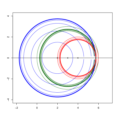
Figure 1: Gerschgorin’s discs: thin plot lines for $A$ and $A^{(t)}$ before convergence, bold plot lines for $A^{(t)}$ at convergence

Figure 1 presents the Gerschgorin discs for all iterations. The Perron root for this example is $5.739952$, the proposed algorithm and the power method require $17$ and $19$ iterations, respectively. Figure 1 shows that the major modifications of the off-diagonal elements of the matrix A are done during the first five iterations.

For all of the tests performed, the algorithm proposed and the power method have close number of iterations. Worse results, in term of the number of iterations, were obtained using a tridiagonal matrix. Let $T(n;c,a,b)$ a tridiagonal matrix of order $n$, where $a$ is the value for the diagonal components, $b$ is the value for the upper diagonal components and $c$ is the value for the under diagonal components. An explicit expression relating eigenvalues of matrix $T$ is available [23]:

$$\lambda_{k}=a+2\sqrt{bc}\cos{\frac{k\pi}{n+1}}$$ (71)

The ratio $\lambda_{2}/\lambda_{1}$ for $T$ is near $1$ when $n$ is high. For $n=50$, $a=3$, $b=2$ and $c=1$ the first two eigenvalues of matrix $T$ are: $5.823063$ and $5.806989$. The proposed algorithm took $5,890$ (algorithm A) or $5,174$ (algorithm B) iterations to calculate the Perron root. The power method need $5,159$ iterations.

Except the cases where the modulus of the second eigenvalue is near to that of the first, the algorithm proposed converges after few iterations, especially when the first eigenvalue is largely dominant. The proposed method has been succesfully used for a matrix of order $15,515$ that results from high-throughput biological data.

With a convergence rate similar to that of the classic power method, the proposed algorithm for computing the Perron root is computationally less demanding. But, it applies to only primitive matrices. However, it can be used as a low cost primitivity test compared to the matrix power calculations involved in the Frobenius and Wielandt tests.

Acknowledgements

This work was supported by funds from CNRS, INSERM and University of Strasbourg.

Author is grateful to a referee for the valuable comments and suggestions.

Appendix A R code using row sums

A.1 Algorithm B

## This function computes iteratively the Perron root
## and the eigenvector of matrix A using row sums
#
#  A: nonnegative square matrix (all row sums are > 0)
#  tol: error level used (stopping criterion)
#  maxIter: maximum number of iterations (stooping criterion)
#
# Returned
#  B: matrix which has the same row sums (B = A o X)
#  pfr: minimum and maximum row sum, that defines to the Perron root
#  y: vector (leading to have the eigenvector and matrix X)
#  iter: number of iterations performed
#  rmin: sequences with minimum row sum values for iterations
#  rmax: sequences with maximum row sum values for iterations
calcPRc <- function(A, tol=1.0e-8, maxIter=50) {
   n <- nrow(A);  m <- ncol(A)
   ri <- apply(A, 1, sum)
   ko <- (sum(A<0) || (min(ri)==0))
   if ((n != m) || (ko)) {
      stop("calcPRc(): for nonnegative primitive matrices")
   }
   y <- rep(1,n)
   iter <- 1; B <- A
   rmin <- c(); erMin <-  rmin[iter] <- min(ri)
   rmax <- c(); erMax <-  rmax[iter] <- max(ri)
   erIter <- ((erMin > tol) || (erMax > tol))
   while (erIter && (iter < maxIter)) {
         yt <- ri/ri[1]; y <- y*yt
         B <- A * ((1/y) %*% t(y))
         ri <- apply(B, 1, sum)
         iter <- iter + 1
         rmin[iter] <- ri.min <- min(ri)
         rmax[iter] <- ri.max <- max(ri)
         erMin <- rmin[iter] - rmin[iter-1]
         erMax <- rmax[iter-1] - rmax[iter]
         erIter <- ((erMin > tol) || (erMax > tol))
   }
   pfr <- c(ri.min, ri.max)
   list(B=B, pfr=pfr, y=y, iter=iter-1, rmin=rmin, rmax=rmax)
}

References

- [1] G. P. Styan, Hadamard Products and Multivariate Statistical Analysis, Linear Algebra App 6 (1973) 217–240. doi:https://doi.org/10.1016/0024-3795(73)90023-2.
- [2] R. R. Horn, C. R. Johnson, Topics in Matrix Analysis, Cambridge Univ Press, 1991.
- [3] O. Perron, Zur Theorie der Matrices, Mathematiche Annalen 64 (2) (1907) 248–263.
- [4] C. Meyer, Matrix Analysis and Applied Linear Algebra, SIAM, Philadelphia, 2000.
- [5] R. A. Brualdi, H. J. Ryser, Combinatorial matrix theory, Vol. 39 of Encyclopedia of Mathematics and its Applications, Cambridge Univ. Press, Cambridge, 1991.
- [6] A. Berman, R. J. Plemmons, Nonnegative Matrices in the Mathematical Sciences, SIAM, Philadelphia, 1994.
- [7] F. G. Frobenius, Ueber matrizen aus nicht negativen elementen, Sitzungsberichte der Königlich Preussischen Akademie der Wissenschaften” (1912) 456–477.
- [8] R. R. Horn, C. R. Johnson, Matrix Analysis, 2nd Edition, Cambridge Univ Press, 2019.
- [9] H. Wielandt, Unzerlegbare, nicht negative matrizen, Mathematische Zeitschrift 52 (1) (1950) 642–648.
- [10] G. H. Golub, C. F. V. Loan, Matrix computations, 3rd Edition, The Johns Hopkins Univ Press, Baltimore, 1996.
- [11] L. Y. Kolotilina, Lower Bounds for the Perron Root of a Nonnegative Matrix, Linear Algebra Appl 180 (1993) 133–151. doi:https://doi.org/10.1016/0024-3795(93)90528-V.
- [12] S.-L. Liu, Bounds for the Greatest Characteristic Root of a Nonnegative Matrix, Linear Algebra Appl 239 (1996) 151–160. doi:https://doi.org/10.1016/S0024-3795(96)90008-7.
- [13] X. Duan, B. Zhou, Sharp bounds on the spectral radius of a nonnegative matrix, Linear Algebra Appl 439 (2013) 2961–2970. doi:http://dx.doi.org/10.1016/j.laa.2013.08.026.
- [14] R. Xing, B. Zhou, Sharp bounds on the spectral radius of a nonnegative matrices, Linear Algebra Appl 449 (2014) 194–209. doi:http://dx.doi.org/10.1016/j.laa.2014.02.031.
- [15] P. Liao, Bounds for the Perron root of nonnegative matrices and spectral radius of iteration matrices, Linear Algebra Appl 530 (2017) 253–265. doi:http://dx.doi.org/10.1016/j.laa.2017.05.021.
- [16] L. Elsner, C. Johnson, J. Dias da Silva, The Perron Root of a Weighted Geometric Mean of Nonnegative Matrices, Linear and Multilinear Algebra 24 (1) (1988) 1–13. doi:https://doi.org/10.1080/03081088808817892.
- [17] H. Minc, Nonnegative Matrices, Wiley, New York, 1988.
- [18] R. Durbin, S. R. Eddy, A. Krogh, G. Mitchison, Biological sequences analysis, Cambridge Univ Press, Cambridge, 2002.
- [19] W. J. Ewens, G. R. Grant, Statistical methods in bioinformatics: an introduction, Springer-Verlag, New-York, 2002.
- [20] A. N. Langville, C. D. Meyer, A Survey of Eigenvector Methods for Web Information Retrival, SIAM Review 47 (1) (2005) 135–161. doi:https://doi.org/10.1137/S0036144503424786.
- [21] G. Wu, Y. Wei, A Power-Arnoldi algorithm for computing PageRank, Numer Linear Algebra Appl 14 (2007) 521–546. doi:http://dx.doi.org/10.1002/nla.531.
- [22] C. Wen, T.-Z. Huand, Z.-L. Shen, A note on the two-step matrix splitting iteration for computing PageRank, J Comput Appl Math 315 (2017) 87–97. doi:http://dx.doi.org/10.1016/j.cam.2016.10.020.
- [23] S. Noschese, L. Pasquini, L. Reichel, Tridiagonal Toeplitz matrices: properties and novel applications, Numer Linear Algebra Appl 20 (2) (2013) 302–326. doi:https://doi.org/10.1002/nla.1811.