Adaptive inference for a semiparametric generalized autoregressive conditional heteroskedasticity model

Abstract

This paper considers a semiparametric generalized autoregressive conditional heteroskedasticity (S-GARCH) model. For this model, we first estimate the time-varying long run component for unconditional variance by the kernel estimator, and then estimate the non-time-varying parameters in GARCH-type short run component by the quasi maximum likelihood estimator (QMLE). We show that the QMLE is asymptotically normal with the parametric convergence rate. Next, we construct a Lagrange multiplier test for linear parameter constraint and a portmanteau test for model checking, and obtain their asymptotic null distributions. Our entire statistical inference procedure works for the non-stationary data with two important features: first, our QMLE and two tests are adaptive to the unknown form of the long run component; second, our QMLE and two tests share the same efficiency and testing power as those in variance targeting method when the S-GARCH model is stationary.

JEL Classification: C12, C14, C58.

, and

t1Correspondence to: Department of Statistics & Actuarial Science, University of Hong Kong, Pokfulam Road, Hong Kong. E-mail address: mazhuke@hku.hk

1 Introduction

Since the seminal work of Engle (1982) and Bollerslev (1986), the generalized autoregressive conditional heteroskedasticity (GARCH) model is perhaps the most influential one to capture and forecast the volatility of economic and financial return data. However, the GARCH model is often used under the stationarity assumption. Due to business cycle, technological progress, preference change and policy switch, the underlying structure of data may change over time (see Hansen (2001)). Hence, a non-stationary GARCH model with time-varying parameters seems more appropriate to fit the return data in applications; see, for example, Mikosch and Stărică (2004), Stărică and Granger (2005), Engle and Rangel (2008), Fryzlewicz et al. (2008), Patilea and Raïssi (2014), Truquet (2017) and the references therein.

In this paper, we consider a semiparametric GARCH (S-GARCH) model of order $(p,q)$

$$y_{t}= \sqrt{\tau_{t}}u_{t}\text{ with }\tau_{t}=\tau(t/T),$$ (1.1)

$$u_{t}= \sqrt{g_{t}}\eta_{t}\text{ and }g_{t}=\omega_{0}+\sum_{i=1}^{q}\alpha_{i0}u_{t-i}^{2}+\sum_{j=1}^{p}\beta_{j0}g_{t-j},$$ (1.2)

for $t=1,...,T$, where $\tau(x)$ is a positive smoothing deterministic function with unknown form on the interval $[0,1]$, $u_{t}$ is a covariance stationary GARCH$(p,q)$ process with $\omega_{0}>0$, $\alpha_{i0}\geq 0$ and $\beta_{j0}\geq 0$, and $\{\eta_{t}\}$ is a sequence of independent and identically distributed (i.i.d) random variables with $E\eta_{t}^{2}=1$. The specification that $\tau_{t}$ is a function of ratio $t/T$ rather than time $t$ is initiated by Robinson (1989), and since then, it has become a common scaling scheme in the time series literature; see, for example, Dahlhaus and Subba Rao (2006), Cavaliere and Taylor (2007), Xu and Phillips (2008), Zhou and Wu (2009), Zhang and Wu (2012), Zhou and Shao (2013), and Zhu (2019) to name just a few. In (1.1)–(1.2), the smooth long run component $\tau_{t}$ is to depict time-varying parameters in volatility, and the GARCH-type short run component $u_{t}$ is to capture the temporal dependence.

By using different specified forms of $\tau(x)$, the S-GARCH model nests many often used models, including, for example, the standard GARCH model in Bollerslev (1986), the spline-GARCH model in Engle and Rangel (2008), and the smooth-transition GARCH model in Amado and Teräsvirta (2013). The statistical inference for these models has been well studied. However, when the specification of $\tau(x)$ is unspecified, the statistical inference for the S-GARCH model has been less attempted. For $p=q=1$, Hafner and Linton (2010) considered the estimation for the S-GARCH model. For $p=0$ (i.e., $\beta_{j0}\equiv 0$), Patilea and Raïssi (2014) constructed a score test to check the nullity of all $\alpha_{i0}$, and Truquet (2017) later proposed a projection-based estimation and a related Wald test to detect the nullity of some of $\alpha_{i0}$. For the general S-GARCH model, the statistical inference methodologies, including estimation, testing and model checking, are not available in the literature.

In this paper, we provide an entire inference procedure for the S-GARCH model to fill this gap. First, we give a two-step estimation for the model: the function $\tau(x)$ is estimated by the kernel estimator at step one, and the unknown parameter vector in the parametric process $u_{t}$ is estimated by the quasi maximum likelihood estimator (QMLE) at step two. Although the nonparametric estimator at step one has a slower convergence rate, we show that the QMLE at step two is asymptotically normal with a parametric convergence rate. Moreover, we construct a new Lagrange multiplier (LM) test for detecting the linear parameter constraint, and propose a new portmanteau test for model checking. The asymptotic null distributions of the LM and portmanteau tests are established. Since our entire inference methodologies allow for unspecified form of $\tau(x)$ and higher order $(p,q)$, they alleviate the potential risk of model-misspecification, leading to a broad application scope to handle the non-stationary data. Finally, we extend the two-step estimation to a multivariate semiparametric BEKK (S-BEKK) model, and establish the asymptotic normality of the corresponding QMLE.

Our two-step estimation was previously adopted by Hafner and Linton (2010) to study the multivariate S-BEKK(1, 1) model. For the univariate S-GARCH model, we find a much simpler expression for the asymptotic variance of the QMLE, making the related inference methodologies easy-to-implement. Meanwhile, we find that the asymptotic variance of the QMLE is adaptive to the unknown form of $\tau(x)$. Consequently, the efficiency of the QMLE and the power of its related LM and portmanteau tests are invariant regardless of the form of $\tau(x)$. However, we can show that the QMLE of the multivariate S-BEKK model no longer enjoys such an adaptiveness feature as in the univariate S-GARCH model. Our two-step estimation also shares the similar idea as the variance targeting (VT) estimation in Francq et al. (2011), which is only applicable for the stationary S-GARCH model (i.e., $\tau(x)\equiv\tau_{0}$). The difference is that our first step estimator of $\tau(x)$ is non-parametric, while the first step estimator of $\tau_{0}$ in the VT method is parametric. It turns out that our method requires more involved proof techniques. Interestingly, when the S-GARCH model is stationary, our QMLE is asymptotically as efficient as the QMLE in the second step estimation of the VT method, although the first step estimator of our method has a slower convergence rate than that of the VT method. On the contrary, when the S-GARCH is non-stationary, our QMLE is still valid with the same efficiency as the stationary case due to its adaptiveness feature, while the QMLE in the VT method is not applicable any more.

The remainder of the paper is organized as follows. Section 2 presents the two-step estimation procedure and establishes its related asymptotics. Section 3 gives a LM test for the linear parameter constraint. Section 4 introduces a portmanteau test and obtains its limiting null distribution. Section 5 makes a comparison with other estimation methods. Section 6 extends the two-step estimation into the multivariate S-BEKK model. Simulation results are reported in Section 7, and applications are given in Section 8. Concluding remarks are offered in Section 9. Proofs of all theorems are relegated to the Appendix.

2 Two-step estimation

Let $\theta=(\alpha_{1},...,\alpha_{q},\beta_{1},...,\beta_{p})^{\prime}\in\Theta$ be the parameter vector in model (1.2), and $\theta_{0}=(\alpha_{10},...,\alpha_{q0},\beta_{10},...,\beta_{p0})^{\prime}\in\Theta$ be its true value, where $\Theta\subset\mathbb{R}_{+}^{p+q}$ is the parameter space, and $\mathbb{R}_{+}=(0,\infty)$. This section gives a two-step estimation procedure for the S-GARCH model in (1.1)–(1.2). Our procedure first estimates the nonparametric function $\tau(x)$ in (1.1), and then estimates the parameter vector $\theta_{0}$ in (1.2).

2.1 Estimation of $\tau(x)$

This subsection provides a (Nadaraya-Watson) kernel estimator of $\tau(x)$. To this end, we first need an assumption for the identification of $\tau_{t}$.

Assumption 2.1.

$(\mathrm{i})$ $\sum_{i=1}^{q}\alpha_{i}+\sum_{j=1}^{p}\beta_{j}<1$; $(\mathrm{ii})$ $\omega=1-\sum_{i=1}^{q}\alpha_{i}-\sum_{j=1}^{p}\beta_{j}$.

Assumption 2.1(i) is equivalent to the covariance stationarity of model (1.2), and Assumption 2.1(ii) is to ensure $Eu_{t}^{2}=1$. Under Assumption 2.1, we have

$$y_{t}^{2}=\tau(t/T)+\tau(t/T)(u_{t}^{2}-1):=\tau(t/T)+v_{t},$$

where $v_{t}:=\tau(t/T)(u_{t}^{2}-1)$ is a zero-mean process. In other words, $y_{t}^{2}$ can be rewritten as a standard non-parametric regression problem with a time-varying mean. Following Hafner and Linton (2010), it is reasonable to estimate $\tau(x)$ by

$$\widetilde{\tau}(x)=\frac{\sum_{s=1}^{T}K_{h}\big{(}x-\frac{s}{T}\big{)}y_{s}^{2}}{\sum_{s=1}^{T}K_{h}\big{(}x-\frac{s}{T}\big{)}},$$

where $K_{h}(\cdot)=K(\cdot/h)/h$ with $K(\cdot)$ being a kernel function and $h$ being a bandwidth. Since $(1/T)\sum_{s=1}^{T}K_{h}(x-s/T)=1+O(1/(Th))$ under mild conditions, it is more convenient to estimate $\tau(x)$ by

$$\widehat{\tau}(x)=\frac{1}{T}{\sum_{s=1}^{T}K_{h}\Big{(}x-\frac{s}{T}\Big{)}y_{s}^{2}}.$$ (2.1)

To obtain the asymptotic distribution of $\widehat{\tau}(x)$, the following assumptions are needed.

Assumption 2.2.

$(\mathrm{i})$ $\tau:[0,1]\to\mathbb{R}_{+}$ is twice continuously differentiable; $(\mathrm{ii})$ $0<\underline{\tau}\leq\inf_{x\in[0,1]}\tau(x)\leq\sup_{x\in[0,1]}\tau(x)\leq\overline{\tau}$, where $\underline{\tau}$ and $\overline{\tau}$ are two positive constants.

Assumption 2.3.

$(\mathrm{i})$ $K:[-1,1]\to\mathbb{R}_{+}$ is symmetric about zero, bounded and Lipschitz continuous with $\int_{-1}^{1}K(x)dx=1$ and $C_{r}=\int_{-1}^{1}x^{r}K(x)dx$; $(\mathrm{ii})$ $h\to 0$ and $Th\to\infty$ as $T\to\infty$.

Assumption 2.4.

$Eu_{t}^{4}<\infty$.

Assumption 2.2(i) imposes a smoothness condition on $\tau(x)$, and similar conditions have been used in Dahlhaus and Subba Rao (2006), Hafner and Linton (2010), and Chen and Hong (2016). Assumption 2.2(ii) is in line with the condition that the intercept term in the standard GARCH model has positive lower and upper bounds. Assumption 2.3(i) holds for many often used kernels, and the bounded support condition on $K(x)$ is just to simplify analysis. Assumption 2.3(ii) requires that $h$ converges to zero at a slower rate than $T^{-1}$, and later a more restrictive $h$ is needed for the asymptotics of the estimator of $\theta_{0}$. Assumption 2.4 is stronger than Assumption 2.1(i), and it is used to ensure that the asymptotic variance of $\widehat{\tau}(x)$ is well defined.

Let $z_{t}=u_{t}^{2}-1$. The asymptotic normality of $\widehat{\tau}(x)$ is given below.

Theorem 2.1.

Suppose Assumptions 2.1–2.4 hold. Then, for any $x\in(0,1)$,

$$\sqrt{Th}\big{(}\widehat{\tau}(x)-\tau(x)-h^{2}b(x)\big{)}\to_{\mathcal{L}}N(0,V(x))\mbox{ as }T\to\infty,$$

where ‘$\to_{\mathcal{L}}$’ stands for the convergence in distribution,

$$b(x)=\frac{C_{2}}{2}\frac{\partial^{2}\tau(x)}{\partial x^{2}}\mbox{ and }V(x)=\tau^{2}(x)\Big{\{}\int_{-1}^{1}K^{2}(x)dx\Big{\}}\sum_{j=-\infty}^{\infty}E(z_{t}z_{t-j}).$$

Based on $\widehat{\tau}(x)$ in (2.1), we estimate $\tau_{t}$ by $\widehat{\tau}_{t}=\widehat{\tau}(t/T)$. In practice, $\widehat{\tau}_{t}$ may have the boundary problem. To circumvent this problem, we follow Chen and Hong (2016) to adopt the reflection method proposed by Hall and Wehrly (1991). That is, we generate pseudo data $y_{t}=y_{-t}$ for $-[Th]\leq t\leq-1$ and $y_{t}=y_{2T-t}$ for $T+1\leq t\leq T+[Th]$, and then modify $\widehat{\tau}_{t}$ as

$$\widehat{\tau}_{t}=\frac{1}{T}\sum_{s=t-[Th]}^{t+[Th]}K_{h}\Big{(}\frac{t-s}{T}\Big{)}y_{s}^{2}.$$ (2.2)

Intuitively, the reflection method makes the boundary points behave similarly as the interior ones. Similar to Chen and Hong (2016), it can be seen that the reflection method gives a bias term of order $O(h^{2})$, and hence it does not affect the asymptotics of the estimator of $\theta_{0}$. Although $\widehat{\tau}_{t}$ in (2.2) is used for numerical calculations, our proofs below will be based on $\widehat{\tau}_{t}=\widehat{\tau}(t/T)$ in (2.1) to ease the presentation.

2.2 Estimation of $\theta_{0}$

This subsection considers the QMLE of $\theta_{0}$. Based on Assumption 2.1(ii), we write the parametric $g_{t}$ in (1.2) as

$$g_{t}(\theta)=\Big{(}1-\sum_{i=1}^{q}\alpha_{i}-\sum_{j=1}^{p}\beta_{j}\Big{)}+\sum_{i=1}^{q}\alpha_{i}u_{t-i}^{2}+\sum_{j=1}^{p}\beta_{j}g_{t-j}(\theta).$$ (2.3)

By assuming that $\eta_{t}\sim N(0,1)$, the log-likelihood function (multiplied by -2 and ignoring constants) of $\{y_{t}\}$ is

$$L_{T}(\theta)=\sum_{t=1}^{T}l_{t}(\theta)\quad\text{with}\quad l_{t}(\theta)=\frac{u_{t}^{2}}{g_{t}(\theta)}+\log g_{t}(\theta).$$ (2.4)

Unfortunately, $L_{T}(\theta)$ is infeasible for computation, since $\{u_{t}\}$ are unobservable. Thus, we have to replace $\{u_{t}\}$ by $\{\widehat{u}_{t}\}$, and consider the following feasible log-likelihood function

$$\widehat{L}_{T}(\theta)=\sum_{t=1}^{T}\widehat{l}_{t}(\theta)\quad\text{with}\quad\widehat{l}_{t}(\theta)=\frac{\widehat{u}_{t}^{2}}{\widehat{g}_{t}(\theta)}+\log\widehat{g}_{t}(\theta),$$ (2.5)

where $\widehat{u}_{t}=y_{t}/\sqrt{\widehat{\tau}_{t}}$, and $\widehat{g}_{t}(\theta)$ is computed recursively by

$$\widehat{g}_{t}(\theta)=\Big{(}1-\sum_{i=1}^{q}\alpha_{i}-\sum_{j=1}^{p}\beta_{j}\Big{)}+\sum_{i=1}^{q}\alpha_{i}\widehat{u}_{t-i}^{2}+\sum_{j=1}^{p}\beta_{j}\widehat{g}_{t-j}(\theta)$$ (2.6)

with given constant initial values

$$\widehat{u}_{0}=u_{0},...,\,\widehat{u}_{1-q}=u_{q-1},\,\widehat{g}_{0}(\theta)=g_{0},...,\,\widehat{g}_{1-p}(\theta)=g_{1-p}.$$

Based on $\widehat{L}_{T}(\theta)$ in (2.5), our QMLE of $\theta_{0}$ is defined as

$$\widehat{\theta}_{T}=\arg\min_{\theta\in\Theta}\widehat{L}_{T}(\theta).$$

To establish the asymptotics of $\widehat{\theta}_{T}$, denote $\mathcal{A}_{\theta}(z)=\sum_{i=1}^{q}\alpha_{i}z^{i}$ and $\mathcal{B}_{\theta}(z)=1-\sum_{i=1}^{p}\beta_{i}z^{i}$ with the convention $\mathcal{A}_{\theta}(z)=0$ if $q=0$ and $\mathcal{B}_{\theta}(z)=1$ if $p=0$. The following additional assumptions are imposed.

Assumption 2.5.

$(\mathrm{i})$ $\Theta$ is compact; $(\mathrm{ii})$ if $p>0$, the polynomials $\mathcal{A}_{\theta_{0}}(z)$ and $\mathcal{B}_{\theta_{0}}(z)$ have no common roots, $\mathcal{A}_{\theta_{0}}(1)\neq 0$, and $\alpha_{q0}+\beta_{p0}\neq 0$; $(\mathrm{iii})$ $\theta_{0}$ is an interior point of $\Theta$.

Assumption 2.6.

$E|u_{t}|^{4(1+\delta_{0})}<\infty$ for some $\delta_{0}>0$.

Assumption 2.7.

$(\mathrm{i})$ $\eta_{t}$ has a continuous and almost surely positive density on $\mathbb{R}$ with $E\eta_{t}^{2}=1$; $(\mathrm{ii})$ $E|\eta_{t}|^{4+4/\delta_{0}+\delta_{1}}<\infty$ for some $\delta_{1}>0$, where $\delta_{0}>0$ is defined as in Assumption 2.6.

Assumption 2.8.

$h=c_{h}T^{-\lambda_{h}}$ for some $1/4<\lambda_{h}<1/2$ and $0<c_{h}<\infty$.

We offer some remarks on the aforementioned assumptions. Assumption 2.5 is regular, and it has been used in Horváth and Kokoszka (2003) and Francq and Zakoïan (2004) to study the QMLE for the stationary GARCH model. Assumption 2.6 is stronger than Assumption 2.4, which is needed for the variance target estimator in Francq et al. (2011) but not for the QMLE in Francq and Zakoïan (2004). Assumption 2.7(i) gives the identification condition for $\theta_{0}$ based on the QMLE, and ensures that the GARCH process $u_{t}$ is $\beta$-mixing (see Carrasco and Chen (2002)). Assumption 2.7(ii) is stronger than the condition $E\eta_{t}^{4}<\infty$, which is necessary to derive the asymptotic normality of the QMLE for the stationary GARCH model (see Hall and Yao (2003)). We resort to the stronger conditions of $u_{t}$ and $\eta_{t}$ in Assumptions 2.6 and 2.7(ii) due to the existence of $\tau(x)$ in the S-GARCH model. Note that if $\eta_{t}$ has a light tail (for example, $\eta_{t}\sim N(0,1)$), Assumption 2.7(ii) holds for a small value of $\delta_{0}$, and $u_{t}$ (or the data $y_{t}$) in Assumption 2.6 is thus allowed to be heavy-tailed. Assumption 2.8 requires a more restrictive condition on the bandwidth $h$ than Assumption 2.3(ii), and similar conditions have been adopted by Hafner and Linton (2010), Patilea and Raïssi (2014), and Truquet (2017). The reason is because an undersmoothing $h$ is needed to make the estimation bias from $\widehat{\tau}_{t}$ negligible so that the $\sqrt{T}$-convergence of $\widehat{\theta}_{T}$ holds.

Denote $\kappa=E\eta_{t}^{4}$, $g_{t}=g_{t}(\theta_{0})$, $\psi_{t}=\psi_{t}(\theta_{0})$ with $\psi_{t}(\theta)=\{\partial g_{t}(\theta)/\partial\theta\}/g_{t}(\theta)$, and

$$J_{1} =E(\psi_{t}\psi_{t}^{\prime}),\,\,\,J_{2}=E(g_{t}^{2})E\big{(}\psi_{t}/g_{t}\big{)}E\big{(}\psi_{t}^{\prime}/g_{t}\big{)}.$$ (2.7)

Now, we are ready to give the asymptotics of $\widehat{\theta}_{T}$ in the following theorem.

Theorem 2.2.

Suppose Assumptions 2.1–2.3, 2.5(i)–(ii), and 2.6–2.7 hold. Then,

$\mathrm{(i)}$ $\widehat{\theta}_{T}\to_{p}\theta_{0}$ as $T\to\infty$;

$\mathrm{(ii)}$ furthermore, if Assumption 2.5(iii) holds and Assumption 2.3(ii) is replaced by Assumption 2.8,

$$\sqrt{T}(\widehat{\theta}_{T}-\theta_{0})\to_{\mathcal{L}}N(0,\Sigma)\mbox{ as }T\to\infty,$$

where $\Sigma=(\kappa-1)J_{1}^{-1}(J_{1}+J_{2})J_{1}^{-1}$, and $J_{1}$ and $J_{2}$ are defined in (2.7).

Remark 1.

We can simply estimate $\Sigma$ by its sample version $\widehat{\Sigma}_{T}$, where

$$\widehat{\Sigma}_{T}=(\widehat{\kappa}_{T}-1)\widehat{J}_{1T}^{-1}(\widehat{J}_{1T}+\widehat{J}_{2T})\widehat{J}_{1T}^{-1}$$ (2.8)

with

$$\begin{split}\widehat{\kappa}_{T}=\frac{1}{T}\sum_{t=1}^{T}\widehat{\eta}_{t}^{4},\,\,\widehat{J}_{1T}=\frac{1}{T}\sum_{t=1}^{T}\widehat{\psi}_{t}\widehat{\psi}_{t}^{\prime}\mbox{ and }\,\,\widehat{J}_{2T}=\Big{(}\frac{1}{T}\sum_{t=1}^{T}\widehat{g}_{t}^{2}\Big{)}\Big{(}\frac{1}{T}\sum_{t=1}^{T}\frac{\widehat{\psi}_{t}}{\widehat{g}_{t}}\Big{)}\Big{(}\frac{1}{T}\sum_{t=1}^{T}\frac{\widehat{\psi}_{t}^{\prime}}{\widehat{g}_{t}}\Big{)}.\end{split}$$ (2.9)

Here, $\widehat{\eta}_{t}=\widehat{\eta}_{t}(\widehat{\theta}_{T})$ with $\widehat{\eta}_{t}(\theta)=\widehat{u}_{t}/\sqrt{\widehat{g}_{t}(\theta)}$, $\widehat{\psi}_{t}=\widehat{\psi}_{t}(\widehat{\theta}_{T})$ with $\widehat{\psi}_{t}(\theta)=\{\partial\widehat{g}_{t}(\theta)/\partial\theta\}/\widehat{g}_{t}(\theta)$, and $\widehat{g}_{t}=\widehat{g}_{t}(\widehat{\theta}_{T})$. Under the conditions of Theorem 2.2, we have $\widehat{\Sigma}_{T}\to_{p}\Sigma$ as $T\to\infty$.

Interestingly, the preceding theorem shows that the asymptotic variance of $\widehat{\theta}_{T}$ is independent of $\tau(x)$. Following the viewpoint of Robinson (1987), it means that $\widehat{\theta}_{T}$ is adaptive to the unknown form of $\tau(x)$. This adaptiveness feature ensures that the efficiency of $\widehat{\theta}_{T}$ and the power of its related tests are unchanged regardless of the form of $\tau(x)$.

3 The LM test

Since Engle (1982) and Bollerslev (1986), testing for the nullity of the parameters in the GARCH model is important in applications. This problem can be further generalized to consider the following linear constraint hypothesis

$$\mathbb{H}_{0}:R\theta_{0}=r,$$ (3.1)

where $R$ is a given $d\times(p+q)$ matrix of rank $d$, and $r$ is a given $d\times 1$ constant vector. In this section, we construct a Lagrange multiplier (LM) test statistic $LM_{T}$ for $\mathbb{H}_{0}$, where

$$LM_{T}=\frac{1}{T}\frac{\partial\widehat{L}_{T}(\widehat{\theta}_{T|0})}{\partial\theta^{\prime}}\widehat{J}_{1T|0}^{-1}R^{\prime}\big{(}R\widehat{\Sigma}_{T|0}R^{\prime}\big{)}^{-1}R\widehat{J}_{1T|0}^{-1}\frac{\partial\widehat{L}_{T}(\widehat{\theta}_{T|0})}{\partial\theta}.$$

Here, $\widehat{\theta}_{T|0}$ is the constrained QMLE of $\theta_{0}$ under $\mathbb{H}_{0}$, and $\widehat{J}_{1T|0}$ and $\widehat{\Sigma}_{T|0}$ are defined in the same way as $\widehat{J}_{1T}$ and $\widehat{\Sigma}_{T}$, respectively, with $\widehat{\theta}_{T}$ replaced by $\widehat{\theta}_{T|0}$. The following theorem gives the limiting null distribution of $LM_{T}$.

Theorem 3.1.

Suppose the conditions in Theorem 2.2(i) hold, with Assumption 2.3(ii) replaced by Assumption 2.8. Then, under $\mathbb{H}_{0}$,

$$LM_{T}\to_{\mathcal{L}}\chi^{2}_{d}\mbox{ as }T\to\infty,$$

where $\chi^{2}_{d}$ is the chi-square distribution with the degrees of freedom $d$.

Based on Theorem 3.1, we can set the rejection region of $LM_{T}$ at level $\alpha$ as $\{LM_{T}>\chi_{d}^{2}(\alpha)\},$ where $\chi_{d}^{2}(\alpha)$ is the $\alpha$-upper percentile of $\chi_{d}^{2}$.

As $\widehat{\theta}_{T}$, our $LM_{T}$ has the adaptiveness feature, and it has a much broader application scope than the existing LM tests. Specifically, the LM test in Bollerslev (1986) is only applicable for the stationary GARCH model, but our $LM_{T}$ has the superior ability to tackle the non-stationary S-GARCH model. For the case of $p=0$, the score test in Patilea and Raïssi (2014) can detect the null hypothesis that all $\alpha_{i0}$ are zeros, and the Wald test in Truquet (2017) can check the null hypothesis that some of $\alpha_{i0}$ are zeros. However, it seems non-trivial to extend these two tests for the general null hypotheses in (3.1), although the score test in Patilea and Raïssi (2014) can be extended to detect the null hypothesis that all $\alpha_{i0}$ and $\beta_{j0}$ are zeros. Besides $LM_{T}$, the Wald and likelihood ratio (LR) tests could also be constructed for $\mathbb{H}_{0}$. When some of $\alpha_{i0}$ or $\beta_{j0}$ are allowed to be zeros under $\mathbb{H}_{0}$, the Wald and LR tests render non-standard limiting null distributions (see Francq and Zakoïan (2009) for general discussions), which have to be simulated by the bootstrap method. In contrast, $LM_{T}$ always has the standard chi-square limiting null distribution, even when all of the null coefficients are not pinned down in $\mathbb{H}_{0}$. For practical convenience, we thus only focus on the LM test in this paper, and the consideration of Wald and LR tests is left for future study.

4 Portmanteau test

Since Ljung and Box (1978), the portmanteau test and its variants have been a common tool for checking the model adequacy in time series analysis. For the stationary GARCH model, Li and Mak (1994) proposed a portmanteau test for model checking. However, their test is invalid for the non-stationary S-GARCH model. In this section, we follow the idea of Li and Mak (1994) to construct a new portmanteau test to check the adequacy of S-GARCH model, and our test seems to be the first formal try in the context of semiparametric time series analysis.

Let $\widehat{\eta}_{t}$ be the model residual defined as in (2.9). The idea of our portmanteau test is based on the fact that $\{\eta_{t}^{2}\}$ is a sequence of uncorrelated random variables under (1.1)–(1.2). Hence, if the S-GARCH model is correctly specified, it is expected that the sample autocorrelation function of $\{\widehat{\eta}_{t}^{2}\}$ at lag $k$, denoted by $\widehat{\rho}_{T,k}$, is close to zero, where

$$\widehat{\rho}_{T,k}=\frac{\sum_{t=k+1}^{T}\big{(}\widehat{\eta}^{2}_{t}-\overline{\widehat{\eta}^{2}}\big{)}\big{(}\widehat{\eta}^{2}_{t-k}-\overline{\widehat{\eta}^{2}}\big{)}}{\sum_{t=1}^{T}\big{(}\widehat{\eta}^{2}_{t}-\overline{\widehat{\eta}^{2}}\big{)}^{2}}$$

with $\overline{\widehat{\eta}^{2}}$ being the sample mean of $\{\widehat{\eta}_{t}^{2}\}$. Let $\widehat{\rho}_{T}=(\widehat{\rho}_{T,1},...,\widehat{\rho}_{T,\ell})^{\prime}$ for an integer $\ell\geq 1$, and

$$\Sigma_{P1} =(I_{\ell},-H,-DJ_{1}^{-1})\in\mathbb{R}^{\ell\times(\ell+1+p+q)},$$ (4.1)

$$\Sigma_{P2} =\left(\begin{matrix}(\kappa-1)I_{\ell}&F&D-FE\big{(}\frac{\psi_{t}^{\prime}}{g_{t}}\big{)}\\ *&Eg_{t}^{2}&-Eg_{t}^{2}E\big{(}\frac{\psi_{t}^{\prime}}{g_{t}}\big{)}\\ *&*&J_{1}+J_{2}\end{matrix}\right)\in\mathbb{R}^{(\ell+1+p+q)\times(\ell+1+p+q)}$$ (4.2)

be a symmetric matrix, where $D=(D_{1}^{\prime},...,D_{\ell}^{\prime})^{\prime}$ with $D_{k}=E\{(\eta_{t-k}^{2}-1)\psi_{t}^{\prime}\}$, $H=(H_{1},...,H_{\ell})^{\prime}$ with $H_{k}=E\{g_{t}^{-1}(\eta_{t-k}^{2}-1)\}$, and $F=(F_{1},...,F_{\ell})^{\prime}$ with $F_{k}=E\{g_{t}(\eta_{t-k}^{2}-1)\}$. To facilitate our portmanteau test, we need the limiting distribution of $\widehat{\rho}_{T}$ below.

Theorem 4.1.

Suppose the conditions in Theorem 2.2(ii) hold. Then, if the S-GARCH model in (1.1)–(1.2) is correctly specified,

$$\sqrt{T}\widehat{\rho}_{T}\to_{\mathcal{L}}N(0,\Sigma_{P})\mbox{ as }T\to\infty,$$

where $\Sigma_{P}=(\kappa-1)^{-1}\Sigma_{P1}\Sigma_{P2}\Sigma_{P1}^{\prime}$, and $\Sigma_{P1}$ and $\Sigma_{P2}$ are defined in (4.1)–(4.2).

As in Remark 1, $\Sigma_{P}$ can be consistently estimated by its sample version $\widehat{\Sigma}_{P}$. Based on $\widehat{\Sigma}_{P}$, our portmanteau test statistic is defined as

$$Q_{T}(\ell)=T\widehat{\rho}_{T}^{\prime}\widehat{\Sigma}_{P}^{-1}\widehat{\rho}_{T}.$$

If the S-GARCH model is correctly specified, $Q_{T}(\ell)\to_{\mathcal{L}}\chi^{2}_{\ell}$ as $T\to\infty$ by Theorem 4.1. So, if the value of $Q_{T}(\ell)$ is larger than $\chi_{\ell}^{2}(\alpha)$, the fitted S-GARCH model is inadequate at level $\alpha$. Otherwise, it is adequate at level $\alpha$. In practice, the choice of lag $\ell$ depends on the frequency of the series, and one often chooses $\ell$ to be $O(\log(T))$, delivering 6, 9 or 12 for a moderate $T$. We shall hightlight that $Q_{T}(\ell)$ also has the adaptiveness feature as $LM_{T}$, and it is essential to detect the adequacy of the short run GARCH component $u_{t}$ but not the long run component $\tau_{t}$, since the form of $\tau_{t}$ is unspecified in the S-GARCH model.

5 Comparisons with other estimation methods

This section compares our two-step estimation method with the three-step estimation method in Hafner and Linton (2010) and the variance targeting (VT) estimation method in Francq et al. (2011).

5.1 Comparison with three-step estimation method

Our two-step estimation method is the same as the first two estimation steps in Hafner and Linton (2010), where they gave the following asymptotic normality result for the S-GARCH($1,1$) model

$$\sqrt{T}(\widehat{\theta}_{T}-\theta_{0})\to_{\mathcal{L}}N(0,\Sigma_{{\dagger}})\mbox{ as }T\to\infty,$$

where $\Sigma_{{\dagger}}=J_{1}^{-1}[(\kappa-1)J_{1}+J_{3}+J_{4}+J_{4}^{\prime}]J_{1}^{-1}$ with $J_{3}=(M-E\psi_{t})(M-E\psi_{t})^{\prime}Z_{1}$, $J_{4}=Z_{2}(M-E\psi_{t})^{\prime}$,

$$M=\sum_{j=0}^{\infty}\alpha_{10}\beta_{10}^{j}E\Big{(}\frac{u^{2}_{t-j-1}\psi_{t}}{g_{t}}\Big{)},\,\,Z_{1}=\sum_{j=-\infty}^{\infty}E(z_{t}z_{t-j})\,\,\mbox{ and }\,\,Z_{2}=\sum_{j=0}^{\infty}E\big{\{}z_{t}(\eta_{t-j}^{2}-1)\psi_{t-j}\big{\}}.$$

Indeed, we can show that $\Sigma_{{\dagger}}$ and $\Sigma$ are equivalent. Since $\Sigma_{{\dagger}}$ involves three infinite summations $M$, $Z_{1}$ and $Z_{2}$, a consistent estimator for $\Sigma_{{\dagger}}$ then involves laborious tuning and smoothing. On the contrary, our $\Sigma$ has a much simpler expression, and it can be directly estimated as shown in Remark 1.

In Hafner and Linton (2010), they further proposed an updated estimator at step three, and claimed this updated estimator can achieve the semiparametric efficiency bound when $\eta_{t}\sim N(0,1)$. Following their idea, we can also update our estimator $\widehat{\theta}_{T}$ to $\widecheck{\theta}_{T}$ at step three. Specifically, we first update the nonparametric part estimator $\widehat{\tau}_{t}$ to $\widecheck{\tau}_{t}=\widecheck{\tau}(t/T)$, where

$$\widecheck{\tau}(x)=\widehat{\tau}(x)-\Big{[}\frac{1}{T}\sum_{t=1}^{T}K_{h}\Big{(}x-\frac{t}{T}\Big{)}\frac{\partial^{2}\widehat{l}_{t}(\widehat{\tau},\widehat{\theta}_{T})}{\partial\tau^{2}}\Big{]}^{-1}\Big{[}\frac{1}{T}\sum_{t=1}^{T}K_{h}\Big{(}x-\frac{t}{T}\Big{)}\frac{\partial\widehat{l}_{t}(\widehat{\tau},\widehat{\theta}_{T})}{\partial\tau}\Big{]}$$

with

$$\widehat{l}_{t}({\tau},\widehat{\theta}_{T})=\log\widehat{g}_{t}(\widehat{\theta}_{T})+\log(\tau)+\frac{y_{t}^{2}}{{\tau}\widehat{g}_{t}(\widehat{\theta}_{T})}.$$

Then, based on $\widecheck{u}_{t}^{2}=y_{t}^{2}/\widecheck{\tau}_{t}$ and some given initial values, we calculate

$$\widecheck{g}_{t}(\theta)=1-\sum_{i=1}^{q}\alpha_{i}-\sum_{j=1}^{p}\beta_{j}+\sum_{i=1}^{q}\alpha_{i}\widecheck{u}_{t-i}^{2}+\sum_{j=1}^{p}\beta_{j}\widecheck{g}_{t-j}(\theta),$$

and update the parametric part estimator $\widehat{\theta}_{T}$ to $\widecheck{\theta}_{T}$ as follows:

$$\widecheck{\theta}_{T}=\widehat{\theta}_{T}-\Big{[}\frac{\partial^{2}\widecheck{L}_{T}^{*}(\widehat{\theta}_{T})}{\partial\theta\partial\theta^{\prime}}\Big{]}^{-1}\frac{\partial\widecheck{L}_{T}^{*}(\widehat{\theta}_{T})}{\partial\theta},$$

where

$$\frac{\partial\widecheck{L}_{T}^{*}(\widehat{\theta}_{T})}{\partial\theta}= \sum_{t=1}^{T}\Big{[}\widecheck{g}_{t}(\widehat{\theta}_{T})^{-1}\frac{\partial\widecheck{g}_{t}(\widehat{\theta}_{T})}{\partial\theta}-\widecheck{G}_{T}(\widehat{\theta}_{T})\Big{]}(1-\widecheck{\eta}_{t}(\widehat{\theta}_{T})^{2}),$$

$$\frac{\partial^{2}\widecheck{L}_{T}^{*}(\widehat{\theta}_{T})}{\partial\theta\partial\theta^{\prime}}= \sum_{t=1}^{T}\Big{[}\widecheck{g}_{t}(\widehat{\theta}_{T})^{-2}\frac{\partial\widecheck{g}_{t}(\widehat{\theta}_{T})}{\partial\theta}\frac{\partial\widecheck{g}_{t}(\widehat{\theta}_{T})}{\partial\theta^{\prime}}-\widecheck{G}_{T}(\widehat{\theta}_{T})\widecheck{G}(\widehat{\theta}_{T})^{\prime}\Big{]}$$

with $\widecheck{G}_{T}(\theta)=\frac{1}{T}\sum_{t=1}^{T}\widecheck{g}_{t}(\theta)^{-1}\frac{\partial\widecheck{g}_{t}(\theta)}{\partial\theta}$. Below, we give the limiting distribution of $\widecheck{\theta}_{T}$.

Theorem 5.1.

Suppose the conditions in Theorem 2.2(ii) hold. Then,

$$\sqrt{T}(\widecheck{\theta}_{T}-\theta_{0})\to_{\mathcal{L}}N(0,\Sigma^{*})\mbox{ as }T\to\infty,$$

where $\Sigma^{*}=(\kappa-1)J_{1}^{*-1}(J_{1}^{*}+J_{2}^{*})J_{1}^{*-1}$ with

$$J_{1}^{*}= E\{(\psi_{t}-E\psi_{t})(\psi_{t}-E\psi_{t})^{\prime}\},$$

$$J_{2}^{*}= \frac{\omega_{0}^{2}}{\gamma_{0}^{2}}\Big{[}Eg_{t}^{-1}E\psi_{t}-Eg_{t}^{-1}\psi_{t}\Big{]}\Big{[}Eg_{t}^{-1}E\psi_{t}-Eg_{t}^{-1}\psi_{t}\Big{]}^{\prime},$$

and $\omega_{0}=1-\sum_{i=1}^{q}\alpha_{i0}-\sum_{j=1}^{p}\beta_{j0}$ and $\gamma_{0}=1-\sum_{j=1}^{p}\beta_{j0}$.

The preceding theorem shows that $\widecheck{\theta}_{T}$ can not achieve the semiparametric efficiency bound as $J_{2}^{*}$ is positive definite. Hence, it seems unnecessary to consider the third estimation step in Hafner and Linton (2010). Note that the above updating procedure was also given by Bickel et al. (1993), in which they showed the updated estimator can achieve the semiparametric efficiency bound when the data are independent. However, when the data are dependent, their conclusion may not be true as demonstrated by Theorem 5.1. The failure of $\widecheck{\theta}_{T}$ in our case possibly results from the violation of the following condition

$$\frac{1}{\sqrt{T}}\Big{\{}\frac{\partial\widecheck{L}_{T}^{*}(\widehat{\theta}_{T})}{\partial\theta}-\frac{\partial{L}_{T}^{*}(\widehat{\theta}_{T})}{\partial\theta}\Big{\}}=o_{p}(1),$$ (5.1)

where $\frac{\partial L_{T}^{*}(\theta)}{\partial\theta}$ is defined in the same way as $\frac{\partial\widecheck{L}_{T}^{*}(\theta)}{\partial\theta}$ with $\widecheck{u}_{t}$ and $\widecheck{g}_{t}({\theta})$ replaced by $u_{t}$ and ${g}_{t}({\theta})$, respectively. In Bickel et al. (1993), a condition similar to (5.1) was proved for the independent data. However, their technical treatment does not work in our time series setting. This is because in the updating procedure at step three, the process $\widecheck{g}_{t}$ utilizes the information before and after time period $t$, so that they are not independent of $\{u_{s}^{2}\}_{s\neq t}$.

5.2 Comparison with VT estimation method

Our two-step estimation method also has a linkage to the VT estimation method in Francq et al. (2011), and this aspect has not been explored before. The VT method is designed for the following covariance stationary GARCH($p,q$) model

$$\begin{split}&y_{t}=\sqrt{h_{t}}\eta_{t}\\ &\text{with }h_{t}=\tau_{0}\Big{(}1-\sum_{i=1}^{q}\alpha_{i0}-\sum_{j=1}^{p}\beta_{j0}\Big{)}+\sum_{i=1}^{q}\alpha_{i0}y_{t-i}^{2}+\sum_{j=1}^{p}\beta_{j0}h_{t-j},\end{split}$$ (5.2)

where $\tau_{0}$ is a positive parameter, and $\alpha_{i0}$, $\beta_{j0}$ and $\eta_{t}$ are defined as before. Indeed, model (5.2) is just our stationary S-GARCH model, and it is also an alternative reparametrization version of the conventional covariance stationary GARCH model. Since $Ey_{t}^{2}=\tau_{0}$ under model (5.2), the VT method first estimates $\tau_{0}$ by $\overline{\tau}_{T}$, and then estimates $\theta_{0}$ by the QMLE $\overline{\theta}_{T}$, where

$$\begin{split}\overline{\tau}_{T}=\frac{1}{T}\sum_{t=1}^{T}y_{t}^{2}\mbox{ and }\overline{\theta}_{T}=\arg\min_{\theta\in\Theta}\overline{L}_{T}(\theta)\mbox{ with }\overline{L}_{T}(\theta)=\sum_{t=1}^{T}\frac{\overline{u}_{t}^{2}}{\overline{g}_{t}(\theta)}+\log\overline{g}_{t}(\theta).\end{split}$$ (5.3)

Here, $\overline{u}_{t}=y_{t}/\sqrt{\overline{\tau}_{T}}$, and $\overline{g}_{t}(\theta)$ is defined in the same way as $\widehat{g}_{t}(\theta)$ in (2.6) with $\widehat{u}_{t}$ replaced by $\overline{u}_{t}$. Clearly, the difference of two methods is that our method estimates the unknown function $\tau(x)$ nonparametrically, while the VT method estimates the unknown constant parameter $\tau_{0}$ by the sample mean of $y_{t}^{2}$. It turns out that two methods require different technical treatments and give different application scopes. From a statistical point of view, the proof techniques for VT method rely on the facts that the objective function $\overline{L}_{T}(\theta)$ is differential around $\tau_{0}$ and the first step estimator $\overline{\tau}_{T}$ is $\sqrt{T}$-consistent. However, neither of these facts holds for our method, and we thus need develop new proof techniques based on more restrictive conditions for $u_{t}$ and $\eta_{t}$. From a practical point of view, our method works for the either stationary or non-stationary S-GARCH model, while the VT method does only for the stationary S-GARCH model. Hence, our method has a much broader application scope than the VT method.

By revisiting Theorem 2.1 in Francq et al. (2011), we further find that the asymptotic variance of $\overline{\theta}_{T}$ is the same as the one of $\widehat{\theta}_{T}$ in Theorem 2.2. That is, our QMLE $\widehat{\theta}_{T}$ and the QMLE $\overline{\theta}_{T}$ in the VT method have the same asymptotic efficiency, although our first step estimator has a slower convergence rate $\sqrt{Th}$ than the parametric convergence rate $\sqrt{T}$. This novel feature has not been discovered in the literature, and it makes our two-step method more attractive than the VT method, since our QMLE does not suffer any efficiency loss for the stationary S-GARCH model, and at the same time, our QMLE can still work with the same efficiency (due to the adaptiveness feature) for the non-stationary S-GARCH model. As expected, similar features also hold for our tests $LM_{T}$ and $Q_{T}(\ell)$, and these findings will be further illustrated by simulation studies.

6 Extension to multivariate S-BEKK model

In this section, we extend the two-step estimation for the S-GARCH model to the multivariate semiparametric BEKK (S-BEKK) model. Let $\{\mathbf{y}_{t}\}_{t=1}^{T}$ be a sequence of random vectors with dimension $N\geq 1$. Assume $\mathbf{y}_{t}$ satisfies the following S-BEKK model

$$\mathbf{y}_{t}= \mathbb{\boldsymbol{\tau}}_{t}^{1/2}\mathbf{u}_{t}~{}\mbox{with}~{}\mathbb{\boldsymbol{\tau}}_{t}=\mathbb{\boldsymbol{\tau}}(t/T),$$ (6.1)

$$\mathbf{u}_{t}= \mathbf{g}_{t}^{1/2}\boldsymbol{\eta}_{t}~{}\mbox{and}~{}\mathbf{g}_{t}=W_{0}+\sum_{i=1}^{q}A_{i0}\mathbf{u}_{t-i}\mathbf{u}_{t-i}^{\prime}A_{i0}^{\prime}+\sum_{j=1}^{p}B_{j0}\mathbf{g}_{t-j}B_{j0}^{\prime},$$ (6.2)

for $t=1,...,T$, where $\mathbb{\boldsymbol{\tau}}(x)\in\mathbb{R}^{N\times N}$ is a positively definite, smoothing and deterministic matrix with unknown form on the interval $[0,1]$, $\mathbf{u}_{t}$ is a covariance stationary BEKK$(p,q)$ process parameterized by $N\times N$ matrices $A_{i0}$, $i=1,...,q$, $B_{j0}$, $j=1,...,p$ and $W_{0}:=I_{N}-\sum_{i=1}^{q}A_{i0}A_{i0}^{\prime}-\sum_{j=1}^{p}B_{j0}B_{j0}^{\prime}$, and $\{\boldsymbol{\eta}_{t}\}$ is a sequence of i.i.d random vectors satisfying $E\boldsymbol{\eta}_{t}\boldsymbol{\eta}_{t}^{\prime}=I_{N}$. Clearly, our S-BEKK model reduces to the standard BEKK model in Engle and Kroner (1995) when $\mathbb{\boldsymbol{\tau}}(x)$ is a constant matrix, and it includes the first-order S-BEKK model in Hafner and Linton (2010) as a special case.

Let $\mathrm{tr}(A)$ and $\mathrm{det}(A)$ be the trace and determinant of a matrix $A$, respectively, $\mathrm{vec}(A)$ be the vectorization of a matrix $A$ by stacking its columns, $A\otimes B$ be the Kronecker product between two matrices $A$ and $B$, and $A^{\otimes 2}=A\otimes A$. Denote $\boldsymbol{\theta}=(\mathrm{vec}(A_{1})^{\prime},...,\mathrm{vec}(A_{q})^{\prime},\mathrm{vec}(B_{1})^{\prime},$ $...,\mathrm{vec}(B_{p})^{\prime})^{\prime}\in\boldsymbol{\Theta}$ be the unknown parameter of $\mathbf{u}_{t}$, and $\boldsymbol{\Theta}\subset\mathbb{R}^{\mathrm{dim}(\mathbb{\boldsymbol{\theta}})}$ be the parameter space, where $\mathrm{dim}(\mathbb{\boldsymbol{\theta}})$ stands for the dimension of $\boldsymbol{\theta}$. Similar to the S-GARCH model, we consider the two-step estimation for the S-BEKK model. At step one, we estimate $\mathbb{\boldsymbol{\tau}}_{t}$ by $\widehat{\mathbb{\boldsymbol{\tau}}}_{t}=\widehat{\mathbb{\boldsymbol{\tau}}}(t/T)$, where

$$\widehat{\mathbb{\boldsymbol{\tau}}}(x)=\frac{1}{T}{\sum_{s=1}^{T}K_{h}\Big{(}x-\frac{s}{T}\Big{)}\mathbf{y}_{s}\mathbf{y}_{s}^{\prime}}.$$

At step two, we consider the QMLE of $\boldsymbol{\theta}_{0}$ given by $\widehat{\boldsymbol{\theta}}_{T}=\arg\min_{\boldsymbol{\theta}\in\boldsymbol{\Theta}}\widehat{\mathbf{L}}_{T}(\boldsymbol{\theta}),$ where

$$\widehat{\mathbf{L}}_{T}(\boldsymbol{\theta})=\sum_{t=1}^{T}\widehat{\mathbf{l}}_{t}(\boldsymbol{\theta})\quad\mbox{with}\quad\widehat{\mathbf{l}}_{t}(\boldsymbol{\theta})=\mathrm{tr}\big{(}\widehat{\mathbf{g}}_{t}(\boldsymbol{\theta})^{-1}\widehat{\mathbf{u}}_{t}\widehat{\mathbf{u}}_{t}^{\prime}\big{)}+\log\det\big{(}\widehat{\mathbf{g}}_{t}(\boldsymbol{\theta})\big{)}.$$

Here, $\widehat{\mathbf{g}}_{t}(\boldsymbol{\theta})$ is calculated recursively by

$$\widehat{\mathbf{g}}_{t}(\boldsymbol{\theta})=I_{N}-\sum_{i=1}^{q}A_{i}A_{i}^{\prime}-\sum_{j=1}^{p}B_{j}B_{j}^{\prime}+\sum_{i=1}^{q}A_{i}\widehat{\mathbf{u}}_{t-i}\widehat{\mathbf{u}}_{t-i}^{\prime}A_{i}^{\prime}+\sum_{j=1}^{p}B_{j}\widehat{\mathbf{g}}_{t-j}(\boldsymbol{\theta})B_{j}^{\prime}$$

with $\widehat{\mathbf{u}}_{t}=\widehat{\mathbb{\boldsymbol{\tau}}}_{t}^{-1/2}\mathbf{y}_{t}$, $t=1,...,T$, and some given constant initial values $\widehat{\mathbf{u}}_{0}=\mathbf{u}_{0},...,\widehat{\mathbf{u}}_{1-q}=\mathbf{u}_{1-q}$, $\widehat{\mathbf{g}}_{0}(\boldsymbol{\theta})=\mathbf{g}_{0},...,\widehat{\mathbf{g}}_{1-p}(\boldsymbol{\theta})=\mathbf{g}_{1-p}$.

To give the asymptotic distribution of $\widehat{\boldsymbol{\theta}}_{T}$, we need the following notations. Let $\mathcal{A}_{i}=A_{i}^{\otimes 2}$ for $i=1,...,q$, $\mathcal{B}_{j}=B_{j}^{\otimes 2}$ for $j=1,...,p$, and $\mathbb{B}^{k}(1:N^{2},1:N^{2})$ be the upper-left $N^{2}\times N^{2}$ submatrix of $\mathbb{B}^{k}$, where

$$\mathbb{B}=\left(\begin{matrix}\mathcal{B}_{1}&\mathcal{B}_{2}&\cdots&\mathcal{B}_{p}\\ I_{N^{2}}&0&\cdots&0\\ 0&I_{N^{2}}&\cdots&0\\ \vdots&\ddots&\ddots&\vdots\\ 0&\cdots&I_{N^{2}}&0\end{matrix}\right).$$

Furthermore, let $\boldsymbol{\xi}_{t}=\mathrm{vec}(\boldsymbol{\eta}_{t}\boldsymbol{\eta}_{t}^{\prime}-I_{N})$, $\mathbf{\Upsilon}(x)=[\mathbb{\boldsymbol{\tau}}(x)^{-1/4}\otimes\mathbb{\boldsymbol{\tau}}(x)^{1/4}]$, $\mathbf{\Omega}_{0}=I_{N^{2}}-\sum_{i=1}^{q}\mathcal{A}_{i0}-\sum_{j=1}^{p}\mathcal{B}_{j0}$, $\mathbf{\Gamma}_{0}=I_{N^{2}}-\sum_{j=1}^{p}\mathcal{B}_{j0}$, $\mathbf{Q}_{t}=(\mathbf{Q}_{t,1}^{\prime},...,\mathbf{Q}_{t,\mathrm{dim}(\mathbb{\boldsymbol{\theta}})}^{\prime})^{\prime}$, $\mathbf{N}=(\mathbf{N}_{1}^{\prime},...,\mathbf{N}_{\mathrm{dim}(\mathbb{\boldsymbol{\theta}})}^{\prime})^{\prime}$ and $\mathbf{M}=(\mathbf{M}_{1}^{\prime},...,\mathbf{M}_{\mathrm{dim}(\mathbb{\boldsymbol{\theta}})}^{\prime})^{\prime}$, where

$$\mathbf{Q}_{t,m}= \mathrm{vec}\Big{(}\frac{\partial\mathbf{g}_{t}}{\partial\mathbb{\boldsymbol{\theta}}_{m}}\Big{)}^{\prime}(\mathbf{g}_{t}^{-1/2})^{\otimes 2},\quad\quad\quad\mathbf{N}_{m}=E\Big{[}\mathrm{vec}\Big{(}\frac{\partial\mathbf{g}_{t}}{\partial\mathbb{\boldsymbol{\theta}}_{m}}\Big{)}^{\prime}(\mathbf{g}_{t}^{-1}\otimes I_{N})\Big{]},$$

$$\mathbf{M}_{m}= E\Big{[}\mathrm{vec}\Big{(}\frac{\partial{\mathbf{g}}_{t}}{\partial\mathbb{\boldsymbol{\theta}}_{m}}\Big{)}^{\prime}(\mathbf{g}_{t}^{-1})^{\otimes 2}\mathbf{T}_{t}\Big{]},\quad\mathbf{T}_{t}=\sum_{k=0}^{\infty}\mathbb{B}_{0}^{k}(1:N^{2},1:N^{2})\Big{(}\sum_{i=1}^{q}\mathcal{A}_{i0}\Big{)}[I_{N}\otimes\mathbf{u}_{t-k-i}\mathbf{u}_{t-k-i}^{\prime}].$$

The following theorem establishes the asymptotic normality of $\widehat{\boldsymbol{\theta}}_{T}$.

Theorem 6.1.

Suppose Assumptions C.1–C.7 in Jiang et al. (2020b) hold. Then,

$$\sqrt{T}(\widehat{\mathbb{\boldsymbol{\theta}}}_{T}-\mathbb{\boldsymbol{\theta}}_{0})\rightarrow_{\mathcal{L}}N(0,\mathbf{\Sigma})\mbox{ as }T\to\infty,$$

where $\mathbf{\Sigma}=\big{(}E[\mathbf{Q}_{t}\mathbf{Q}_{t}^{\prime}]\big{)}^{-1}\big{[}\mathbf{J}_{1}+\mathbf{J}_{2}+\mathbf{J}_{3}+\mathbf{J}_{3}^{\prime}\big{]}\big{(}E[\mathbf{Q}_{t}\mathbf{Q}_{t}^{\prime}]\big{)}^{-1}$ with

$$\mathbf{J}_{1}= E\Big{[}\mathbf{Q}_{t}\mathrm{Var}(\boldsymbol{\xi}_{t})\mathbf{Q}_{t}^{\prime}\Big{]},$$

$$\mathbf{J}_{2}= [\mathbf{M}-\mathbf{N}]\Big{\{}\int_{0}^{1}\mathbf{\Upsilon}(x)\mathbf{\Omega}_{0}^{-1}\mathbf{\Gamma}_{0}E\Big{[}(\mathbf{g}_{t}^{1/2})^{\otimes 2}\mathrm{Var}(\boldsymbol{\xi}_{t})(\mathbf{g}_{t}^{1/2})^{\otimes 2}\Big{]}\mathbf{\Gamma}_{0}^{\prime}\mathbf{\Omega}_{0}^{{}^{\prime}-1}\mathbf{\Upsilon}(x)dx\Big{\}}[\mathbf{M}-\mathbf{N}]^{\prime},$$

$$\mathbf{J}_{3}= E\Big{[}\mathbf{Q}_{t}\mathrm{Var}(\boldsymbol{\xi}_{t})(\mathbf{g}_{t}^{1/2})^{\otimes 2}\Big{]}\Big{\{}\mathbf{\Gamma}_{0}^{\prime}\mathbf{\Omega}_{0}^{{}^{\prime}-1}\int_{0}^{1}\mathbf{\Upsilon}(x)dx\Big{\}}[\mathbf{M}-\mathbf{N}]^{\prime}.$$

When $p=q=1$, it can be shown that our asymptotic variance-covariance matrix $\mathbf{\Sigma}$ is equivalent to the one obtained in Hafner and Linton (2010), but with a relatively simpler expression. Moreover, Theorem 6.1 indicates that the effect of nonparametric part $\mathbb{\boldsymbol{\tau}}_{t}$ on $\mathbf{\Sigma}$ is reflected by the term $\mathbf{\Upsilon}(x)$ existing in $\mathbf{J}_{2}$ and $\mathbf{J}_{3}$. When $N=1$, we have $\mathbf{\Upsilon}(x)\equiv 1$, and hence $\widehat{\mathbb{\boldsymbol{\theta}}}_{T}$ has the adaptiveness feature as demonstrated before. When $N>1$, the form of $\mathbb{\boldsymbol{\tau}}(x)$ has an impact on $\mathbf{\Upsilon}(x)$, except for some special cases (e.g., $\mathbb{\boldsymbol{\tau}}(x)=\tau(x)I_{N}$ with $\tau(x)>0$). Therefore, $\widehat{\mathbb{\boldsymbol{\theta}}}_{T}$ does not have the adaptiveness feature in the multivariate case.

7 Simulations

This section gives the simulation studies for the QMLE $\widehat{\theta}_{T}$ and the tests $LM_{T}$ and $Q_{T}(\ell)$. To facilitate it, we first show how to choose the bandwidth $h$.

7.1 Choice of bandwidth

The practical implementation of our entire methodologies needs to choose the bandwidth $h$. The methods in terms of mean squared error criterion (see, e.g., Hafner and Linton (2010)) usually yield a bandwidth of order $T^{-1/5}$, which does not satisfy Assumption 2.8. In what follows, we give a two-step cross-validation (CV) procedure to choose $h$ such that Assumption 2.8 is satisfied.

Algorithm 7.1.

(CV bandwidth selection procedure)

1. Set a pilot bandwidth $h_{0}=T^{-\lambda_{0}}$ with $\lambda_{0}\in(1/4,1/2)$, and then obtain the pilot estimates $\widehat{\tau}_{t,0}$ and $\widehat{u}_{t,0}$. Choose a pilot GARCH (or ARCH) model for the process $u_{t}$, and based on $\{\widehat{u}_{t,0}\}_{t=1}^{T}$, estimate this pilot model by the QMLE to get the pilot estimates $\{\widehat{g}_{t,0}\}_{t=1}^{T}$.

2. With $\{\widehat{g}_{t,0}\}_{t=1}^{T}$, define a CV criterion as

   $$CV(h)=\sum_{t=1}^{T}\Big{\{}\frac{y_{t}^{2}}{{\widehat{\tau}_{-t}(h)\widehat{g}_{t,0}}}-1\Big{\}}^{2},$$

   where $\widehat{\tau}_{-t}(h)$ is a leave-one-out estimate of $\tau_{t}$ with respect to the bandwidth $h$, based on all observations except for $y_{t}$. Select our bandwidth as $h_{cv}=\arg\min_{h\in\mathcal{H}}CV(h)$, where $\mathcal{H}=[c_{\min}T^{-\lambda_{0}},c_{\max}T^{-\lambda_{0}}]$ with two positive constants $c_{\min}$ and $c_{\max}$.

Let $\widehat{\mathrm{Var}}(y_{t})$ be the sample variance of $\{y_{t}\}_{t=1}^{T}$. To compute $h_{cv}$ in Algorithm 7.1, we suggest to choose $\lambda_{0}=2/7$, $c_{\min}=0.5\widehat{\mathrm{Var}}(y_{t})^{\lambda_{0}}$ and $c_{\max}=3\widehat{\mathrm{Var}}(y_{t})^{\lambda_{0}}$, which will be used and demonstrated with good performance in our simulation studies below. For the pilot model in Algorithm 7.1, it could be taken based on either some prior information or the Bayesian information criterion (BIC).

7.2 Simulations for the estimation

In this subsection, we examine the finite-sample performance of the QMLE $\widehat{\theta}_{T}$. We generate 1000 replications of sample size $T=2000$ and $4000$ from the following two data generating processes (DGPs)

$$\text{DGP 1 : \,\,The S-ARCH(2) model with }\alpha_{10}=\alpha_{20}=0.3;$$

$$\text{DGP 2 : \,\,The S-GARCH(1, 1) model with }\alpha_{10}=0.1\mbox{ and }\beta_{10}=0.8,$$

where the function $\tau(x)$ is designed as follows

[No change] $$\quad\tau(x)=1;$$ (7.1)

[Linear change] $$\quad\tau(x)=1+2x;$$ (7.2)

[Cyclical change] $$\quad\tau(x)=1+\sin(4\pi x)/2,$$ (7.3)

and the error $\eta_{t}$ follows $N(0,1)$, $st_{10}$, and $st_{5}$. Here, $st_{\nu}$ is the standardized Student-$t$ distribution with unit variance.

For each replication, we compute $\widehat{\theta}_{T}$ by using the Epanechnikov kernel $K(x)=\frac{3}{4}(1-x^{2})\mathbf{1}(|x|\leq 1)$ and choosing the bandwidth $h=h_{cv}$ according to Algorithm 7.1 with the (G)ARCH model in DGP as the pilot model. Table 1 reports the sample bias, sample empirical standard deviation (ESD) and average asymptotic standard deviation (ASD) of $\widehat{\theta}_{T}$ based on 1000 replications for each DGP, where the ASD is calculated as in Remark 1. From Table 1, we find that (i) the biases of $\widehat{\theta}_{T}$ are small in each case; (ii) regardless of the specification of $\tau(x)$ and the distribution of $\eta_{t}$, the values of ESD and ASD are close to each other, especially for large $T$; (iii) when the value of $T$ increases, the value of ESD decreases; (iv) $\widehat{\theta}_{T}$ becomes less efficient with a larger value of ESD as the thickness of $\eta_{t}$ becomes heavier; (v) the value of ESD is almost invariant with respect to the specification of $\tau(x)$, meaning that $\widehat{\theta}_{T}$ is adaptive as expected. Under the same settings as in Table 1, we also examine the finite-sample performance of the standard QMLE in Bollerslev (1986), and find that when $\tau(x)\sim(\ref{nochange})$, the standard QMLE is more efficient than $\widehat{\theta}_{T}$; but when $\tau(x)\sim(\ref{linearchange})$ or $(\ref{cyclicalchange})$, the standard QMLE suffers from larger bias and discrepancy between ESD and ASD. For saving the space, these results for the standard QMLE are not reported here. Overall, our QMLE $\widehat{\theta}_{T}$ has a satisfactory performance in all considered cases, and the standard QMLE should not be used for the non-stationary S-GARCH model.

Table 1: The results $(\times 100)$ of $\widehat{\theta}_{T}$ based on DGPs 1–2

		DGP 1: S-ARCH(2)									DGP 2: S-GARCH(1,1)
		$N(0,1)$			$st_{10}$			$st_{5}$			$N(0,1)$			$st_{10}$			$st_{5}$
$T$		$\alpha_{10}$	$\alpha_{20}$		$\alpha_{10}$	$\alpha_{20}$		$\alpha_{10}$	$\alpha_{20}$		$\alpha_{10}$	$\beta_{10}$		$\alpha_{10}$	$\beta_{10}$		$\alpha_{10}$	$\beta_{10}$
								Panel A: $\tau(x)\sim(\ref{nochange})$
2000	Bias	-0.63	-0.72		-1.13	-1.21		-1.44	-2.26		-0.11	-3.45		-0.18	-3.49		0.05	-4.31
	ESD	3.90	3.93		4.73	4.79		7.17	7.44		2.02	6.35		2.30	7.13		3.04	8.39
	ASD	3.96	3.96		4.96	4.95		7.60	7.44		2.10	5.62		2.38	6.25		3.19	7.85
4000	Bias	-0.36	-0.45		-0.59	-0.56		-1.35	-1.58		-0.08	-1.82		-0.09	-1.86		-0.14	-1.92
	ESD	2.81	2.78		3.37	3.38		5.76	5.98		1.38	3.76		1.56	4.04		2.05	4.80
	ASD	2.85	2.64		3.67	3.68		5.69	5.69		1.45	3.53		1.66	3.90		2.22	4.89
								Panel B: $\tau(x)\sim(\ref{linearchange})$
2000	Bias	-0.30	-0.36		-0.75	-0.83		-1.11	-1.93		0.12	-1.99		0.06	-2.17		0.31	-3.41
	ESD	3.90	3.98		4.71	4.74		7.12	7.34		2.02	5.96		2.29	6.17		3.19	7.99
	ASD	3.82	3.98		5.01	5.00		7.72	7.55		2.05	4.96		2.34	5.57		3.23	7.32
4000	Bias	-0.04	-0.13		-0.28	-0.23		-1.05	-1.25		0.11	-0.82		0.08	-1.09		0.05	-1.36
	ESD	2.80	2.76		3.31	3.36		5.69	5.91		1.40	3.24		1.57	3.64		2.20	4.65
	ASD	2.85	2.85		3.71	3.72		5.79	5.79		1.42	3.21		1.64	3.62		2.28	4.66
								Panel C: $\tau(x)\sim(\ref{cyclicalchange})$
2000	Bias	0.04	-0.07		-0.37	-0.49		-0.68	-1.47		0.18	-1.46		0.13	-1.79		0.36	-2.53
	ESD	3.92	3.91		4.71	4.70		6.97	7.16		2.07	5.48		2.32	6.05		2.49	5.91
	ASD	3.97	3.97		4.91	4.98		7.61	7.47		2.03	4.78		2.31	5.40		2.53	5.54
4000	Bias	0.27	0.19		0.07	0.08		-0.58	-0.85		0.19	-0.23		0.18	-0.62		0.16	-0.86
	ESD	2.69	2.81		3.39	3.35		5.65	5.82		1.41	3.19		1.59	3.55		2.28	4.68
	ASD	2.78	2.84		3.66	3.67		5.71	5.70		1.40	3.05		1.62	3.47		2.25	4.41

7.3 Simulations for the testing

In this subsection, we examine the finite-sample performance of $LM_{T}$ and $Q_{T}(\ell)$. We generate 1000 replications of sample size $T=2000$ and $4000$ from the following two DGPs

$$\text{DGP 3 : \,\,The S-GARCH(1, 2) model with }\alpha_{10}=\beta_{10}=0.3\mbox{ and }\alpha_{20}=0.03k;$$

$$\text{DGP 4 : \,\,The S-GARCH(2, 1) model with }\alpha_{10}=\beta_{10}=0.3\mbox{ and }\beta_{20}=0.03k,$$

where $k=0,1,...,10$, $\tau(x)$ is designed as in DGPs 1–2, and $\eta_{t}\sim N(0,1)$. For each DGP, the model with respect to $k=0$ is taken as its null model. That is, the S-GARCH($1,1$) model is the null model for both DGP 3 and DGP 4.

Next, we fit each replication by its related null model, and then apply $LM_{T}$ to detect the null hypothesis of $k=0$ as well as $Q_{T}(\ell)$ to check whether this fitted null model is adequate. Based on 1000 replications, the empirical power of $LM_{T}$ and $Q_{T}(\ell)$ is plotted in Fig 1 and Fig 2 for DGP 3 and DGP 4, respectively, where we take the level $\alpha=5\%$ and the lag $\ell=6,9$, and $12$, and the sizes of both tests correspond to the results for $k=0$.

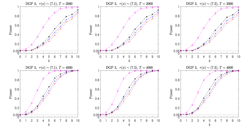
Figure 1: Power across $k$ in DGP 3 for $LM_{T}$ (diamond “$\diamond$” marker) and $Q_{T}(\ell)$ with $\ell=6$ (star “$\ast$” marker), $\ell=9$ (cross “$\times$” marker), and $\ell=12$ (plus “$+$” marker). The horizontal dash-dotted line corresponds to the level $5\%$. Upper Panel: $T=2000$; bottom Panel: $T=4000$.

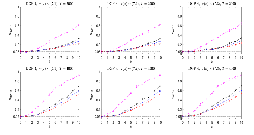
Figure 2: Power across $k$ in DGP 4. The descriptions are as for Fig 1.

From Figs 1–2, we can find that (i) all tests have precise sizes; (ii) the power of all tests becomes large as the value of $T$ or $k$ increases; (iii) $LM_{T}$ is more powerful than all $Q_{\ell}$, and $Q_{6}$ is generally more powerful than $Q_{9}$ and $Q_{12}$; (iv) all tests are more powerful to detect the mis-specification of ARCH part in DGP 3 than the mis-specification of GARCH part in DGP 4; (v) all tests are adaptive, since their power is unaffected by the form of $\tau(x)$. In summary, all tests have a good performance especially for large $T$.

7.4 Comparison with three-step estimation method

In this subsection, we compare the finite-sample performance of $\widehat{\theta}_{T}$ and the three-step estimator $\widecheck{\theta}_{T}$ by investigating their bias difference and efficiency ratio (componentwisely) defined respectively as

$$d(\gamma)=(|\mbox{the Bias of }\widehat{\gamma}_{T}|-|\mbox{the Bias of }\widecheck{\gamma}_{T}|)\times 100\mbox{ and }R(\gamma)=\frac{\mbox{the ESD of }\widehat{\gamma}_{T}}{\mbox{the ESD of }\widecheck{\gamma}_{T}},$$

where $\gamma$ denotes any entry of $\theta_{0}$, and the Bias and ESD of each estimator are computed based on 1000 replications. We calculate the values of $d(\gamma)$ and $R(\gamma)$ under the same simulation settings as in Subsection 7.2, and only report the results for the case of $\tau(x)\sim$ (7.1) in Table 2 due to the adaptiveness of $\widehat{\theta}_{T}$ and $\widecheck{\theta}_{T}$. From Table 2, we can find that (i) both estimators have a comparable bias performance; (ii) when $\eta_{t}\sim N(0,1)$, $\widecheck{\theta}_{T}$ is more (or less) efficient than $\widehat{\theta}_{T}$ in DGP 1 (or DGP 2), indicating that $\widecheck{\theta}_{T}$ does not achieve the semiparametric efficiency bound as indicated in Theorem 5.1; (iii) when $\eta_{t}$ has a heavier distribution (e.g., $\eta_{t}\sim st_{5}$), $\widehat{\theta}_{T}$ exhibits more efficiency advantage over $\widecheck{\theta}_{T}$. In summary, our simulation results suggest that it is unnecessary to further update $\widehat{\theta}_{T}$ to $\widecheck{\theta}_{T}$.

Table 2: The results of $d(\gamma)$ and $R(\gamma)$ based on DGPs 1–2 with $\tau(x)\sim$ (7.1)

		DGP 1: S-ARCH(2)									DGP 2: S-GARCH(1,1)
		$N(0,1)$			$st_{10}$			$st_{5}$			$N(0,1)$			$st_{10}$			$st_{5}$
$T$		$\alpha_{10}$	$\alpha_{20}$		$\alpha_{10}$	$\alpha_{20}$		$\alpha_{10}$	$\alpha_{20}$		$\alpha_{10}$	$\beta_{10}$		$\alpha_{10}$	$\beta_{10}$		$\alpha_{10}$	$\beta_{10}$
2000	$d(\gamma)$	0.08	0.08		-0.23	-0.22		-0.49	-0.53		-0.06	-0.43		-0.05	-0.47		0.04	-0.34
	$R(\gamma)$	1.01	1.02		1.01	0.99		0.46	0.48		0.99	0.94		0.99	0.95		0.89	0.91
4000	$d(\gamma)$	0.05	0.05		-0.13	-0.15		-0.68	-1.15		-0.02	-0.19		-0.02	-0.03		0.02	-0.31
	$R(\gamma)$	1.04	1.04		1.03	1.03		0.40	0.24		0.99	0.96		0.99	0.96		0.97	0.96

7.5 Comparison with the VT method

In this subsection, we compare the finite-sample performance of $\widehat{\theta}_{T}$, $LM_{T}$ and $Q_{T}(\ell)$ with those of $\overline{\theta}_{T}$, $LM_{T}^{vt}$ and $Q_{T}^{vt}(\ell)$, respectively, where $\overline{\theta}_{T}$ defined in (5.3) is the QMLE from the VT method, and $LM_{T}^{vt}$ and $Q_{T}^{vt}(\ell)$ are defined in the same way as $LM_{T}$ and $Q_{T}(\ell)$ with $\widehat{\theta}_{T}$ replaced by $\overline{\theta}_{T}$. Note that when the S-GARCH($p,q$) model is stationary, $\overline{\theta}_{T}$ is asymptotically normal, and $LM_{T}^{vt}$ and $Q_{T}^{vt}(\ell)$ have the same limiting null distributions as those of $LM_{T}$ and $Q_{T}(\ell)$.

First, we compare the efficiency of $\widehat{\theta}_{T}$ and $\overline{\theta}_{T}$ by looking at the following ratio

$$R_{qmle}(\gamma)=\frac{\mbox{the ESD of }\widehat{\gamma}_{T}}{\mbox{the ESD of }\overline{\gamma}_{T}},$$

where the ESD of each estimator is computed based on 1000 replications. Table 3 reports the values of $R_{qmle}(\gamma)$ when the DGP is a stationary S-ARCH(2) (or S-GARCH($1,1$)) model with $\tau(x)\sim(\ref{nochange})$, $\eta_{t}\sim N(0,1)$, and three different choices of $\theta_{0}$. From this table, we find that as expected, all the values of $R_{qmle}(\gamma)$ are close to 1, indicating that $\widehat{\theta}_{T}$ and $\overline{\theta}_{T}$ have the same asymptotic efficiency when the S-GARCH model is stationary.

Table 3: The value of $R_{qmle}(\gamma)$ when the S-GARCH model is stationary

	DGP: S-ARCH(2) with $\tau(x)\sim(\ref{nochange})$ and $\eta_{t}\sim N(0,1)$
	$(\alpha_{10},\alpha_{20})=(0.5,0.1)$			$(\alpha_{10},\alpha_{20})=(0.4,0.2)$			$(\alpha_{10},\alpha_{20})=(0.3,0.3)$
$T$	$R_{qmle}(\alpha_{10})$	$R_{qmle}(\alpha_{20})$		$R_{qmle}(\alpha_{10})$	$R_{qmle}(\alpha_{20})$		$R_{qmle}(\alpha_{10})$	$R_{qmle}(\alpha_{20})$
2000	0.951	1.036		1.043	0.978		1.005	0.997
4000	0.963	1.029		1.007	1.002		1.013	1.005
	DGP: S-GARCH($1,1$) with $\tau(x)\sim(\ref{nochange})$ and $\eta_{t}\sim N(0,1)$
	$(\alpha_{10},\beta_{10})=(0.1,0.8)$			$(\alpha_{10},\beta_{10})=(0.2,0.7)$			$(\alpha_{10},\beta_{10})=(0.3,0.5)$
$T$	$R_{qmle}(\alpha_{10})$	$R_{qmle}(\beta_{10})$		$R_{qmle}(\alpha_{10})$	$R_{qmle}(\beta_{10})$		$R_{qmle}(\alpha_{10})$	$R_{qmle}(\beta_{10})$
2000	1.003	1.022		1.036	1.104		0.995	1.049
4000	0.980	1.089		1.012	1.054		0.971	1.018

Second, we compare the power of $LM_{T}$ and $LM_{T}^{vt}$ and that of $Q_{T}(\ell)$ and $Q_{T}^{vt}(\ell)$ by looking at the following two ratios

$$R_{lm}=\frac{\mbox{the power of }LM_{T}}{\mbox{the power of }LM_{T}^{vt}}\quad\mbox{ and }\quad R_{q}(\ell)=\frac{\mbox{the power of }Q_{T}(\ell)}{\mbox{the power of }Q_{T}^{vt}(\ell)},$$

where the power of each test is computed based on 1000 replications. Table 4 reports the values of $R_{lm}$ and $R_{q}(\ell)$ (for $\ell=6,9$, and $12$), when the data are generated from a stationary S-GARCH($1,2$) model in DGP 3 with $\tau(x)\sim(\ref{nochange})$. The results for DGP 4 are quite similar and hence omitted to save space. From Table 4, we can see that (i) the values of $R_{lm}$ are close to 1 in all examined cases; (ii) when the value of $T$ or $k$ is small, the values of $R_{q}(\ell)$ are slightly less than one, meaning that $Q_{T}^{vt}(\ell)$ could be more powerful than $Q_{T}(\ell)$; (ii) when the value of $T$ or $k$ becomes large, the power advantage of $Q_{T}^{vt}(\ell)$ disappears as the values of $R_{q}(\ell)$ are close to 1. These findings demonstrate that when the S-GARCH model is stationary, our two tests have the same power performance as their counterparts from the VT method especially for large $T$. We also highlight that when the S-GARCH model is non-stationary, our unreported results show that $LM^{vt}_{T}$ and $Q_{T}^{vt}(\ell)$ can cause a severe over-sized problem, and hence they can not be used in this case.

Table 4: The values $R_{lm}$ and $R_{q}(\ell)$ based on a stationary S-GARCH($1,2$) model in DGP 3

		0	1	2	3	4	5	6	7	8	9	10
$R_{lm}$	2000	1.019	1.162	1.081	1.029	1.018	0.997	0.996	0.989	0.98	0.981	0.991
	4000	0.981	1.123	1.027	0.995	0.981	0.989	1.007	1.001	1.000	1.000	1.000
$R_{q}(6)$	2000	1.232	1.019	0.761	0.852	0.916	0.956	1.073	0.987	0.987	0.959	0.988
	4000	1.184	0.889	0.799	0.810	0.907	0.919	0.962	0.968	0.991	0.995	0.999
$R_{q}(9)$	2000	1.282	0.843	0.798	0.943	0.990	0.961	1.0346	0.979	0.993	0.951	0.983
	4000	1.021	1.036	0.754	0.839	0.899	0.903	0.940	0.971	0.985	0.9997	0.996
$R_{q}(12)$	2000	1.160	0.698	0.833	0.916	1.053	0.870	1.021	0.990	0.979	0.963	0.982
	4000	1.056	1.087	0.765	0.880	0.906	0.908	0.955	0.976	0.950	0.991	0.999

8 Applications

In this section, we re-study the US dollar to Indian rupee (USD/INR) exchange rate series and FTSE-index series in Truquet (2017), with respect to in-sample fitting and out-of-sample prediction.

8.1 USD/INR exchange rate

This subsection considers the USD/INR exchange rate series from December 19th, 2005 to February 18th, 2015. The log returns (in percentage) of this series having $T=2301$ observations in total are denoted by $\{y_{t}\}$, and they are plotted in the upper panel of Fig 3. We apply the non-parametric strict stationarity test in Hong et al. (2017) (with the same settings as in their simulation) to $\{y_{t}\}$ and find this test statistic has a p-value close to zero, indicating a strong evidence against the strict stationarity. Thus, using a non-stationary model to fit this series seems appropriate. In Truquet (2017), this return series is fitted by a semiparametric ARCH(1) model with a time-varying intercept and a constant lag-1 ARCH parameter. Motivated by this, we use an ARCH(1) model as the pilot model in Algorithm 7.1 to choose the bandwidth $h=0.0358$, and then calculate the series $\{\widehat{u}_{t}\}$. Based on $\{\widehat{u}_{t}\}$, the BIC selects $p=q=1$ for the S-GARCH model, and hence we fit this return series by the S-GARCH($1,1$) model with $\widehat{\alpha}_{1T}=0.0762_{(0.0231)}$, $\widehat{\beta}_{1T}=0.8443_{(0.0475)}$, and $\widehat{\tau}_{t}$ being plotted in the middle panel of Fig 3, where the values in parentheses are the asymptotic standard errors, and the bandwidth $h=0.0833$ is re-chosen by using a GARCH($1,1$) model as the pilot model in Algorithm 7.1. For this fitted S-GARCH($1,1$) model, the p-values of the portmanteau tests $Q_{T}(6)$, $Q_{T}(9)$, and $Q_{T}(12)$ are 0.6472, 0.7530, and 0.8268, respectively, implying that our fitted short run GARCH($1,1$) component is adequate. In view of the plot of $\{\widehat{\tau}_{t}\}$ in Fig 3, we can find that the long run component $\tau_{t}$ has relatively larger values around years 2009 and 2014. Moreover, we also plot the estimated volatilities based on either S-GARCH or GARCH model in the bottom panel of Fig 3, from which we can see that compared with the S-GARCH model, the GARCH model tends to underestimate the volatilities during 2008-2009 and 2013-2014, and overestimate the volatilities during other periods.

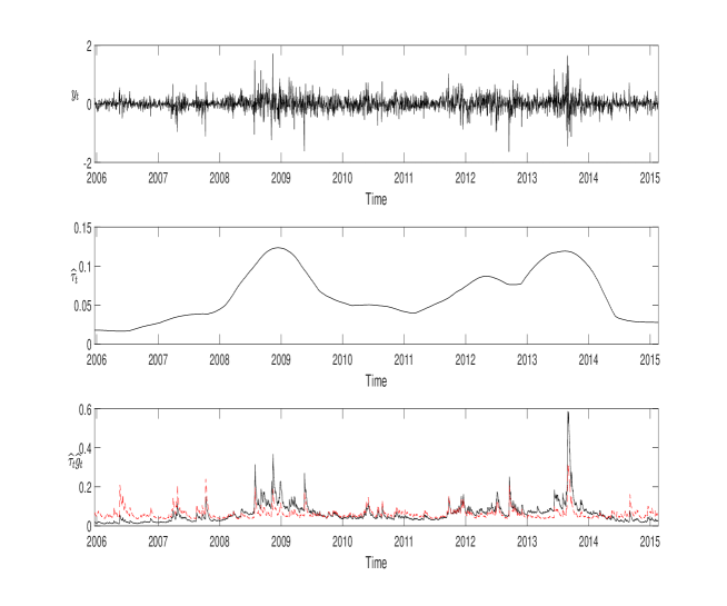
Figure 3: The plot of log returns $\{y_{t}\}$ (upper panel), estimated long-run components $\{\widehat{\tau}_{t}\}$ (middle panel), and estimated volatilities $\{\widehat{\tau}_{t}\widehat{g}_{t}\}$ (bottom panel) based on S-GARCH model (solid line) and GARCH model (dotted line) for USD/INR series. Here, $\widehat{\tau}_{t}$ is computed by using the Epanechnikov kernel with $h=0.0833$ for the S-GARCH model, and $\widehat{\tau}_{t}\equiv\overline{\tau}_{T}$ and $\widehat{g}_{t}=\overline{g}_{t}(\overline{\theta}_{T})$ in (5.3) for the GARCH model.

8.2 FTSE-index

This subsection considers the FTSE-index series from January 4th, 2005 to March 4th, 2015. We study the log returns of this index series with $T=2568$ observations in total, which is denoted by $\{y_{t}\}$ and plotted in the upper panel of Fig 4. As the previous example, we use the non-parametric strict stationarity test in Hong et al. (2017) to $\{y_{t}\}$, and find a strong evidence (with the p-value close to zero) against the strict stationarity. Since Truquet (2017) suggested a semiparametric ARCH(5) model with a time-varying intercept and constant ARCH parameters to fit this return series, we take an ARCH(5) model as the pilot model in Algorithm 7.1, and then select the bandwidth $h=0.0865$ as a result. Based on this choice of $h$, we compute $\{\widehat{u}_{t}\}$ and select $p=q=1$ according to the BIC. Hence, we fit this return series by the S-GARCH($1,1$) model with $\widehat{\alpha}_{1T}=0.1098_{(0.0165)}$, $\widehat{\beta}_{1T}=0.8433_{(0.0233)}$, and $\widehat{\tau}_{t}$ being plotted in the middle panel of Fig 4, where the bandwidth $h=0.0941$ is re-chosen by using a S-GARCH($1,1$) model as the pilot model in Algorithm 7.1. Further, the portmanteau tests $Q_{T}(6)$, $Q_{T}(9)$, and $Q_{T}(12)$ (with p-values equal to $0.5326$, $0.5335$, and $0.2800$, respectively) suggest that this fitted short run GARCH($1,1$) component is adequate. From the middle panel of Fig 4, we find that the long run component $\tau_{t}$ for the FTSE return series only has a clear peak around 2009. This may imply that the stock market index series has a different long run structure with the exchange rate series. Moreover, we also plot the estimated volatilities based on either S-GARCH or GARCH model in the bottom panel of Fig 4, from which we can see that the estimated volatilities from two models are quite close except around years 2008-2009, during which the GARCH model tends to underestimate the volatilities.

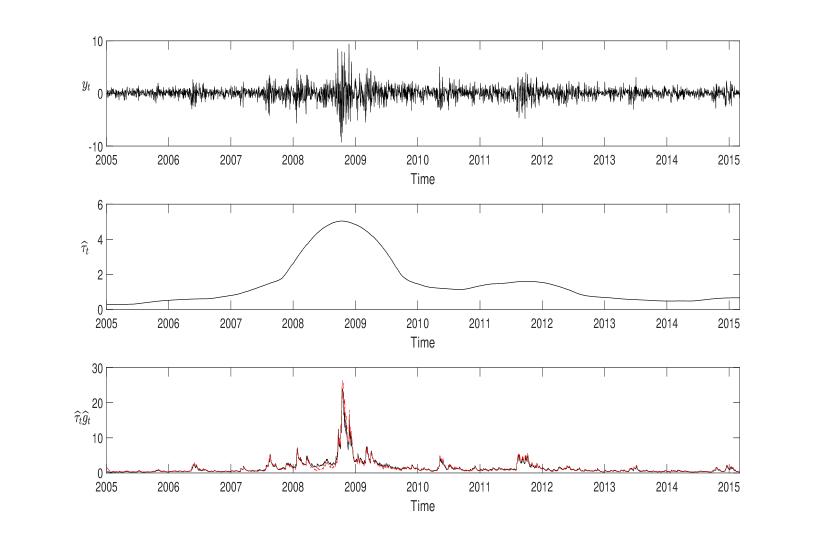
Figure 4: The plots for FTSE series with the same descriptions as in Fig 3. Here, $\widehat{\tau}_{t}$ is computed by using the Epanechnikov kernel with $h=0.0941$ for the S-GARCH model.

8.3 Forecasting comparisons

This subsection makes a forecasting comparison among S-GARCH($1,1$) model, S-ARCH($q$) model, GARCH($1,1$) model in Bollerslev (1986), and LS-ARCH($q$) model (i.e., the locally stationary ARCH($q$) model) in Fryzlewicz et al. (2008) for the USD/INR and FTSE return series. Note that the S-ARCH($q$) model can locally approximate the semiparametric ARCH($q$) model in Truquet (2017), where $q=1$ (or 5) is suggested for the USD/INR (or FTSE) return series. Hence, we follow Truquet (2017) to select $q$ for the S-ARCH($q$) and LS-ARCH($q$) models.

Next, we compare all four models in terms of the averaged QLIKE loss function in Patton (2011). Specifically, we use the in-sample data $\{y_{t}\}_{t=1}^{T_{0}}$ to make a $t_{0}$-step ahead forecast $\widehat{y}_{{T_{0}}+t_{0}|T_{0}}^{2}$ for the out-of-sample data point $y_{T_{0}+t_{0}}^{2}$, and then compute the averaged QLIKE by

$$\mbox{QLIKE}(t_{0})=\frac{1}{T-t_{0}-1499}\sum_{T_{0}=1500}^{T-t_{0}}\log\widehat{y}_{{T_{0}}+t_{0}|T_{0}}^{2}+\frac{y_{T_{0}+t_{0}}^{2}}{\widehat{y}_{{T_{0}}+t_{0}|T_{0}}^{2}}.$$

The model with the smaller value of $\mbox{QLIKE}(t_{0})$ has the better $t_{0}$-step ahead forecasting performance.

Moreover, we introduce how each model computes $\widehat{y}_{{T_{0}}+t_{0}|T_{0}}^{2}$. For the S-GARCH($1,1$) model, we fit the model via the two-step estimation based on the in-sample data $\{y_{t}\}_{t=1}^{T_{0}}$, where the bandwidth $h$ is chosen by Algorithm 7.1 with a pilot GARCH(1, 1) model. With the kernel estimate $\widehat{\tau}_{T_{0}}$ and QMLE $\widehat{\theta}_{T_{0}}$, we then obtain $\widehat{y}_{T_{0}+t_{0}|T_{0}}^{2}=\widehat{\tau}_{T_{0}}g_{T_{0}+t_{0}|T_{0}}(\widehat{\theta}_{T_{0}})$, where $g_{T_{0}+t_{0}|T_{0}}(\widehat{\theta}_{T_{0}})$ computed as for volatility prediction in the GARCH($1,1$) model is the $t_{0}$-step ahead prediction of $g_{T_{0}+t_{0}}$. A similar way is used for the S-ARCH($q$) model to compute $\widehat{y}_{{T_{0}}+t_{0}|T_{0}}^{2}$. For the GARCH($1,1$) model, we fit the model via the VT estimation based on the in-sample data $\{y_{t}\}_{t=1}^{T_{0}}$, and then compute $\widehat{y}_{{T_{0}}+t_{0}|T_{0}}^{2}$ in the conventional way. For the LS-ARCH($q$) model, we follow the method in Fryzlewicz et al. (2008) to compute $\widehat{y}_{{T_{0}}+t_{0}|T_{0}}^{2}$. That is, we treat the last $\widetilde{T}$ in-sample data points as if they came from a stationary ARCH($q$) process, and then estimate the parameters based on these $\widetilde{T}$ data points and compute $\widehat{y}_{{T_{0}}+t_{0}|T_{0}}^{2}$ as for the stationary ARCH($q$) model. Here, the tuning parameter $\widetilde{T}$ is chosen by minimizing the QLIKE, i.e.,

$$\widetilde{T}=\arg\min_{T\in\mathcal{T}}\sum_{t\in[{T_{0}}-50,\,{T_{0}}-1]}\log\widehat{y}_{t+1|t}^{2}(T)+\frac{y_{t+1}^{2}}{\widehat{y}_{t+1|t}^{2}(T)},$$

where $\mathcal{T}=\{50,100,...,500\}$, and $\widehat{y}_{t+1|t}^{2}(T)$ computed as for the stationary ARCH($q$) model is the prediction of $y_{t+1}^{2}$ based on the data $\{y_{i}\}_{i=t-T+1}^{t}$.

Table 5 reports the values of QLIKE($t_{0}$) for all four models, where the prediction horizon $t_{0}$ is taken as $1,5,10$, and $22$, corresponding to daily, weekly, biweekly, and monthly predictions, respectively. The DM test in Diebold and Mariano (1995) is implemented to compare the forecasting accuracy between the model with smallest value of QLIKE and other three models. From this table, we find that for both series, the S-GARCH model has the smallest value of QLIKE for $t_{0}=1$ and 5, while the GARCH model has the smallest value of QLIKE for $t_{0}=10$ and 22. In terms of DM test, we find that the model with smallest value of QLIKE does not exhibit significantly forecasting accuracy than its three competitors for USD/INR series, while it has significantly forecasting accuracy than two ARCH-type competitors for FTSE series. These findings are consistent with those in Fryzlewicz et al. (2008) and Truquet (2017) that (S-)GARCH models could deliver better forecasts than LS-ARCH and S-ARCH models. For the S-GARCH model, we simply just use the latest in-sample long-run component estimator $\widehat{\tau}_{T_{0}}$ to predict the out-of-sample long-run component $\tau_{T_{0}+t_{0}}$. So far, we do not know how to find an “optimal” way under certain criterion to predict $\tau_{T_{0}+t_{0}}$, and this dilemma seems to exist in most of nonparametric methods. We believe that with a better prediction of $\tau_{T_{0}+t_{0}}$, our S-GARCH model could deliver better prediction performances especially at longer prediction horizons.

Table 5: The values of QLIKE($t_{0}$) for $t_{0}=1,5,10$ and 22

	USD/INR					FTSE
	1	5	10	22		1	5	10	22
S-GARCH	$-\bf{1.6981}$	-$\bf{1.6541}$	-1.6050	-1.5479		$\bf{0.7033}$	$\bf{0.7600}$	$0.8179^{*}$	$0.8771^{*}$
S-ARCH	-1.6863	-1.6273	-1.6175	-1.5641		$0.7310^{*}$	$0.7867^{*}$	$0.8304^{*}$	$0.8926^{*}$
GARCH	-1.6815	-1.6520	-$\bf{1.6180}$	-$\bf{1.5774}$		0.7043	0.7665	$\bf{0.7982}$	$\bf{0.8321}$
LS-ARCH	-1.6710	-1.6212	-1.6155	-1.5722		$0.7520^{*}$	$0.7861^{*}$	$0.8058^{*}$	$0.8635^{*}$

• Note: For each $t_{0}$, the smallest value of QLIKE($t_{0}$) among all four models is in boldface.

• DM test is implemented between the model with smallest value of QLIKE($t_{0}$) and other three models, where the symbol star (*) indicates the significance at 5% level.

9 Concluding remarks

This paper provides a complete statistical inference procedure for the S-GARCH model. Our methodologies including the estimation and testing focus on the QMLE of non-time-varying parameters in GARCH-type short run component. Since this QMLE is based on the estimate of the long run component, we develop new proof techniques to derive its asymptotic normality, and find that its asymptotic variance is adaptive to the long run component with unknown form. By comparing the results with those in Hafner and Linton (2010), we find a much simpler asymptotic variance expression for the QMLE, bringing the convenience of use to practitioners. By comparing with the QMLE from the VT method in Francq et al. (2011), we find that our QMLE not only enjoys a broader application scope to deal with the non-stationary S-GARCH model, but also avoids any efficiency loss when the S-GARCH model is stationary. All of these interesting features have not been unveiled before in the literature, and they make our QMLE and its related Lagrange multiplier and portmanteau tests more appealing in practice.

Finally, we suggest some future research topics. First, it is interesting to extend our study to the robust estimation context. This could give us more efficient estimators and more powerful tests for dealing with heavy-tailed data. Second, a similar semiparametric framework as (1.1) can be posed into many variants of the standard GARCH model (e.g., the asymmetric power-GARCH model in Pan et al. (2008) and the asymmetric log-GARCH model in Francq et al. (2013)), and our methodologies could be applied to these new resulting semiparametric models. Third, another possible work is to relax the smooth condition of the long run component to allow for abrupt changes. This seems challenging and may require more non-trivial technical treatments.

Appendix: Proofs

To facilitate the proofs, we first introduce some notations. As for $g_{t}(\theta)$, $\widehat{g}_{t}(\theta)$, $L_{T}(\theta)$, and $\widehat{L}_{T}(\theta)$ in (2.4)–(2.6), we similarly define

$$\widetilde{L}_{T}(\theta)=\sum_{t=1}^{T}\widetilde{l}_{t}(\theta)\quad\text{with}\quad\widetilde{l}_{t}(\theta)=\frac{u_{t}^{2}}{\widetilde{g}_{t}(\theta)}+\log\widetilde{g}_{t}(\theta),$$ (.1)

where $\widetilde{g}_{t}(\theta)$ is defined in the same way as $\widehat{g}_{t}(\theta)$ in (2.6) with $\widehat{u}_{t}$ replaced by $u_{t}$. Meanwhile, we let $\kappa_{T}=\sqrt{(\log T)/(Th)}+h^{2}$, $\Delta_{t}=\widehat{u}^{2}_{t}-u^{2}_{t}$, $\widetilde{S}_{t}(\theta)={\widehat{g}_{t}(\theta)}^{-1}-{\widetilde{g}_{t}(\theta)}^{-1}$, $B^{(j)}$ be a $p\times p$ matrix with $(1,j)$th element 1 and other elements 0, and

$$B=\left(\begin{matrix}\beta_{1}&\beta_{2}&\cdots&\beta_{p}\\ 1&0&\cdots&0\\ \vdots&&&\vdots\\ 0&\cdots&1&0\end{matrix}\right)_{p\times p}.$$

Also, we let $C$ be a generic constant which may differ at each appearance.

Next, we give five technical lemmas, whose proofs are given in the supplementary material (Jiang et al. (2020b)). Lemma .1 captures the error from the nonparametric estimation. Lemma .2 gives some useful results on $\Delta_{t}$ and $\widetilde{S}_{t}(\theta)$. Lemma .3 ensures that replacing $u_{t}$ by $\widehat{u}_{t}$ has a negligible impact on our asymptotic results. Lemma .4 guarantees that the effect from initial values to our asymptotics is negligible. Lemma .5 provides a useful $\beta$-mixing result.

Lemma .1.

Suppose Assumptions 2.1–2.4 hold. Then, almost surely $(a.s.)$,

$\mathrm{(i)}$ ${\displaystyle\sup_{x\in(0,1)}\Big{|}\widehat{\tau}(x)-\tau(x)-\frac{1}{T}\sum_{t=1}^{T}K_{h}\Big{(}x-\frac{t}{T}\Big{)}\tau(x)(u^{2}_{t}-1)-h^{2}b(x)\Big{|}=O\Big{(}\frac{\log T}{Th}\Big{)}+o(h^{2})}$;

$\mathrm{(ii)}$ ${\displaystyle\sup_{x\in(0,1)}\Big{|}\frac{1}{T}\sum_{t=1}^{T}K_{h}\Big{(}x-\frac{t}{T}\Big{)}\tau(x)(u^{2}_{t}-1)\Big{|}=O\Big{(}\sqrt{\frac{\log T}{Th}}\Big{)}}$.

Lemma .2.

Suppose the conditions in Theorem 2.2 hold. Then,

$(\mathrm{i})$ $\Delta_{t}={\tau_{t}}^{-1}{(\tau_{t}-\widehat{\tau}_{t})u^{2}_{t}}+O(\kappa_{T}^{2})u^{2}_{t}$, where $O(1)$ holds uniformly in $t$;

$(\mathrm{ii})$ $\sup_{\theta\in\Theta}|\widetilde{S}_{t}(\theta)|\leq C\kappa_{T}$.

Lemma .3.

Suppose the conditions in Theorem 2.2 hold. Then, for any $\iota\leq 4(1+2\delta)$,

$(\mathrm{i})$ ${\displaystyle\sup_{\theta\in\Theta}\Big{\|}\widehat{g}_{t}(\theta)-\widetilde{g}_{t}(\theta)\Big{\|}_{\iota}\leq C\kappa_{T}}$;

$(\mathrm{ii})$ ${\displaystyle\sup_{\theta\in\Theta}\Big{\|}\frac{\partial\widehat{g}_{t}(\theta)}{\partial\theta}-\frac{\partial\widetilde{g}_{t}(\theta)}{\partial\theta}\Big{\|}_{\iota}\leq C\kappa_{T}}$;

$(\mathrm{iii})$ ${\displaystyle\sup_{\theta\in\Theta}\Big{\|}\frac{\partial^{2}\widehat{g}_{t}(\theta)}{\partial\theta\partial\theta^{\prime}}-\frac{\partial^{2}\widetilde{g}_{t}(\theta)}{\partial\theta\partial\theta^{\prime}}\Big{\|}_{\iota}\leq C\kappa_{T}}$.

Lemma .4.

Suppose Assumptions 2.1 and 2.5–2.7 hold. Then, there exists a $\rho\in(0,1)$ such that for any $\iota\leq 4(1+2\delta)$,

$(\mathrm{i})$ ${\displaystyle\sup_{\theta\in\Theta}\Big{\|}g_{t}(\theta)-\widetilde{g}_{t}(\theta)\Big{\|}_{\iota}\leq C\rho^{t}}$;

$(\mathrm{ii})$ ${\displaystyle\sup_{\theta\in\Theta}\Big{\|}\frac{\partial g_{t}(\theta)}{\partial\theta}-\frac{\partial\widetilde{g}_{t}(\theta)}{\partial\theta}\Big{\|}_{\iota}\leq C\rho^{t}}$;

$(\mathrm{iii})$ ${\displaystyle\sup_{\theta\in\Theta}\Big{\|}\frac{\partial^{2}g_{t}(\theta)}{\partial^{2}\theta\partial\theta^{\prime}}-\frac{\partial^{2}\widetilde{g}_{t}(\theta)}{\partial\theta\partial\theta^{\prime}}\Big{\|}_{\iota}\leq C\rho^{t}}$.

Lemma .5.

Suppose Assumptions 2.4–2.5 and 2.7(i) hold. Then, $\big{\{}(u_{t},g_{t},\frac{\partial g_{t}(\theta_{0})}{\partial\theta^{\prime}})\big{\}}$ is strictly stationary and $\beta$-mixing with exponential decay.

Proof of Theorem 2.1. See the supplementary material in Jiang et al. (2020b). ∎

Proof of Theorem 2.2($\mathrm{i}$). See the supplementary material in Jiang et al. (2020b).

In order to prove Theorem 2.2($\mathrm{ii}$), we need a crucial proposition, which is interesting in its own right.

Proposition .1.

Let $\{c_{t}\}_{t\in\mathbb{Z}}$ be a sequence of stationary process and $\mathcal{F}_{t}^{s}=\sigma(c_{i},t\leq i\leq s)$ be the sigma-filed generated by $\{c_{i},t\leq i\leq s\}$. Define

$$S_{T}=\frac{1}{\sqrt{T}}\sum_{t=1}^{T}b_{t}\Big{\{}\frac{1}{Th}\sum_{s=1}^{T}K\Big{(}\frac{s-t}{Th}\Big{)}a_{s}\Big{\}},$$

where $a_{t}=f(c_{t})$, $b_{t}=g(c_{t},c_{t-k})$ for some $k\leq n_{T}$, and $f(\cdot)$ and $g(\cdot,\cdot)$ are two real-valued functions. Suppose the following conditions hold:

$(1)$ $Ea_{t}=0$, $Eb_{t}=0$, $E|a_{t}|^{\iota_{1}(1+2\delta)}<\infty$ and $E|b_{t}|^{\iota_{2}(1+2\delta)}<\infty$, where $\iota_{1},\iota_{2}>0$ satisfy $\iota_{1}^{-1}+\iota_{2}^{-1}=1/2$ and $\delta>0$;

$(2)$ $c_{t}$ is $\beta$-mixing with mixing coefficients $\beta(j)$ satisfying $\sum_{j=1}^{\infty}\beta(j)^{\delta/(1+\delta)}<\infty$;

$(3)$ $K(\cdot)$ satisfies Assumption 2.3 and $h$ satisfies Assumption 2.8;

$(4)$ $n_{T}$ is either a constant or $n_{T}\to\infty$ and $n_{T}=o(\sqrt{Th^{2}})$ as $T\to\infty$.

Then,

$$(\mathrm{i})~{}|ES_{t}|\leq\frac{Cn_{T}}{\sqrt{T}h}\quad\text{and}\quad(\mathrm{ii})~{}ES_{T}^{2}\leq C\max\Big{\{}\frac{n_{T}}{\sqrt{Th}},\frac{1}{Th^{2}}\Big{\}}.$$

Proof.

We decompose $S_{T}=S_{T,1}+S_{T,2}+S_{T,3}+S_{T,4}$, where

$$S_{T,1}= \frac{1}{T^{3/2}h}\sum_{t=1}^{T-1}b_{t}\sum_{s=t+1}^{T}K\Big{(}\frac{s-t}{Th}\Big{)}a_{s},\quad S_{T,2}=\frac{1}{T^{3/2}h}\sum_{t=n_{T}+1}^{T}b_{t}\sum_{s=1}^{t-n_{T}}K\Big{(}\frac{s-t}{Th}\Big{)}a_{s},$$

$$S_{T,3}= \frac{1}{T^{3/2}h}\sum_{t=n_{T}+1}^{T-1}b_{t}\sum_{s=t-n_{T}+1}^{t}K\Big{(}\frac{s-t}{Th}\Big{)}a_{s},\quad S_{T,4}=\frac{1}{T^{3/2}h}\sum_{t=1}^{n_{T}}b_{t}\sum_{s=1}^{t}K\Big{(}\frac{s-t}{Th}\Big{)}a_{s}.$$

$(\mathrm{i})$ Under Condition (1), we have that $\iota_{1}>2$ and $\iota_{2}>2$, which indicate $\|a_{t}\|_{2(1+2\delta)}<\infty$ and $\|b_{t}\|_{2(1+2\delta)}<\infty$. Since $b_{t}\in\mathcal{F}_{t-n_{T}}^{t}$, by Conditions (1)–(3) and Davydov’s inequality (see Davydov (1968)), we have

$$|ES_{T,1}|\leq \frac{C}{T^{3/2}h}\sum_{t=1}^{T-1}\sum_{s=t+1}^{T}|E(b_{t}a_{s})|$$

$$\leq \frac{C}{T^{3/2}h}\sum_{t=1}^{T-1}\sum_{s=t+1}^{T}\beta(s-t)^{\delta/(1+\delta)}\|b_{t}\|_{2(1+\delta)}\|a_{s}\|_{2(1+\delta)}=\frac{C}{T^{1/2}h}.$$

Similarly, we can show that $|ES_{T,2}|\leq\frac{C}{T^{1/2}h}$. The result holds by noticing that

$$E|S_{T,3}|\leq\frac{C}{T^{3/2}h}\sum_{t=n_{T}+1}^{T-1}\sum_{s=t-n_{T}+1}^{t}E|b_{t}a_{s}|\leq\frac{Cn_{T}}{T^{1/2}h},$$

$$E|S_{T,4}|\leq\frac{C}{T^{3/2}h}\sum_{t=1}^{n_{T}}\sum_{s=1}^{t}E|b_{t}a_{s}|\leq\frac{Cn_{T}^{2}}{T^{3/2}h}.$$

$(\mathrm{ii})$ It is not hard to obtain that $ES_{T,3}^{2}\leq\frac{Cn_{T}^{2}}{Th^{2}}$ and $ES_{T,4}^{2}\leq\frac{Cn_{T}^{4}}{T^{3}h^{2}}$. Below, we only prove that $ES_{T,1}^{2}\leq\frac{Cn_{T}}{\sqrt{Th}}+\frac{C}{Th^{2}}$, since we can similarly show that $ES_{T,2}^{2}\leq\frac{C}{\sqrt{Th}}+\frac{C}{Th^{2}}$.

Let $\varpi_{t}=\sum_{s=t+1}^{T}K(\frac{t-s}{Th})a_{s}$. Then, $ES_{T,1}^{2}=\frac{1}{T^{3}h^{2}}\sum_{t=1}^{T}\sum_{t^{\prime}=1}^{T}Eb_{t}b_{t^{\prime}}\varpi_{t}\varpi_{t^{\prime}}:=V_{T,1}+V_{T,2}+V_{T,3}$, where

$$V_{T,1}= \frac{1}{T^{3}h^{2}}\sum_{t=1}^{T}\sum_{t^{\prime}=t+1}^{T}Eb_{t}b_{t^{\prime}}\varpi_{t}\varpi_{t^{\prime}},\quad V_{T,2}=\frac{1}{T^{3}h^{2}}\sum_{t=1}^{T}E(b_{t}\varpi_{t})^{2},$$

$$V_{T,3}= \frac{1}{T^{3}h^{2}}\sum_{t^{\prime}=1}^{T}\sum_{t=t^{\prime}+1}^{T}Eb_{t}b_{t^{\prime}}\varpi_{t}\varpi_{t^{\prime}}.$$

For simplicity, we only show that $V_{T,1}\leq\frac{Cn_{T}}{\sqrt{Th}}+\frac{C}{Th^{2}}$. Let

$$\varpi_{1t}= \sum_{s=t+1}^{t^{\prime}}K\Big{(}\frac{t-s}{Th}\Big{)}a_{s}\in\mathcal{F}_{t+1}^{\min\{t^{\prime}-1,t+[Th]\}},\quad\varpi_{2t}=\sum_{s=t^{\prime}+1}^{T}K\Big{(}\frac{t-s}{Th}\Big{)}a_{s}\in\mathcal{F}_{t^{\prime}}^{\infty},$$

$$\varpi_{1t^{\prime}}= \sum_{s=t^{\prime}+1}^{t^{\prime}+[Th]-1}K\Big{(}\frac{t^{\prime}-s}{Th}\Big{)}a_{s}\in\mathcal{F}_{t^{\prime}}^{t^{\prime}+[Th]-1},\quad\varpi_{2t^{\prime}}=\sum_{s=t^{\prime}+[Th]}^{T}K\Big{(}\frac{t^{\prime}-s}{Th}\Big{)}a_{s}\in\mathcal{F}_{t^{\prime}+[Th]}^{\infty}.$$

Here, we have used the fact that $K(\frac{t-s}{Th})=0$ if $|t-s|>[Th]$ by Condition (3). Moreover, decompose $V_{T,1}=V_{T,11}+V_{T,12}+V_{T,13}$, where

$$V_{T,11}= \frac{1}{T^{3}h^{2}}\sum_{t=1}^{T}\sum_{t^{\prime}=t+1}^{T}Eb_{t}\varpi_{1t}b_{t^{\prime}}\varpi_{1t^{\prime}},\quad V_{T,12}=\frac{1}{T^{3}h^{2}}\sum_{t=1}^{T}\sum_{t^{\prime}=t+1}^{T}Eb_{t}\varpi_{1t}b_{t^{\prime}}\varpi_{2t^{\prime}},$$

$$V_{T,13}= \frac{1}{T^{3}h^{2}}\sum_{t=1}^{T}\sum_{t^{\prime}=t+1}^{T}Eb_{t}\varpi_{2t}b_{t^{\prime}}\varpi_{t^{\prime}}.$$

Using Lemmas .6–.8 below, it follows that $V_{T,1}\leq C\max\big{\{}\frac{n_{T}}{\sqrt{Th}},\frac{1}{Th^{2}}\big{\}}$. ∎

Lemma .6.

Under the conditions in Proposition .1, $V_{T,11}\leq C\max\big{\{}\frac{1}{\sqrt{Th}},\frac{1}{Th^{2}}\big{\}}$.

Proof.

First, we decompose $V_{T,11}=\sum_{i=1}^{3}V_{T,11i}$, where

$$V_{T,111}= \frac{1}{T^{3}h^{2}}\sum_{t=1}^{T}\sum_{t^{\prime}=t+1}^{t+2[Th]}\mathrm{Cov}(b_{t}\varpi_{1t}b_{t^{\prime}},\varpi_{1t^{\prime}}),V_{T,112}=\frac{1}{T^{3}h^{2}}\sum_{t=1}^{T}\sum_{t^{\prime}=t+2[Th]+1}^{T}\mathrm{Cov}(b_{t}\varpi_{1t},b_{t^{\prime}}\varpi_{1t^{\prime}}),$$

$$V_{T,113}= \frac{1}{T^{3}h^{2}}\sum_{t=1}^{T}\sum_{t^{\prime}=t+2[Th]+1}^{T}E(b_{t}\varpi_{1t})E(b_{t^{\prime}}\varpi_{1t^{\prime}}).$$

Next, by Theorem 4.1 in Shao and Yu (1996), we have

$$\|\varpi_{1t}\|_{\iota}\leq C\sqrt{\min\{t^{\prime}-t-1,[Th]+1\}}\|a_{s}\|_{\iota+\xi_{0}}$$ (.2)

for some $0\leq\iota\leq\iota_{1}(1+2\delta)-\xi_{0}$ and $\xi_{0}>0$. Since $b_{t}\varpi_{1t}b_{t^{\prime}}\in\mathcal{F}_{-\infty}^{t^{\prime}}$, by Davydov’s inequality and Hölder’s inequality, we can obtain

$$|V_{T,111}|\leq \frac{1}{T^{3}h^{2}}\sum_{t=1}^{T}\sum_{t^{\prime}=t+1}^{t+2[Th]}\sum_{s=t^{\prime}}^{t^{\prime}+[Th]-1}C\beta(s-t^{\prime})^{\delta/(1+\delta)}\|b_{t}\varpi_{1t}b_{t^{\prime}}\|_{(1+\delta)\iota_{1}/(\iota_{1}-1)}\|a_{s}\|_{\iota_{1}(1+\delta)}$$

$$\leq \frac{1}{T^{3}h^{2}}\sum_{t=1}^{T}\sum_{t^{\prime}=t+1}^{t+2[Th]}\sum_{s=t^{\prime}}^{t^{\prime}+[Th]-1}C\beta(s-t^{\prime})^{\delta/(1+\delta)}\|b_{t}\|^{2}_{\iota_{2}(1+\delta)}\|\varpi_{1t}\|_{\iota_{1}(1+\delta)}\|a_{s}\|_{\iota_{1}(1+\delta)}$$

$$= \frac{1}{T^{3}h^{2}}\sum_{t=1}^{T}\sum_{t^{\prime}=t+1}^{t+2[Th]}\|\varpi_{1t}\|_{\iota_{1}(1+\delta)}.$$

Using (.2) with $\iota=\iota_{1}(1+\delta)$ and $\xi_{0}=\iota_{1}\delta$, it follows that $|V_{T,111}|\leq\frac{CT^{2}h\sqrt{Th}}{T^{3}h^{2}}=\frac{C}{\sqrt{Th}}$.

Third, we note that $b_{t}\varpi_{1t}\in\mathcal{F}_{-\infty}^{t+[Th]}$ as $t^{\prime}>t+[Th]$, and $b_{t^{\prime}}K(\frac{t^{\prime}-s}{Th})a_{s}\in\mathcal{F}_{t^{\prime}-n_{T}}^{\infty}\subset\mathcal{F}_{t^{\prime}-[Th]+1}^{\infty}$ as $n_{T}\ll[Th]$. Then, by Davydov’s inequality and Hölder’s inequality, we have

$$|V_{T,112}|\leq \frac{1}{T^{3}h^{2}}\sum_{t=1}^{T}\sum_{t^{\prime}=t+2[Th]+1}^{T}\sum_{s=t^{\prime}+1}^{t^{\prime}+[Th]-1}\Big{|}\mathrm{Cov}\big{(}b_{t}\varpi_{1t},b_{t^{\prime}}K\big{(}(t^{\prime}-s)/Th\big{)}a_{s}\big{)}\Big{|}$$

$$\leq \frac{C}{T^{3}h^{2}}\sum_{t=1}^{T}\sum_{t^{\prime}=t+2[Th]+1}^{T}\sum_{s=t^{\prime}+1}^{t^{\prime}+[Th]-1}\beta(t^{\prime}-t-2[Th])^{\delta/(1+\delta)}\|b_{t}\varpi_{1t}\|_{2(1+\delta)}\|b_{t^{\prime}}a_{s}\|_{2(1+\delta)}$$

$$\leq \frac{C}{T^{3}h^{2}}\sum_{t=1}^{T}\sum_{t^{\prime}=t+2[Th]+1}^{T}\sum_{s=t^{\prime}+1}^{t^{\prime}+[Th]-1}\beta(t^{\prime}-t-2[Th])^{\delta/(1+\delta)}\|b_{t}\|^{2}_{\iota_{2}(1+\delta)}\|\varpi_{1t}\|_{\iota_{1}(1+\delta)}\|a_{s}\|_{\iota_{1}(1+\delta)}$$

$$\leq \frac{CTh}{T^{3}h^{2}}\sum_{t=1}^{T}\|\varpi_{1t}\|_{\iota_{1}(1+\delta)}.$$

Using (.2) with $\iota=\iota_{1}(1+\delta)$ and $\xi_{0}=\iota_{1}\delta$, it follows that $|V_{T,112}|\leq\frac{C}{\sqrt{Th}}$. Finally, since it is straightforward to show that $|V_{T,113}|\leq\frac{C}{Th^{2}}$, the result follows. ∎

Lemma .7.

Under the conditions in Proposition .1, $V_{T,12}\leq C/\sqrt{Th}$.

Proof.

Note that $b_{t}\varpi_{1t}b_{t^{\prime}}\in\mathcal{F}_{-\infty}^{t^{\prime}}$. By Davydov’s inequality, Hölder’s inequality and (.2), we have

$$\big{|}\mathrm{Cov}(b_{t}\varpi_{1t}b_{t^{\prime}},\varpi_{2t^{\prime}})\big{|}\leq \sum_{s=t^{\prime}+[Th]}^{T}K\Big{(}\frac{t^{\prime}-s}{Th}\Big{)}\big{|}\mathrm{Cov}(b_{t}\varpi_{1t}b_{t^{\prime}},a_{s})\big{|}$$

$$\leq C\sum_{j=[Th]}^{T}\beta(j)^{\delta/(1+\delta)}\|b_{t}\|^{2}_{\iota_{2}(1+\delta)}\|\varpi_{1t}\|_{\iota_{1}(1+\delta)}\|a_{s}\|_{\iota_{1}(1+\delta)}$$

$$= C\sqrt{Th}\sum_{j=[Th]}^{T}\beta(j)^{\delta/(1+\delta)}.$$

By Condition (2) and the fact $Th\to\infty$ as $T\to\infty$, we have that $Th\sum_{j=[Th]}^{T}\beta(j)^{\delta/(1+\delta)}\leq C$, which entails that $|V_{T,12}|\leq\frac{C}{\sqrt{T^{3}h^{5}}}\leq\frac{C}{\sqrt{Th}}.$ ∎

Lemma .8.

Under assumptions of Proposition .1, $V_{T,13}\leq Cn_{T}/\sqrt{Th}$.

Proof.

Rewrite $\varpi_{t^{\prime}}=\varpi_{3t^{\prime}}+\varpi_{4t^{\prime}}$, where

$$\varpi_{3t^{\prime}}=\sum_{r=t^{\prime}+1}^{s}K\Big{(}\frac{t^{\prime}-r}{Th}\Big{)}a_{r}\mbox{ and }\varpi_{4t^{\prime}}=\sum_{r=s+1}^{t^{\prime}+[Th]}K\Big{(}\frac{t^{\prime}-r}{Th}\Big{)}a_{r}.$$

Then, we can decompose $V_{T,13}=\sum_{i=1}^{4}V_{T,13i}$, where

$$V_{T,131}= \frac{1}{T^{3}h^{2}}\sum_{t=1}^{T}\sum_{t^{\prime}=t+1}^{t+[Th]}\sum_{s=t^{\prime}+1}^{t+[Th]}K\Big{(}\frac{t-s}{Th}\Big{)}\mathrm{Cov}(b_{t}b_{t^{\prime}},a_{s}\varpi_{3t^{\prime}}),$$

$$V_{T,132}= \frac{1}{T^{3}h^{2}}\sum_{t=1}^{T}\sum_{t^{\prime}=t+1}^{t+[Th]}\sum_{s=t^{\prime}+1}^{t+[Th]}K\Big{(}\frac{t-s}{Th}\Big{)}\mathrm{Cov}(b_{t}b_{t^{\prime}},a_{s}\varpi_{4t^{\prime}}),$$

$$V_{T,133}= \frac{1}{T^{3}h^{2}}\sum_{t=1}^{T}\sum_{t^{\prime}=t+1}^{t+[Th]}\sum_{s=t^{\prime}+1}^{t+[Th]}K\Big{(}\frac{t-s}{Th}\Big{)}E(b_{t}b_{t^{\prime}})E(a_{s}\varpi_{t^{\prime}}),$$

$$V_{T,134}= \frac{1}{T^{3}h^{2}}\sum_{t=1}^{T}\sum_{t^{\prime}=t+[Th]+1}^{T}\sum_{s=t^{\prime}+1}^{T}K\Big{(}\frac{t-s}{Th}\Big{)}E(b_{t}b_{t^{\prime}}a_{s}\varpi_{t^{\prime}}).$$

First, by interchanging summations of $s$ and $r$, we have

$$V_{T,131}=\frac{C}{T^{3}h^{2}}\sum_{t=1}^{T}\sum_{t^{\prime}=t+1}^{t+[Th]}\sum_{r=t^{\prime}+1}^{t+[Th]}\sum_{s=r}^{t+[Th]}K\Big{(}\frac{t-s}{Th}\Big{)}K\Big{(}\frac{t^{\prime}-r}{Th}\Big{)}\mathrm{Cov}(b_{t}b_{t^{\prime}},a_{s}a_{r}).$$

Since $b_{t}b_{t^{\prime}}\in\mathcal{F}_{-\infty}^{t^{\prime}}$, by Davydov’s inequality and Hölder’s inequality, we can show

$$|V_{T,131}|\leq \frac{C}{T^{3}h^{2}}\sum_{t=1}^{T}\sum_{t^{\prime}=t+1}^{t+[Th]}\sum_{r=t^{\prime}+1}^{t+[Th]}\mathrm{Cov}\big{(}b_{t}b_{t^{\prime}},a_{r}\sum_{s=r}^{t+[Th]}K\Big{(}\frac{t-s}{Th}\Big{)}a_{s}\big{)}$$

$$\leq \frac{C}{T^{3}h^{2}}\sum_{t=1}^{T}\sum_{t^{\prime}=t+1}^{t+[Th]}\sum_{r=t^{\prime}+1}^{t+[Th]}\beta(r-t^{\prime})^{\delta/(1+\delta)}\|b_{t}b_{t^{\prime}}\|_{\iota_{2}(1+\delta)/2}$$

$$\quad\quad\times\Big{\|}a_{r}\sum_{s=r}^{t+[Th]}K\Big{(}\frac{t-s}{Th}\Big{)}a_{s}\Big{\|}_{\iota_{1}(1+\delta)}$$

$$\leq \frac{C}{T^{3}h^{2}}\sum_{t=k+1}^{T}\sum_{t^{\prime}=t+1}^{t+[Th]}\sum_{r=t^{\prime}}^{t+[Th]}\beta(r-t^{\prime})^{\delta/(1+\delta)}\|b_{t}\|^{2}_{\iota_{2}(1+\delta)/2}$$

$$\quad\quad\times\|a_{r}\|_{\iota_{1}(1+\delta)}\Big{\|}\sum_{s=r}^{t+[Th]}K\Big{(}\frac{t-s}{Th}\Big{)}a_{s}\Big{\|}_{\iota_{1}(1+\delta)}.$$

By similar arguments as for (.2), we have

$$\Big{\|}\sum_{s=r}^{t+[Th]}K\Big{(}\frac{t-s}{Th}\Big{)}a_{s}\Big{\|}_{\iota_{1}(1+\delta)}\leq C\sqrt{t+[Th]-r}\|a_{s}\|_{\iota_{1}(1+2\delta)}\leq C\sqrt{Th}\|a_{s}\|_{\iota_{1}(1+2\delta)},$$

and hence it follows that $|V_{T,131}|\leq\frac{CT^{2}h\sqrt{Th}}{T^{3}h^{2}}=\frac{C}{\sqrt{Th}}$. Similarly, $|V_{T,132}|\leq\frac{C}{\sqrt{Th}}$.

Next, we decompose $V_{T,133}=V_{T,1331}+V_{T,1332}$, where

$$V_{T,1331}= \frac{1}{T^{3}h^{2}}\sum_{t=1}^{T}\sum_{t^{\prime}=t+1}^{t+n_{T}}\sum_{s=t^{\prime}}^{t+[Th]}K\Big{(}\frac{t-s}{Th}\Big{)}E(b_{t}b_{t^{\prime}})E(a_{s}\varpi_{t^{\prime}}),$$

$$V_{T,1332}= \frac{1}{T^{3}h^{2}}\sum_{t=1}^{T}\sum_{t^{\prime}=t+n_{T}+1}^{t+[Th]}\sum_{s=t^{\prime}}^{t+[Th]}K\Big{(}\frac{t-s}{Th}\Big{)}E(b_{t}b_{t^{\prime}})E(a_{s}\varpi_{t^{\prime}}).$$

It is easy to see

$$|V_{T,1331}|\leq \frac{1}{T^{3}h^{2}}\sum_{t=1}^{T}\sum_{t^{\prime}=t+1}^{t+n_{T}}\sum_{s=t^{\prime}}^{t+[Th]}K\Big{(}\frac{t-s}{Th}\Big{)}\|b_{t}\|^{2}_{2}\|a_{s}\|_{2}\|\varpi_{t^{\prime}}\|_{2}\leq\frac{CT^{2}h}{T^{3}h^{2}}\sum_{t^{\prime}=t+1}^{t+n_{T}}\|\varpi_{t^{\prime}}\|_{2}$$

and $\|\varpi_{t^{\prime}}\|_{2}\leq C\sqrt{Th}\|a_{s}\|_{2(1+\delta)}$ by (.2). So, we have that $|V_{T,1331}|\leq Cn_{T}/\sqrt{Th}$. Moreover, by Davydov’s inequality and Hölder’s inequality, we can show

$$|V_{T,1332}|\leq \frac{C}{T^{3}h^{2}}\sum_{t=1}^{T}\sum_{t^{\prime}=t+n_{T}+1}^{t+[Th]}\sum_{s=t^{\prime}}^{t+[Th]}\beta(t^{\prime}-n_{T}-t)^{\delta/(1+\delta)}\|b_{t}\|^{2}_{\iota_{2}(1+\delta)/2}\|a_{s}\|_{2}\|\varpi_{t^{\prime}}\|_{2}$$

$$\leq \frac{CT^{2}h\sqrt{Th}}{T^{3}h^{2}}=\frac{C}{\sqrt{Th}},$$

which implies that $|V_{T,133}|\leq Cn_{T}/\sqrt{Th}$.

Finally, since $K\big{(}\frac{s-t}{Th}\big{)}=0$ when $s\geq t^{\prime}>t+[Th]$, it follows that $V_{T,134}=0$, and hence the result follows. ∎

Proof of Theorem 2.2($\mathrm{ii}$). By Taylor’s expansion, we have

$$\sqrt{T}(\widehat{\theta}_{T}-\theta_{0})=-\Big{\{}\frac{1}{T}\frac{\partial^{2}\widehat{L}_{T}(\theta^{*})}{\partial\theta\partial\theta^{\prime}}\Big{\}}^{-1}\frac{1}{\sqrt{T}}\frac{\partial\widehat{L}_{T}({\theta}_{0})}{\partial\theta},$$ (.3)

where $\theta^{*}$ lies between $\hat{\theta}_{T}$ and $\theta_{0}$.

Let $\widehat{g}_{t}=\widehat{g}_{t}(\theta_{0}),\widehat{g}_{t}=\widehat{g}_{t}(\theta_{0})$, $\frac{\partial\widehat{g}_{t}}{\partial\theta_{m}}=\frac{\partial\widehat{g}_{t}(\theta_{0})}{\partial\theta_{m}}$, $\frac{\partial\widetilde{g}_{t}}{\partial\theta_{m}}=\frac{\partial\widetilde{g}_{t}(\theta_{0})}{\partial\theta_{m}}$, and $\widetilde{S}_{t}=\widetilde{S}_{t}(\theta_{0})$. By noting that $\widehat{g}_{t}^{-1}=\widetilde{S}_{t}+\widetilde{g}_{t}^{-1}$, $\widehat{g}_{t}^{-1}\widehat{u}^{2}_{t}=\widetilde{g}_{t}^{-1}u^{2}_{t}+u^{2}_{t}\widetilde{S}_{t}+\widetilde{g}_{t}^{-1}\Delta_{t}$ and $\frac{\partial\widehat{g}_{t}}{\partial\theta_{m}}=\frac{\partial\widehat{g}_{t}}{\partial\theta_{m}}-\frac{\partial\widetilde{g}_{t}}{\partial\theta_{m}}+\frac{\partial\widetilde{g}_{t}}{\partial\theta_{m}}$, we have

$$\frac{1}{\sqrt{T}}\frac{\partial\widehat{L}_{T}({\theta}_{0})}{\partial\theta_{m}}=\sum_{i=1}^{12}U_{i},$$ (.4)

where

$$U_{1}= \frac{1}{\sqrt{T}}\sum_{t=1}^{T}(1-\widetilde{g}_{t}^{-1}u^{2}_{t}){\widetilde{g}_{t}}^{-1}\frac{\partial\widetilde{g}_{t}}{\partial\theta_{m}},~{}\quad U_{2}=\frac{1}{\sqrt{T}}\sum_{t=1}^{T}(1-\widetilde{g}_{t}^{-1}u^{2}_{t}){\widetilde{g}_{t}}^{-1}\Big{(}\frac{\partial\widehat{g}_{t}}{\partial\theta_{m}}-\frac{\partial\widetilde{g}_{t}}{\partial\theta_{m}}\Big{)},$$

$$U_{3}= \frac{1}{\sqrt{T}}\sum_{t=1}^{T}(1-\widetilde{g}_{t}^{-1}u^{2}_{t})\widetilde{S}_{t}\frac{\partial\widetilde{g}_{t}}{\partial\theta_{m}},\quad\quad U_{4}=\frac{1}{\sqrt{T}}\sum_{t=1}^{T}(1-\widetilde{g}_{t}^{-1}u^{2}_{t})\widetilde{S}_{t}\Big{(}\frac{\partial\widehat{g}_{t}}{\partial\theta_{m}}-\frac{\partial\widetilde{g}_{t}}{\partial\theta_{m}}\Big{)},$$

$$U_{5}= -\frac{1}{\sqrt{T}}\sum_{t=1}^{T}\widetilde{g}_{t}^{-1}u^{2}_{t}\widetilde{S}_{t}\frac{\partial\widetilde{g}_{t}}{\partial\theta_{m}},\qquad\quad U_{6}=-\frac{1}{\sqrt{T}}\sum_{t=1}^{T}\widetilde{g}_{t}^{-1}u^{2}_{t}\widetilde{S}_{t}\Big{(}\frac{\partial\widehat{g}_{t}}{\partial\theta_{m}}-\frac{\partial\widetilde{g}_{t}}{\partial\theta_{m}}\Big{)},$$

$$U_{7}= -\frac{1}{\sqrt{T}}\sum_{t=1}^{T}u^{2}_{t}\widetilde{S}_{t}^{2}\frac{\partial\widetilde{g}_{t}}{\partial\theta_{m}},\qquad\qquad~{}U_{8}=-\frac{1}{\sqrt{T}}\sum_{t=1}^{T}u^{2}_{t}\widetilde{S}_{t}^{2}\Big{(}\frac{\partial\widehat{g}_{t}}{\partial\theta_{m}}-\frac{\partial\widetilde{g}_{t}}{\partial\theta_{m}}\Big{)},$$

$$U_{9}= -\frac{1}{\sqrt{T}}\sum_{t=1}^{T}\Delta_{t}\widehat{g}_{t}^{-1}\widetilde{g}_{t}^{-1}\frac{\partial\widetilde{g}_{t}}{\partial\theta_{m}},\qquad U_{10}=-\frac{1}{\sqrt{T}}\sum_{t=1}^{T}\Delta_{t}\widehat{g}_{t}^{-1}\widetilde{g}_{t}^{-1}\Big{(}\frac{\partial\widehat{g}_{t}}{\partial\theta_{m}}-\frac{\partial\widetilde{g}_{t}}{\partial\theta_{m}}\Big{)},$$

$$U_{11}= -\frac{1}{\sqrt{T}}\sum_{t=1}^{T}\Delta_{t}\widehat{g}_{t}^{-1}\widetilde{S}_{t}\frac{\partial\widetilde{g}_{t}}{\partial\theta_{m}},\qquad~{}~{}U_{12}=-\frac{1}{\sqrt{T}}\sum_{t=1}^{T}\Delta_{t}\widehat{g}_{t}^{-1}\widetilde{S}_{t}\Big{(}\frac{\partial\widehat{g}_{t}}{\partial\theta_{m}}-\frac{\partial\widetilde{g}_{t}}{\partial\theta_{m}}\Big{)}.$$

Using the similar proof as for Theorem 2.2 in Francq and Zakoïan (2004), we can show

$$U_{1}=\frac{1}{\sqrt{T}}\frac{\partial{L}_{T}({\theta}_{0})}{\partial\theta_{m}}+o_{p}(1)=-\frac{1}{\sqrt{T}}\sum_{t=1}^{T}(\eta_{t}^{2}-1)\psi_{t}+o_{p}(1).$$

By Hölder’s inequality and Lemmas .2–.3, it is not hard to prove that $U_{i}=o_{p}(1)\mbox{ for }i=4,6,7,8,10,11,12$. Combining with the results in Lemmas .10–.12 below, by (.4) it follows that

$$\frac{1}{\sqrt{T}}\frac{\partial\widehat{L}_{T}({\theta}_{0})}{\partial\theta_{m}}=-\frac{1}{\sqrt{T}}\sum_{t=1}^{T}\Big{\{}(\eta_{t}^{2}-1)\psi_{t}-\frac{\omega_{0}}{\gamma_{0}}E\Big{(}\frac{1}{g_{t}^{2}}\frac{\partial g_{t}}{\partial\theta_{m}}\Big{)}z_{t}\Big{\}}+o_{p}(1),$$ (.5)

where $\omega_{0}=1-\sum_{i=1}^{q}\alpha_{i0}-\sum_{j=1}^{p}\beta_{j0}$ and $\gamma_{0}=1-\sum_{j=1}^{p}\beta_{j0}$.

Using Lemmas .2–.4 and the consistency of $\widehat{\theta}_{T}$, it follows directly that

$$\frac{1}{T}\frac{\partial^{2}\widehat{L}_{t}(\theta^{*})}{\partial\theta\partial\theta^{\prime}}\to_{p}E\Big{\{}\frac{\partial l_{t}(\theta_{0})}{\partial\theta\partial\theta^{\prime}}\Big{\}}=J_{1}.$$ (.6)

Thus, by (.3) and (.5)–(.6), we have

$$\sqrt{T}(\widehat{\theta}_{T}-\theta_{0})=J_{1}^{-1}\frac{1}{\sqrt{T}}\sum_{t=1}^{T}\Big{\{}(\eta_{t}^{2}-1)\psi_{t}-\frac{\omega_{0}}{\gamma_{0}}E\Big{(}\frac{\psi_{t}}{g_{t}}\Big{)}z_{t}\Big{\}}+o_{p}(1).$$ (.7)

Following Horváth et al. (2006), $u_{t}^{2}$ has an ARMA representation

$$u_{t}^{2}=\omega_{0}+\sum_{i=1}^{\max\{p,q\}}(\alpha_{i0}+\beta_{i0})u_{t-i}^{2}-\sum_{j=1}^{p}\beta_{j0}g_{t-j}(\eta_{t-j}^{2}-1)+g_{t}(\eta_{t}^{2}-1)$$

with the convention $\beta_{i0}=0$ if $i>p$ and $\alpha_{i0}=0$ if $i>q$. Hence, it follows that $z_{t}=\sum_{i=1}^{\max\{p,q\}}(\alpha_{i0}+\beta_{i0})z_{t-i}-\sum_{j=1}^{p}\beta_{j0}g_{t-j}(\eta_{t-j}^{2}-1)+g_{t}(\eta_{t}^{2}-1)$, which entails

$$\frac{1}{\sqrt{T}}\sum_{t=1}^{T}z_{t}=\frac{\gamma_{0}}{\omega_{0}}\frac{1}{\sqrt{T}}\sum_{t=1}^{T}g_{t}(\eta_{t}^{2}-1)+o_{p}(1).$$ (.8)

By (.7)–(.8), we have

$$\sqrt{T}(\widehat{\theta}_{T}-\theta_{0})=J_{1}^{-1}\frac{1}{\sqrt{T}}\sum_{t=1}^{T}(\eta_{t}^{2}-1)\Big{\{}\psi_{t}-E\Big{(}\frac{\psi_{t}}{g_{t}}\Big{)}g_{t}\Big{\}}+o_{p}(1).$$ (.9)

Now, the result holds by (.9), the martingale central limit theorem, and the fact that $E(g_{t}\psi_{t}^{\prime})=E\big{(}\partial g_{t}/\partial\theta_{0}\big{)}=0$. ∎

In order to prove Lemmas .10–.12, we need Lemma .9 below. The proofs of Lemmas .9–.12 are provided in the supplementary material (Jiang et al. (2020b)).

Lemma .9.

Let $m_{T}$ satisfy

$$m_{T}=O(T^{\lambda_{m}})~{}\text{for some }\lambda_{m}>0~{}\text{and }\lambda_{m}+\lambda_{h}<1/2.$$ (.10)

Then, under the conditions in Theorem 2.2,

$$\max_{1\leq i\leq m_{T}}\max_{i+1\leq t\leq T}\Big{|}\tau_{t}^{-1}(\widehat{\tau}_{t}-\tau_{t})-\tau_{t-i}^{-1}(\widehat{\tau}_{t-i}-\tau_{t-i})\Big{|}=o\big{(}1/\sqrt{T}\big{)}\text{ a.s.}$$

Lemma .10.

Under the conditions in Theorem 2.2, $U_{2}=o_{p}(1)$ and $U_{3}=o_{p}(1)$.

Lemma .11.

Under the conditions in Theorem 2.2, $U_{5}=-\frac{1}{\sqrt{T}}\sum_{t=1}^{T}M_{m}z_{t}+o_{p}(1)$, where $M_{m}=E\big{(}\frac{1}{g_{t}}\frac{\partial g_{t}}{\partial\theta_{m}}\big{)}-\frac{\omega_{0}}{\gamma_{0}}E\big{(}\frac{1}{g_{t}^{2}}\frac{\partial g_{t}}{\partial\theta_{m}}\big{)}.$

Lemma .12.

Under the conditions in Theorem 2.2, $U_{9}=\frac{1}{\sqrt{T}}\sum_{t=1}^{T}E\Big{(}\frac{1}{g_{t}}\frac{\partial g_{t}}{\partial\theta_{m}}\Big{)}z_{t}+o_{p}(1)$.

Proof of Theorem 3.1. See the supplementary material in Jiang et al. (2020b).

Proof of Theorem 4.1. Since $\overline{\widehat{\eta}^{2}}\to_{p}1$ and $\frac{1}{T}\sum_{t=1}^{T}(\widehat{\eta}^{2}_{t}(\widehat{\theta}_{T})-1)^{2}\to_{p}\kappa-1$, it suffices to consider $P_{k}$, where

$$P_{k}= \frac{1}{\sqrt{T}}\sum_{t=k+1}^{T}\Big{\{}\widehat{\eta}^{2}_{t}(\widehat{\theta}_{T})-1\Big{\}}\Big{\{}\widehat{\eta}^{2}_{t-k}(\widehat{\theta}_{T})-1\Big{\}}$$

$$= \frac{1}{\sqrt{T}}\sum_{t=k+1}^{T}\Big{\{}\frac{\widehat{u}^{2}_{t}}{\widehat{g}_{t}(\widehat{\theta}_{T})}-1\Big{\}}\Big{\{}\frac{\widehat{u}^{2}_{t-k}}{\widehat{g}_{t-k}(\widehat{\theta}_{T})}-1\Big{\}}$$

$$= \frac{1}{\sqrt{T}}\sum_{t=k+1}^{T}\Big{\{}\frac{\widehat{u}^{2}_{t}}{\widehat{g}_{t}(\widehat{\theta}_{T})}-\frac{u^{2}_{t}}{g_{t}(\theta_{0})}+\frac{u^{2}_{t}}{g_{t}(\theta_{0})}-1\Big{\}}\Big{\{}\frac{\widehat{u}^{2}_{t-k}}{\widehat{g}_{t-k}(\widehat{\theta}_{T})}-\frac{u^{2}_{t-k}}{g_{t-k}(\theta_{0})}+\frac{u^{2}_{t-k}}{g_{t-k}(\theta_{0})}-1\Big{\}}$$

$$:= R_{1}+R_{2}+R_{3}+R_{4},$$

where

$$R_{1}= \frac{1}{\sqrt{T}}\sum_{t=k+1}^{T}\Big{\{}\frac{u^{2}_{t}}{g_{t}(\theta_{0})}-1\Big{\}}\Big{\{}\frac{u^{2}_{t-k}}{g_{t-k}(\theta_{0})}-1\Big{\}},$$

$$R_{2}= \frac{1}{\sqrt{T}}\sum_{t=k+1}^{T}\Big{\{}\frac{\widehat{u}^{2}_{t}}{\widehat{g}_{t}(\widehat{\theta}_{T})}-\frac{u^{2}_{t}}{g_{t}(\theta_{0})}\Big{\}}\Big{\{}\frac{\widehat{u}^{2}_{t-k}}{\widehat{g}_{t-k}(\widehat{\theta}_{T})}-\frac{u^{2}_{t-k}}{g_{t-k}(\theta_{0})}\Big{\}},$$

$$R_{3}= \frac{1}{\sqrt{T}}\sum_{t=k+1}^{T}\Big{\{}\frac{u^{2}_{t}}{g_{t}(\theta_{0})}-1\Big{\}}\Big{\{}\frac{\hat{u}^{2}_{t-k}}{\widehat{g}_{t-k}(\widehat{\theta}_{T})}-\frac{u^{2}_{t-k}}{g_{t-k}(\theta_{0})}\Big{\}},$$

$$R_{4}= \frac{1}{\sqrt{T}}\sum_{t=k+1}^{T}\Big{\{}\frac{\widehat{u}^{2}_{t}}{\widehat{g}_{t}(\widehat{\theta}_{T})}-\frac{u^{2}_{t}}{g_{t}(\theta_{0})}\Big{\}}\Big{\{}\frac{u^{2}_{t-k}}{g_{t-k}(\theta_{0})}-1\Big{\}}.$$

By Lemmas .13–.15 below, we have

$$P_{k}=\frac{1}{\sqrt{T}}\sum_{t=k+1}^{T}(\eta_{t}^{2}-1)(\eta_{t-k}^{2}-1)-D_{k}\sqrt{T}(\widehat{\theta}_{T}-\theta_{0})-\frac{\omega_{0}}{\gamma_{0}}H_{k}\Big{(}\frac{1}{\sqrt{T}}\sum_{t=1}^{T}z_{t}\Big{)}.$$

Together with (.8)–(.9), it follows that

$$P_{k}= \frac{1}{\sqrt{T}}\sum_{t=k+1}^{T}(\eta_{t}^{2}-1)(\eta_{t-k}^{2}-1)-D_{k}J^{-1}\Big{[}\frac{1}{\sqrt{T}}\sum_{t=1}^{T}(\eta_{t}^{2}-1)\Big{\{}\psi_{t}-E\Big{(}\frac{\psi_{t}}{g_{t}}\Big{)}g_{t}\Big{\}}\Big{]}$$

$$-H_{k}\Big{\{}\frac{1}{\sqrt{T}}\sum_{t=1}^{T}g_{t}(\eta_{t}^{2}-1)\Big{\}}+o_{p}(1).$$

The result follows by the martingale central limit theorem. ∎

Lemma .13.

Under the conditions in Theorem 4.1, $R_{2}=o_{p}(1).$

Lemma .14.

Under the conditions in Theorem 4.1, $R_{3}=o_{p}(1)$.

Lemma .15.

Under the conditions in Theorem 4.1, $R_{4}=-D_{k}\sqrt{T}(\widehat{\theta}_{T}-\theta_{0})-\frac{\omega_{0}}{\gamma_{0}}H_{k}$ $\big{(}\frac{1}{\sqrt{T}}\sum_{t=1}^{T}z_{t}\big{)}+o_{p}(1)$.

The proofs of Lemmas .13–.15 are given in the supplementary material (Jiang et al. (2020b)).

Proof of Theorem 5.1. See the supplementary material in Jiang et al. (2020b).

Proof of Theorem 6.1. See the supplementary material in Jiang et al. (2020b).

References

- Amado and Teräsvirta (2013) Amado, C., Teräsvirta, T., 2013. Modelling volatility by variance decomposition. Journal of Econometrics 175, 142–153.
- Bickel et al. (1993) Bickel, P.J., Klaassen, C.A., Ritov, Y., Wellner, J.A., 1993. Efficient and Adaptive Estimation for Semiparametric Models. Baltimore: Johns Hopkins University Press.
- Bollerslev (1986) Bollerslev, T., 1986. Generalized autoregressive conditional heteroskedasticity. Journal of Econometrics 31, 307–327.
- Carrasco and Chen (2002) Carrasco, M., Chen, X., 2002. Mixing and moment properties of various GARCH and stochastic volatility models. Econometric Theory 18, 17–39.
- Diebold and Mariano (1995) Diebold, F.X., Mariano, R.S., 1995. Comparing predictive accuracy. Journal of Business & Economic Statistics 20, 134–144.
- Cavaliere and Taylor (2007) Cavaliere, G., Taylor, A.M.R., 2007. Testing for unit roots in time series models with non-stationary volatility. Journal of Econometrics 140, 919–947.
- Chen and Hong (2016) Chen, B., Hong, Y., 2016. Detecting for smooth structural changes in GARCH models. Econometric Theory 32, 740–791.
- Dahlhaus and Subba Rao (2006) Dahlhaus, R., Subba Rao, S., 2006. Statistical inference for time-varying ARCH processes. Annals of Statistics 34, 1075–1114.
- Davydov (1968) Davydov, Y.A., 1968. Convergence of distributions generated by stationary stochastic processes. Theory of Probability & Its Applications 13, 691–696.
- Engle (1982) Engle, R.F., 1982. Autoregressive conditional heteroscedasticity with estimates of the variance of United Kingdom inflation. Econometrica 50, 987–1007.
- Engle and Kroner (1995) Engle, R.F., Kroner, K.F., 1995. Multivariate simultaneous generalized ARCH. Econometric Theory 11, 122–150.
- Engle and Rangel (2008) Engle, R., Rangel, J., 2008. The spline-GARCH model for low-frequency volatility and its global macroeconomic causes. Review of Financial Studies 21, 1187–1222.
- Francq and Zakoïan (2004) Francq, C., Zakoïan, J.-M., 2004. Maximum likelihood estimation of pure GARCH and ARMA-GARCH processes. Bernoulli 10, 605–637.
- Francq and Zakoïan (2007) Francq, C., Zakoïan, J.-M., 2007. Quasi-maximum likelihood estimation in GARCH processes when some coefficients are equal to zero. Stochastic Processes and their Applications 117, 1265–1284.
- Francq and Zakoïan (2009) Francq, C., Zakoïan, J.-M., 2009. Testing the nullity of GARCH coefficients: correction of the standard tests and relative efficiency comparisons. Journal of the American Statistical Association 104, 313–324.
- Francq et al. (2011) Francq, C., Horváth, L., Zakoïan, J.-M., 2011. Merits and drawbacks of variance targeting in GARCH models. Journal of Financial Econometrics 9, 619–656.
- Francq et al. (2013) Francq, C., Wintenberger, O., Zakoïan, J.-M., 2013. GARCH models without positivity constraints: Exponential or Log GARCH? Journal of Econometrics 177, 34–46.
- Fryzlewicz et al. (2008) Fryzlewicz, P., Sapatinas, T., Subba Rao, S., 2008. Normalized least-squares estimation in time-varying ARCH models. Annals of Statistics 36, 742–786.
- Hafner and Linton (2010) Hafner, C.M., Linton, O., 2010. Efficient estimation of a multivariate multiplicative volatility model. Journal of Econometrics 159, 55–73.
- Hall and Wehrly (1991) Hall, P., Wehrly, T.E., 1991. A geometrical method for removing edge effects from kernel-type nonparametric regression estimators. Journal of the American Statistical Association 86, 665–672.
- Hall and Yao (2003) Hall, P., Yao, Q., 2003. Inference in ARCH and GARCH models with heavy-tailed errors. Econometrica 71, 285–317.
- Hansen (2001) Hansen, B.E., 2001. The new econometrics of structural change: dating breaks in US labour productivity. Journal of Economic Perspectives 15, 117-128.
- Hong et al. (2017) Hong, Y., Wang, X. and Wang, S., 2017. Testing strict stationarity with applications to macroeconomic time series. International Economic Review 58, 1227–1277.
- Horváth and Kokoszka (2003) Horváth, L., Kokoszka, P., 2003. GARCH processes: structure and estimation. Bernoulli 9, 201–227.
- Horváth et al. (2006) Horváth, L., Kokoszka, P., Zitikis, R., 2006. Sample and implied volatility in GARCH models. Journal of Financial Econometrics 4, 617–635.
- Jiang et al. (2020a) Jiang, F., Li, D., Zhu, K., 2020a. Non-standard inference for augmented double autoregressive models with null volatility coefficients. Journal of Econometrics 215, 165–183.
- Jiang et al. (2020b) Jiang, F., Li, D., Zhu, K., 2020b. Supplement to “Adaptive inference for a semiparametric generalized autoregressive conditional heteroscedastic model”. Available online at Arxiv.
- Li and Mak (1994) Li, W.K., Mak, T.K., 1994. On the squared residual autocorrelations in non-linear time series with conditional heteroskedasticity. Journal of Time Series Analysis 15, 627–636.
- Ljung and Box (1978) Ljung, G.M., Box, G.E., 1978. On a measure of lack of fit in time series models. Biometrika 65, 297–303.
- Mikosch and Stărică (2004) Mikosch, T., Stărică, C., 2004. Nonstationarities in financial time series, the long-range dependence, and the IGARCH effects. Review of Economics and Statistics 86, 378–390.
- Pan et al. (2008) Pan, J., Wang, H., Tong, H., 2008. Estimation and tests for power-transformed and threshold GARCH models. Journal of Econometrics 142, 352–378.
- Patilea and Raïssi (2014) Patilea, V., Raïssi, H., 2014. Testing second-order dynamics for autoregressive processes in presence of time-varying variance. Journal of the American Statistical Association 109, 1099–1111.
- Patton (2011) Patton, A.J., 2011. Volatility forecast comparison using imperfect volatility proxies. Journal of Econometrics 160, 246–256.
- Pedersen (2017) Pedersen, R.S., 2017. Inference and testing on the boundary in extended constant conditional correlation GARCH models. Journal of Econometrics 196, 23–36.
- Robinson (1987) Robinson, P.M., 1987. Asymptotically efficient estimation in the presence of heteroskedasticity of unknown form. Econometrica 55, 875–891.
- Robinson (1989) Robinson, P.M., 1989. Nonparametric estimation of time-varying parameters. Statistical Analysis and Forecasting of Economic Structural Change. Hackl, P. (Ed.). Springer, Berlin, 253–264.
- Shao and Yu (1996) Shao, Q.M., Yu, H., 1996. Weak convergence for weighted empirical processes of dependent sequences. Annals of Probability 24, 2098–2127.
- Stărică and Granger (2005) Stărică, C., Granger, C., 2005. Nonstationarities in stock returns. Review of Economics and Statistics 87, 503–522.
- Truquet (2017) Truquet, L., 2017. Parameter stability and semiparametric inference in time varying auto-regressive conditional heteroscedasticity models. Journal of the Royal Statistical Society: Series B 79, 1391–1414.
- Xu and Phillips (2008) Xu, K.L., Phillips, P.C.B., 2008. Adaptive estimation of autoregressive models with time-varying variances. Journal of Econometrics 142, 265–280.
- Zhang and Wu (2012) Zhang, T., Wu, W.B., 2012. Inference of time-varying regression models. Annals of Statistics 40, 1376–1402.
- Zhou and Shao (2013) Zhou, Z., Shao, X., 2013. Inference for linear models with dependent errors. Journal of the Royal Statistical Society: Series B 75, 323–343.
- Zhou and Wu (2009) Zhou, Z., Wu, W.B., 2009. Local linear quantile estimation for nonstationary time series. Annals of Statistics 37, 2696–2729.
- Zhu (2019) Zhu, K., 2019. Statistical inference for autoregressive models under heteroscedasticity of unknown form. Annals of Statistics 47, 3185–3215.