From rotating fluid masses and Ziegler’s paradox to Pontryagin- and Krein spaces and bifurcation theory

Abstract

Three classical systems, the Kelvin gyrostat, the Maclaurin spheroids, and the Ziegler pendulum have directly inspired development of the theory of Pontryagin and Krein spaces with indefinite metric and singularity theory as independent mathematical topics, not to mention stability theory and nonlinear dynamics. From industrial applications in shipbuilding, turbomachinery, and artillery to fundamental problems of astrophysics, such as asteroseismology and gravitational radiation — that is the range of phenomena involving the Krein collision of eigenvalues, dissipation-induced instabilities, and spectral and geometric singularities on the neutral stability surfaces, such as the famous Whitney’s umbrella.

1 Historical background

The purpose of this paper is to show how a curious phenomenon observed in the natural sciences, destabilization by dissipation, was solved by mathematical analysis. After the completion of the analysis, the eigenvalue calculus of matrices which it involved was (together with other applications) an inspiration for the mathematical theory of structural stability of matrices. But the story is even more intriguing. Later it was shown that the bifurcation picture in parameter space is related to a seemingly pure mathematical object in singularity theory, Whitney’s umbrella.

In many problems in physics and engineering, scientists found what looked like a counter-intuitive phenomenon: certain systems that without dissipation show stable behaviour became unstable when any form of dissipation was introduced. This can be viscosity in fluids and solids, magnetic diffusivity, or losses due to radiation of waves of different nature, including recently detected gravitational waves Abb17 ; A2003 , to name a few. For instance, dissipation-induced modulation instabilities BD2007 are widely discussed in the context of modern nonlinear optics PTS2018 .

The destabilization by dissipation is especially sophisticated when several dissipative mechanisms are acting simultaneously. In this case, “no simple rule for the effect of introducing small viscosity or diffusivity on flows that are neutral in their absence appears to hold” TSL2013 and “the ideal limit with zero dissipation coefficients has essentially nothing to do with the case of small but finite dissipation coefficients” M1993 .

In hydrodynamics, a classical example is given by secular instability of the Maclaurin spheroids due to both fluid viscosity (Kelvin and Tait, 1879) and gravitational radiation reaction (Chandrasekhar, 1970), where the critical eccentricity of the meridional section of the spheroid depends on the ratio of the two dissipative mechanisms and reaches its maximum, corresponding to the onset of dynamical instability in the ideal system, when this ratio equals 1 LD1977 . In meteorology this phenomenon is known as the ‘Holopäinen instability mechanism’ (Holopäinen, 1961) for a baroclinic flow when waves that are linearly stable in the absence of Ekman friction become dissipatively destabilized in its presence, with the result that the location of the curve of marginal stability is displaced by an order one distance in the parameter space, even if the Ekman number is infinitesimally small Ho61 ; WE2012 . For a baroclinic circular vortex with thermal and viscous diffusivities this phenomenon was studied by McIntyre in 1970 MI1970 .

In rotor dynamics, the generic character of the discontinuity of the instability threshold in the zero dissipation limit was noticed by Smith already in 1933 S33 . In mechanical engineering such a phenomenon is called Ziegler’s paradox, it was found in the analysis of a double pendulum with a nonconservative positional force with and without damping in 1952 Z52 ; Z53 . The importance of solving the Ziegler paradox for mechanics was emphasized by Bolotin Bo63 : “The greatest theoretical interest is evidently centered in the unique effect of damping in the presence of pseudo-gyroscopic forces, and in particular, in the differences in the results for systems with slight damping which then becomes zero and systems in which damping is absent from the start.” Encouraging further research of the destabilization paradox, Bolotin was not aware that the crucial ideas for its explanation were formulated as early as 1956.

Ziegler’s paradox was solved in 1956 by an expert in classical geometry and mechanics, Oene Bottema B56 . He formulated the problem of the stability of an equilibrium in two degrees-of-freedom (4 dimensions), allowing for gyroscopic and nonconservative positional forces. The solution by Bottema in the form of concrete analysis was hardly noticed at that time. Google Scholar gives no citation of Bottema’s paper in the first 30 years after 1956.

As mentioned above, a new twist to the treatment of the problem came from identifying geometric considerations independently introduced by Whitney in singularity theory with the bifurcation analysis of Bottema. Interestingly Whitney’s “umbrella singularity” predated Bottema’s analysis, it gives the right geometric picture but it ignores the stability questions of the dynamical context which is the essential question of Ziegler’s paradox. Later, in 1971-72, V.I. Arnold showed that the umbrella singularity is generic in parameter families of real matrices. This result links to stability by linearisation of the vector field near equilibrium.

The phenomenon of dissipation-induced instability and the Ziegler paradox raised important questions in mechanics and mathematics. For instance, what is the connection between the conservative and deterministic Hamiltonian systems and real systems involving both dissipation of energy and stochastic effects La03 ? Also it added a new bifurcation in the analysis of dynamical systems. An important consequence of the results is that in a large number of problem-fields one can now predict and characterise precisely this type of instability HR95 ; KV10 ; K2013dg ; KI2017 ; KM07 ; La03 ; LFA2016 ; SJ07 .

1.1 Stability of Kelvin’s gyrostat and spinning artillery shells filled with liquid

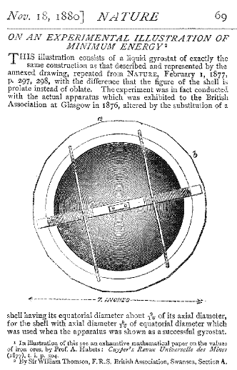
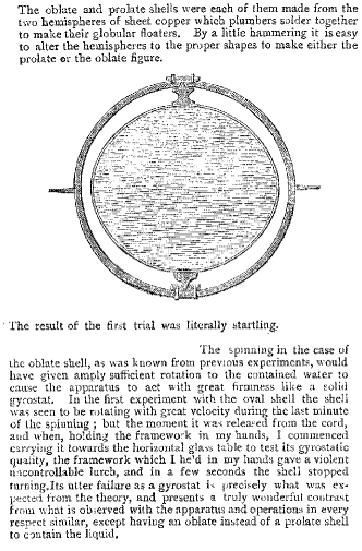
Figure 1: The Kelvin gyrostat WT1880 .

Already von Laue (1905) VL1905 , Lamb (1908) Lamb1908 and Heisenberg (1924) H1924 realized that dissipation easily destabilizes waves and modes of negative energy of an ideal system supported by rotating and translating continua S1958 ; S1960 . Williamson (1936) proposed normal forms for Hamiltonian systems allowing sorting stable modes of negative and positive energy according to their symplectic sign MK86 ; W1936 ; W1937 . However, further generalization — the theory of spaces with indefinite metric, or Krein K1983 and Pontryagin P44 spaces, — was directly inspired by the problem of stability of the Kelvin gyrostat G1880 ; WT1880 , having both astrophysical and industrial (and even military) applications.

Kelvin WT1880 experimentally demonstrated in 1880 that a thin-walled and slightly oblate spheroid completely filled with liquid remains stable if rotated fast enough about a fixed point, which does not happen if the spheroid is slightly prolate, Figure 1. In the same year this observation was confirmed theoretically by Greenhill G1880 , who found that rotation around the center of gravity of the top in the form of a weightless ellipsoidal shell completely filled with an ideal and incompressible fluid, is unstable when $a<c<3a$, where $c$ is the length of the semiaxis of the ellipsoid along the axis of rotation and the lengths of the two other semiaxes are equal to $a$ G1880 .

Quite similarly, bullets and projectiles fired from the rifled weapons can relatively easily be stabilized by rotation, if they are solid inside. In contrast, the shells, containing a liquid substance inside, have a tendency to turn over despite seemingly revolved fast enough to be gyroscopically stabilized. Motivated by such artillery applications, in 1942 Sobolev, then director of the Steklov Mathematical Institute in Moscow, considered stability of a rotating heavy top with a cavity entirely filled with an ideal incompressible fluid S2006 —a problem that is directly connected to the classical XIXth century models of astronomical bodies with a crust surrounding a molten core S1959 .

For simplicity, the solid shell of the top and the domain $V$ occupied by the cavity inside it, can be assumed to have a shape of a solid of revolution. They have a common symmetry axis where the fixed point of the top is located. The velocity profile of the stationary unperturbed motion of the fluid is that of a solid body rotating with the same angular velocity $\Omega$ as the shell around the symmetry axis.

Following Sobolev, we denote by $M_{1}$ the mass of the shell, $M_{2}$ the mass of the fluid, $\rho$ and $p$ the density and the pressure of the fluid, $g$ the gravity acceleration, and $l_{1}$ and $l_{2}$ the distances from the fixed point to the centers of mass of the shell and the fluid, respectively. The moments of inertia of the shell and the ‘frozen’ fluid with respect to the symmetry axis are $C_{1}$ and $C_{2}$, respectively; $A_{1}$ ($A_{2}$) stands for the moment of inertia of the shell (fluid) with respect to any axis that is orthogonal to the symmetry axis and passes through the fixed point. Let, additionally,

$$L=C_{1}+C_{2}-A_{1}-A_{2}-\frac{K}{\Omega^{2}},\quad K=g(l_{1}M_{1}+l_{2}M_{2}).$$ (1)

The solenoidal $(\textrm{div}\,\textbf{v}=0)$ velocity field v of the fluid is assumed to satisfy the no-flow condition on the boundary of the cavity: $\left.\textbf{ v}_{n}\right|_{\partial V}=0$.

Stability of the stationary rotation of the top around its vertically oriented symmetry axis is determined by the system of linear equations derived by Sobolev in the frame $(x,y,z)$ that has its origin at the fixed point of the top and rotates with respect to an inertial frame around the vertical $z$-axis with the angular velocity of the unperturbed top, $\Omega$. If the real and imaginary part of the complex number $Z$ describe the deviation of the unit vector of the symmetry axis of the top in the coordinates $x$, $y$, and $z$, then these equations are, see e.g. S2006 ; Y97 :

$$\frac{dZ}{dt} = i\Omega W,$$

$$(A_{1}{+}\rho\kappa^{2})\frac{dW}{dt} = i\Omega LZ+i\Omega(C_{1}{-}2A_{1}{+}\rho E)W+i\rho\int_{V}\left(v_{x}\frac{\partial\chi}{\partial y}-v_{y}\frac{\partial\chi}{\partial x}\right)dV,$$

$$\partial_{t}v_{x} = 2\Omega v_{y}-{\rho}^{-1}\partial_{x}p+2i\Omega^{2}W\partial_{y}\overline{\chi},$$

$$\partial_{t}v_{y} = -2\Omega v_{x}-{\rho}^{-1}\partial_{y}p-2i\Omega^{2}W\partial_{x}\overline{\chi},$$

$$\partial_{t}v_{z} = -{\rho}^{-1}\partial_{z}p,$$ (2)

where $2\kappa^{2}=\int_{V}|\nabla\chi|^{2}dV$, $E=i\int_{V}\left(\partial_{x}\overline{\chi}\partial_{y}\chi-\partial_{y}\overline{\chi}\partial_{x}\chi\right)dV$, and the function $\chi$ is determined by the conditions

$$\nabla^{2}\chi=0,\quad\left.\partial_{n}\chi\right|_{\partial V}=z(\cos nx+i\cos ny)-(x+iy)\cos nz,$$ (3)

with $n$ the absolute value of a vector n, normal to the boundary of the cavity.

Sobolev realized that some qualitative conclusions on the stability of the top can be drawn with the use of the bilinear form

$$Q(R_{1},R_{2})=L\Omega Z_{1}\overline{Z}_{2}+(A_{1}+\rho\kappa^{2})W_{1}\overline{W}_{2}+\frac{\rho}{2\Omega^{2}}\int_{V}\overline{\textbf{v}}_{2}^{T}\textbf{v}_{1}dV$$ (4)

on the elements $R_{1}$ and $R_{2}$ of the space $\{R\}=\{Z,W,\textbf{v}\}$. The linear operator $B$ defined by Eqs. (1.1) that can be written as $\frac{dR}{dt}=iBR$ has all its eigenvalues real when $L>0$, which yields Lyapunov stability of the top. The number of pairs of complex-conjugate eigenvalues of $B$ (counting multiplicities) does not exceed the number of negative squares of the quadratic form $Q(R,R)$, which can be equal only to one when $L<0$. Hence, for $L<0$ an unstable solution $R=e^{i\lambda_{0}t}R_{0}$ can exist with $\textrm{ Im}\lambda_{0}<0$; all real eigenvalues are simple except for maybe one S2006 ; Y97 ; Kopachevskii2001 .

In the particular case when the cavity is an ellipsoid of rotation with the semi-axes $a$, $a$, and $c$, the space of the velocity fields of the fluid can be decomposed into a direct sum of subspaces, one of which is finite-dimensional. Only the movements from this subspace interact with the movements of the rigid shell, which yields a finite-dimensional system of ordinary differential equations that describes coupling between the shell and the fluid.

Calculating the moments of inertia of the fluid in the ellipsoidal container

$$C_{2}=\frac{8\pi\rho}{15}a^{4}c,\quad A_{2}=l_{2}^{2}M_{2}+\frac{4\pi\rho}{15}a^{2}c(a^{2}+c^{2}),$$

denoting $m=\frac{c^{2}-a^{2}}{c^{2}+a^{2}}$, and assuming the field $\textbf{ v}=(v_{x},v_{y},v_{z})^{T}$ in the form

$$v_{x}=(z-l_{2})a^{2}m\xi,\quad v_{y}=-i(z-l_{2})a^{2}m\xi,\quad v_{z}=-(x-iy)c^{2}m\xi,$$

one can eliminate the pressure in Eqs. (1.1) and obtain the reduced model

$$\frac{d\textbf{x}}{dt}=i\Omega\textbf{A}^{-1}\textbf{C}\textbf{x}=i\Omega\textbf{B}\textbf{x},$$ (5)

where $\textbf{x}=(Z,W,\xi)^{T}\in\mathbb{C}^{3}$ and

A $$= \left(\begin{array}[]{ccc}1&0&0\\ 0&A_{1}{+}l_{2}^{2}M_{2}{+}\frac{4\pi\rho}{15}a^{2}c\frac{(c^{2}-a^{2})^{2}}{c^{2}+a^{2}}&0\\ 0&0&c^{2}+a^{2}\\ \end{array}\right),$$ (9)

C $$= \left(\begin{array}[]{ccc}0&1&0\\ L&C_{1}{-}2A_{1}{-}2l_{2}^{2}M_{2}{-}\frac{8\pi\rho}{15}a^{2}c^{3}m^{2}&-\frac{8\pi\rho}{15}a^{4}c^{3}m^{2}\\ 0&-2&-2a^{2}\\ \end{array}\right).$$ (13)

The matrix $\textbf{B}\neq\textbf{B}^{T}$ in Eq. (5) after multiplication by a symmetric matrix

$$\textbf{G}=\left(\begin{array}[]{ccc}L&0&0\\ 0&A_{1}{+}l_{2}^{2}M_{2}{+}\frac{4\pi\rho}{15}a^{2}c\frac{(c^{2}-a^{2})^{2}}{c^{2}+a^{2}}&0\\ 0&0&\frac{4\pi\rho}{15}a^{4}c^{3}\frac{(c^{2}-a^{2})^{2}}{c^{2}+a^{2}}\\ \end{array}\right)$$ (14)

yields a Hermitian matrix $\textbf{G}\textbf{B}=\overline{(\textbf{G}\textbf{B})}^{T}$, i.e. B is a self-adjoint operator in the space $\mathbb{C}^{3}$ endowed with the metric

$$[\textbf{u},\textbf{u}]:=(\textbf{G}\textbf{u},\textbf{u})=\overline{\textbf{u}}^{T}\textbf{G}\textbf{u},\quad\textbf{u}\in\mathbb{C}^{3},$$ (15)

which is definite when $L>0$ and indefinite with one negative square when $L<0$. If $\lambda$ is an eigenvalue of the matrix B, i.e. $\textbf{B}\textbf{u}=\lambda\textbf{u}$, then $\overline{\textbf{u}}^{T}\textbf{G}\textbf{B}\textbf{u}=\lambda\overline{\textbf{u}}^{T}\textbf{G}\textbf{u}$. On the other hand, $\overline{\textbf{u}}^{T}(\overline{\textbf{G}\textbf{B}})^{T}\textbf{u}=\overline{\lambda}\,\overline{\overline{\textbf{u}}^{T}\textbf{G}\textbf{u}}=\overline{\lambda}\,{\overline{\textbf{u}}^{T}\textbf{G}\textbf{u}}$. Hence,

$$(\lambda-\overline{\lambda})\overline{\textbf{u}}^{T}\textbf{G}\textbf{u}=0,$$

implying $\overline{\textbf{u}}^{T}\textbf{G}\textbf{u}=0$ on the eigenvector u of the complex $\lambda\neq\overline{\lambda}$. For real eigenvalues $\lambda=\overline{\lambda}$ and $\overline{\textbf{u}}^{T}\textbf{G}\textbf{u}\neq 0$. The sign of the quantity $\overline{\textbf{u}}^{T}\textbf{G}\textbf{u}$ (or Krein sign) can be different for different real eigenvalues.

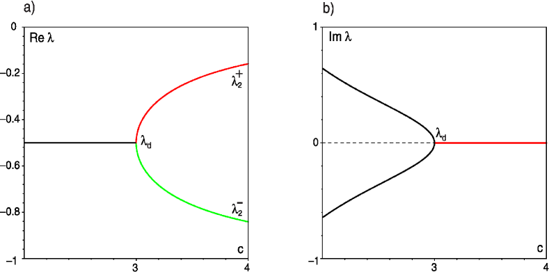
Figure 2: (a) Simple real eigenvalues (16) of the Sobolev’s top in the Greenhill’s case for $a=1$ with (red) $\overline{\textbf{u}}^{T}\textbf{G}\textbf{u}>0$ and (green) $\overline{\textbf{u}}^{T}\textbf{G}\textbf{u}<0$. (b) At simple complex-conjugate eigenvalues (black) and at the double real eigenvalue $\lambda_{d}$ we have $\overline{\textbf{u}}^{T}\textbf{G}\textbf{u}=0$.

For example, when the ellipsoidal shell is massless and the supporting point is at the center of mass of the system, then $A_{1}=0$, $C_{1}=0$, $M_{1}=0$, $l_{2}=0$. The matrix B has thus one real eigenvalue $(\lambda_{1}^{+}=-1,~{}{\overline{\textbf{u}}_{1}^{+}}^{T}\textbf{G}\textbf{u}_{1}^{+}>0)$ and the pair of eigenvalues

$$\lambda_{2}^{\pm}=-\frac{1}{2}\pm\frac{1}{2}\sqrt{1+\frac{32\pi\rho}{15}\frac{ca^{4}}{L}},\quad L=\frac{4\pi\rho}{15}a^{2}c(a^{2}-c^{2}),$$ (16)

which are real if $L>0$ and can be complex if $L<0$. The latter condition together with the requirement that the radicand in Eq. (16) is negative, reproduces the Greenhill’s instability zone: $a<c<3a$ G1880 . With the change of $c$, the real eigenvalue $\lambda_{2}^{+}$ with ${\overline{\textbf{u}}_{2}^{+}}^{T}\textbf{G}\textbf{u}_{2}^{+}>0$ collides at $c=3a$ with the real eigenvalue $\lambda_{2}^{-}$ with ${\overline{\textbf{u}}_{2}^{-}}^{T}\textbf{G}\textbf{u}_{2}^{-}<0$ into a real double defective eigenvalue $\lambda_{d}$ with the algebraic multiplicity two and geometric multiplicity one. This Krein collision is illustrated in Figure 2. Note that ${\overline{\textbf{u}}_{d}}^{T}\textbf{G}\textbf{u}_{d}=0$, where $\textbf{u}_{d}$ is the eigenvector at $\lambda_{d}$.

Therefore, in the case of the ellipsoidal shapes of the shell and the cavity, the Hilbert space $\{R\}=\{Z,W,\textbf{v}\}$ of the Sobolev’s problem endowed with the indefinite metric $(L<0)$ decomposes into the three-dimensional space of the reduced model (5), where the self-adjoint operator $B$ can have complex eigenvalues and real defective eigenvalues, and a complementary infinite-dimensional space, which is free of these complications. The very idea that the signature of the indefinite metric can serve for counting unstable eigenvalues of an operator that is self-adjoint in a functional space equipped with such a metric, turned out to be a concept of a rather universal character possessing powerful generalizations that were initiated by Pontryagin in 1944 P44 and developed into a general theory of indefinite inner product spaces or Krein spaces Bognar1974 ; KM2014 ; K1983 . Relation of the Krein sign to the sign of energy or action has made it a popular tool for predicting instabilities in physics N1976 ; Z2016 .

1.2 Secular instability of the Maclaurin spheroids by viscous and radiative losses

It is hard to find a physical application that would stimulate development of mathematics to such an extent as the problem of stability of equilibria of rotating and self-gravitating masses of fluids. Rooted in the Newton and Cassini thoughts on the actual shape of the Earth, the rigorous analysis of this question attracted the best minds of the XVIII-th and XIX-th centuries, from Maclaurin to Riemann, Poincaré and Lyapunov. In fact, modern nonlinear dynamics AA88 ; IA92 ; Kuz04 and Lyapunov stability theory L1992 are by-products of the efforts invested in solution of this question of the astrophysical fluid dynamics BKM2009 , which experiences a revival nowadays A2003 inspired by the recent detection of gravitational waves Abb17 .

We recall that in 1742 Maclaurin established that an oblate spheroid

$$\frac{x^{2}}{a_{1}^{2}}+\frac{y^{2}}{a_{2}^{2}}+\frac{z^{2}}{a_{3}^{2}}=1,\quad a_{3}<a_{2}=a_{1}$$

is a shape of relative equilibrium of a self-gravitating mass of inviscid fluid in a solid-body rotation about the $z$-axis, provided that the rate of rotation, $\Omega$, is related to the eccentricity $e=\sqrt{1-\frac{a_{3}^{2}}{a_{1}^{2}}}$ through the formula M1742

$$\Omega^{2}(e)=2e^{-3}(3-2e^{2})\sin^{-1}(e)\sqrt{1-e^{2}}-6e^{-2}(1-e^{2}).$$ (17)

A century later, Jacobi (1834) has discovered less symmetric shapes of relative equilibria in this problem that are tri-axial ellipsoids

$$\frac{x^{2}}{a_{1}^{2}}+\frac{y^{2}}{a_{2}^{2}}+\frac{z^{2}}{a_{3}^{2}}=1,\quad a_{3}<a_{2}<a_{1}.$$

Later on a student of Jacobi, Meyer (1842) M1842 , and then Liouville (1851) L1851 have shown that the family of Jacobi’s ellipsoids has one member in common with the family of Maclaurin’s spheroids at $e\approx 0.8127$. The equilibrium with the Meyer-Liouville eccentricity is neutrally stable.

In 1860 Riemann R1860 established neutral stability of inviscid Maclaurin’s spheroids on the interval of eccentricities $(0<e<0.952..)$. At the Riemann point with the critical eccentricity $e\approx 0.9529$ the Hamilton-Hopf bifurcation sets in and causes dynamical instability with respect to ellipsoidal perturbations beyond this point DS1979 ; S1980-2 ; S1980-3 .

A century later Chandrasekhar C1969 used a virial theorem to reduce the problem to a finite-dimensional system, which stability is governed by the eigenvalues of the matrix polynomial

$${\mathbf{L}}_{i}(\lambda)=\lambda^{2}\left(\begin{array}[]{cc}1&0\\ 0&1\\ \end{array}\right)+\lambda\left(\begin{array}[]{cc}0&-4\Omega\\ \Omega&0\\ \end{array}\right)+\left(\begin{array}[]{cc}4b-2\Omega^{2}&0\\ 0&4b-2\Omega^{2}\\ \end{array}\right),$$ (18)

where $\Omega(e)$ is given by the Maclaurin law (17) and $b(e)$ is as follows

$$b=\frac{\sqrt{1-e^{2}}}{4e^{5}}\left\{e(3-2e^{2})\sqrt{1-e^{2}}+(4e^{2}-3)\sin^{-1}(e)\right\}.$$ (19)

The eigenvalues of the matrix polynomial (18) are

$$\lambda=\pm\left(i\Omega\pm i\sqrt{4b-\Omega^{2}}\right).$$ (20)

Requiring $\lambda=0$ we can determine the critical Meyer-Liouville eccentricity by solving with respect to $e$ the equation C1969

$$4b(e)=2\Omega^{2}(e).$$

The critical eccentricity at the Riemann point follows from requiring the radicand in (20) to vanish:

$$4b(e)=\Omega^{2}(e),$$

which is equivalent to the equation

$$e=\sin\left(\frac{e(3+4e^{2})\sqrt{1-e^{2}}}{3+2e^{2}-4e^{4}}\right)$$

that has a root $e\approx 0.9529$.

Remarkably, when

$$\Omega^{2}(e)<4b(e)<2\Omega^{2}(e)$$ (21)

both eigenvalues of the stiffness matrix

$$\left(\begin{array}[]{cc}4b-2\Omega^{2}&0\\ 0&4b-2\Omega^{2}\\ \end{array}\right)$$

are negative. The number of negative eigenvalues of the matrix of potential forces is known as the Poincaré instability degree. The Poincaré instability degree of the equilibria with the eccentricities (21) is even and equal to 2. Hence, the interval (21) corresponding to $0.812..<e<0.952..$, which is stable according to Riemann, is, in fact, the interval of gyroscopic stabilization L2013 of the Maclaurin spheroids, Figure 3.

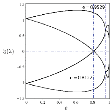
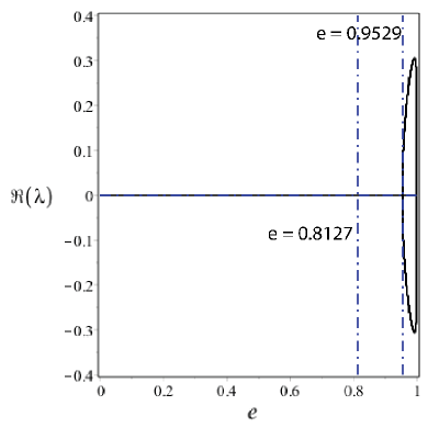
Figure 3: (Left) Frequencies and (right) growth rates of the eigenvalues of the inviscid eigenvalue problem $\textbf{L}_{i}(\lambda)\textbf{u}=0$ demonstrating the Hamilton-Hopf bifurcation at the Riemann critical value of the eccentricity, $e\approx 0.9529$ and neutral stability at the Meyer-Liouville point, $e\approx 0.8127$.

In 1879 Kelvin and Tait TT realized that viscosity of the fluid can destroy the gyroscopic stabilization of the Maclaurin spheroids: “If there be any viscosity, however slight, in the liquid, the equilibrium [beyond $e\approx 0.8127$] in any case of energy either a minimax or a maximum cannot be secularly stable”.

The prediction made by Kelvin and Tait TT has been rigorously verified only in the XX-th century by Roberts and Stewartson RS1963 . Using the virial approach by Chandrasekhar, the linear stability problem can be reduced to the study of eigenvalues of the matrix polynomial

$${\mathbf{L}}_{v}(\lambda)=\lambda^{2}\left(\begin{array}[]{cc}1&0\\ 0&1\\ \end{array}\right)+\lambda\left(\begin{array}[]{cc}10\mu&-4\Omega\\ \Omega&10\mu\\ \end{array}\right)+\left(\begin{array}[]{cc}4b-2\Omega^{2}&0\\ 0&4b-2\Omega^{2}\\ \end{array}\right),$$ (22)

where $\mu=\frac{\nu}{a_{1}^{2}\sqrt{\pi G\rho}}$, $\nu$ is the viscosity of the fluid, $G$ is the universal gravitation constant, and $\rho$ the density of the fluid C1969 . The $\lambda$ and $\Omega$ are measured in units of $\sqrt{\pi G\rho}$. The operator ${\mathbf{L}}_{v}(\lambda)$ differs from the operator of the ideal system, ${\mathbf{L}}_{i}(\lambda)$, by the matrix of dissipative forces $10\lambda\mu\textbf{I}$, where I is the $2\times 2$ unit matrix.

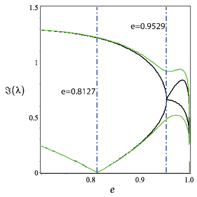
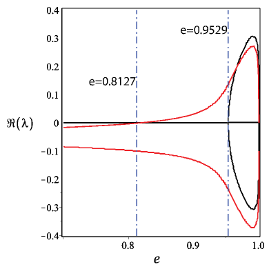
Figure 4: (Left) Frequencies and (right) growth rates of the (black lines) inviscid Maclaurin spheroids and (green and red lines) viscous ones with $\mu=\frac{\nu}{a_{1}^{2}\sqrt{\pi G\rho}}=0.01$. Viscosity destroys the gyroscopic stabilization of the Maclaurin spheroids on the interval $0.8127..<e<0.9529..$, which is stable in the inviscid case C1969 ; C1984 ; RS1963 .

The characteristic polynomial written for ${\mathbf{L}}_{v}(\lambda)$ yields the equation governing the growth rates of the ellipsoidal perturbations in the presence of viscosity:

$$25\Omega^{2}\mu^{2}+({\mathrm{R}e}\lambda+5\mu)^{2}(\Omega^{2}-{\mathrm{R}e}\lambda^{2}-10{\mathrm{R}e}\lambda\mu-4b)=0.$$ (23)

The right panel of Figure 4 shows that the growth rates (23) become positive beyond the Meyer-Liouville point. Indeed, assuming ${\mathrm{R}e}\lambda=0$ in (23), we reduce it to $50\mu^{2}(\Omega^{2}-2b)=0,$ meaning that the growth rate vanishes when $\Omega^{2}=2b$ no matter how small the viscosity coefficient $\mu$ is. But, as we already know, the equation $\Omega^{2}(e)=2b(e)$ determines exactly the Meyer-Liouville point, $e\approx 0.8127$.

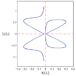
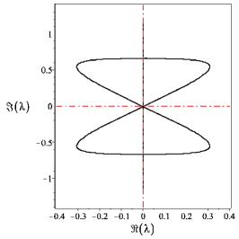
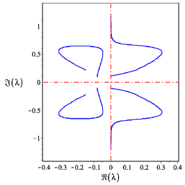
Figure 5: Paths of the eigenvalues in the complex plane for (left) viscous Maclaurin spheroids with $\mu=\frac{\nu}{a_{1}^{2}\sqrt{\pi G\rho}}=0.002$, (centre) Maclaurin spheroids without dissipation, and (right) inviscid Maclaurin spheroids with radiative losses for $\delta=0.05$. The collision of two modes of the non-dissipative Hamiltonian system shown in the centre occurs at the Riemann critical value $e\approx 0.9529$. Both types of dissipation destroy the collision and destabilize one of the two interacting modes at the Meyer-Liouville critical value $e\approx 0.8127$.

It turns out, that the critical eccentricity of the viscous Maclaurin spheroid is equal to the Meyer-Liouville value, $e\approx 0.8127$, even in the limit of vanishing viscosity, $\mu\rightarrow 0$, and thus does not converge to the inviscid Riemann value $e\approx 0.9529$.

Viscous dissipation destroys the interaction of two modes at the Riemann critical point and destabilizes one of them beyond the Meyer-Liouville point, showing an avoided crossing in the complex plane, Figure 5(left).

Kelvin and Tait TT hypothesised that the instability, which is stimulated by the presence of viscosity in the fluid, will result in a slow, or secular, departure of the system from the unperturbed equilibrium of the Maclaurin family at the Meyer-Liouville point and subsequent evolution along the Jacobi family, as long as the latter is stable C1969 .

Therefore, a rotating, self-gravitating fluid mass, initially symmetric about the axis of rotation, can undergo an axisymmetric evolution in which it first loses stability to a nonaxisymmetric disturbance, and continues evolving along a non-axisymmetric family toward greater departure from axial symmetry; then it undergoes a further loss of stability to a disturbance tending toward splitting into two parts. Rigorous mathematical treatment of the validity of the fission theory of binary stars by Lyapunov and Poincaré has laid a foundation to modern nonlinear analysis. In particular, it has led Lyapunov to the formulation of a general theory of stability of motion BKM2009 .

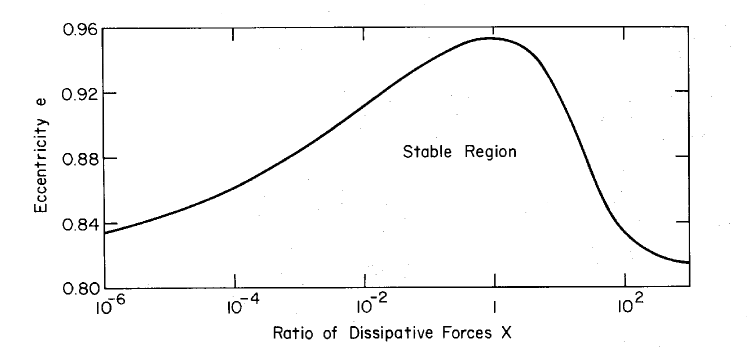
Figure 6: Critical eccentricity in the limit of vanishing dissipation depends on the damping ratio, $X$, and attains its maximum (Riemann) value, $e\approx 0.9529$ exactly at $X=1$. As $X$ tends to zero or infinity, the critical value tends to the Meyer-Liouville value $e\approx 0.8127$, LD1977 ; C1984 .

In 1970 Chandrasekhar C1970 demonstrated that there exists another mechanism making Maclaurin spheroids unstable beyond the Meyer-Liouville point of bifurcation, namely, the radiative losses due to emission of gravitational waves. However, the mode that is made unstable by the radiation reaction is not the same one that is made unstable by the viscosity, Figure 5(right).

In the case of the radiative damping mechanism stability is determined by the spectrum of the following matrix polynomial C1970

$$\textbf{L}_{g}(\lambda)=\lambda^{2}+\lambda(\textbf{G}+\textbf{D})+\textbf{K}+\textbf{N}$$

that contains the matrices of gyroscopic, G, damping, D, potential, K, and nonconservative positional, N, forces

$$\textbf{G}=\frac{5}{2}\left(\begin{array}[]{rr}0&-\Omega\\ \Omega&0\\ \end{array}\right),\quad\textbf{D}=\left(\begin{array}[]{cc}\delta 16\Omega^{2}(6b-\Omega^{2})&-3\Omega/2\\ -3\Omega/2&\delta 16\Omega^{2}(6b-\Omega^{2})\\ \end{array}\right)$$

$$\textbf{K}=\left(\begin{array}[]{cc}4b-\Omega^{2}&0\\ 0&4b-\Omega^{2}\\ \end{array}\right),\quad\textbf{N}=\delta\left(\begin{array}[]{cc}2q_{1}&2q_{2}\\ -q_{2}/2&2q_{1}\\ \end{array}\right),$$

where $\Omega(e)$ and $b(e)$ are given by equations (17) and (19). Explicit expressions for $q_{1}$ and $q_{2}$ can be found in C1970 . The coefficient $\delta=\frac{GMa_{1}^{2}(\pi G\rho)^{3/2}}{5c^{5}}$ is related to gravitational radiation reaction, $G$ is the universal gravitation constant, $\rho$ the density of the fluid, $M$ the mass of the ellipsoid, and $c$ the velocity of light in vacuum.

In 1977 Lindblom and Detweiler LD1977 studied the combined effects of the gravitational radiation reaction and viscosity on the stability of the Maclaurin spheroids. As we know, each of these dissipative effects induces a secular instability in the Maclaurin sequence past the Meyer-Liouville point of bifurcation. However, when both effects are considered together, the sequence of stable Maclaurin spheroids reaches past the bifurcation point to a new point determined by the ratio, $X=\frac{25}{2\Omega_{0}^{4}}\frac{\mu}{\delta}$, of the strengths of the viscous and radiation reaction forces, where $\Omega_{0}=0.663490...$.

Figure 6 shows the critical eccentricity as a function of the damping ratio in the limit of vanishing dissipation. This limit coincides with the inviscid Riemann point only at a particular damping ratio. At any other ratio, the critical value is below the Riemann one and tends to the Meyer-Liouville value as this ratio tends either to zero or infinity. Lindblom and Detweiler LD1977 correctly attributed the cancellation of the secular instabilities to the fact that viscous dissipation and radiation reaction cause different modes to become unstable, see Figure 5. In fact, the mode destabilized by the fluid viscosity is the prograde moving spherical harmonic that appears to be retrograde in the frame rotating with the fluid mass and the mode destabilized by the radiative losses is the retrograde moving spherical harmonic when it appears to be prograde in the inertial frame A2003 . It is known Lamb1908 ; N1976 that to excite the positive energy mode one must provide additional energy to the mode, while to excite the negative energy mode one must extract energy from the mode C95 ; Sa08 . The latter can be done by dissipation and the former by the non-conservative positional forces K07b ; K09 ; K2013dg . Both are present in the model by Lindblom and Detweiler LD1977 .

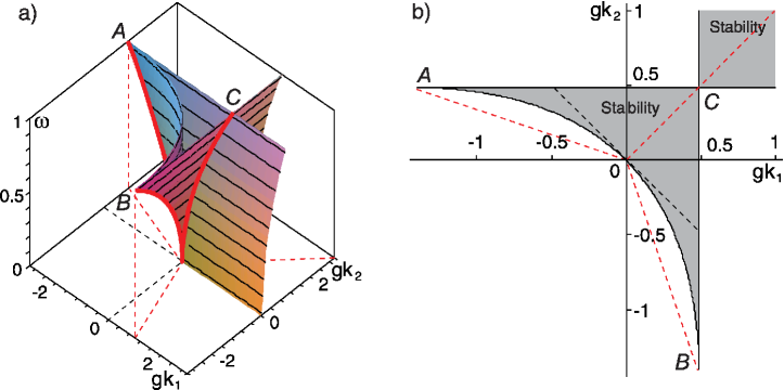
Figure 7: (a) Stability domain (25) of the Brouwer’s rotating vessel and (b) its cross-section at $\omega=0.7$ K2011b ; K2013dg .

1.3 Brouwer’s rotating vessel

In 1918, Brouwer B18 published a simple model for the motion of a point mass near the bottom of a rotating vessel. For an English translation see B76 pp. 665-675. The shape of the vessel is described by a surface $S$, rotating around a vertical axis with constant angular velocity $\omega$. With the equilibrium chosen on the vertical axis at $(x,y)=(0,0)$ on $S$, the linearized equations of motion without dissipation are

$$\ddot{x}-2\omega\dot{y}+(gk_{1}-\omega^{2})x = 0,$$

$$\ddot{y}+2\omega\dot{x}+(gk_{2}-\omega^{2})y = 0.$$ (24)

The constants $k_{1}$ and $k_{2}$ are the $x,y$-curvatures of $S$ at $(0,0)$, $g$ is the gravitational constant. Suppose that $k_{1}\geq k_{2}$.

Stability and instability without friction
Assuming there is no damping, there are the following three cases:

• $0<k_{2}<k_{1}$ (single-well at equilibrium).
  Stability iff $0<\omega^{2}<gk_{2}$ (slow rotation) or $\omega^{2}>gk_{1}$ (fast rotation).

• $k_{2}<0$ and $k_{1}>0,\,k_{1}>-k_{2}$ (saddle at equilibrium).
  Stability iff $\omega^{2}>gk_{1}$.

• $k_{2}<0$ and $k_{1}>0,\,k_{1}<-k_{2}$ (saddle).
  If $3k_{1}+k_{2}<0$: instability.
  If $3k_{1}+k_{2}>0$: stability if

  $$gk_{1}<\omega^{2}<-\frac{g}{8}\frac{(k_{1}-k_{2})^{2}}{(k_{1}+k_{2})}.$$ (25)

• $k_{1}<0,\,k_{2}<0$: instability.

Stability of triangular libration points $L_{4}$ and $L_{5}$
Brouwer’s rotating vessel model includes both a well with two positive curvatures $k_{1}$ and $k_{2}$ and a saddle with the curvatures of opposite signs. Remarkably, the latter case describes stability of triangular libration points $L_{4}$ and $L_{5}$ (discovered by Lagrange in 1772) in the restricted circular three-body problem of celestial mechanics. Indeed, the linearized equation for this problem is (1.3) where $\omega=1$,

$$gk_{1} = -\frac{1}{2}+\frac{3}{2}\sqrt{1-3\mu(1-\mu)}\geq\frac{1}{4},$$

$$gk_{2} = -\frac{1}{2}-\frac{3}{2}\sqrt{1-3\mu(1-\mu)}\leq-\frac{5}{4},$$ (26)

$\mu=\frac{m_{1}}{m_{1}+m_{2}}$, and $m_{1}$ and $m_{2}$ are the masses of the two most massive bodies (in comparison with each of them the mass of the third body is assumed to be negligible) A1970 ; G1843 ; R2002 . Since $k_{1}$ and $k_{2}$ are of opposite signs for all $0\leq\mu\leq 1$, the linear stability of the triangular Lagrange equilibriums is determined by the stability conditions (25) for the rotating saddle BB1994 . Note that the coefficients (1.3) satisfy the constraint $gk_{1}+gk_{2}=-1$. Intervals of intersection of this line with the narrow corners of the curvilinear triangle in Figure 7b correspond to the stable Lagrange points. After substitution of (1.3) into (7), we reproduce the classical condition for their linear stability first established by Gascheau in 1843 G1843

$$(gk_{1}-gk_{2})^{2}-8=1-27\mu(1-\mu)>0.$$

Stability in a rotating saddle potential is a subject of current active discussion in respect with the particle trapping BB1994 ; BC2018 ; K2011b ; JMT2017 . An effect of slow precession of trajectories of the trapped particles in a rotating saddle potential KL2017 ; S1998 has recently inspired new works leading to the improvement of traditional averaging methods CL2018 ; YH2018 .

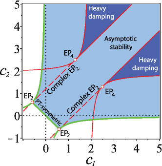
Figure 8: Domain of asymptotic stability of the damped Brouwer’s rotating vessel in the plane of the damping coefficients for $gk_{1}=1$, $gk_{2}=1$, and $\omega=0.3$ K2013dg ; K2013pt .

Destabilization by friction
Adding constant (Coulomb) damping, Brouwer B18 finds a number of instability cases. The equations of motion become in this case:

$$\ddot{x}-2\omega\dot{y}+c_{1}\dot{x}+(gk_{1}-\omega^{2})x = 0,$$ (27)

$$\ddot{y}+2\omega\dot{x}+c_{2}\dot{y}+(gk_{2}-\omega^{2})y = 0.$$ (28)

The friction constants $c_{1},c_{2}$ are positive. The characteristic (eigenvalue) equation takes the form:

$$\lambda^{4}+a_{1}\lambda^{3}+a_{2}\lambda^{2}+a_{3}\lambda+a_{4}=0,$$

with $a_{1}=c_{1}+c_{2}$,
$a_{2}=g(k_{1}+k_{2})+2\omega^{2}+c_{1}c_{2}$
$a_{3}=c_{1}(gk_{2}-\omega^{2})+c_{2}(gk_{1}-\omega^{2})$,
$a_{4}=(gk_{1}-\omega^{2})(gk_{2}-\omega^{2})$.

There are two cases that drastically change the stability (see also Bottema Bo76 ) :

• $0<k_{2}<k_{1}$ (single-well).
  Stability iff $0<\omega^{2}<gk_{2}$.
  The fast rotation branch $\omega^{2}>gk_{1}$ has vanished.

• $k_{2}<0$ and $k_{1}>0,\,k_{1}<-k_{2}$ (saddle).
  The requirement $a_{4}>0$ produces $0<gk_{1}<\omega\texttwosuperior$. This is not compatible with $a_{3}<0$ so a saddle is always unstable with any size of positive damping.

Brouwer studied this model probably to use in his lectures. In a correspondence with O. Blumenthal and G. Hamel he asked whether the results of the calculations were known; see B76 pp. 677-686. Hamel confirmed that the results were correct and surprising, but there is no reference to older literature in this correspondence. See also Bo76 .

Indefinite damping and PT-symmetry
Brouwer’s model for the case of a rotating well with two positive curvatures has a direct relation to rotordynamics as it contains the Jeffcott rotor model, see for instance K2011b . Dissipation induces instabilities in this model at high speeds of rotation $\omega$ Bo63 ; C95 ; S33 , of course, under the assumption that the damping coefficients are both positive. But what happens if we relax this constraint and extend the space of damping parameters to negative values? It turns out that at low speeds $\omega$ the domain of asymptotic stability spreads to the area of negative damping, Figure 8. Even more, a part of the neutral stability curve belongs to the line $c_{1}+c_{2}=0$ where one of the damping coefficients is positive and the other one is negative. On this line the system is invariant under time and parity reversion transformation and is therefore $PT$-symmetric. Its eigenvalues are imaginary in spite of the presence of the loss (positive damping) and gain (negative damping) in the system. $PT$-symmetric systems with the indefinite damping can easily be realized in the laboratory experiments Kottos2011 . Recent study Z2018 shows their connection to complex G-Hamiltonian systems KI2017 ; YS75 .

2 Ziegler’s paradox

We already know that Greenhill’s analysis of stability of the Kelvin gyrostat G1880 inspired the works of Sobolev S2006 and Pontryagin P44 which have led to the development of the theory of spaces with indefinite inner product Bognar1974 ; K1983 . Another work of Greenhill G1883 ultimately brought about the famous Ziegler paradox Z52 . As Gladwell remarked in his historical account of the genesis of the field of nonconservative stability G1990 , “It was Greenhill who started the trouble though he never knew it.”

Motivated by the problem of buckling of propeller-shafts of steamers Greenhill (1883) analyzed stability of an elastic shaft of a circular cross-section under the action of a compressive force and an axial torque G1883 . He managed to find the critical torque that causes buckling of the shaft for a number of boundary conditions. For the clamped-free and the clamped-hinged shaft loaded by an axial torque the question remained open until Nicolai in 1928 reconsidered a variant of the clamped-hinged boundary conditions, in which the axial torque is replaced with the follower torque N1928 . The vector of the latter is directed along the tangent to the deformed axis of the shaft at the end point G1990 .

Nicolai had established that no nontrivial equilibrium configuration of the shaft exists different from the rectilinear one, meaning stability for all magnitudes of the follower torque. Being unsatisfied with this overoptimistic result, he assumed that the equilibrium method does not work properly in the case of the follower torque. He decided to study small oscillations of the shaft about its rectilinear configuration using what is now known as the Lyapunov stability theory L1992 that, in particular, can predict instability via eigenvalues of the linearized problem.

Surprisingly, it turned out that there exist eigenvalues with positive real parts (instability) for all magnitudes of the torque, meaning that the critical value of the follower torque for an elastic shaft of a circular cross-section is actually zero. Because of its unusual behavior, this instability phenomenon received a name “Nicolai’s paradox” G1990 ; LFA2016 ; N1928 .

In 1951-56 Hans Ziegler of the ETH Zürich re-considered the five original Greenhill problems with the Lyapunov approach and found that the shaft is unstable in cases of the clamped-free and the clamped-hinged boundary conditions for all values of the axial torque, just as in Nicolai’s problem with the follower torque Z53 . Moreover, the non-self-adjoint boundary eigenvalue problem for the Greenhill’s shaft with the axial torque turned out to be a Hermitian adjoint of the non-self-adjoint boundary eigenvalue problem for the Greenhill’s shaft with the follower torque Bo63 .

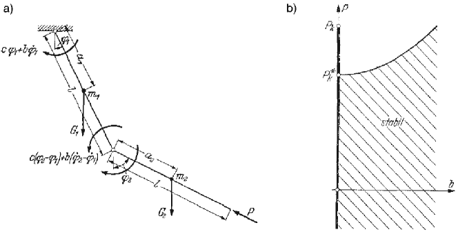
Figure 9: Original drawings from Ziegler’s work of 1952 Z52 : (a) double linked pendulum under the follower load $P$, (b) (bold line) stability interval of the undamped pendulum and (shaded area) the domain of asymptotic stability of the damped pendulum with equal coefficients of dissipation in both joints. If $b=0$ we have no dissipation and the system is marginally stable for $P<P_{k}$.

In 1952, inspired by the paradoxes of Greenhill-Nicolai follower torque problems, Ziegler introduced the notion of the follower force and published a paper Z52 that became widely known in the engineering community, in particular among those interested in theoretical mechanics. It was followed by a second paper Z53 that added more details.

Ziegler considered a double pendulum consisting of two rigid rods of length $l$ each. The pendulum is attached at one of the endpoints and can swing freely in a vertical plane; see Figure 9. The angular deflections with respect to the vertical are denoted by $\phi_{1},\phi_{2}$, two masses $m_{1}$ and $m_{2}$ resulting in the external forces $G_{1}$ and $G_{2}$ are concentrated at the distances $a_{1}$ and $a_{2}$ from the joints. At the joints we have elastic restoring forces of the form $c\phi_{1}$, $c(\phi_{2}-\phi_{1})$ and internal damping torques

$$b_{1}\frac{d\phi_{1}}{dt},\quad b_{2}\left(\frac{d\phi_{2}}{dt}-\frac{d\phi_{1}}{dt}\right).$$

So if $b_{1}=b_{2}=0$ we have no dissipation. We impose a follower force $P$ on the lowest hanging rod, see Figure 9. We consider only the quadratic terms of kinetic and potential energy. With these assumptions the kinetic energy $T$ of the system is:

$$T=\frac{1}{2}\left[(m_{1}a_{1}^{2}+m_{2}l^{2})\dot{\phi_{1}}^{2}+2m_{2}la_{2}\dot{\phi_{1}}\dot{\phi_{2}}+m_{2}a_{2}^{2}\dot{\phi_{2}}^{2}\right].$$ (29)

A dot denotes differentiation with respect to time $t$. The potential energy $V$ reads:

$$V=\frac{1}{2}\left[(G_{1}a_{1}+G_{2}l+2c)\phi_{1}^{2}-2c\phi_{1}\phi_{2}+(G_{2}a_{2}+c)\phi_{2}^{2}\right].$$ (30)

This leads to the generalised dissipative and non-conservative forces $Q_{1},Q_{2}$:

$$Q_{1}=Pl(\phi_{1}-\phi_{2})-((b_{1}+b_{2})\dot{\phi}_{1}-b_{2}\dot{\phi}_{2}),\,\,Q_{2}=b_{2}(\dot{\phi}_{1}-\dot{\phi}_{2}).$$ (31)

Writing the Lagrange’s equations of motion $\dot{L}_{\dot{\varphi}_{i}}-L_{\varphi_{i}}=Q_{i}$, where $L=T-V$ and assuming $G_{1}=0$ and $G_{2}=0$ for simplicity, we find

$$\left(\begin{array}[]{rr}m_{1}a_{1}^{2}+m_{2}l^{2}&m_{2}la_{2}\\ m_{2}la_{2}&m_{2}a_{2}^{2}\\ \end{array}\right)\left(\begin{array}[]{c}\ddot{\varphi}_{1}\\ \ddot{\varphi}_{2}\\ \end{array}\right) + \left(\begin{array}[]{rr}b_{1}+b_{2}&-b_{2}\\ -b_{2}&b_{2}\\ \end{array}\right)\left(\begin{array}[]{c}\dot{\varphi}_{1}\\ \dot{\varphi}_{2}\\ \end{array}\right)$$ (40)

$$+ \left(\begin{array}[]{rr}-Pl+2c&Pl-c\\ -c&c\\ \end{array}\right)\left(\begin{array}[]{c}\varphi_{1}\\ \varphi_{2}\\ \end{array}\right)=0.$$ (45)

The stability analysis of equilibrium follows the standard procedure. With the substitution $\varphi_{i}=A_{i}\exp(\lambda t)$, equation (40) yields a $4$-dimensional eigenvalue problem with respect to the spectral parameter $\lambda$.

Putting $m_{1}=2m$, $m_{2}=m$, $a_{1}=a_{2}=l$, $b_{1}=b_{2}=b$ and assuming that internal damping is absent $(b=0)$, Ziegler found from the characteristic equation that the vertical equilibrium position of the pendulum looses its stability when the magnitude of the follower force exceeds the critical value $P_{k}$, where

$$P_{k}=\left(\frac{7}{2}-\sqrt{2}\right)\frac{c}{l}\simeq 2.086\frac{c}{l}.$$ (46)

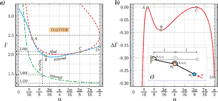
Figure 10: (a) The (dimensionless) follower force $F$, shown as a function of the (transformed via $\cot{\alpha}=m_{1}/m_{2}$) mass ratio $\alpha$, represents the flutter domain of (dashed/red line) the undamped, or ‘ideal’, Ziegler pendulum SW1975 and the flutter boundary of the dissipative system in the limit of vanishing (dot-dashed/green line) internal and (continuous/blue line) external damping. (b) Discrepancy $\Delta F$ between the critical flutter load for the ideal Ziegler pendulum and for the same structure calculated in the limit of vanishing external damping. The discrepancy quantifies the Ziegler’s paradox due to external (air drag) damping T2016 .

In the presence of damping $(b>0)$ the Routh-Hurwitz condition yields the new critical follower load that depends on the square of the damping coefficient $b$

$$P_{k}(b)=\frac{41}{28}\frac{c}{l}+\frac{1}{2}\frac{b^{2}}{ml^{3}}.$$ (47)

Ziegler found that the domain of asymptotic stability for the damped pendulum is given by the inequalities $P<P_{k}(b)$ and $b>0$ and he plotted it against the stability interval $P<P_{k}$ of the undamped system, Figure 9(b). Surprisingly, the limit of the critical load $P_{k}(b)$ when $b$ tends to zero turned out to be significantly lower than the critical load of the undamped system

$$P_{k}^{*}=\lim_{b\rightarrow 0}P_{k}(b)=\frac{41}{28}\frac{c}{l}\simeq 1.464\frac{c}{l}<P_{k}.$$ (48)

Note that in the original work of Ziegler, formula (47) contains a misprint which yields linear dependency of the critical follower load on the damping coefficient $b$. Nevertheless, the domain of asymptotic stability found in Z52 and reproduced in Figure 9(b), is correct.

Ziegler limited his original calculation to a particular mass distribution, $m_{1}=2m_{2}$, and took into account only internal damping in the joints, neglecting, e.g, the air drag (an external damping). Later studies confirmed that the Ziegler paradox is a generic phenomenon and exists at all mass distributions, both for internal and external damping BK2018 ; B2018 ; SLK2019 ; T2016 , see Figure 10.

After invention of robust methods of practical realization of follower forces BN2011 the Ziegler paradox was immediately observed in the recent laboratory experiments BK2018 ; B2018 . Nowadays follower forces find new applications in cytosceletal dynamics BD2016 ; DC2017 and acoustics of friction HG03 . In general, the interest to mathematical models involving nonconservative positional forces (known also as circulatory Z53 or curl BS2016 forces) is growing both in traditional areas such as energy harvesting and fluid-structure interactions HD92 ; PMB2017 and in rapidly emerging new research fields of optomechanics SD2017 and light robotics LR2017 .

3 Bottema’s analysis of Ziegler’s paradox

In 1956, in the journal ‘Indagationes Mathematicae’, there appeared an article by Oene Bottema (1901-1992) B56 , then Rector Magnificus of the Technical University of Delft and an expert in classical geometry and mechanics, that outstripped later findings for decades. Bottema’s work on stability in 1955 B55 can be seen as an introduction, it was directly motivated by Ziegler’s paradox. However, instead of examining the particular model of Ziegler, he studied in B56 a much more general class of non-conservative systems.

Following B55 ; B56 , we consider a holonomic scleronomic linear system with two degrees of freedom, of which the coordinates $x$ and $y$ are chosen in such a way that the kinetic energy is $T=({\dot{x}}^{2}+{\dot{y}}^{2})/2.$ Hence the Lagrange equations of small oscillations near the equilibrium configuration $x=y=0$ are as follows

$$\ddot{x}+a_{11}x+a_{12}y+b_{11}\dot{x}+b_{12}\dot{y} = 0,$$

$$\ddot{y}+a_{21}x+a_{22}y+b_{21}\dot{x}+b_{22}\dot{y} = 0,$$ (49)

where $a_{ij}$ and $b_{ij}$ are constants, ${\bf A}:=(a_{ij})$ is the matrix of the forces depending on the coordinates, ${\bf B}:=(b_{ij})$ of those depending on the velocities. If $\bf A$ is symmetrical and while disregarding the damping associated with the matrix $\bf B$, there exists a potential energy function $V=(a_{11}x^{2}+2a_{12}xy+a_{22}y^{2})/2$, if it is antisymmetrical, the forces are circulatory. When the matrix $\bf B$ is symmetrical, we have a non-gyroscopic damping force, which is positive when the dissipative function $(b_{11}x^{2}+2b_{12}xy+b_{22}y^{2})/2$ is positive definite. If $\bf B$ is antisymmetrical the forces depending on the velocities are purely gyroscopic.

The matrices $\bf A$ and $\bf B$ can both be written uniquely as the sum of symmetrical and antisymmetrical parts: ${\bf A}={\bf K}+{\bf N}$ and ${\bf B}={\bf D}+{\bf G}$, where

$${\bf K}=\left(\begin{array}[]{cc}k_{11}&k_{12}\\ k_{21}&k_{22}\\ \end{array}\right),\quad{\bf N}=\left(\begin{array}[]{rr}0&\nu\\ -\nu&0\\ \end{array}\right),\quad{\bf D}=\left(\begin{array}[]{cc}d_{11}&d_{12}\\ d_{21}&d_{22}\\ \end{array}\right),\quad{\bf G}=\left(\begin{array}[]{rr}0&\Omega\\ -\Omega&0\\ \end{array}\right),$$ (50)

with $k_{11}=a_{11}$, $k_{22}=a_{22}$, $k_{12}=k_{21}=(a_{12}+a_{21})/2$, $\nu=(a_{12}-a_{21})/2$ and $d_{11}=b_{11}$, $d_{22}=b_{22}$, $d_{12}=d_{21}=(b_{12}+b_{21})/2$, $\Omega=(b_{12}-b_{21})/2$.

Disregarding damping, the system (3) has a potential energy function when $\nu=0$, it is purely circulatory for $k_{11}=k_{12}=k_{22}=0$, it is non-gyroscopic for $\Omega=0$, and has no damping when $d_{11}=d_{12}=d_{22}=0$. If damping exists, we suppose in this section that it is positive.

In order to solve the linear stability problem for equations (3) we put $x=C_{1}\exp(\lambda t)$, $y=C_{2}\exp(\lambda t)$ and obtain the characteristic equation for the frequencies of the small oscillations around equilibrium

$$Q:=\lambda^{4}+a_{1}\lambda^{3}+a_{2}\lambda^{2}+a_{3}\lambda+a_{4}=0,$$ (51)

where K03a ; K03b ; K07a

$$a_{1}={\rm tr}{\bf D},\quad a_{2}={\rm tr}{\bf K}+\det{\bf D}+\Omega^{2},\quad a_{3}={\rm tr}{\bf K}{\rm tr}{\bf D}-{\rm tr}{\bf KD}+2\Omega\nu,\quad a_{4}=\det{\bf K}+\nu^{2}.$$ (52)

For the equilibrium to be stable all roots of the characteristic equation (51) must be semi-simple and have real parts which are non-positive.

It is always possible to write, in at least one way, the left hand-side as the product of two quadratic forms with real coefficients, $Q=(\lambda^{2}+p_{1}\lambda+q_{1})(\lambda^{2}+p_{2}\lambda+q_{2}).$ Hence

$$a_{1}=p_{1}+p_{2},\quad a_{2}=p_{1}p_{2}+q_{1}+q_{2},\quad a_{3}=p_{1}q_{2}+p_{2}q_{1},\quad a_{4}=q_{1}q_{2}.$$ (53)

For all the roots of the equation (51) to be in the left side of the complex plane $(L)$ it is obviously necessary and sufficient that $p_{i}$ and $q_{i}$ are positive. Therefore in view of (53) we have: a necessary condition for the roots of $Q=0$ having negative real parts is $a_{i}>0$ $(i=1,2,3,4)$. This system of conditions however is not sufficient, as the example $(\lambda^{2}-\lambda+2)(\lambda^{2}+2\lambda+3)=\lambda^{4}+\lambda^{3}+3\lambda^{2}+\lambda+6$ shows. But if $a_{i}>0$ it is not possible that either one root of three roots lies in $L$ (for then $a_{4}\leq 0$); it is also impossible that no root is in it (for, then $a_{4}\leq 0$). Hence if $a_{i}>0$ at least two roots are in $L$; the other ones are either both in $L$, or both on the imaginary axis, or both in $R$. In order to distinguish between these cases we deduce the condition for two roots being on the imaginary axis. If $\mu i$ ($\mu\neq 0$ is real) is a root, then $\mu^{4}-a_{2}\mu^{2}+a_{4}=0$ and $-a_{1}\mu^{2}+a_{3}=0$. Hence $H:=a_{1}^{2}a_{4}+a_{3}^{2}-a_{1}a_{2}a_{3}=0$. Now by means of (53) we have

$$H=-p_{1}p_{2}(a_{1}a_{3}+(q_{1}-q_{2})^{2}).$$ (54)

In view of $a_{1}>0$, $a_{3}>0$ the second factor is positive; furthermore $a_{1}=p_{1}+p_{2}>0$, hence $p_{1}$ and $p_{2}$ cannot both be negative. Therefore $H<0$ implies $p_{1}>0$, $p_{2}>0$, for $H=0$ we have either $p_{1}=0$ or $p_{2}=0$ (and not both, because $a_{3}>0$), for $H>0$ $p_{1}$ and $p_{2}$ have different signs. We see from the decomposition of the polynomial (51) that all its roots are in $L$ if $p_{1}$ and $p_{2}$ are positive.

Hence: a set of necessary and sufficient conditions for all roots of (51) to be on the left hand-side of the complex plane is

$$a_{i}>0~{}~{}(i=1,2,3,4),\quad H<0.$$ (55)

We now proceed to the cases where all roots have non-positive real parts, so that they lie either in $L$ or on the imaginary axis. If three roots are in $L$ and one on the imaginary axis, this root must be $\lambda=0$. Reasoning along the same lines as before we find that necessary and sufficient conditions for this are $a_{i}>0~{}~{}(i=1,2,3)$, $a_{4}=0$, and $H<0$. If two roots are in $L$ and two (different) roots on the imaginary axis we have $p_{1}>0$, $q_{1}>0$, $p_{2}=0$, $q_{2}>0$ and the conditions are $a_{i}>0~{}~{}(i=1,2,3,4)$ and $H=0$. If one root is in $L$ and three are on the imaginary axis, then $p_{1}>0$, $q_{1}=0$, $p_{2}=0$, $q_{2}>0$ and the conditions are $a_{i}>0~{}~{}(i=1,2,3)$, $a_{4}=0$, and $H=0$.

The obtained conditions are border cases of (55). This does not occur with the last type we have to consider: all roots are on the imaginary axis. We now have $p_{1}=0$, $p_{2}=0$, $q_{1}>0$, $q_{2}>0$. Hence $a_{2}>0$, $a_{4}>0$, $a_{1}=a_{3}=0$ and therefore $H=0$. This set of relations is necessary, but not sufficient, as the example $Q=\lambda^{4}+6\lambda^{2}+25=0$ (which has two roots in $L$ and two in the righthand side of the complex plane $(R)$) shows. The proof given above is not valid because as seen from (55), $H=0$ does not imply now $p_{1}p_{2}=0$, the second factor being zero for $a_{1}a_{3}=0$ and $q_{1}=q_{2}$. The condition can of course easily be given; the equation (51) is $\lambda^{4}+a_{2}\lambda^{2}+a_{4}=0$ and therefore it reads $a_{2}>0$, $a_{4}>0$, $a_{2}^{2}>4a_{4}$.

Summing up we have: all roots of (51) (assumed to be different) have non-positive real parts if and only if one of the two following sets of conditions is satisfied B56

$$A: a_{1}>0,~{}a_{2}>0,~{}a_{3}>0,~{}a_{4}\geq 0,~{}a_{2}\geq\frac{a_{1}^{2}a_{4}+a_{3}^{2}}{a_{1}a_{3}},$$

$$B: a_{1}=0,~{}a_{2}>0,~{}a_{3}=0,~{}a_{4}>0,~{}a_{2}>2\sqrt{a_{4}}.$$ (56)

Note that $a_{1}$ represents the damping coefficients $b_{11}$ and $b_{22}$ in the system. One could expect $B$ to be a limit of $A$, so that for $a_{1}\rightarrow 0$, $a_{3}\rightarrow 0$ the set $A$ would continuously tend to $B$. That is not the case.

Remark first of all that the roots of (51) never lie outside $R$ if $a_{1}=0$, $a_{3}\neq 0$ (or $a_{1}\neq 0$, $a_{3}=0$). Furthermore, if $A$ is satisfied and we take $a_{1}=\varepsilon b_{1}$, $a_{3}=\varepsilon b_{3}$, where $b_{1}$ and $b_{3}$ are fixed and $\varepsilon\rightarrow 0$, the last condition of $A$ reads $(\varepsilon\neq 0)$

$$a_{2}>\frac{b_{1}^{2}a_{4}+b_{3}^{2}}{b_{1}b_{3}}=g_{1}$$

while for $\varepsilon=0$ we have

$$a_{2}>2\sqrt{a_{4}}=g_{2}.$$

Obviously we have B56

$$g_{1}-g_{2}=\frac{(b_{1}\sqrt{a_{4}}-b_{3})^{2}}{b_{1}b_{3}}$$

so that $(g_{1}>g_{2})$ but for $b_{3}=b_{1}\sqrt{a_{4}}$. That means that in all cases where $b_{3}\neq b_{1}\sqrt{a_{4}}$ we have a discontinuity in our stability condition.

In 1987, Leipholz remarked in his monograph on stability theory L1987 that “Independent works of Bottema and Bolotin for second-order systems have shown that in the non-conservative case and for different damping coefficients the stability condition is discontinuous with respect to the undamped case.” However, Leipholz did not mention that, in contrast to Bolotin, Bottema illustrated the phenomenon of the discontinuity in a remarkable geometric diagram, first published in B56 and reproduced in Figure 11.

Following Bottema B56 we substitute in (51) $\lambda=c\mu$, where $c$ is the positive fourth root of $a_{4}>0$. The new equation reads $P:=\mu^{4}+b_{1}\mu^{3}+b_{2}\mu^{2}+b_{3}\mu+1=0$, where $b_{i}=a_{i}/c^{i}$ $(i=1,2,3,4)$. If we substitute $a_{i}=c^{i}b_{i}$ in $A$ and $B$ we get the same condition as when we write $b_{i}$ for $a_{i}$, which was to be expected, because if the roots of (51) are outside $R$, those of $P=0$ are also outside $R$ and inversely. We can therefore restrict ourselves to the case $a_{4}=1$, so that we have only three parameters $a_{1}$, $a_{2}$, $a_{3}$. We take them as coordinates in an orthogonal coordinate system.

The condition $H=0$ or

$$a_{1}a_{2}a_{3}=a_{1}^{2}+a_{3}^{2}$$ (57)

is the equation of a surface $V$ of the third degree, which we have to consider for $a_{1}\geq 0$, $a_{3}\geq 0$, Figure 11. Obviously $V$ is a ruled surface, the line $a_{3}=ma_{1}$, $a_{2}=m+1/m$ $(0<m<\infty)$ being on $V$. The line is parallel to the $0a_{1}a_{3}$-plane and intersects the $a_{2}$-axis in $a_{1}=a_{3}=0$, $a_{2}=m+1/m\geq 2$. The $a_{2}$-axis is the double line of $V$, $a_{2}>2$ being its active part. Two generators pass through each point of it; they coincide for $a_{2}=2$ $(m=1)$, and for $a_{2}\rightarrow\infty$ their directions tend to those of the $a_{1}$ and $a_{3}$-axis $(m=0,m=\infty)$. The conditions $A$ and $B$ express that the image point $(a_{1},a_{2},a_{3})$ lies on $V$ or above $V$. The point $(0,2,0)$ is on $V$, but if we go to the $a_{2}$-axis along the line $a_{3}=ma_{1}$ the coordinate $a_{2}$ has the limit $m+1/m$, which is $>2$ but for $m=1$.

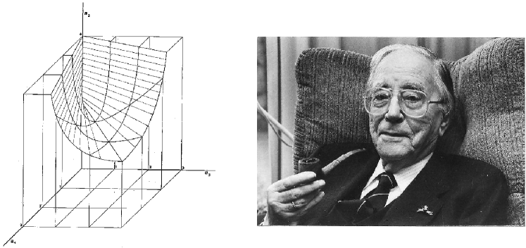
Figure 11: Original drawing (left) from the 1956 work B56 of Oene Bottema (right), showing the domain of the asymptotic stability of the real polynomial of fourth order and of the two-dimensional non-conservative system with Whitney’s umbrella singularity discussed in the sequel. The ruled surface (called $V$ in the text) is given by equation (57).

Note that we started off with 8 parameters in Eq. (3), but that the surface $V$ bounding the stability domain is described by 3 parameters. It is described by a map of $E^{2}$ into $E^{3}$ as in Whitney’s papers W43 ; W44 . Explicitly, a transformation of (19) to (2) is given by

$$a_{1}=\frac{1}{2}y_{3}+w,~{}~{}a_{2}=2+y_{2},~{}~{}a_{3}=-\frac{1}{2}y_{3}+w$$

with $w^{2}=\frac{1}{4}y_{3}^{2}+y_{1}y_{2}$.

Returning to the non-conservative system (3) $(\nu\neq 0)$, with damping, but without gyroscopic forces, so $\Omega=0$, and assuming as in B55 that $k_{12}=0$, $k_{11}>0$, and $k_{22}>0$ (a similar setting but with $d_{12}=0$ and $k_{12}\neq 0$ was considered later by Bolotin in Bo63 ), we find that the condition for stability $H\leq 0$ reads

$$\nu^{2} < \frac{(k_{11}-k_{22})^{2}}{4}$$

$$- \frac{(d_{11}-d_{22})^{2}(k_{11}-k_{22})^{2}-4(k_{11}d_{22}+k_{22}d_{11})(d_{11}d_{22}-d_{12}^{2})(d_{11}+d_{22})}{4(d_{11}+d_{22})^{2}}.$$

Suppose now that the damping force decreases in a uniform way, so we put $d_{11}=\varepsilon d_{11}^{\prime}$, $d_{12}=\varepsilon d_{12}^{\prime}$, $d_{22}=\varepsilon d_{22}^{\prime}$, where $d_{11}$, $d_{12}$, $d_{22}$ are constants and $\varepsilon\rightarrow 0$. Then, for the inequality (3) we get

$$\nu^{2}<\nu_{cr}^{2}:=\frac{(k_{11}-k_{22})^{2}}{4}-\frac{(d_{11}^{\prime}-d_{22}^{\prime})^{2}(k_{11}-k_{22})^{2}}{4(d_{11}^{\prime}+d_{22}^{\prime})^{2}}.$$ (59)

But if there is no damping, we have to make use of condition $B$, which gives

$$\nu^{2}<{\nu_{0}}^{2}:=\frac{(k_{11}-k_{22})^{2}}{4}=\left(\frac{{\rm tr}{\bf K}}{2}\right)^{2}-\det{\bf K}.$$ (60)

Obviously

$${\nu_{0}}^{2}-\nu_{cr}^{2}=\frac{(d_{11}^{\prime}-d_{22}^{\prime})^{2}(k_{11}-k_{22})^{2}}{4(d_{11}^{\prime}+d_{22}^{\prime})^{2}}=\left[\frac{2{\rm tr}{\bf K}{\bf D}-{\rm tr}{\bf K}{\rm tr}{\bf D}}{2{\rm tr}{\bf D}}\right]^{2}\geq 0,$$ (61)

where the expressions written in terms of the invariants of the matrices involved K07a are valid also without the restrictions on the matrices $\bf D$ and $\bf K$ that were adopted in Bo63 ; B55 . For the values of $\frac{2{\rm tr}{\bf K}{\bf D}-{\rm tr}{\bf K}{\rm tr}{\bf D}}{2{\rm tr}{\bf D}}$ which are small with respect to $\nu_{0}$ we can approximately write Ki04 ; K05

$$\nu_{cr}\simeq\nu_{0}-\frac{1}{2\nu_{0}}\left[\frac{2{\rm tr}{\bf K}{\bf D}-{\rm tr}{\bf K}{\rm tr}{\bf D}}{2{\rm tr}{\bf D}}\right]^{2}.$$ (62)

If $\bf D$ depends on two parameters, say $\delta_{1}$ and $\delta_{2}$, then (62) has a canonical form (64) for the Whitney’s umbrella in the $(\delta_{1},\delta_{2},\nu)$-space. Due to discontinuity existing for $2{\rm tr}{\bf K}{\bf D}-{\rm tr}{\bf K}{\rm tr}{\bf D}\neq 0$ the equilibrium may be stable if there is no damping, but unstable if there is damping, however small it may be. We observe also that the critical non-conservative parameter, $\nu_{cr}$, depends on the ratio of the damping coefficients and thus is strongly sensitive to the distribution of damping similarly to how it happens in other applications, including the viscous Chandrasekhar-Friedman-Schutz (CFS) instability of the Maclaurin spheroids LD1977 .

The analytical approximations of the type (62) for the onset of the flutter instability in the general finite-dimensional and infinite-dimensional cases were obtained for the first time in the works K03a ; K03b ; Ki04 ; K05 ; KS05b ; K07b as a result of further development of the sensitivity analysis of simple and multiple eigenvalues in multiparameter families of non-self-adjoint operators. The previous important works include AY75 ; BBM89a ; Br94 ; C95 ; Ha92 ; DS1979 ; J88 ; MK91 ; OR96 ; S1980-2 ; S1980-3 ; S96 ; SKM05 ; Sey . Recent results on the perturbation analysis of dissipation-induced instabilities and the destabilization paradox are summarized in the works K2013dg and LFA2016 .

4 An umbrella without dynamics

Part of global analysis, a topic of pure mathematics, is concerned with singularity theory, which deals with the geometric characterisation and classification of singularities (stationary points) of vector fields. In dynamics these singularities are recognised as equilibria of dynamical systems. Well-known representatives of this singularity school are René Thom Th and Christopher Zeeman. Among pure mathematicians they were exceptional as they promoted singularity theory as useful for real-life problems in biology, the social sciences and physics. Unfortunately their approach gave singularity theory a bad name as in their examples they used geometric methods without explaining a possible relation between realistic vector fields and dynamics. It makes little sense to describe equilibria and transitions (bifurcations) between equilibria without discussing actual causes that are tied in with dynamical processes and corresponding equations of motion. We want to stress here that notwithstanding the lack of dynamics the geometry of singularities as an ingredient of dynamical systems theory can be very useful.

Before Ziegler’s results a geometric result in singularity theory was obtained (1943-44) by Hassler Whitney. This result turned out to be an excellent complement to Bottema’s analytic approach. In his paper W43 , Whitney described singularities of maps of a differential $n$-manifold into $E^{m}$ with $m=2n-1$. It turns out that in this case a special kind of singularity plays a prominent role. Later, the local geometric structure of the manifold near the singularity has been aptly called ‘Whitney’s umbrella’. In Figure 12 we reproduce a sketch of the singular surface.

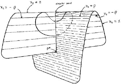
Figure 12: Whitney’s umbrella, lowest dimensional case with 3 parameters W43 ; W44 .

The paper W43 contains two main theorems. Consider the $C^{k}$ map $f:E^{n}\mapsto E^{m}$ with $m=2n-1$.

1. The map $f$ can be altered slightly, forming $f^{*}$, for which the singular points are isolated. For each such an isolated singular point $p$, a technical regularity condition $C$ is valid which relates to the map $f^{*}$ of the independent vectors near $p$ and of the differentials, the vectors in tangent space.

2. Consider the map $f^{*}$ which satisfies condition $C$. Then we can choose coordinates $x=(x_{1},x_{2},\cdots,x_{n})$ in a neighborhood of $p$ and coordinates $y=(y_{1},y_{2},\cdots,y_{m})$ (with $m=2n-1$) in a neighborhood of $y=f(p)$ such that in a neighborhood of $f^{*}(p)$ we have exactly

   $$y_{1} = x_{1}^{2},$$

   $$y_{i} = x_{i},\,\,\,i=2,\cdots,n,$$

   $$y_{n+i-1} = x_{1}x_{i},\,\,\,i=2,\cdots,n.$$

If for instance $n=2,\,m=3$, the simplest interesting case, we have near the origin

$$y_{1}=x_{1}^{2},\,\,y_{2}=x_{2},\,\,y_{3}=x_{1}x_{2},$$ (63)

so that $y_{1}\geq 0$ and on eliminating $x_{1}$ and $x_{2}$:

$$y_{1}y_{2}^{2}-y_{3}^{2}=0.$$ (64)

Starting on the $y_{2}$-axis for $y_{1}=y_{3}=0$, the surface widens up for increasing values of $y_{1}$. For each $y_{2}$, the cross-section is a parabola; as $y_{2}$ passes through $0$, the parabola degenerates to a half-ray, and opens out again (with sense reversed); see Figure 12.

Note that because of the $C^{k}$ assumption for the differentiable map $f$, the analysis is delicate. There is a considerable simplification of the treatment if the map is analytical.

The analysis of singularities of functions and maps is a fundamental ingredient for bifurcation studies of differential equations. After the pioneering work of Hassler Whitney and Marston Morse, it has become a huge research field, both in theoretical investigations and in applications. We can not even present a summary of this field here, so we restrict ourselves to citing a number of survey texts and discussing a few key concepts and examples. In particular we mention AA88 ; Ar71 ; Ar83 ; AA93 ; GS85 ; GS88 ; G1997 ; F1992 . A monograph relating bifurcation theory with normal forms and numerics is Kuz04 .

5 Hopf bifurcation near 1:1 resonance and structural stability

A study of the stability of equilibria of dynamical systems will usually involve the analysis of matrices obtained by linearisation of the equations of motion in a neighbourhood of the equilibria. This triggered off the study of structural stability of matrices as an independent topic in singularity theory Ar71 ; Ar83 .

More explicitly, consider a dynamical system described by the autonomous ODE

$$\dot{\bf x}={\bf f}({\bf x},{\bf p}),\,\,{\bf x}\in{\mathbb{R}}^{n},\,\,{\bf f}:{\mathbb{R}}^{n}\mapsto{\mathbb{R}}^{n},$$

where ${\bf p}\in{\mathbb{R}}^{k}$ is a vector of parameters. An equilibrium ${\bf x}_{0}$ of the system arises if ${\bf f}({\bf x}_{0},{\bf p})={\bf 0}$. With a little smoothness of the map ${\bf f}$ we can linearise near ${\bf x}_{0}$ so that we can write

$$\dot{\bf x}={\bf A}_{\bf p}({\bf x}-{\bf x}_{0})+{\bf g}({\bf x},{\bf p})$$ (65)

with ${\bf A}_{\bf p}$ a constant $n\times n-$ matrix, ${\bf g}({\bf x},{\bf p})$ contains higher-order terms only. In other words

$$\lim_{{\bf x}\rightarrow{\bf x}_{0}}\frac{\|{\bf g}({\bf x},{\bf p})\|}{\|{\bf x}-{\bf x}_{0}\|}=0,$$

${\bf g}({\bf x},{\bf p})$ is tangent to the linear map in ${\bf x}_{0}$. The properties of the matrix ${\bf A}_{\bf p}$ determine in a large number of cases the local behavior of the dynamical system.

Suppose that for ${\bf p}={\bf 0}$, ${\bf A}_{\bf 0}$ has two equal non-zero imaginary eigenvalues and their complex conjugates, $\pm i\omega,\omega>0$, and no other eigenvalues with zero real part. This equilibrium is called a $1:1$ resonant double Hopf point G1997 . (Similarly, in a Hopf point the matrix of linearization has a single conjugate pair of imaginary eigenvalues $\pm i\omega$ and in a double Hopf point there are two distinct such pairs: $\pm i\omega_{1}$, $\pm i\omega_{2}$ G1997 .) Then, without loss of generality, we may assume that the system (65) has been already reduced to a centre manifold of dimension $n=4$. Considering further a generic case of double non-semisimple eigenvalues with geometric multiplicity 1, after a linear change of coordinates and re-scaling time to get $\omega=1$, we can transform ${\bf A}_{\bf 0}$ to F1992

$$\left(\begin{array}[]{rrrr}0&-1&1&0\\ 1&0&0&1\\ 0&0&0&-1\\ 0&0&1&0\\ \end{array}\right).$$ (66)

Setting $z_{1}=\Delta x_{1}+i\Delta x_{2}$ and $z_{2}=\Delta x_{3}+i\Delta x_{4}$, where $i=\sqrt{-1}$ and $\Delta{\bf x}={\bf x}-{\bf x}_{0}$, and assuming ${\bf A}_{\bf 0}$ to be in the form (66) we re-write (65) at ${\bf p}={\bf 0}$ in the complex form F1992

$$\left(\begin{array}[]{c}\dot{z}_{1}\\ \dot{z}_{2}\\ \end{array}\right)=\left(\begin{array}[]{cc}i&1\\ 0&i\\ \end{array}\right)\left(\begin{array}[]{c}z_{1}\\ z_{2}\\ \end{array}\right)+\widetilde{{\bf g}}(z_{1},z_{2},\overline{z}_{1},\overline{z}_{2}).$$ (67)

The second pair of equations governing the conjugates $\overline{z}_{1}$, $\overline{z}_{2}$ is omitted here for simplicity.

Arnold Ar71 ; Ar83 has proven that a universal unfolding of the linear vector field with the matrix

$$\left(\begin{array}[]{cc}i&1\\ 0&i\\ \end{array}\right)$$

is given by the three-parameter family of complex matrices

$$\left(\begin{array}[]{cc}i+\alpha&1\\ \mu_{1}+i\mu_{2}&i+\alpha\\ \end{array}\right),$$ (68)

where $\alpha$, $\mu_{1}$, and $\mu_{2}$ are real parameters and versality is understood with respect to the group of similarity transformations and a real positive scaling. The set of matrices with a resonant Hopf pair is a group orbit G1997 .

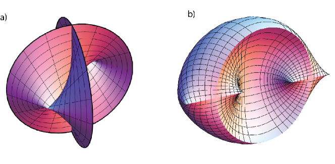
Figure 13: (a) The Plücker conoid in the unfolding of a semisimple $1:1$ resonance has a pair of Whitney umbrellas HK10 ; (b) two pairs of Whitney umbrellas on the boundary of the stability domain of a general 4-degrees-of-freedom dynamical system near a semisimple $1:1$ resonance HK14 .

The universal unfolding has a pure imaginary eigenvalue if and only if there exists a real number $\delta$ such that $(i(\delta-1)-\alpha)^{2}-(\mu_{1}+i\mu_{2})=0$. Eliminating $\delta$ yields G1997

$$\alpha^{2}(−4\mu_{1}+4\alpha^{2})=\mu_{2}^{2}.$$

Setting $y_{2}=\alpha$, $y_{3}=\mu_{2}$, and $y_{1}=−4\mu_{1}+4\alpha^{2}$ we reduce the equation to the form $y_{3}^{2}=y_{1}y_{2}^{2}$, which is nothing else but the normal form (64) for the Whitney umbrella. The double Hopf points of (68) form the half-line $\alpha=\mu_{2}=0$, $\mu_{1}=0$. Along the continuation $\mu_{1}>0$ of this half-line the eigenvalues of (68) are given by $\lambda=i\pm\sqrt{\mu_{1}}$. We see that the double Hopf points have codimension 2 and the resonant double Hopf points are of codimension 3.

If a family of matrices ${\bf A}({\bf p})={\bf A}(p_{1},p_{2},p_{3},\ldots,p_{k})$ has a $1:1$ resonant double Hopf point, the universality of the unfolding (68) means that there exist smooth functions $\alpha({\bf p})$, $\mu_{1}({\bf p})$, $\mu_{1}({\bf p})$, such that the Hopf structure of ${\bf A}({\bf p})$ near the $1:1$ resonant point is the same as the Hopf structure of the unfolding with $\alpha$, $\mu_{1}$, $\mu_{2}$ replaced by $\alpha({\bf p})$, $\mu_{1}({\bf p})$, $\mu_{2}({\bf p})$.

Therefore, the stratified set of Hopf points in the neighborhood of a non-semisimple $1:1$ resonance is a Whitney umbrella in $\bf p$-space too G1997 . The functions $\alpha({\bf p})$, $\mu_{1}({\bf p})$, $\mu_{2}({\bf p})$ can be found approximately as truncated Taylor series with respect to the components of the vector $\bf p$ of the parameters Sey .

Similar stratification of Hopf points near a semisimple $1:1$ resonance involves pairs of Whitney umbrellas forming a Plücker conoid HK10 ; HK14 , see Figure 13.

Hoveijn and Ruijgrok (1995) were the first who applied these ideas to a practical problem exhibiting the Ziegler paradox. Namely, they considered a problem of widening due to dissipation of the zones of the combination resonance YS75 in a system of two parametrically forced coupled oscillators HR95 . The system models a rotating disk with oscillating suspension point introduced in RTV93 . Its linearized equations are

$$\ddot{x}+2\Omega\dot{y}+(1+\varepsilon\cos\omega_{0}t)x+2\varepsilon\mu\dot{x} = 0,$$

$$\ddot{y}+2\Omega\dot{x}+(1+\varepsilon\cos\omega_{0}t)y+2\varepsilon\mu\dot{y} = 0.$$ (69)

It is assumed that for $\varepsilon=0$ the system (5) has two pairs of imaginary eigenvalues $\pm i\omega_{1}$, $\pm i\omega_{2}$ that depend on the parameter $\Omega$ representing the speed of rotation. Of special interest is the case of the sum resonance $\omega_{0}=\omega_{1}+\omega_{2}$.

Let parameters $\delta_{1}$ and $\delta_{2}$ control the detuning of the frequencies $\omega_{1}$ and $\omega_{2}$; then $\delta_{+}=\delta_{1}+\delta_{2}$ and $\delta_{-}=\delta_{1}-\delta_{2}$. The parameter $\delta_{+}$ is small and represents the detuning of the exact sum resonance: $\omega_{0}=\omega_{1}+\omega_{2}+\delta_{+}$ where $\delta_{+}=0$. Parameters $\mu_{1}$ and $\mu_{2}$ control the detuning of the damping from $\mu$; $\mu_{+}=\mu_{1}+\mu_{2}$, $\mu_{-}=\mu_{1}-\mu_{2}$.

The original nonlinear system that has the linearization (5) at zero detuning can be reduced to the following type of equation HR95

$$\dot{\bf z}={\bf A}_{0}{\bf z}+\varepsilon{\bf f}({\bf z},\omega_{0}t;{\bf p}),\quad{\bf z}\in{\mathbb{R}}^{4},$$ (70)

where ${\bf A}_{0}$ is a $4\times 4$ matrix with the eigenvalues $\pm i\omega_{1},\pm i\omega_{2}$. The vector of parameters ${\bf p}=(\delta_{+},\delta_{-},\mu_{+},\mu_{-})$ is used to control detuning from resonance and damping.

The vector-valued function $\bf f$ is $2\pi$-periodic in $\omega_{0}t$ and ${\bf f}(0,\omega_{0}t;{\bf p})={\bf 0}$ for all $t$ and $\bf p$. Since the origin is a stationary point of (70), one may ask how its stability depends on the parameters. Analogous to the case of a single forced oscillator, one can make a planar stability diagram by varying the strength $\varepsilon$ and the frequency $\omega_{0}$ of the forcing while fixing the other parameters. Also in this case one obtains a resonance tongue at $\omega_{0}=\omega_{1}+\omega_{2}$. However if damping is varied, the planar stability diagram does not change continuously RTV93 . For instance, applying zero damping ($\mu=0$, no damping detuning) we find instability of the trivial solution (equilibrium) if

$$|\delta_{+}|\leq 1.$$

For $\mu>0$ the trivial solution is unstable if

$$|\delta_{+}|\leq\omega_{0}\sqrt{\frac{1}{4}-\frac{\mu^{2}}{\omega_{0}^{2}}}.$$

The instability interval depends discontinuously on damping coefficient $\mu$!

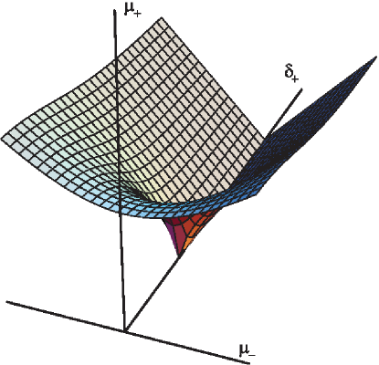
Figure 14: The critical surface for the damped combination resonance in $(\mu_{+},\mu_{-},\delta_{+})$ space, where $\mu_{+}=\mu_{1}+\mu_{2}$, $\mu_{-}=\mu_{1}-\mu_{2}$, $\delta_{+}=\delta_{1}+\delta_{2}$. The parameters $\delta_{1}$ and $\delta_{2}$ control the detuning of the frequencies $\omega_{1}$ and $\omega_{2}$, the parameters $\mu_{1}$ and $\mu_{2}$ the damping of the oscillators. The self-intersection of the surface with the Whitney umbrella singularity is along the $\delta_{+}$ axis HR95 .

Hoveijn and Ruijgrok HR95 presented a geometrical explanation of this dissipation-induced instability using ‘all’ the parameters as unfolding parameters first putting the equation (70) into a normal form Ar83 ; SVM which is similar to that of the non-semisimple $1:1$ resonance studied in F1992 .

In the normalized equation the time dependence appears only in the high order terms. But the autonomous part of this equation contains enough information to determine the stability regions of the origin.

The second step was to test the linear autonomous part ${\bf A}({\bf p})$ of the normalized equation for structural stability. This family of matrices is parameterized by the detunings of the frequencies $\omega_{1}$ and $\omega_{2}$ and of the damping parameter $\mu$.

Identifying the most degenerate member of this family one can show that ${\bf A}({\bf p})$ is its versal unfolding in the sense of Arnold Ar71 ; Ar83 . Put differently, the family ${\bf A}(\delta_{+},\delta_{-},\mu_{+},\mu_{-})$ is structurally stable, whereas ${\bf A}(\delta_{+},\delta_{-},0,0)$ is not. Therefore the stability diagram actually ‘lives’ in a four dimensional space. In this space, the stability regions of the origin are separated by a critical surface which is the hypersurface where ${\bf A}({\bf p})$ has at least one pair of imaginary complex conjugate eigenvalues. This critical surface is diffeomorphic to the Whitney umbrella, see Figure 14.

It is the singularity of the Whitney umbrella that causes the discontinuous behaviour of the planar stability diagram for the combination resonance in the presence of dissipation. The structural stability argument guarantees that the results are ‘universally valid’ and qualitatively hold for every system in sum resonance. For technical details we refer again to HR95 .

6 Abscissa minimization, robust stability and heavy damping

Let us return to the work of Bottema B56 . The conditions

$$a_{1}>0,\quad a_{3}>0,\quad a_{2}>2+\frac{(a_{1}-a_{3})^{2}}{a_{1}a_{3}}>0$$ (71)

are necessary and sufficient for the polynomial

$$p(\lambda)=\lambda^{4}+a_{1}\lambda^{3}+a_{2}\lambda^{2}+a_{3}\lambda+1$$ (72)

to be Hurwitz. The domain (71) was plotted by Bottema in the $(a_{1},a_{3},a_{2})$-space, Figure 15a.

A part of the plane $a_{1}=a_{3}$ that lies inside the domain of asymptotic stability constitutes a set of all directions leading from the point (0, 0, 2) to the stability region

$$\{(a_{1},a_{3},a_{2}):~{}~{}a_{1}=a_{3},~{}~{}a_{1}>0,~{}~{}a_{2}>2\}.$$ (73)

The tangent cone (73) to the domain of asymptotic stability at the Whitney umbrella singularity, which is shown in green in Figure 15a,b, is degenerate in the $(a_{1},a_{3},a_{2})$ – space because it selects a set of measure zero on a unit sphere with the center at the singular point L80 ; L82 .

The singular point $(a_{1},a_{3},a_{2})=(0,0,2)$ corresponds to a double complex-conjugate pair of roots $\lambda=\pm i$ of the polynomial (72). The fact that multiple roots of a polynomial are sensitive to perturbation of the coefficients is a phenomenon that was studied already by Isaac Newton, who introduced the so-called Newton polygon to determine the leading terms of the perturbed roots as fractional powers of a perturbation parameter. It follows that, in matrix analysis, eigenvalues are in general not locally Lipschitz at points in matrix space with non-semi-simple eigenvalues Bu06 , and, in the context of dissipatively perturbed Hamiltonian systems, MO95 . Thus, it has been well-understood for a long time that perturbation of multiple roots or multiple eigenvalues on or near the stability boundary is likely to lead to instability KS05a .

Because of the sensitivity of multiple roots and eigenvalues to perturbation, in engineering and control-theoretical applications a natural desire is to “cut the singularities off” by constructing convex inner approximations to the domain of asymptotic stability. Nevertheless, multiple roots per se are not undesirable.

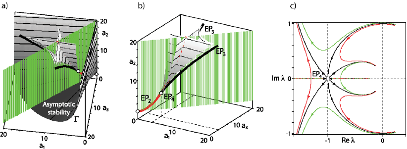
Figure 15: (a) A singular boundary $\Gamma$ of the domain of asymptotic stability (71) of the polynomial (72) with the Whitney umbrella singularity at the point $(a_{1},a_{3},a_{2})=(0,0,2)$, marked by the diamond symbol. (b) The tangent cone, the EP-sets, and the discriminant surface with the Swallowtail singularity at $EP_{4}$. The domain of heavy damping is inside the ‘spire’. (c) Trajectories of roots of the polynomial (72) when $a_{2}$ increases from 0 to 15 and: $a_{1}=a_{3}=4$ (black); $a_{1}=4$, $a_{3}=3.9$ (red); $a_{1}=3.9$, $a_{3}=4$ (green). The global minimum of the abscissa is attained when all the roots coalesce into the quadruple root $\lambda=-1$ ($EP_{4}$) KO2013 .

Indeed, multiple roots also occur deep inside the domain of asymptotic stability. Although it might seem paradoxical at first sight, such configurations are actually obtained by minimizing the so-called polynomial abscissa in an effort to make the asymptotic stability of a linear system more robust, as we now explain.

Abscissa minimization and multiple roots
The abscissa of a polynomial $p(\lambda)$ is the maximal real part of its roots BGMO2012 :

$$a(p)=\max\{{\rm Re}~{}\lambda:~{}~{}p(\lambda)=0\}.$$ (74)

We restrict our attention to monic polynomials with real coefficients and fixed degree $n$: since these have $n$ free coefficients, this space is isomorphic to $\mathbb{R}^{n}$. On this space, the abscissa is a continuous but non-smooth, in fact non-Lipschitz, as well as non-convex, function whose variational properties have been extensively studied using non-smooth variational analysis BGMO2012 ; Bu06 .

Now set $n=4$, consider the set of polynomials $p(\lambda)$ defined in (72), and consider the restricted set of coefficients

$$\left\{(a_{1},a_{3},a_{2}):~{}~{}a_{1}=a_{3},~{}~{}a_{2}=2+\frac{a_{1}^{2}}{4}\right\}$$ (75)

On this set the roots are

$$\lambda_{1}=\lambda_{2}=-\frac{a_{1}}{4}-\frac{1}{4}\sqrt{a_{1}^{2}-16},\quad\lambda_{3}=\lambda_{4}=-\frac{a_{1}}{4}+\frac{1}{4}\sqrt{a_{1}^{2}-16}.$$

When $0\leq a_{1}<4$ $(a_{1}>4)$, the roots $\lambda_{1,2}$ and $\lambda_{3,4}$ are complex (real) with each pair being double, that is with multiplicity two. At $a_{1}=4$ there is a quadruple real eigenvalue $-1$. So, we refer to the set (75) as a set of exceptional points K2013dg ; KI2017 ; KI2018 (abbreviated as the EP-set).

When $a_{1}>0$, the EP-set (75) (shown by the red curve in Figure 15a,b) lies within the tangent cone (73) to the domain of asymptotic stability at the Whitney umbrella singularity $(0,0,2)$. The points in the EP-set all define polynomials with two double roots (denoted $EP_{2}$) except $(a_{1},a_{3},a_{2})=(4,4,6)$, at which $p$ has a quadruple root and is denoted $EP_{4}$; see Figure 15a,b.

Let us consider how the roots move in the complex plane when $a_{1}$ and $a_{3}$ coincide and are set to specific values and $a_{2}$ increases from zero, as shown by black curves in Figure 15c. When $a_{1}=a_{3}<4$, the roots that initially have positive real parts and thus correspond to unstable solutions move along the unit circle to the left, cross the imaginary axis at $a_{2}=2$ and merge with another complex conjugate pair of roots at $a_{2}=2+\frac{a_{1}^{2}}{4}$, i.e., at the EP-set. Further increase in $a_{2}$ leads to the splitting of the double eigenvalues, with one conjugate pair of roots moving back toward the imaginary axis. By also considering the case $a_{1}=a_{3}>4$, it is clear that when $a_{1}$ and $a_{3}$ coincide, the choice $a_{2}=2+\frac{a_{1}^{2}}{4}$ minimizes the abscissa, with the polynomial $p$ on the EP-set.

Furthermore, when $a_{1}=a_{3}$ is increased toward $4$ from below, the coalescence points ($EP_{2}$) move around the unit circle to the left. This conjugate pair of coalescence points merges into the quadruple real root $\lambda=-1$ ($EP_{4}$) when $a_{1}=a_{3}=4$ and hence $a_{2}=6$, as is visible in Figure 15c. If $a_{1}=a_{3}$ is increased above 4 the quadruple point $EP_{4}$ splits again into two exceptional points $EP_{2}$, one of them inside the unit circle.

Thus, all indications are that the abscissa is minimized by the parameters corresponding to $EP_{4}$, with a quadruple root at $-1$.

In fact, application of the following theorem shows that the abscissa of (72) is globally minimized by the $EP_{4}$ parameters.

Theorem 6.1

(BGMO2012 , Theorems 7 and 14)

Let $\mathbb{F}$ denote either the real field $\mathbb{R}$ or the complex field $\mathbb{C}$. Let $b_{0}$, $b_{1}$, $\ldots$, $b_{n}\in\mathbb{F}$ be given (with $b_{1},\ldots,b_{n}$ not all zero) and consider the following family of monic polynomials of degree $n$ subject to a single affine constraint on the coefficients:

$$P=\left\{\lambda^{n}+a_{1}\lambda^{n-1}+\ldots+a_{n-1}\lambda+a_{n}:\quad b_{0}+\sum_{j=1}^{n}b_{j}a_{j}=0,\quad a_{i}\in\mathbb{F}\right\}.$$

Define the optimization problem

$$a^{*}:=\inf_{p\in P}a(p).$$ (76)

Let

$$h(\lambda)=b_{n}\lambda^{n}+b_{n-1}\left(\begin{array}[]{c}n\\ n-1\\ \end{array}\right)\lambda^{n-1}+\ldots+b_{1}\left(\begin{array}[]{c}n\\ 1\\ \end{array}\right)\lambda+b_{0}.$$

First, suppose $\mathbb{F}=\mathbb{R}$. Then, the optimization problem (76) has the infimal value

$$a^{*}=-\max\left\{\zeta\in\mathbb{R}:~{}~{}h^{(i)}(\zeta)=0~{}~{}for~{}~{}some~{}~{}i\in\{0,\ldots,k-1\}\right\},$$

where $h^{(i)}$ is the $i$-th derivative of $h$ and $k=\max\{j:~{}~{}b_{j}\neq 0\}$. Furthermore, the optimal value $a^{*}$ is attained by a minimizing polynomial $p^{*}$ if and only if $-a^{*}$ is a root of $h$ (as opposed to one of its derivatives), and in this case we can take

$$p^{*}(\lambda)=(\lambda-\gamma)^{n}\in P,\quad\gamma=a^{*}.$$

Second, suppose $\mathbb{F}=\mathbb{C}$. Then, the optimization problem (76) always has an optimal solution of the form

$$p^{*}(\lambda)=(\lambda-\gamma)^{n}\in P,\quad{\rm Re}~{}\gamma=a^{*},$$

with $-\gamma$ given by a root of $h$ (not its derivatives) with largest real part.

In our case, $\mathbb{F}=\mathbb{R}$, $n=4$ and the affine constraint on the coefficients of $p$ is simply $a_{4}=1$. So, the polynomial $h$ is given by $h(\lambda)=\lambda^{4}-1$.

Its real root with largest real part is 1, and its derivatives have only the zero root. So, the infimum of the abscissa $a$ over the polynomials (72) is $-1$, and this is attained by

$$p^{*}(\lambda)=(\lambda+1)^{4}=\lambda^{4}+4\lambda^{3}+6\lambda^{2}+4\lambda+1,$$ (77)

that is, with the coefficients at the exceptional point $EP_{4}$. There is nothing special about $n=4$ here; if we replace $4$ by $n$ we find that the infimum is still $-1$ and is attained by

$$p^{*}(\lambda)=(\lambda+1)^{n}.$$

Swallowtail singularity as the global minimizer of the abscissa

It is instructive to understand the set in the $(a_{1},a_{3},a_{2})$-space where the roots of the polynomial (72) are real and negative, but not necessarily simple, which is given by the discriminant surface of the polynomial. A part of it is shown in Figure 15a,b. At the point $EP_{4}$ with the coordinates $(4,4,6)$ in the $(a_{1},a_{3},a_{2})$- space the discriminant surface has the Swallowtail singularity, which is a generic singularity of bifurcation diagrams in three-parameter families of real matrices Ar71 ; Ar83 .

Therefore, the coefficients of the globally minimizing polynomial (77) are exactly at the Swallowtail singularity of the discriminant surface of the polynomial (72).

In the region in side the “spire” formed by the discriminant surface all the roots are simple real and negative. Owing to this property, this region, belonging to the domain of asymptotic stability (see Figure 15a), plays an important role in stability theory. Physical systems with semi-simple real and negative eigenvalues are called heavily damped. The solutions of the heavily damped systems do not oscillate and monotonically decrease, which is favorable for applications in robotics and automatic control.

Now we can give the following interpretation of the Bottema stability diagram shown in Figure 15a KO2013 . The dissipative system with the characteristic polynomial (72) is asymptotically stable inside the domain (71). The boundary of the domain (72) has the Whitney umbrella singular point at $a_{1}=0$, $a_{3}=0$, and $a_{2}=2$.

The domain corresponding to heavily damped systems is confined between three hypersurfaces of the discriminant surface and has a form of a trihedral spire with the Swallowtail singularity at its cusp at $a_{1}=4$, $a_{2}=6$, and $a_{3}=4$. The Whitney umbrella and the Swallowtail singular points are connected by the EP-set given by (75). At the Swallowtail singularity of the boundary of the domain of heavily damped systems, the abscissa of the characteristic polynomial of the damped system attains its global minimum.

Therefore, by minimizing the spectral abscissa one finds points at the boundary of the domain of heavily damped systems. Furthermore, the sharpest singularity at this boundary corresponding to a quadruple real eigenvalue $\lambda=-1$ with the Jordan block of order four is the very point where all the modes of the system with two degrees of freedom are decaying to zero as rapidly as possible when $t\rightarrow\infty$.

References

- (1) Abbott, B. P., et al.: (LIGO Scientific Collaboration and Virgo Collaboration) GW170817: Observation of gravitational waves from a binary neutron star inspiral. Phys. Rev. Lett. 119, 161101 (2017)
- (2) Alfriend, K. T.: The stability of the triangular Lagrangian points for commensurability of order two. Celest. Mech. 1(3–4), 351–359 (1970)
- (3) Andersson, N.: Gravitational waves from instabilities in relativistic stars. Class. Quantum Grav. 20, R105–R144 (2003)
- (4) Andreichikov, I. P., Yudovich, V. I.: The stability of visco-elastic rods. Izv. Akad. Nauk SSSR. Mekhanika Tverdogo Tela. 9(2), 78–87 (1974)
- (5) Anosov, D. V., Arnold, V. I. (eds.): Dynamical Systems I, Encyclopaedia of Mathematical Sciences, Springer, Berlin, (1988)
- (6) Arnold, V. I.: Lectures on bifurcations in versal families. Russ. Math. Surv. 27, 54–123 (1972)
- (7) Arnold, V. I.: Geometrical Methods in the Theory of Ordinary Differential Equations, Springer-Verlag, New York, (1983)
- (8) Arnold, V. I. (ed.): Dynamical Systems VIII, Encyclopaedia of Mathematical Sciences, Springer, Berlin, (1993)
- (9) Bayly, P. V., Dutcher, S. K.: Steady dynein forces induce flutter instability and propagating waves in mathematical models of flagella. J. R. Soc. Interface 13, 20160523 (2016)
- (10) Berry, M. V., Shukla, P.: Curl force dynamics: symmetries, chaos and constants of motion. New J. Phys. 18, 063018 (2016)
- (11) Banichuk, N. V., Bratus, A. S., Myshkis, A. D.: On destabilizing influence of small dissipative forces to nonconservative systems. Doklady AN SSSR 309(6), 1325–1327 (1989)
- (12) Bialynicki-Birula, I., Kalinski, M., Eberly, J. H.: Lagrange equilibrium points in celestial mechanics and nonspreading wave packets for strongly driven Rydberg electrons. Phys. Rev. Lett. 73(13), 1777–1780 (1994)
- (13) Bialynicki-Birula, I., Charzyǹski, S.: Trapping and guiding bodies by gravitational waves endowed with angular momentum. Phys. Rev. Lett. 121, 171101 (2018)
- (14) Bigoni, D., Noselli, G. Experimental evidence of flutter and divergence instabilities induced by dry friction. J. Mech. Phys. Sol. 59, 2208–2226 (2011)
- (15) Bigoni, D., Kirillov, O. N., Misseroni, D., Noselli, G., Tommasini, M.: Flutter and divergence instability in the Pflüger column: Experimental evidence of the Ziegler destabilization paradox. J. Mech. Phys. Sol. 116, 99–116 (2018)
- (16) Bigoni, D., Misseroni, D., Tommasini, M., Kirillov, O. N., Noselli, G. Detecting singular weak-dissipation limit for flutter onset in reversible systems. Phys. Rev. E 97(2), 023003 (2018)
- (17) Bloch, A. M., Krishnaprasad, P. S., Marsden, J. E., Ratiu, T. S.: Dissipation-induced instabilities. Annales de l’Institut Henri 11(1), 37–90 (1994)
- (18) Blondel, V. D., Gürbüzbalaban, M., Megretski, A., Overton, M. L.: Explicit solutions for root optimization of a polynomial family with one affine constraint. IEEE Trans. Autom. Control 57, 3078–3089 (2012)
- (19) Bognár, J.: Indefinite inner product spaces, Springer, New York (1974)
- (20) Bolotin, V. V.: Non-conservative Problems of the Theory of Elastic Stability. Fizmatgiz (in Russian), Moscow (1961); Pergamon, Oxford (1963)
- (21) Bolotin, V. V., Zhinzher, N. I.: Effects of damping on stability of elastic systems subjected to nonconservative forces. Int. J. Solids Struct. 5, 965–989 (1969)
- (22) Borisov, A. V., Kilin, A. A., Mamaev, I. S.: The Hamiltonian dynamics of self-gravitating liquid and gas ellipsoids. Reg. Chaot. Dyn. 14(2), 179–217 (2009)
- (23) Bottema, O.: On the stability of the equilibrium of a linear mechanical system. Z. Angew. Math. Phys. 6, 97–104 (1955)
- (24) Bottema, O.: The Routh-Hurwitz condition for the biquadratic equation. Indag. Math. 59, 403–406 (1956)
- (25) Bottema, O. Stability of equilibrium of a heavy particle on a rotating surface. Z. angew. Math. Phys. 27, 663–669 (1976)
- (26) Bridges, T. J., Dias, F.: Enhancement of the Benjamin-Feir instability with dissipation. Phys. Fluids 19, 104104 (2007)
- (27) Brouwer, L. E. J.: The motion of a particle on the bottom of a rotating vessel under the influence of the gravitational force, (Dutch). Nieuw Arch. v. Wisk., 2e reeks 12, 407–419 (1918) (English transl. in collected works B76 , North-Holland Publ. 1976)
- (28) Brouwer, L. E. J. : Collected Works vol. 2, Geometry, Analysis, Topology and Mechanics, Freudenthal, H., ed., North-Holland, Amsterdam (1976)
- (29) Burke, J. V., Henrion, D., Lewis, A. S., Overton, M. L.: Stabilization via nonsmooth, nonconvex optimization. IEEE Trans. Autom. Control 51(11), 1760–1769 (2006)
- (30) Chandrasekhar, S.: Ellipsoidal Figures of Equilibrium. Yale University Press, New Haven (1969)
- (31) Chandrasekhar, S.: Solutions of two problems in the theory of gravitational radiation. Phys. Rev. Lett. 24(11), 611–615 (1970)
- (32) Chandrasekhar, S.: On stars, their evolution and their stability. Science 226(4674), 497–505 (1984)
- (33) Cox, G., Levi, M.: Gaussian curvature and gyroscopes. Comm. Pure Appl. Math., 71, 938–952 (2018)
- (34) Crandall, S. H.: The effect of damping on the stability of gyroscopic pendulums. Z. angew. Math. Phys. 46, S761–S780 (1995)
- (35) De Canio, G., Lauga, E., Goldstein, R. E.: Spontaneous oscillations of elastic filaments induced by molecular motors. J. R. Soc. Interface 14, 20170491 (2017)
- (36) Dyson, J., Schutz, B. F.: Perturbations and stability of rotating stars-I. Completeness of normal modes. Proc. R. Soc. Lond. A 368, 389–410 (1979)
- (37) Gascheau, G.: Examen d’une classe d’equations differentielles et application á un cas particulier du probleme des trois corps. C. R. Acad. Sci. 16, 393–394 (1843)
- (38) Gladwell, G.: Follower forces – Leipholz early researches in elastic stability. Can. J. Civil Eng. 17, 277–286 (1990)
- (39) Golubitsky, M., Schaeffer, D. G.: Singularities and maps in bifurcation theory. vol. 1, Applied Mathematical Sciences 51, Springer, Berlin (1985)
- (40) Golubitsky, M., Schaeffer, D. G., Stewart, I.: Singularities and maps in bifurcation theory. vol. 2, Applied Mathematical Sciences 69, Springer, Berlin (19880
- (41) Govaerts, W., Guckenheimer, J., Khibnik, A.: Defining functions for multiple Hopf bifurcations. SIAM J. Numer. Anal. 34(3), 1269–1288 (1997)
- (42) Greenhill, A. G.: On the general motion of a liquid ellipsoid under the gravitation of its own parts. Proc. Cambridge Philos. Soc. 4, 4–14 (1880)
- (43) Greenhill, A. G.: On the strength of shafting when exposed both to torsion and to end thrust. Proc. Inst. Mech. Eng. 34, 182–225 (1883)
- (44) Haller, G.: Gyroscopic stability and its loss in systems with two essential coordinates. Intern. J. of Nonl. Mechs. 27, 113–127 (1992)
- (45) Heisenberg, W.: Über Stabilität und Turbulenz von Flüssigkeitsströmen. Ann. Phys. 379, 577–627 (1924)
- (46) Hoffmann, N., Gaul, L.: Effects of damping on mode-coupling instability in friction-induced oscillations. Z. angew. Math. Mech. 83, 524–534 (2003)
- (47) Holopäinen, E. O.: On the effect of friction in baroclinic waves. Tellus. 13(3), 363–367 (1961)
- (48) Hoveijn, I., Ruijgrok, M.: The stability of parametrically forced coupled oscillators in sum resonance. Z. angew. Math. Phys., 46, 384–392 (1995)
- (49) Hoveijn, I., Kirillov, O. N.: Singularities on the boundary of the stability domain near 1:1-resonance. J. Diff. Eqns, 248(10), 2585–2607 (2010)
- (50) Hoveijn, I., Kirillov, O.: Determining the stability domain of perturbed four-dimensional systems in 1:1 resonance. in “Nonlinear Physical Systems: Spectral Analysis, Stability and Bifurcations” (eds. Kirillov, O. and Pelinovsky, D.), Wiley-ISTE, London, Chapter 8: 155–175 (2014)
- (51) Iooss, G., Adelmeyer, M.: Topics in bifurcation theory. World Scientific, Singapore (1992)
- (52) Jones, C. A.: Multiple eigenvalues and mode classification in plane Poiseuille flow. Q. J. Mech. appl. Math., 41(3), 363–382 (1988)
- (53) Kirillov, O. N.: How do small velocity-dependent forces (de)stabilize a non-conservative system? DCAMM Report. No. 681. April 2003. 40 pages.
- (54) Kirillov, O. N.: How do small velocity-dependent forces (de)stabilize a non-conservative system? Proceedings of the International Conference ”Physics and Control”. St.-Petersburg. Russia. August 20-22. Vol. 4, 1090–1095 (2003).
- (55) Kirillov, O. N.: Destabilization paradox. Doklady Physics. 49(4), 239–245 (2004)
- (56) Kirillov, O. N.: A theory of the destabilization paradox in non-conservative systems. Acta Mechanica. 174(3-4), 145–166 (2005)
- (57) Kirillov, O. N., Seyranian, A. P.: Stabilization and destabilization of a circulatory system by small velocity-dependent forces. J. Sound Vibr. 283(3-5), 781–800 (2005)
- (58) Kirillov, O. N., Seyranian, A. O.: The effect of small internal and external damping on the stability of distributed non-conservative systems. J. Appl. Math. Mech. 69(4), 529–552 (2005)
- (59) Kirillov, O. N.: Destabilization paradox due to breaking the Hamiltonian and reversible symmetry. Int. J. Non-Lin. Mech. 42(1), 71–87 (2007)
- (60) Kirillov, O. N.: Gyroscopic stabilization in the presence of nonconservative forces. Dokl. Math. 76(2), 780–785 (2007)
- (61) Kirillov, O. N.: Campbell diagrams of weakly anisotropic flexible rotors. Proc. of the Royal Society A 465(2109), 2703–2723 (2009)
- (62) Kirillov, O. N., Verhulst, F.: Paradoxes of dissipation-induced instability or who opened Whitney’s umbrella? Z. angew. Math. Mech. 90, 462–488 (2010)
- (63) Kirillov, O. N.: Brouwer’s problem on a heavy particle in a rotating vessel: wave propagation, ion traps, and rotor dynamics. Phys. Lett. A 375, 1653–1660 (2011)
- (64) Kirillov, O. N.: Nonconservative Stability Problems of Modern Physics. De Gruyter Studies in Mathematical Physics 14, De Gruyter, Berlin, Boston (2013)
- (65) Kirillov, O. N.: Stabilizing and destabilizing perturbations of PT-symmetric indefinitely damped systems. Phil. Trans. R. Soc. A 371, 20120051 (2013)
- (66) Kirillov, O. N.: Singular diffusionless limits of double-diffusive instabilities in magnetohydrodynamics. Proc. R. Soc. A 473(2205), 20170344 (2017)
- (67) Kirillov, O. N. Locating the sets of exceptional points in dissipative systems and the self-stability of bicycles. Entropy 20(7), 502 (2018)
- (68) Kirillov, O. N., Levi, M.: A Coriolis force in an inertial frame. Nonlinearity 30(3), 1109–1119 (2017)
- (69) Kirillov, O. N., Overton, M. L.: Robust stability at the swallowtail singularity. Frontiers in Physics 1, 24 (2013)
- (70) Kollàr, R., Miller, P. D.: Graphical Krein signature theory and Evans-Krein functions. SIAM Review 56(1), 73–123 (2014)
- (71) Kopachevskii, N. D., Krein, S. G.: Operator Approach in Linear Problems of Hydrodynamics. Self-adjoint Problems for an Ideal Fluid, Operator Theory: Advances and Applications 1, Birkhauser, Basel (2001)
- (72) Krechetnikov, R., Marsden, J. E.: Dissipation-induced instabilities in finite dimensions. Rev. Mod. Phys. 79, 519–553 (2007)
- (73) Krein, M. G.: Topics in differential and integral equations and operator theory, Operator Theory 7, Birkhauser, Basel (1983)
- (74) Kuznetsov, Yu. A.: Elements of applied bifurcation theory, Applied Mathematical Sciences 112, Springer, Berlin (2004)
- (75) Lamb, H.: On kinetic stability. Proc. R. Soc. London A 80(537), 168–177 (1908)
- (76) Lancaster, P.: Stability of linear gyroscopic systems: a review. Lin. Alg. Appl. 439, 686–706 (2013)
- (77) Langford, W. F.: Hopf meets Hamilton under Whitney’s umbrella. In: IUTAM symposium on nonlinear stochastic dynamics. Proceedings of the IUTAM symposium, Monticello, IL, USA, Augsut 26-30, 2002, Solid Mech. Appl. 110, S. N. Namachchivaya, et al., eds., pp. 157–165, Kluwer, Dordrecht (2003)
- (78) Lebovitz, N. R.: Binary fission via inviscid trajectories. Geoph. Astroph. Fluid. Dyn. 38(1), 15–24 (1987)
- (79) Leipholz, H.: Stability theory: an introduction to the stability of dynamic systems and rigid bodies. 2nd ed., Teubner, Stuttgart (1987)
- (80) Levantovskii, L. V.: The boundary of a set of stable matrices. Uspekhi Mat. Nauk 35, no. 2(212), 213–214 (1980)
- (81) Levantovskii, L. V.: Singularities of the boundary of a region of stability, (Russian). Funktsional. Anal. i Prilozhen. 16, no. 1, 44–48, 96 (1982)
- (82) Lindblom, L., Detweiler, S. L.: On the secular instabilities of the Maclaurin spheroids. Astrophys. J. 211, 565–567 (1977)
- (83) Liouville, J.: Memoire sur les figures ellipsoïdales a trois axes inegaux, qui peuvent convenir a l’equilibre d’une masse liquide homogene, douee d’un mouvement de rotation. Journal de mathematiques pures et appliquees. 1re serie, tome 16, 241–254 (1851)
- (84) Luongo, A., Ferretti, M., D’Annibale, F.: Paradoxes in dynamic stability of mechanical systems: investigating the causes and detecting the nonlinear behaviors. Springer Plus. 5, 60 (2016)
- (85) Lyapunov, A. M.: The general problem of the stability of motion (translated into English by A. T. Fuller). Int. J. Control. 55, 531–773 (1992)
- (86) MacKay, R. S.: Stability of equilibria of Hamiltonian systems. In: Nonlinear Phenomena and Chaos, (ed. S. Sarkar), Adam Hilger, Bristol, pp. 254–270 (1986)
- (87) MacKay, R. S. Movement of eigenvalues of Hamiltonian equilibria under non-Hamiltonian perturbation. Phys. Lett. A 155, 266–268 (1991)
- (88) Maclaurin, C. A. A Treatise of Fluxions: In Two Books. 1. Vol. 1. Ruddimans (1742)
- (89) Maddocks, J., Overton, M. L.: Stability theory for dissipatively perturbed Hamiltonian systems. Comm. Pure and Applied Math. 48, 583–610 (1995)
- (90) McHugh, K. A., Dowell, E. H.: Nonlinear response of an inextensible, cantilevered beam subjected to a nonconservative follower force. J. Comput. Nonlinear Dynam. 14(3), 031004 (2019)
- (91) McIntyre, M. E.: Diffusive destabilisation of the baroclinic circular vortex. Geophys. Astrophys. Fluid Dyn. 1(1-2), 19–57 (1970)
- (92) Meyer, C. O.: De aequilibrii formis ellipsoidicis. J. Reine Angew. Math. 24, 44–59 (1842)
- (93) Montgomery, M.: Hartmann, Lundquist, and Reynolds: the role of dimensionless numbers in nonlinear magnetofluid behavior. Plasma Phys. Control. Fusion 35, B105–B113 (1993)
- (94) Nezlin, M. V.: Negative-energy waves and the anomalous Doppler effect. Soviet Physics Uspekhi. 19, 946–954 (1976)
- (95) Nicolai, E. L.: On the stability of the rectilinear form of equilibrium of a bar in compression and torsion. Izvestia Leningradskogo Politechnicheskogo Instituta. 31, 201–231 (1928)
- (96) O’Reilly, O. M., Malhotra, N. K.,Namachchivaya, N. S.: Some aspects of destabilization in reversible dynamical systems with application to follower forces. Nonlin. Dyn. 10, 63–87 (1996)
- (97) Perego, A. M., Turitsyn, S. K., Staliunas, K.: Gain through losses in nonlinear optics, Light: Science and Applications 7, 43 (2018)
- (98) Phillips, D., Simpson, S., Hanna, S.: Chapter 3 - Optomechanical microtools and shape-induced forces, in: Light Robotics: Structure-Mediated Nanobiophotonics, Glückstad, J., Palima, D. eds., Elsevier, Amsterdam, pp. 65–98 (2017)
- (99) Pigolotti, L., Mannini, C., Bartoli, G.: Destabilizing effect of damping on the post-critical flutter oscillations of flat plates. Meccanica 52(13), 3149–3164 (2017)
- (100) Poincaré, H.: Leçons sur les hypothèses cosmogoniques (ed. Henri Vergne), Librairie Scientifique A. Hermann et fils, Paris (1913)
- (101) Pontryagin, L.: Hermitian operators in a space with indefinite metric. Izv. Akad. Nauk. SSSR Ser. Mat. 8, 243–280 (1944)
- (102) Riemann, B.: Ein Beitrag zu den Untersuchungen über die Bewegung eines gleichartigen flüssigen ellipsoides. Abh. d. Königl. Gesell. der Wiss. zu Göttingen. 9, 3–36 (1861)
- (103) Roberts, G. E.: Linear stability of the elliptic Lagrangian triangle solutions in the three-body problem. J. Diff. Eqns 182, 191–218 (2002)
- (104) Roberts, R. H., Stewartson, K.: On the stability of a Maclaurin spheroid of small viscosity. Astrophys. J. 137, 777–790 (1963)
- (105) Ruijgrok, M., Tondl, A., Verhulst, F.: Resonance in a Rigid Rotor with Elastic Support. Z. angew. Math. Mech. 73, 255–263 (1993)
- (106) Samantaray, A. K., Bhattacharyya, R., Mukherjee, A.: On the stability of Crandall gyropendulum. Phys. Lett. A 372, 238–243 (2008)
- (107) Sanders, J. A., Verhulst, F., Murdock, J.: Averaging methods in nonlinear dynamical systems. Applied Math. Sciences 59, Springer, Berlin (2007)
- (108) Saw, S. S., Wood, W. G.: The stability of a damped elastic system with a follower force. J. Mech. Eng. Sci. 17(3), 163–176 (1975)
- (109) Schindler, J., Li, A., Zheng, M. C., Ellis, F. M., Kottos, T.: Experimental study of active LRC circuits with PT symmetries. Phys. Rev. A 84, 040101(R) (2011)
- (110) Schutz, B. F.: Perturbations and stability of rotating stars-II. Properties of the eigenvectors and a variational principle. Mon. Not. R. astr. Soc. 190, 7–20 (1980)
- (111) Schutz, B. F.: Perturbations and stability of rotating stars-III. Perturbation theory for eigenvalues. Mon. Not. R. astr. Soc. 190, 21–31 (1980)
- (112) Seyranian, A. P.: On stabilization of non-conservative systems by dissipative forces and uncertainty of critical load. Doklady Akademii Nauk. 348, 323–326 (1996)
- (113) Seyranian, A. P., Kirillov, O. N., Mailybaev, A. A.: Coupling of eigenvalues of complex matrices at diabolic and exceptional points. J. Phys. A: Math. Gen. 38(8), 1723–1740 (2005)
- (114) Seyranian, A. P., Mailybaev, A. A.: Multiparameter stability theory with mechanical applications. World Scientific, Singapore (2003)
- (115) Shapiro, V. E. The gyro force of high-frequency fields lost by the concept of effective potential. Phys. Lett. A 238, 147–152 (1998)
- (116) Sinou, J.-J., Jezequel, L.: Mode coupling instability in friction-induced vibrations and its dependency on system parameters including damping. Eur. J. Mech. A. 26, 106–122 (2007)
- (117) Smith, D. M.: The motion of a rotor carried by a flexible shaft in flexible bearings. Proc. Roy. Soc. London A 142, 92–118 (1933)
- (118) Sobolev, S. On motion of a symmetric top with a cavity filled with fluid. in: G. V. Demidenko and V. L. Vaskevich (eds.), Selected Works of S. L. Sobolev, pp. 333–382, Springer (2006)
- (119) Stewartson, K.: On the stability of a spinning top containing liquid. J. Fluid Mech. 5, 577–592 (1959)
- (120) Sturrock, P. A.: Kinematics of growing waves. Phys. Rev. 112, 1488–1503 (1958)
- (121) Sturrock, P. A.: In what sense do slow waves carry negative energy. J. Appl. Phys. 31, 2052–2056 (1960)
- (122) Sugiyama, Y., Langthjem, M., Katayama, K.: Dynamic Stability of Columns under Nonconservative Forces: Theory and Experiment. Solid Mechanics and its Applications 255, Springer, Berlin (2019)
- (123) Sukhov, S., Dogariu, A.: Non-conservative optical forces. Rep. Prog. Phys. 80, 112001 (2017)
- (124) Thom, R.: Structural Stability and Morphogenesis, W. A. Benjamin (1972)
- (125) Thomson, W., Tait, P. G.: Treatise on Natural Philosophy, Vol. I, Part I, New Edition, Cambridge Univ. Press, Cambridge, pp. 387–391 (1879)
- (126) Thompson, J. M. T.: Instabilities of elastic and spinning systems: concepts and phenomena. Int. J. Bif. Chaos. 27(09), 1730029 (2017)
- (127) Thomson, W.: On an experimental illustration of minimum energy. Nature 23, 69–70 (1880)
- (128) Thorpe, S. A., Smyth, W. D., Li, L.: The efect of small viscosity and diffusivity on the marginal stability of stably stratified shear flows. J. Fluid. Mech. 731, 461–476 (2013)
- (129) Tommasini, M., Kirillov, O. N., Misseroni, D., Bigoni, D.: The destabilizing effect of external damping: Singular flutter boundary for the Pflüger column with vanishing external dissipation. J. Mech. Phys. Sol. 91, 204–215 (2016)
- (130) Verhulst, F.: Parametric and Autoparametric Resonance. Acta Appl. Math. 70(1-3), 231–264 (2002)
- (131) Verhulst, F.: Perturbation analysis of parametric resonance. Encyclopedia of Complexity and Systems Science, Springer, Berlin (2009)
- (132) van Gils, S. A., Krupa, M., Langford, W. F.: Hopf bifurcation with non-semisimple 1:1 resonance. Nonlinearity 3, 825–850 (1990)
- (133) von Laue, M.: Die Fortpflanzung der Strahlung in dispergierenden und absorbierenden Medien. Ann. Physik 18(4), 523–566 (1905)
- (134) Whitney, H.: The general type of singularity of a set of smooth functions of variables. Duke Math. J. 10, 161–172 (1943)
- (135) Whitney, H.: The singularities of a smooth -manifold in -space. Ann. of Math. 45(2), 247–293 (1944)
- (136) Williamson, J.: On the algebraic problem concerning the normal forms of linear dynamical systems. American Journal of Mathematics. 58, 141–163 (1936)
- (137) Williamson, J.: On the normal forms of linear canonical transformations in dynamics. American Journal of Mathematics. 59, 599–617 (1937)
- (138) Willcocks, B. T., Esler, J. G.: Nonlinear baroclinic equilibration in the presence of Ekman friction. J. Phys. Oceanogr. 42, 225–242 (2012)
- (139) Yakubovich, V. A., Starzhinskii, V. M.: Linear differential equations with periodic coefficients. 2 vols., John Wiley, New York (1975)
- (140) Yang, C., Khesin, B.: Averaging, symplectic reduction, and central extensions. arXiv:1806.01755 (2018)
- (141) Yurkin, M. Y.: The finite dimension property of small oscillations of a top with a cavity filled with an ideal fluid. Funct. Anal. Appl. 31, 40–51 (1997)
- (142) Ziegler, H.: Die Stabilitätskriterien der Elastomechanik. Ing.-Arch. 20, 49–56 (1952)
- (143) Ziegler, H.: Linear elastic stability: A critical analysis of methods. Z. Angew. Math. Phys, 4, 89–121 (1953)
- (144) Zhang, R., Qin, H., Davidson, R. C., Liu, J., Xiao, J.: On the structure of the two-stream instability-complex G-Hamiltonian structure and Krein collisions between positive- and negative-action modes. Phys. Plasmas 23, 072111 (2016)
- (145) Zhang, R., Qin, H., Xiao, J., Liu, J.: What breaks Parity-Time-symmetry? – pseudo-Hermiticity and resonance between positive- and negative-action modes. arXiv:1801.01676 (2018)