Linear MIM-Width of Trees

Abstract

We provide an $O(n\log n)$ algorithm computing the linear maximum induced matching width of a tree and an optimal layout.

1 Introduction

The study of structural graph width parameters like tree-width, clique-width and rank-width has been ongoing for a long time, and their algorithmic use has been steadily increasing [12, 18]. The maximum induced matching width, denoted MIM-width, and the linear variant LMIM-width, are graph parameters having very strong modelling power introduced by Vatshelle in 2012 [20]. The LMIM-width parameter asks for a linear layout of vertices such that the bipartite graph induced by edges crossing any vertex cut has a maximum induced matching of bounded size. Belmonte and Vatshelle [2] showed that interval graphs, bi-interval graphs, convex graphs and permutation graphs, where clique-width can be proportional to the square root of the number of vertices [11], all have LMIM-width $1$ and an optimal layout can be found in polynomial time.

Since many well-known classes of graphs have bounded MIM-width or LMIM-width, algorithms that run in XP time in these parameters will yield polynomial-time algorithms on several interesting graph classes at once. Such algorithms have been developed for many problems: by Bui-Xuan et al  [5] for the class of LCVS-VP - Locally Checkable Vertex Subset and Vertex Partitioning - problems, by Jaffke et al for non-local problems like Feedback Vertex Set [15, 14] and also for Generalized Distance Domination [13], by Golovach et al [10] for output-polynomial Enumeration of Minimal Dominating sets, by Bergougnoux and Kanté [3] for several Connectivity problems and by Galby et al for Semitotal Domination [9]. These results give a common explanation for many classical results in the field of algorithms on special graph classes and extends them to the field of parameterized complexity.

Note that very low MIM-width or LMIM-width still allows quite complex cuts compared to similarly defined graph parameters. For example, carving-width $1$ allows just a single edge, maximum matching-width $1$ a star graph, and rank-width $1$ a complete bipartite graph. In contrast, LMIM-width $1$ allows any cut where the neighborhoods of the vertices in a color class can be ordered linearly w.r.t. inclusion. In fact, it is an open problem whether the class of graphs having LMIM-width $1$ can be recognized in polynomial-time or if this is NP-complete. Sæther et al [19] showed that computing the exact MIM-width and LMIM-width of general graphs is W-hard and not in APX unless NP=ZPP, while Yamazaki [21] shows that under the small set expansion hypothesis it is not in APX unless P=NP. The only graph classes where we know an exact polynomial-time algorithm computing LMIM-width are the above-mentioned classes interval, bi-interval, convex and permutation that all have structured neighborhoods implying LMIM-width $1$ [2]. Belmonte and Vatshelle also gave polynomial-time algorithms showing that circular arc and circular permutation graphs have LMIM-width at most $2$, while Dilworth $k$ and $k$-trapezoid have LMIM-width at most $k$ [2]. Recently, Fomin et al [8] showed that LMIM-width for the very general class of $H$-graphs is bounded by $2|E(H)|$, and that a layout can be found in polynomial time if given an $H$-representation of the input graph. However, none of these results compute the exact LMIM-width. On the negative side, Mengel [16] has shown that strongly chordal split graphs, co-comparability graphs and circle graphs all can have MIM-width, and LMIM-width, linear in the number of vertices.

Just as LMIM-width can be seen as the linear variant of MIM-width, path-width can be seen as the linear variant of tree-width. Linear variants of other well-known parameters like clique-width and rank-width have also been studied. Arguably, the linear variant of MIM-width commands a more noteworthy position, since in contrast to these other linear parameters, for almost all well-known graph classes where the original parameter (MIM-width) is bounded then also the linear variant (LMIM-width) is bounded.

In this paper we give an $O(n\log n)$ algorithm computing the LMIM-width of an $n$-node tree. This is the first graph class of LMIM-width larger than $1$ having a polynomial-time algorithm computing LMIM-width and thus constitutes an important step towards a better understanding of this parameter. The path-width of trees was first studied in the early 1990s by Möhring [17], with Ellis et al [7] giving an $O(n\log n)$ algorithm computing an optimal path-decomposition, and Bodlaender [4] an $O(n)$ algorithm. In 2013 Adler and Kanté [1] gave linear-time algorithms computing the linear rank-width of trees and also the linear clique-width of trees, by reduction to the path-width algorithm. Even though LMIM-width is very different from path-width, the basic framework of our algorithm is similar to the path-width algorithm in [7].

In Section 2 we give some standard definitions and prove the Path Layout Lemma, that if a tree $T$ has a path $P$ such that all components of $T\setminus N[P]$ have LMIM-width at most $k$ then $T$ itself has a linear layout with LMIM-width at most $k+1$. We use this to prove a classification theorem stating that a tree $T$ has LMIM-width at least $k+1$ if and only if there is a node $v$ such that after rooting $T$ in $v$, at least three children of $v$ themselves have at least one child whose rooted subtree has LMIM-width at least $k$. From this it follows that the LMIM-width of an $n$-node tree is no more than $\log n$. Our $O(n\log n)$ algorithm computing LMIM-width of a tree $T$ picks an arbitrary root $r$ and proceeds bottom-up on the rooted tree $T_{r}$. In Section 3 we show how to assign labels to the rooted subtrees encountered in this process giving their LMIM-width. However, as with the algorithm computing pathwidth of a tree, the label is sometimes complex, consisting of LMIM-width of a sequence of subgraphs, of decreasing LMIM-width, that are not themselves full rooted subtrees. Proposition 1 is an 8-way case analysis giving a subroutine used to update the label at a node given the labels at all children. In Section 4 we give our bottom-up algorithm, which will make calls to the subroutine underlying Proposition 1 in order to compute the complex labels and the LMIM-width. Finally, we use all the computed labels to lay out the tree in an optimal manner.

2 Classifying LMIM-width of Trees

We use standard graph theoretic notation, see e.g. [6]. For a graph $G=(V,E)$ and subset of its nodes $S\subseteq V$ we denote by $N(S)$ the set of neighbors of nodes in $S$, by $N[S]=S\cup N(S)$ its closed neighborhood, and by $G[S]$ the graph induced by $S$. For a bipartite graph $G$ we denote by MIM(G), or simply MIM if the graph is understood, the size of its Maximum Induced Matching, the largest number of edges whose endpoints induce a matching. Let $\sigma$ be the linear order corresponding to the enumeration $v_{1},\dots,v_{n}$ of the nodes of $G$, this will also be called a linear layout of $G$. For any index $1\leq i<n$ we have a cut of $\sigma$ that defines the bipartite graph on edges ”crossing the cut” i.e. edges with one endpoint in $\{v_{1},\dots,v_{i}\}$ and the other endpoint in $\{v_{i+1},\dots,v_{n}\}$. The maximum induced matching of $G$ under layout $\sigma$ is denoted $mim(\sigma,G)$, and is defined as the maximum, over all cuts of $\sigma$, of the value attained by the MIM of the cut, i.e. of the bipartite graph defined by the cut. The linear induced matching width – LMIM-width – of $G$ is denoted $lmw(G)$, and is the minimum value of $mim(\sigma,G)$ over all possible linear orderings $\sigma$ of the vertices of $G$.

We start by showing that if we have a path $P$ in a tree $T$ then the LMIM-width of $T$ is no larger than the largest LMIM-width of any component of $T\setminus N[P]$, plus $1$ . To define these components the following notion is useful.

Definition 1 (Dangling tree)

Let $T$ be a tree containing the adjacent nodes $v$ and $u$. The dangling tree from $v$ in $u$, $T\langle v,u\rangle$, is the component of $T\setminus(u,v)$ containing $u$.

Given a node $x\in T$ with neighbours $\{v_{1},\ldots,v_{d}\}$, the forest obtained by removing $N[x]$ from $T$ is a collection of dangling trees $\{T\langle v_{i},u_{i,j}\rangle\}$, where $u_{i,j}\neq x$ is some neighbour of $v_{i}$. We can generalise this to a path $P=(x_{1},\ldots,x_{p})$ in place of $x$, such that $T\backslash N[P]=\{T\langle v_{i,j},u_{i,j,m}\rangle\}$, where $v_{i,j}\in N(P)$ is a neighbour of $x_{i}$ and $u_{i,j,m}\not\in N[P]$. See top part of Figure 1. This naming convention will be used in the following.

Lemma 1 (Path Layout Lemma)

Let $T$ be a tree. If there exists a path $P=(x_{1},\ldots,x_{p})$ in $T$ such that every connected component of $T\backslash N[P]$ has LMIM-width $\leq k$ then $lmw(T)\leq k+1$. Moreover, given the layouts for the components we can in linear time compute the layout for $T$.

Proof

Using the optimal linear orderings of the connected components of $T\backslash N[P]$, we give the below algorithm LinOrd constructing a linear order $\sigma_{T}$ on the nodes of $T$ showing that lmwof $T$ is $\leq k+1$. The ordering $\sigma_{T}$ starts out empty and the algorithm has an outer loop going through vertices in the path $P=(x_{1},\ldots,x_{p})$. When arriving at $x_{i}$ it uses the concatenation operator $\oplus$ to add the path node $x_{i}$ before looping over all neighbors $v_{i,j}$ of $x_{i}$ adding the linear orders of each dangling tree from $v_{i,j}$ and then $v_{i,j}$ itself. See Figure 1 for an illustration.

function LinOrd($T$: tree, $P=(x_{1},\ldots,x_{p})$: path, $\{\sigma_{T\langle v_{i,j},u_{i,j,m}\rangle}\}$: lin-ords)

     $\sigma_{T}\leftarrow\emptyset$ $\triangleright$ The list starts out empty

     for $i\leftarrow 1,p$ do $\triangleright$ For all nodes on path $(x_{1},\ldots,x_{p})$

         $\sigma_{T}\leftarrow\sigma_{T}\oplus x_{i}$ $\triangleright$ Append path node

         for $j\leftarrow 1,|N(x_{i})\backslash P|$ do $\triangleright$ For all nbs of $x_{i}$ not on path: $v_{i,j}$

              for $m\leftarrow 1,|N(v_{i,j})\backslash x_{i}|$ do $\triangleright$ For all dangling trees from $v_{i,j}$

                  $\sigma_{T}\leftarrow\sigma_{T}\oplus\sigma_{T\langle v_{i,j},u_{i,j,m}\rangle}$ $\triangleright$ Append given order of $T\langle v_{i,j},u_{i,j,m}\rangle$               

              $\sigma_{T}\leftarrow\sigma_{T}\oplus v_{i,j}$ $\triangleright$ Append $v_{i,j}$               

Figure 1: A tree with a path $P=(x_{1},x_{2},x_{3},x_{4})$, with nodes in $N[N[P]]$ and dangling trees featured, and below it the order given by the Path Layout Lemma

Firstly, from the algorithm it should be clear that each node of $T$ is added exactly once to $\sigma_{T}$, that it runs in linear time, and that there is no cut containing two crossing edges from two separate dangling trees. Now we must show that $\sigma_{T}$ does not contain cuts with MIM larger than $k+1$. By assumption the layout of each dangling tree has no cut with MIM larger than $k$, and since these layouts can be found as subsequences of $\sigma_{T}$ it follows that then also $\sigma_{T}$ has no cut with more than $k$ edges from a single dangling tree $T\langle v_{i,j},u_{i,j,m}\rangle$. Also, we know that edges from two separate dangling trees cannot both cross the same cut. The only edges of $T$ left to account for, i.e. not belonging to one of the dangling trees, are those with both endpoints in $N[N[P]]$, the nodes at distance at most 2 from a node in $P$. For every cut of $\sigma_{T}$ that contains more than a single crossing edge $(x_{i},x_{i+1})$ there is a unique $x_{i}\in P$ and a unique $v_{i,j}\in N(x_{i})$ such that every edge with both endpoints in $N[N[P]]$ that crosses the cut is incident on either $x_{i}$ or $v_{i,j}$, and since the edge connecting $x_{i}$ and $v_{i,j}$ also crosses the cut at most one of these edges can be taken into an induced matching. With these observations in mind, it is clear that $lmw(T)\leq mim(\sigma_{T},T)\leq k+1$.

Definition 2 ($k$-neighbour and $k$-component index)

Let $x$ be a node in the tree $T$ and $v$ a neighbour of $x$. If $v$ has a neighbour $u\neq x$ such that $lmw(T\langle v,u\rangle)\geq k$, then we call $v$ a $k$-neighbour of $x$. The $k$-component index of $x$ is equal to the number of $k$-neighbours of $x$ and is denoted $D_{T}(x,k)$, or shortened to $D(x,k)$.

Theorem 2.1 (Classification of LMIM-width of Trees)

For a tree $T$ and $k\geq 1$ we have $lmw(T)\geq k+1$ if and only if $D(x,k)\geq 3$ for some node $x$.

Proof

We first prove the backward direction by contradiction. Thus we assume $D(x,k)\geq 3$ for a node $x$ and there is a linear order $\sigma$ such that $mim(\sigma,T)\leq k$.

Let $v_{1},v_{2},v_{3}$ be the three $k$-neighbors of $x$ and $T_{1},T_{2},T_{3}$ the three trees of $T\setminus N[x]$ each of LMIM-width $k$, with $v_{i}$ connected to a node of $T_{i}$ for $i=1,2,3$, that we know must exist by the definition of $D(x,k)$. We know that for each $i=1,2,3$ we have a cut $C_{i}$ in $\sigma$ with MIM=$k$ and all $k$ edges of this induced matching coming from the tree $T_{i}$. Wlog we assume these three cuts come in the order $C_{1},C_{2},C_{3}$, i.e. with the cut having an induced matching of $k$ edges of $T_{2}$ in the middle. Note that in $\sigma$ all nodes of $T_{1}$ must appear before $C_{2}$ and all nodes of $T_{3}$ after $C_{2}$, as otherwise, since $T$ is connected and the distance between $T_{2}$ and the two trees $T_{1}$ and $T_{3}$ is at least two, there would be an extra edge crossing $C_{2}$ that would increase MIM of this cut to $k+1$. It is also clear that $v_{1}$ has to be placed before $C_{2}$ and $v_{3}$ has to be placed after $C_{2}$, for the same reason, e.g. the edge between $v_{1}$ and a node of $T_{1}$ cannot cross $C_{2}$ without increasing MIM. But then we are left with the vertex $x$ that cannot be placed neither before $C_{2}$ nor after $C_{2}$ without increasing MIM of this cut by adding at least one of $(v_{1},x)$ or $(v_{3},x)$ to the induced matching. We conclude that $D(x,k)\geq 3$ for a node $x$ implies LMIM-width at least $k+1$.

To prove the forward direction we first show the following partial claim: if $lmw(T)\geq k+1$ then there exists a node $x\in T$ such that $D(x,k)\geq 3$; or there exists a strict subtree $S$ of $T$ with $lmw(S)\geq k+1$. We will prove the contrapositive statement, so let us assume that every node in $T$ has $D(x,k)<3$ and no strict subtree of $T$ has LMIM-width $\geq k+1$ and show that then $lmw(T)\leq k$. For every node $x\in T$, it must then be true that $D(x,k)\leq 2$ and that $D(x,k+1)=0$. The strategy of this proof is to show that there is always a path $P$ in $T$ such that all the connected components in $T\backslash N[P]$ have LMIM-width $\leq k-1$. When we have shown this, we proceed to use the Path Layout Lemma, to get that $lmw(T)\leq k$. To prove this, we define the following two sets of vertices:

$$X=\{x|x\in V(T)\ and\ D(x,k)=2\},Y=\{y|y\in V(T)\ and\ D(y,k)=1\}$$

Case 1: $X\neq\emptyset$
If $x_{i}$ and $x_{j}$ are in $X$, then every vertex on the path $P(x_{i},\ldots,x_{j})$ connecting $x_{i}$ and $x_{j}$ must be elements of $X$, as every node on this path clearly has a dangling tree with LMIM-width $k$ in the direction of $x_{i}$ and in the direction of $x_{j}$. The fact that every pair of vertices in $X$ are connected by a path in $X$ means that $X$ must be a connected subtree of $T$. Furthermore, this subtree must be a path, otherwise there are three disjoint dangling trees $T\langle v_{1},u_{1}\rangle,T\langle v_{2},u_{2}\rangle,T\langle v_{3},u_{3}\rangle$, each with LMIM-width $k$, and each hanging from a separate node. But then there is some vertex $w$ such that $T\langle v_{1},u_{1}\rangle,T\langle v_{2},u_{2}\rangle$ and $T\langle v_{3},u_{3}\rangle$ are subtrees of dangling trees from different neighbours of $w$. But this implies that $D(w,k)\geq 3$, which we assumed were not the case, so this leads to a contradiction. We therefore conclude that all nodes in $X$ must lie on some path $P=(x_{1},\ldots,x_{p})$. The final part of the argument lies in showing that we can apply the Path Layout Lemma. For some $x_{i}\in P,i\in\{2,\ldots,p-1\}$, its $k$-neighbours are $x_{i-1}$ and $x_{i+1}$. For $x_{1}$, these neighbours are $x_{2}$ and some $x_{0}\not\in X$. For $x_{p}$, these neighbours are $x_{p-1}$ and some $x_{p+1}\not\in X$. $x_{0}$ and $x_{p+1}$ may only have one $k$-neighbour – $x_{1}$ and $x_{p}$ respectively – or else they would be in $X$. If we make $P^{\prime}=(x_{0},\ldots,x_{p+1})$, we then see that every connected component in $T\backslash N[P^{\prime}]$ must have LMIM-width $\leq k-1$. By the Path Layout Lemma, $lmw(T)\leq k$.

Case 2: $X=\emptyset$, $Y\neq\emptyset$
We construct the path $P$ in a simple greedy manner as follows. We start with $P=(y_{1},y_{2})$, where $y_{1}$ is some arbitrary node in $Y$, and $y_{2}$ its only $k$-neighbour. Then, if the highest-numbered node in $P$, call it $y_{q}$, has a $k$-neighbour $y^{\prime}\not\in P$, then we assign $y_{q+1}$ to $y^{\prime}$, and repeat this process exhaustively. Since we look at finite graphs, we will eventually reach some node $y_{p}$ such that either $y_{p}\not\in Y$ or $y_{p}$’s $k$-neighbour is $y_{p-1}$. We are then done and have $P=(y_{1},\ldots,y_{p})$, which must be a path in $T$, since every node $y_{i+1}\in P$ is a neighbour of $y_{i}$ and for $y_{i}$ we only assign maximally one such $y_{i+1}$. Also, every connected component of $T\backslash N[P]$ must have LMIM-width $\leq k-1$. If not, some node $y_{i}\in P$ would have a $k$-neighbour $y^{\prime}\not\in P$, but by the assumption $X=\emptyset$ this is impossible, since then either $i<p$ and $y_{i}$ has two $k$-neighbours $y^{\prime}$ and $y_{i+1}$, or else $i=p$ and $y_{p}\in Y$ and $y_{i}$ has the two $k$-neighbors $y^{\prime}$ and $y_{i-1}$ (in case $i=p$ and $y_{p}\not\in Y$ then by definition of $Y$ the node $y_{i}$ could not have a $k$-neighbor $y^{\prime}$). By the Path Layout Lemma, $lmw(T)\leq k$.

Case 3: $X=\emptyset$, $Y=\emptyset$
If you make $P=(x)$ for some arbitrary $x\in T$, it is obvious that every connected component of $T\backslash N[P]$ has LMIM-width $\leq k-1$. By the Path Layout Lemma, $lmw(T)\leq k$.

We have proven the partial claim that if $lmw(T)\geq k+1$ then there exists a node $x\in T$ such that $D(x,k)\geq 3$; or there exists a strict subtree $S$ of $T$ with $lmw(S)\geq k+1$. To finish the backward direction of the theorem we need to show that if $lmw(T)\geq k+1$ then there exists a node $x\in T$ with $D(x,k)\geq 3$. Assume for a contradiction that there is no node with $k$-component index at least 3 in $T$. By the partial claim, there must then exist a strict subtree $S$ with $lmw(S)\geq k+1$. But since we look at finite trees, we know that there in $S$ must exist a minimal subtree $S_{0},lmw(S_{0})=k+1$ with no strict subtree with LMIM-width $>k$. By the partial claim, $S_{0}$ must contain a node $x_{0}$ with $D_{S_{0}}(x_{0},k)\geq 3$. But every dangling tree $S_{0}\langle v,u\rangle$ is a subtree of $T\langle v,u\rangle$, and so if $D_{S_{0}}(x_{0},k)\geq 3$, then $D_{T}(x_{0},k)\geq 3$ contradicting our assumption.

Figure 2: The smallest tree with LMIM-width 2, having a node $v$ with three 1-neighbors $u_{1},u_{2},u_{3}$ having dangling trees $S_{1},S_{2},S_{3}$, respectively, so that $D(v,1)=3$

By Theorem 2.1, every tree with LMIM-width $k\geq 2$ must be at least 3 times bigger than the smallest tree with LMIM-width $k-1$, which implies the following.

Remark 1

The LMIM-width of an $n$-node tree is $\mathcal{O}(log\ n)$.

3 Rooted trees, $k$-critical nodes and labels

Our algorithm computing LMIM-width will work on a rooted tree, processing it bottom-up. We will choose an arbitrary node $r$ of the tree $T$ and denote by $T_{r}$ the tree rooted in $r$. For any node $x$ we denote by $T_{r}[x]$ the standard complete subtree of $T_{r}$ rooted in $x$. During the bottom-up processing of $T_{r}$ we will compute a label for various subtrees. The notion of a $k$-critical node is crucial for the definition of labels.

Definition 3 ($k$-critical node)

Let $T_{r}$ be a rooted tree with $lmw(T_{r})=k$. We call a node $x$ in $T_{r}$ $k$-critical if it has exactly two children $v_{1}$ and $v_{2}$ that each has at least one child, $u_{1}$ and $u_{2}$ respectively, such that $lmw(T_{r}[u_{1}])=lmw(T_{r}[u_{2}])=k$. Thus $x$ is $k$-critical if and only if $lmw(T)=k$ and $D_{T_{r}[x]}(x,k)=2$.

Remark 2

If $T_{r}$ has LMIM-width $k$ it has at most one $k$-critical node.

Proof

For a contradiction, let $x$ and $x^{\prime}$ be two $k$-critical nodes in $T_{r}$. There are then four nodes, $v_{l},v_{r},v_{l}^{\prime},v_{r}^{\prime}$, the two $k$-neighbours of $x$ and $x^{\prime}$ respectively, such that there exist dangling trees $T\langle v_{l},u_{l}\rangle,T\langle v_{r},u_{r}\rangle,T\langle v_{l}^{\prime},u_{l}^{\prime}\rangle,T\langle v_{r}^{\prime},u_{r}^{\prime}\rangle$ that all have LMIM-width $k$. If $x$ and $x^{\prime}$ have a descendant/ancestor relationship in $T_{r}$, then assume wlog that $x^{\prime}$ is a descendant of $v_{l}$, and note that $T\langle v_{r},u_{r}\rangle,T\langle v_{l}^{\prime},u_{l}^{\prime}\rangle$ and $T\langle v_{r}^{\prime},u_{r}^{\prime}\rangle$ are disjoint trees in different neighbours of $x^{\prime}$, thus $D_{T_{r}}(x^{\prime},k)=3$ and by Theorem 2.1 $T_{r}$ should have LMIM-width $k+1$ Otherwise, all the dangling trees are disjoint, thus $D_{T}(x,k)=D_{T}(x^{\prime},k)=3$ and we arrive at the same conclusion.

Definition 4 (label)

Let rooted tree $T_{r}$ have $lmw(T_{r})=k$. Then $\mathbf{label(T_{r})}$ consists of a list of decreasing numbers, $(a_{1},\ldots,a_{p})$, where $a_{1}=k$, appended with a string called $last\_type$, which tells us where in the tree an $a_{p}$-critical node lies, if it exists at all. If $p=1$ then the label is simple, otherwise it is complex. The $\mathbf{label(T_{r})}$ is defined recursively, with type 0 being a base case for singletons and for stars, and with type 4 being the only one defining a complex label.

• Type 0: $r$ is a leaf, i.e. $T_{r}$ is a singleton, then $label(T_{r})=(0,t.0)$;
  or all children of $r$ are leaves, then $label(T_{r})=(1,t.0)$

• Type 1: No $k$-critical node in $T_{r}$, then $label(T_{r})=(k,t.1)$

• Type 2: $r$ is the $k$-critical node in $T_{r}$, then $label(T_{r})=(k,t.2)$

• Type 3: A child of $r$ is $k$-critical in $T_{r}$, then $label(T_{r})=(k,t.3)$

• Type 4: There is a $k$-critical node $u_{k}$ in $T_{r}$ that is neither $r$ nor a child of $r$. Let $w$ be the parent of $u_{k}$. Then $label(T_{r})=k\oplus label(T_{r}\backslash T_{r}[w])$

In type 4 we note that $lmw(T_{r}\backslash T_{r}[w])<k$ since otherwise $u_{k}$ would have three $k$-neighbors (two children in the tree and also its parent) and by Theorem 2.1 we would then have $lmw(T_{r})=k+1$. Therefore, all numbers in $label(T_{r}\backslash T_{r}[w])$ are smaller than $k$ and a complex label is a list of decreasing numbers followed by $last\_type\in\{t.0,t.1,t.2,t.3\}$. We now give a Proposition that for any node $x$ in $T_{r}$ will be used to compute $label(T_{r}[x])$ based on the labels of the subtrees rooted at the children and grand-children of $x$. The subroutine underlying this Proposition, see the decision tree in Figure 3, will be used when reaching node $x$ in the bottom-up processing of $T_{r}$.

Proposition 1

Let $x$ be a node of $T_{r}$ with children $Child(x)$, and given $label(T_{r}[v])$ for all $v\in Child(x)$. We define (and compute) $k=max_{v\in Child(x)}\ \{lmw(T_{r}[v])\}$ and $N_{k}=\{v\in Child(x)\ |\ lmw(T[v])=k\}$ and denote by $N_{k}=\{v_{1},\ldots,v_{q}\}$ and by $l_{i}=label(T_{r}[v_{i}])$. Define (compute) $t_{k}=D_{T_{r}[x]}(x,k)$ by noting that $t_{k}=|\{v_{i}\in N_{k}\ |\ v_{i}\ \mathrm{has\ child}\ u_{j}\ \mathrm{with}\ lmw(T_{r}[u_{j}])=k\}|$. Given this information, we can find $label(T_{r}[x])$ as follows:

• Case 0: if $|Child(x)|=0$ then $label(T_{r}[x])=(0,t.0)$;
  else if $k=0$ then $label(T_{r}[x])=(1,t.0)$

• Case 1: Every label in $N_{k}$ is simple and has $last\_type$ equal to $t.1$ or $t.0$, and $t_{k}\leq 1$. Then, $label(T_{r}[x])=(k,t.1)$

• Case 2: Every label in $N_{k}$ is simple and has $last\_type$ equal to $t.1$ or $t.0$, but $t_{k}=2$. Then, $label(T_{r}[x])=(k,t.2)$

• Case 3: Every label in $N_{k}$ is simple and has $last\_type$ equal to $t.1$ or $t.0$, but $t_{k}\geq 3$. Then, $label(T_{r}[x])=(k+1,t.1)$

• Case 4: $|N_{k}|\geq 2$ and for some $v_{i}\in N_{k}$, either $l_{i}$ is a complex label, or $l_{i}$ has $last\_type$ equal to either $t.2$ or $t.3$. Then, $label(T_{r}[x])=(k+1,t.1)$

• Case 5: $|N_{k}|=1$, $l_{1}$ is a simple label and $l_{1}$ has $last\_type$ equal to $t.2$. Then, $label(T_{r}[x])=(k,t.3)$

• Case 6: $|N_{k}|=1$, $l_{1}$ is either complex or has $last\_type$ equal to $t.3$, and $k\not\in label(T_{r}[x]\backslash T_{r}[w])$, where $w$ is the parent of the $k$-critical node in $T_{r}[v_{1}]$. Then, $label(T_{r}[x])=k\oplus label(T_{r}[x]\backslash T_{r}[w])$

• Case 7: $|N_{k}|=1$, $l_{1}$ is either complex or has $last\_type$ equal to $t.3$, and $k\in label(T_{r}[x]\backslash T_{r}[w])$, where $w$ is the parent of the $k$-critical node in $T_{r}[v_{1}]$. Then, $label(T_{r}[x])=(k+1,t.1)$

Figure 3: A decision tree corresponding to the case analysis of Proposition 1

Proof

We show that exactly one case applies to every rooted tree and in each case we assign the label according to Definition 4. First the base case: either $x$ is a leaf or all its children are leaves and we are in Case 0 and the label is assigned according to Def. 4. Otherwise, observe the decision tree in Figure 3. It follows from Def. 4, $k$, $N_{k}$ and $t_{k}$ that cases 1 up to 7 of Prop. 1 corresponds to cases 1 up to 7 in the decision tree - we mention this correspondence in the below - and this proves that exactly one case applies to every rooted tree. The following facts simplify the case analysis: $lmw(T_{r}[x])$ is equal to either $k$ or $k+1$, and since no subtree rooted in a child of $x$ has LMIM-width $k+1$ there cannot be any $(k+1)$-critical node in $T_{r}[x]$, therefore if $lmw(T_{r}[x])=k+1$, $T_{r}[x]$ is always a type 1 tree and by Theorem 2.1 it must contain a node $v$ such that $D_{T_{r}[x]}(v,k)>=3$. This node must either be a $k$-critical node in a rooted subtree of $T_{r}[x]$, or $x$ itself. We go through the cases 1 to 7 in order.
Note that in Cases 1, 2, and 3 the condition ’Every label in $N_{k}$ is simple and has $last\_type$ equal to $t.1$ or $t.0$’ means there are no $k$-critical nodes in any subtree of $T_{r}[x]$, because every $T_{r}[v]$ for $v\in Child(x)$ is either of type 1 or has LMIM-width $<k$:
Case 1: By definition of $t_{k}$, $D_{T_{r}[x]}(x,k)\leq 1$. Therefore, $lmw(T_{r}[x])=k$, and $T_{r}[x]$ is a type 1 tree.
Case 2: By definition of $t_{k}$, $D_{T_{r}[x]}(x,k)=2$, and no other nodes are $k$-critical, therefore $lmw(T_{r}[x])=k$. But now $x$ is $k$-critical in $T_{r}[x]$ so $T_{r}[x]$ is a type 2 tree.
Case 3: By definition of $t_{k}$, $D_{T_{r}[x]}(x,k)=3$ and $lmw(T_{r}[x])=k+1$.
For the remaining Cases 4, 5, 6 and 7, some $T_{r}[v]$ for $v\in Child(x)$ has LMIM-width $k$ and is of type 2, 3 or 4, so at least one $k$-critical node exists in some subtree of $T_{r}[x]$:
Case 4: There is a $k$-critical node $u_{k}$ in some $T_{r}[v_{i}]$ (not of type 1), and some other $v_{j}$ has $lmw(T_{r}[v_{j}])=k$ (because $|N_{k}|\geq 2$). Now observe $w$ the parent of $u_{k}$. The dangling tree $T_{r}[x]\backslash T_{r}[w]$ is a supertree of $T_{r}[v_{j}]$ and thus has LMIM-width $\geq k$. Therefore $w$ is a $k$-neighbour of $u_{k}$ and by Theorem 2.1 $lmw(T_{r}[x])=k+1$.
Case 5: $x$ has only one child $v$ with $lmw(T_{r}[v])=k$, and $v$ is itself $k$-critical ($T_{r}[v]$ is type 2). $x$ cannot be a $k$-neighbour of $v$ in the unrooted $T_{r}[x]$, because every dangling tree from $x$ is some $T_{r}[v_{i}],v_{i}\neq v$ of $x$, which we know has LMIM-width $<k$. Since no other node in $T$ is $k$-critical, $lmw(T_{r}[x])=k$, and since $v$, a child of $x$, is $k$-critical in $T_{r}[x]$, $T_{r}[x]$ is a type 3 tree.
Case 6: $x$ has only one child $v$ with $lmw(T_{r}[v])=k$, and there is a $k$-critical node $u_{k}$ with parent $w$ – neither of which are equal to $x$ – in $T_{r}[v]$ ($T_{r}[v]$ is a type 3 or type 4 tree). Moreover, no tree rooted in another child of $w$, apart from $u_{k}$, can have LMIM-width $\geq k$, since this would imply $D_{T_{r}[v]}(u_{k},k)=3$ and thus $lmw(T_{r}[v])>k$; nor can $T_{r}[x]\backslash T_{r}[w]$ have LMIM-width $=k$, since then we would have $k$ in $label(T_{r}[x]\backslash T_{r}[w])$ disagreeing with the condition of Case 6. Therefore $D_{T_{r}[x]}(u,k)=2$, and $lmw(T_{r}[x])=k$. $T_{r}[x]$ is thus a type 4 tree and the label is assigned according to the definition.
Case 7: $T_{r}[v]$, $u_{k}$ and $w$ are as described in Case 6. But here, $lmw(T_{r}[x]\backslash T_{r}[w])=k$ (since the condition says that $k$ is in its label), and thus $w$ is a $k$-neighbour of its child $u_{k}$ and by Theorem 2.1 $lmw(T_{r}[x])=k+1$.
We conclude that $label(T_{r}[x])$ has been assigned the correct value in all possible cases.

Figure 4: A rooted tree of LMIM-width 4 with labels of subtrees. We explain the labels $(3,t.2),(3,t.3),(3,2,t.2)$ assigned to subtrees rooted at the nodes we call $a,b,c$, with parent$(a)=b$ and parent$(b)=c$. The sub-tree rooted at $a$, with label $(3,t.2)$ has precisely two children that have a child-tree each of LMIM-width 3, hence $a$ is $3$-critical and it is a type $2$ tree (Case 2 of Prop. 1). The sub-tree rooted at $b$, labelled $(3,t.3)$, is thus the parent of a $3$-critical node, and so it is of type $3$ (Case 5 of Prop. 1). The sub-tree rooted at $c$ with label $(3,2,t.2)$ has maximum LMIM-width of a child-tree being 3, and it has a 3-critical node $a$ which is neither $c$ nor a child of $c$, so it is of type 4 (Case 6 of Prop. 1); and moreover the subtree $T_{r}[c]\setminus T_{r}[a]$ has LMIM-width 2 with node $c$ as $2$-critical so it is of type 2 (Case 2 of Prop. 1), and the label of $T_{r}[c]$ becomes $3\oplus(2,t.2)$.

4 Computing LMIM-width of Trees and Finding a Layout

The subroutine underlying Prop. 1 will be used in a bottom-up algorithm that starts out at the leaves and works its way up to the root, computing labels of subtrees $T_{r}[x]$. However, in two cases (Case 6 and 7) we need the label of $T_{r}[x]\backslash T_{r}[w]$, which is not a complete subtree rooted in any node of $T_{r}$. Note that the label of $T_{r}[x]\backslash T_{r}[w]$ is again given by a (recursive) call to Prop. 1 and is then stored as a suffix of the complex label of $T_{r}[x]$. We will compute these labels by iteratively calling Prop. 1 (substituting the recursion by iteration). We first need to carefully define the subtrees involved when dealing with complex labels.

From the definition of labels it is clear that only type 4 trees lead to a complex label. In that case we have a tree $T_{r}[x]$ of LMIM-width $k$ and a $k$-critical node $u_{k}$ that is neither $x$ nor a child of $x$, and the recursive definition gives $label(T_{r}[x])=k\oplus label(T_{r}[x]\backslash T_{r}[w])$ for $w$ the parent of $u_{k}$. Unravelling this recursive definition, this means that if $label(T_{r}[x])=(a_{1},\ldots,a_{p},last\_type)$, we can define a list of nodes $(w_{1},\ldots,w_{p-1})$ where $w_{i}$ is the parent of an $a_{i}$-critical node in $T_{r}[x]\backslash(T_{r}[w_{1}]\cup\ldots\cup T_{r}[w_{i-1}])$. We expand this list with $w_{p}=x$, such that there is one node in $T_{r}[x]$ corresponding to each number in $label(T_{r}[x])$, and $T_{r}[x]\backslash(T_{r}[w_{1}]\cup\ldots\cup T_{r}[w_{p}])=\emptyset$.

Now, in the first level of a recursive call to Prop. 1 the role of $T_{r}[x]$ is taken by $T_{r}[x]\backslash T_{r}[w_{1}]$, and in the next level it is taken by $(T_{r}[x]\backslash T_{r}[w_{1}])\backslash T_{r}[w_{2}]$ etc. The following definition gives a shorthand for denoting these trees.

Definition 5

Let $x$ be a node in $T_{r}$, $label(T_{r}[x])=(a_{1},a_{2},\dots,a_{p},last\_type)$ and the corresponding list of vertices $(w_{1},\dots,w_{p})$ is as we describe in the above text. For any non-negative integer $s$, the tree $\mathbf{T_{r}[x,s]}$ is the subtree of $T_{r}[x]$ obtained by removing all trees $T_{r}[w_{i}]$ from $T_{r}[x]$, where $a_{i}\geq s$. In other words, if $q$ is such that $a_{q}\geq s>a_{q+1}$, then $T_{r}[x,s]=T_{r}[x]\backslash(T_{r}[w_{1}]\cup T_{r}[w_{2}]\cup\ldots\cup T_{r}[w_{q}])$

Remark 3

Some important properties of $T_{r}[x,s]$ are the following. Let $T_{r}[x,s]$, $label(T_{r}[x,s])$, $(w_{1},\ldots,w_{p})$ and $q$ as in the definition. Then

1. if $s>a_{1}$, then $T_{r}[x,s]=T_{r}[x]$

2. $label(T_{r}[x,s])=(a_{q+1},\ldots,a_{p},last\_type)$

3. $lmw(T_{r}[x,s])=a_{q+1}<s$

4. $lmw(T_{r}[x,s+1])=s$ if and only if $s\in label(T_{r}[x])$

5. $T_{r}[x,s+1]\neq T_{r}[x,s]$ if and only if $s\in label(T_{r}[x])$

Proof

These follow from the definitions, maybe the last one requires a proof:
Backward direction: Let $s=a_{q}$ for some $1\leq q\leq p$. Then $T_{r}[x,s+1]=T_{r}[x]\backslash(T_{r}[w_{1}]\cup\ldots\cup T_{r}[w_{q-1}])$ and $T_{r}[x,s]=T_{r}[x]\backslash(T_{r}[w_{1}]\cup\ldots\cup T_{r}[w_{q}])$. These two trees are clearly different.
Forward direction: Let $T_{r}[x,s]=T_{r}[x]\backslash(T_{r}[w_{1}]\cup\ldots\cup T_{r}[w_{q}])$ and $T_{r}[x,s+1]=T_{r}[x]\backslash(T_{r}[w_{1}]\cup\ldots\cup T_{r}[w_{q^{\prime}}])$ with $q^{\prime}<q$ and $a_{q^{\prime}}>a_{q}$ (because numbers in a label are strictly descending). $a_{q}<s+1$ and $a_{q}\geq s$, ergo $a_{q}=s$.

Note that for any $s$ the tree $T_{r}[x,s]$ is defined only after we know $label(T_{r}[x])$. In the algorithm, we compute $label(T_{r}[x])$ by iterating over increasing values of $s$ (until $s>lmw(T_{r}[x])$ since by Remark 3.1 we then have $T_{r}[x,s]=T_{r}[x]$) and we could hope for a loop invariant saying that we have correctly computed $label(T_{r}[x,s])$. However, $T_{r}[x,s]$ is only known once we are done. Instead, each iteration of the loop will correctly compute the label of the following subtree called $T_{union}[x,s]$, which is not always equal to $T_{r}[x]$, but importantly for $s>lmw(T_{r}[x])$, we will have $T_{union}[x,s]=T_{r}[x,s]=T_{r}[x]$.

Definition 6

Let $x$ be a node in $T_{r}$ with children $v_{1},\ldots,v_{d}$. $T_{union}[x,s]$ is then equal to the tree induced by $x$ and the union of all $T_{r}[v_{i},s]$ for $1\leq i\leq d$. More technically, $T_{union}[x,s]=T_{r}[V^{\prime}]$ where $V^{\prime}=x\cup V(T_{r}[v_{1},s])\cup\ldots\cup V(T_{r}[v_{d},s])$.

Given a tree $T$, we find its LMIM-width by rooting it in an arbitrary node $r$, and computing labels by processing $T_{r}$ bottom-up. The answer is given by the first element of $label(T_{r}[r])$, which by definition is equal to $lmw(T)$. At a leaf $x$ of $T_{r}$ we initialize by $label(T_{r}[x])\leftarrow(0,t.0)$, and at a node $x$ for which all children are leaves we initialize by $label(T_{r}[x])\leftarrow(1,t.0)$, according to Definition 4. When reaching a higher node $x$ we compute label of $T_{r}[x]$ by calling function MakeLabel$(T_{r},x)$.

function MakeLabel($T_{r}$, $x$) $\triangleright$ finds $cur\_label=label(T_{r}[x])$

     $cur\_label\leftarrow(0,t.0)$ $\triangleright$ This is $label(T_{union}[x,0])$

     $\{v_{1},\ldots,v_{d}\}=$ children of $x$

     if $0\in label(T_{r}[v_{i}])$ for some $i$ then

         $cur\_label\leftarrow(1,t.0)$ $\triangleright$ This is then $label(T_{union}[x,1])$      

     for $s\leftarrow 1,\max_{i=1}^{d}\{\text{first element of }label(T_{r}[v_{i}])\}$ do

         $\{l_{1}^{\prime},\ldots,l_{d}^{\prime}\}=\{label(T_{r}[v_{i},s+1])\ |\ 1\leq i\leq d\}$

         $N_{s}=\{v_{i}\ |\ 1\leq i\leq d,\ s\in l_{i}^{\prime}\}$

         $t_{s}=|\{v_{i}\ |\ v_{i}\in N_{s},\ v_{i}$ has child $u_{j}$ s.t. $s\in label(T_{r}[u_{j},s+1])\}|$

         if $|N_{s}|>0$ then

              $case\leftarrow$ the case from Prop. 1 applying to $s$, $\{l_{1}^{\prime},\ldots,l_{d}^{\prime}\}$, $N_{s}$ and $t_{s}$

              $cur\_label\leftarrow$ as given by $case$ in Prop. 1 ($s\oplus cur\_label$ if Case 6)               

Figure 5: The same decision tree as shown in Prop. 1, but adapted to MakeLabel

Lemma 2

Given labels at descendants of node $x$ in $T_{r}$, MakeLabel($T_{r},x$) computes $label(T_{r}[x])$ as the value of $cur\_label$.

Proof

Assume that $x$ has the children $v_{1},\ldots,v_{d}$, and denote their set of labels as $L=\{l_{1},\ldots,l_{d}\}$. MakeLabel keeps a variable $cur\_label$ that is updated maximally $k$ times in a for loop, where $k$ is the biggest number in any label of children of $x$. The following claim will suffice to prove the lemma, since for $s>lmw(T_{r}[x])$, we have $T_{union}[x,s]=T_{r}[x]$..

Claim: At the end of the $s$’th iteration of the for loop the value of $cur\_label$ is equal to $label(T_{union}[x,s+1])$.

Base case: We have to show that before the first iteration of the loop we have $cur\_label=label(T_{union}[x,1])$. If some label $l_{i}\in L$ has 0 as an element then $T_{union}[x,1]$ is isomorphic to a star with $x$ as the center and $v_{i}$ as a leaf. By Prop. 1, in this case $label(T_{union}[x,1])=(1,t.0)$ and this is what $cur\_label$ is initialized to. If no $l_{i}\in L$ has $0$ as an element, then by Remark 3.5 $T_{union}[x,1]=T_{union}[x,0]$ which by definition is the singleton node $x$ and by Prop. 1 the label of this tree is $(0,t.0)$ and this is what $cur\_label$ is initialized to.

Induction step: We assume $cur\_label=label(T_{union}[x,s])$ at the start of the $s$’th iteration of the for loop and show that at the end of the iteration, $cur\_label=label(T_{union}[x,s+1])$.
The first thing done in the for loop is the computation of $\{l_{i}^{\prime}\ |\ 1\leq i\leq d,\ l_{i}^{\prime}=label(T_{r}[v_{i},s+1])\}$. By Remark 3.2, $label(T_{r}[v_{i},s+1])\subseteq label(T_{r}[v_{i}])$ for all $i$, therefore $l_{1}^{\prime},\ldots,l_{d}^{\prime}$ are trivial to compute. The second thing done is to set $N_{s}$ as the set of all children of $x$ whose labels contain $s$, and $t_{s}$ as the number of nodes in $N_{s}$ that themselves have children whose labels contain $s$. Let us first look at what happens when $|N_{s}|=0$:
By Remark 3.5, for every child $v_{i}$ of $x$, $T_{r}[v_{i},s+1]=T_{r}[v_{i},s]$ if $s\not\in label(T_{r}[v_{i}])$. Therefore, if $|N_{s}|=0$, then $T_{union}[x,s+1]=T_{union}[x,s]$, and from the induction assumption, $label(T_{union}[x,s+1])=cur\_label$, and indeed when $|N_{s}|=0$ then iteration $s$ of the loop does not alter $cur\_label$.
Otherwise, we have $|N_{s}|>0$ and make a call to the subroutine given by Prop. 1, see the decision tree in Figure 5, to compute $label(T_{union}[x,s+1])$ and argue first that the variables used in that call correspond to the variables used in Prop. 1 to compute $label(T_{r}[x])$. The correspondence is given in Table 4.

Proposition 1	for loop iteration $s$	Explanation
$T_{r}[x],k$	$T_{union}[x,s+1],s$	Tree needing label, max $lmw$ of children
$T_{r}[v_{1}],...,T_{r}[v_{d}]$	$T_{r}[v_{i},s],...,T_{r}[v_{d},s]$	Subtrees of children
$l_{1},...,l_{d},N_{k},t_{k}$	$l_{1}^{\prime},...,l_{d}^{\prime},N_{s},t_{s}$	Child labels, those with max, root comp. index
$label(T_{r}[x]\backslash T_{r}[w])$	$cur\_label$	This is also $label(T_{union}[x,s+1]\backslash T_{r}[w,s+1])$

Most of these are just observations: $T_{union}[x,s+1]$ corresponds to $T_{r}[x]$ in Prop. 1, and $T_{r}[v_{1},s+1],\ldots,T_{r}[v_{d},s+1]$ corresponds to $T_{r}[v_{1}],\ldots,T_{r}[v_{d}]$. $\{l_{i}^{\prime}\ |\ 1\leq i\leq d,\ l_{i}^{\prime}=label(T_{r}[v_{i},s+1])\}$ correspond to $\{label(T_{r}[v])\ |\ v\in Child\}$ in Prop. 1. $N_{s}$ is defined in the algorithm so that it corresponds to $N_{k}$ in Prop. 1. Since $|N_{s}|>0$, some $v_{i}$ has $s$ in its label $l_{i}^{\prime}$. By Remark 3.3 and 3.4, we can infer that $s$ is the maximum LMIM-width of all $T_{r}[v_{i},s+1]$, therefore $s$ corresponds to $k$ in Proposition 1.
It takes a bit more effort to show that $t_{s}$ computed in iteration $s$ of the for loop corresponds to $t_{k}=D_{T_{r}[x]}(x,k)$ in Prop. 1 – meaning we need to show that $t_{s}=D_{T_{union}[x,s+1]}(x,s)$. Consider $v_{i}$, a child of $x$. In accordance with MakeLabel we say that $v_{i}$ contributes to $t_{s}$ if $v_{i}\in N_{s}$ and $v_{i}$ has a child $u_{j}$ with $s$ in its label. We thus need to show that $v_{i}$ contributes to $t_{s}$ if and only if $v_{i}$ is an $s$-neighbour of $x$ in $T_{union}[x,s+1]$. Observe that by Remark 3.4, $lmw(T_{r}[v_{i},s+1])=lmw(T_{r}[u_{j},s+1])=s$ if and only if $s$ is in the labels of both $T_{r}[v_{i}]$ and $T_{r}[u_{j}]$. If $s\not\in label(T_{r}[u_{j},s+1])$, then $lmw(T_{r}[u_{j},s+1])<s$, and if this is true for all children of $v_{i}$, then $v_{i}$ is not an $s$-neighbour of $x$ in $T_{union}[x,s+1]$. If $s\not\in label(T_{r}[v_{i},s+1])$, then $lmw(T_{r}[v_{i},s+1])<s$ and no subtree of $T_{r}[v_{i},s+1]$ can have LMIM-width $s$. However, if $s\in label(T_{r}[u_{j},s+1])$ and $s\in label(T_{r}[v_{i},s+1])$ (this is when $v_{i}$ contributes to $t_{s}$), then $T_{r}[v_{i},s+1]\cap T_{r}[u_{j}]$ must be equal to $T_{r}[u_{j},s+1]$ and $T_{r}[u_{j},s+1]\subseteq T_{union}[x,s+1]$, and we conclude that $v_{i}$ is an $s$-neighbour of $x$ in $T_{union}[x,s+1]$ if and only if $v_{i}$ contributes to $t_{s}$, so $t_{s}=D_{T_{union}[x,s+1]}(x,s)$.
Lastly, we show that if $T_{union}[x,s+1]$ is a Case 6 or Case 7 tree – that is, $|N_{s}|=1$, and $T_{r}[v_{1},s+1]$ is a type 3 or type 4 tree, with $w$ being the parent of an $s$-critical node – then the algorithm has $label(T_{union}[x,s+1]\backslash T_{r}[w,s+1])$ available for computation, indeed that this is the value of $cur\_label$. We know, by definition of label and Remark 3.5 that $T_{r}[v_{i},s+1]\backslash T_{r}[v_{i},s]=T_{r}[w,s+1]$. But since $|N_{s}|=1$, for every $j\neq i$, $T_{r}[v_{j},s+1]\backslash T_{r}[v_{j},s]=\emptyset$. Therefore $T_{union}[x,s+1]\backslash T_{union}[x,s]=T_{r}[w,s+1]$ and $T_{union}[x,s+1]\backslash T_{r}[w,s+1]=T_{union}[x,s]$. But by the induction assumption, $cur\_label=label(T_{union}[x,s])$. Thus $cur\_label$ corresponds to $label(T_{r}[x]\backslash T_{r}[w])$ in Prop. 1.
We have now argued for all the correspondences in Table 4. By that, we conclude from Prop. 1 and Definition 6 and the inductive assumption that $cur\_label=label(T_{union}[x,s+1])$ at the end of the $s$’th iteration of the for loop in MakeLabel. It runs for $k$ iterations, where $k$ is equal to the biggest number in any label of the children of $x$, and $cur\_label$ is then equal to $label(T_{union}[x,k+1])$. Since $k\geq lmw(T_{r}[v_{i}])$ for all $i$, by definition $T_{r}[v_{i},k+1]=T_{r}[v_{i}]$ for all $i$, and thus $T_{union}[x,k+1]=T_{r}[x]$. Therefore, when MakeLabel finishes, $cur\_label=label(T_{r}[x])$.

Theorem 4.1

Given any tree $T$, $lmw(T)$ can be computed in $\mathcal{O}(n\log(n))$-time.

Proof

We find $lmw(T)$ by bottom-up processing of $T_{r}$ and returning the first element of $label(T_{r})$. After correctly initializating at leaves and nodes whose children are all leaves, we make a call to MakeLabel for each of the remaining nodes. Correctness follows by Lemma 2 and induction on the structure of the rooted tree. For the timing we show that each call runs in $\mathcal{O}(log\ n)$ time. For every integer $s$ from 1 to $m$, the biggest number in any label of children of $x$, which is $O(\log n)$ by Remark 1, the algorithm checks how many labels of children of $x$ contain $s$ (to compute $N_{s}$), and how many labels of grandchildren of $x$ contain $s$ (to compute $t_{s}$). The labels are sorted in descending order, therefore the whole loop goes only once through each of these labels, each of length $O(\log n)$. Other than this, MakeLabel only does a constant amount of work. Therefore, MakeLabel$(T_{r},x)$, if $x$ has $a$ children and $b$ grandchildren, takes time proportional to $O(\log n)(a+b)$. As the sum of the number of children and grandchildren over all nodes of $T_{r}$ is $O(n)$ we conclude that the total runtime to compute $lmw(T)$ is $\mathcal{O}(n\cdot log\ n)$.

Theorem 4.2

A layout of LMIM-width $lmw(T)$ of a tree $T$ can be found in $\mathcal{O}(n\cdot log\ n)$-time.

Proof

Given $T$ we first run the algorithm computing $lmw(T)$ by finding labels of all nodes and various subtrees. Given $T$ we first run the algorithm computing $lmw(T)$ finding the label of every full rooted subtree in $T_{r}$. We give a recursive layout-algorithm that uses these labels in tandem with LinOrd presented in the Path Layout Lemma. We call it on a rooted tree where labels of all subtrees are known. For simplicity we call this rooted tree $T_{r}$ even though in recursive calls this is not the original root $r$ and tree $T$. The layout-algorithm goes as follows:
1) Let $lmw(T_{r})=k$ and find a path $P$ in $T_{r}$ such that all trees in $T_{r}\backslash N[P]$ have LMIM-width $<k$. The path depends on the type of $T_{r}$ as explained in detail below.
2) Call this layout-algorithm recursively on every rooted tree in $T_{r}\backslash N[P]$ to obtain linear layouts; to this end, we need the correct label for every node in these trees.
3) Call LinOrd on $T_{r}$, $P$ and the layouts provided in step 2.

Every tree in the forest $T\backslash N[P]$ is equal to a dangling tree $T\langle v,u\rangle$, where $v$ is a neighbour of some $x\in P$.
We observe that if $lmw(T)=k$, then by definition $lmw(T\langle v,u\rangle)=k$ if and only if $v$ is a $k$-neighbour of $x$. It follows that every tree in $T\backslash N[P]$ has LMIM-width at most $k-1$ if and only if no node in $P$ has a $k$-neighbour that is not in $P$. We use this fact to show that for every type of tree we can find a satisfying path in the following way:

Type 0 trees: Choose $P=(r)$. Since $T\backslash N[r]=\emptyset$ in these trees, this must be a satisfying path.
Type 1 trees: These trees contain no $k$-critical nodes, which by definition means that for any node $x$ in $T_{r}$, at most one of its children is a $k$-neighbour of $x$. Choose $P$ to start at the root $r$, and as long as the last node in $P$ has a $k$-neighbour $v$, $v$ is appended to $P$. This set of nodes is obviously a path in $T_{r}$. No node in $P$ can possibly have a $k$-neighbour outside of $P$, therefore all connected components of $T\backslash N[P]$ have LMIM-width $\leq k-1$. Furthermore, all components of $T-N[P]$ are full rooted sub-trees of $T_{r}$ and so the labels are already known.
Type 2 trees: In these trees the root $r$ is $k$-critical. We look at the trees rooted in the two $k$-neighbours of $r$, $T_{r}[v_{1}]$ and $T_{r}[v_{2}]$. By Remark 2 these must both be Type $1$ trees, and so we find paths $P_{1},P_{2}$ in $T_{r}[v_{1}]$ and $T_{r}[v_{2}]$ respectively, as described above. Gluing these paths together at $r$ we get a satisfying path for $T_{r}$, and we still have correct labels for the components $T\backslash N[P]$.
Type 3 trees: In these trees, $r$ has exactly one child $v$ such that $T_{r}[v]$ is of type $2$ and none of its other children have LMIM-width $k$. We choose $P$ as we did above for $T_{r}[v]$. $r$ is clearly not a $k$-neighbour of $v$, or else $D_{T}(v,k)=3$. Every other node in $P$ has all their neighbours in $T_{r}[v]$. Again, every tree in $T\backslash N[P]$ is a full rooted subtree, and every label is known.
Type 4 trees: In these trees, $T_{r}$ contains precisely one node $w\neq r$ such that $w$ is the parent of a $k$-critical node, $x$. This $w$ is easy to find using the labels, and clearly the tree $T_{r}[w]$ is a type $3$ tree with LMIM-width $k$. We find a path $P$ that is satisfying in $T_{r}[w]$ as described above. $w$ is still not a $k$-neighbour of $x$, therefore $P$ is a satisfying path. In this case, we have one connected component of $T\backslash N[P]$ that is not a full rooted subtree of $T_{r}$, that is $T_{r}\backslash T_{r}[w]$. Thus for every ancestor $y$ of $w$ (the blue path in Figure 6) $T_{r}[y]\backslash T_{r}[w]$ is not a full rooted sub-tree either, and we need to update the labels of these trees. However, $T_{r}[y]\backslash T_{r}[w]$ is by definition equal to $T_{r}[y,k]$, whose label is equal to $label(T_{r}[y])$ without its first number. Thus we quickly find the correct labels to do the recursive call.

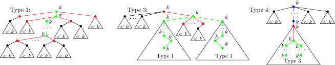
Figure 6: The path $P$ in green for the proof of Theorem 4.2.

5 Conclusion

We have given an $O(n\log n)$ algorithm computing the LMIM-width and an optimal layout of an $n$-node tree. This is the first graph class of LMIM-width larger than $1$ having a polynomial-time algorithm computing LMIM-width and thus constitutes an important step towards a better understanding of LMIM-width. Indeed, for the development of FPT algorithms computing tree-width and path-width of general graphs, one could argue that the algorithm of [7] computing optimal path-decompositions of a tree in time $O(n\log n)$ was a stepping stone. The situation is different for MIM-width and LMIM-width, as it is W-hard to compute these parameters [19], but it is similar in the sense that our objective has been to achieve an understanding of how to take a graph and assemble a decomposition of it, in this case a linear one, such that it has cuts of low MIM. To achieve this objective a polynomial-time algorithm for trees has been our main goal.

References

- [1] Isolde Adler and Mamadou Moustapha Kanté. Linear rank-width and linear clique-width of trees. Theor. Comput. Sci., 589:87–98, 2015.
- [2] Rémy Belmonte and Martin Vatshelle. Graph classes with structured neighborhoods and algorithmic applications. Theor. Comput. Sci., 511:54 – 65, 2013.
- [3] Benjamin Bergougnoux and Mamadou Moustapha Kanté. Rank based approach on graphs with structured neighborhood. CoRR, abs/1805.11275, 2018.
- [4] Hans L. Bodlaender. A linear-time algorithm for finding tree-decompositions of small treewidth. SIAM J. Comput., 25(6):1305–1317, 1996.
- [5] Binh-Minh Bui-Xuan, Jan Arne Telle, and Martin Vatshelle. Fast dynamic programming for locally checkable vertex subset and vertex partitioning problems. Theor. Comput. Sci., 511:66 – 76, 2013.
- [6] Reinhard Diestel. Graph Theory, 4th Edition, volume 173 of Graduate texts in mathematics. Springer, 2012.
- [7] John A. Ellis, Ivan Hal Sudborough, and Jonathan S. Turner. The vertex separation and search number of a graph. Inf. Comput., 113(1):50–79, 1994.
- [8] Fedor V. Fomin, Petr A. Golovach, and Jean-Florent Raymond. On the tractability of optimization problems on H-graphs. In Proc. ESA 2018, pages 30:1 – 30:14, 2018.
- [9] Esther Galby, Andrea Munaro, and Bernard Ries. Semitotal domination: New hardness results and a polynomial-time algorithm for graphs of bounded mim-width. CoRR, abs/1810.06872, 2018.
- [10] Petr A. Golovach, Pinar Heggernes, Mamadou Moustapha Kanté, Dieter Kratsch, Sigve Hortemo Sæther, and Yngve Villanger. Output-polynomial enumeration on graphs of bounded (local) linear mim-width. Algorithmica, 80(2):714–741, 2018.
- [11] Martin Charles Golumbic and Udi Rotics. On the clique-width of some perfect graph classes. Int. J. Found. Comput. Sci., 11(3):423–443, 2000.
- [12] Petr Hlinený, Sang-il Oum, Detlef Seese, and Georg Gottlob. Width parameters beyond tree-width and their applications. Comput. J., 51(3):326–362, 2008.
- [13] Lars Jaffke, O-joung Kwon, Torstein J. F. Strømme, and Jan Arne Telle. Generalized distance domination problems and their complexity on graphs of bounded mim-width. In 13th International Symposium on Parameterized and Exact Computation, IPEC 2018, August 20-24, 2018, Helsinki, Finland, pages 6:1–6:14, 2018.
- [14] Lars Jaffke, O-joung Kwon, and Jan Arne Telle. Polynomial-time algorithms for the longest induced path and induced disjoint paths problems on graphs of bounded mim-width. In 12th International Symposium on Parameterized and Exact Computation, IPEC 2017, September 6-8, 2017, Vienna, Austria, pages 21:1–21:13, 2017.
- [15] Lars Jaffke, O-joung Kwon, and Jan Arne Telle. A unified polynomial-time algorithm for feedback vertex set on graphs of bounded mim-width. In 35th Symposium on Theoretical Aspects of Computer Science, STACS 2018, February 28 to March 3, 2018, Caen, France, pages 42:1–42:14, 2018.
- [16] Stefan Mengel. Lower bounds on the mim-width of some graph classes. Discrete Applied Mathematics, 248:28–32, 2018.
- [17] Rolf H Möhring. Graph problems related to gate matrix layout and pla folding. In Computational graph theory, pages 17–51. Springer, 1990.
- [18] Sang-il Oum. Rank-width: Algorithmic and structural results. Discrete Applied Mathematics, 231:15–24, 2017.
- [19] Sigve Hortemo Sæther and Martin Vatshelle. Hardness of computing width parameters based on branch decompositions over the vertex set. Theor. Comput. Sci., 615:120–125, 2016.
- [20] Martin Vatshelle. New width parameters of graphs. PhD thesis, University of Bergen, Norway, 2012.
- [21] Koichi Yamazaki. Inapproximability of rank, clique, boolean, and maximum induced matching-widths under small set expansion hypothesis. Algorithms, 11(11):173, 2018.