Electron-Extraction from Excited Quantum Dots with Higher Order Coulomb Scattering

Abstract

The electron kinetics in nanowire-based hot-carrier solar cells is studied, where both relaxation and extraction are considered concurrently. Our kinetics is formulated in the many-particle basis of the interacting system. Detailed comparison with simplified calculations based on product states shows that this includes the Coulomb interaction both in lowest and higher orders. While relaxation rates of 1 ps are obtained, if lowest order processes are available, timescales of tens of ps arise if these are not allowed for particular designs and initial conditions. Based on these calculations we quantify the second order effects and discuss the extraction efficiency, which remains low unless an energy filter by resonant tunnelling is applied.

Keywords: Hot-Carrier Solar Cells, Quantum Kinetics, Thermalisation.

1 Introduction

The solar spectrum covers a wide range of energies. In contrast, for an optoelectronic device, we only achieve a good efficiency by adding electrons or holes at the respective electrochemical potential of the contacts [1, 2]. Thus, only a defined exciton energy is efficiently converted to electrical energy. This is the origin of the ultimate efficiency limit of Shockley and Queisser [3].

The idea both behind hot-carrier solar cells [4, 5, 6] or Multiple Exciton Generation (MEG) devices [7, 8, 9, 10, 11] is to combine different excitonic energies to the optimal one by employing the inter-particle Coulomb interaction and extract those at the corresponding difference of electrochemical potentials. The conversion efficiency of hot-carrier solar cells has been extensively studied under different conditions [12, 13, 14, 2, 15]. A big contribution to conversion loss in a hot-carrier solar cell is the thermalisation between the hot electron and the lattice, an objective is thus to increase the thermalisation time in the cell [16, 17, 18, 19]. Further, it has been argued that the hot-carrier cooling rate can be slowed down by a combination of phonon bottleneck [20] and reduced accessibility of the phase space by employing nanostructures like quantum wells or quantum dots (QDs) rather than their bulk counterpart [21, 22, 23, 24, 25]. Note that in addition to the extended hot-carrier cooling time, nanowire heterostructure solar cells also exhibit tunable photoabsorption beyond that of the bulk analogue [26, 27, 28, 29, 30, 31].

A source of the slowed cooling rate in low dimensional nanostructures is the quantization effect from confinement of the electronic wave function, which affects the possibility of Auger processes between the carriers [9, 32]. The Auger process is in turn mediated by the Coulomb interaction which must be included when modelling carrier dynamics. Studies on carrier dynamics after MEG have employed master equations which include the Coulomb interaction to first order [33, 34]. Here we seek to describe the solar cell using a master equation approach that includes the Coulomb interaction to higher orders.

In order to efficiently employ these hot-carrier schemes energetically narrow filters must be implemented which allow for selective extraction of excitons [14, 35, 36, 37]. The hot-carrier solar cell thus requires an appropriate kinetics and properly matched extraction processes, which we study in detail in this article. Here we only concentrate on the electronic part, assuming that the holes are generated at the top of the valence band and are collected from there.

Following the discussion above, we divide our study in three parts: At first we consider the kinetics of electrons after photoexcitation with a high photon energy, where we study the rate of formation of multiple excited electrons after an initial high energy excitation. This process is dominated by the electron-electron interaction and we show that both first-order scattering processes and higher-order contributions play an important role. At second we discuss the features of the extraction kinetics through a single barrier and show that for a system dominated by second order transitions the extraction kinetics is impaired compared to first order. Finally we show how to amend the impairment by implementing a narrow energy filter, i.e. changing the barrier geometry to a double barrier potential.

2 Methods and Model

To study the extraction kinetics in the nanowire QD we need to time-evolve the electronic quantum states in the presence of Coulomb interactions, relaxation processes, and tunnelling to electron reservoir regions. For this purpose we first determine the single-particle states of the electrons in the QD and evaluate the Coulomb interaction between these. For the electronic eigenstates of the interacting system we consider time-evolution of density matrix within the Lindblad master equation [38], where dephasing and extraction is treated via the PERLind approach [39].

2.1 Geometry and Single-Particle Levels

The InAs/InP nanowire axial heterostructure constitutes an interesting system for the solar energy conversion in nanostructures[40]. We model the QD as an InAs cylinder with height $L=$8\text{\,}\mathrm{nm}$$ and radius $R=$8\text{\,}\mathrm{nm}$$ between InP barriers forming a finite well in the conduction band, see Figure 1. A similar system has been realised and shown to function as a hot-carrier solar cell [40, 41]. While the dimensions are chosen slightly smaller than typical structures, this yields a model system for which the calculation of the many-particle eigen-states is tractable. Likewise, we restrict our model to include only the electrons in the conduction band, and thus exclude valence band holes, for the sake of computational complexity. We assume that the conduction band discontinuity between InAs and InP in a thin nanowire provides a potential well of depth $V_{0}=$0.7\text{\,}\rme\mathrm{V}$$, which is of the same order of magnitude as the observed discontinuity [42, 43, 44]. Finally, the effective masses are $m_{\mathrm{InAs}}=0.023m_{e}$ [45] and $m_{\mathrm{InP}}=0.073m_{e}$ [46], where $m_{e}$ is the free electron mass.

To consider extraction we connect one side of the QD to a collecting contact region with potential offset $\varrho$ which prohibits electrons with energy lower than this level to be extracted from the QD, see Figure 1. This can be achieved using a ternary alloy. We model this region as a semiconductor with a conduction band minimum at $\varrho$ and apply the effective mass of InAs, for simplicity.

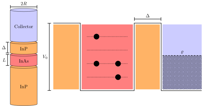
Figure 1: Geometry (left) and energy (right) schematics of the nanowire QD system. The QD is assumed to be a cylindrical piece of InAs with height $L$ and radius $R$. To the one side it is connected to a collecting contact region after an InP barrier of length $\Delta$.

The single-particle levels provided in Figure 2 are evaluated using heterostructure envelope functions in the effective mass approximation [47]. Integrating the density of the electronic envelope function over the volume contained within a shell of $1\text{\,}\mathrm{n}\mathrm{m}$ thickness around the quantum dot we obtain norms above 0.95 for all states – more than 95 percent of the electronic wavefunction is contained within the shell. This allows us to consider geometries with barriers as thin as $\Delta=$1\text{\,}\mathrm{nm}$$ while still applying a basis of confinement states calculated for infinitely thick barriers.

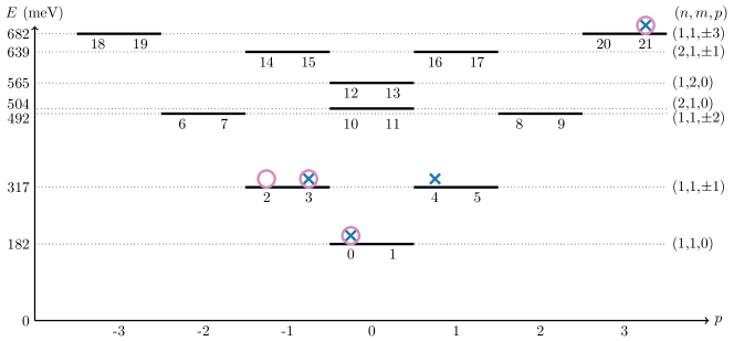
Figure 2: Single-particle levels for the cylindrical InAs QD with height $L=$8\text{\,}\mathrm{nm}$$ and radius $R=$8\text{\,}\mathrm{nm}$$. Every solid line represents a confinement orbital, even numbered states have spin up and odd spin down. The quantum numbers $(n,m,p)$ describe the axial, radial and angular quantization respectively. The blue crosses and violet circles represent the initial states $\left|A\right\rangle=\left|0,3,4,21\right\rangle$ and $\left|B\right\rangle=\left|0,2,3,21\right\rangle$ respectively, which we will consider in Sec. 3.

2.2 Coulomb Matrix Elements

An important part of the electron kinetics in the QD stems from the Coulomb electron-electron interaction, which strongly depends on the spatial overlap of the envelope functions. The general Coulomb matrix is defined in the occupation number representation as

$$\hat{H}_{ee} =\sum_{m<n,l<k}V^{\mathrm{eff}}_{mnkl}\hat{a}^{\dagger}_{m}\hat{a}^{\dagger}_{n}\hat{a}_{k}\hat{a}_{l},$$ (1)

$$V_{mnkl}^{\mathrm{eff}} =V_{mnkl}-V_{mnlk}$$ (2)

Here the $\hat{a}_{i}$ are the annihilation operators for electrons in state $i$ and the Coulomb elements are defined

$$V_{mnkl}=\left\langle\chi_{m}|\chi_{l}\right\rangle\left\langle\chi_{n}|\chi_{k}\right\rangle\frac{e^{2}}{4\pi\varepsilon\varepsilon_{0}}$$

$$\times\int\!\!\!\int\rmd^{3}\mathbf{r}d^{3}\mathbf{r}^{\prime}\varphi^{*}_{m}(\mathbf{r})\varphi_{n}^{*}(\mathbf{r}^{\prime})\frac{1}{|\mathbf{r}-\mathbf{r}^{\prime}|}\varphi_{k}(\mathbf{r}^{\prime})\varphi_{l}(\mathbf{r})$$ (3)

where $\left|\chi\right\rangle$ is the electron’s spin state and $\varphi$ the spatial envelope wave function, $\varepsilon_{0}$ is the vacuum permittivity of free space and $\varepsilon$ the relative permittivity of the material. As the bulk of the electron density is contained within the InAs structure, we use the relative permittivity $\varepsilon_{\mathrm{InAs}}=15$. Further, the considered orbitals all belong to the same band, hence, we can neglect effects resulting from the lattice periodic wave function at the atomic scale. The Coulomb elements are obtained by Monte Carlo integration with importance sampling under the VEGAS routine [48].

Important Coulomb elements are the direct elements and orbital exchange elements, typical values for the two are, respectively,

$$V_{1,3,3,1}=$15\text{\,}\mathrm{m}\mathrm{e}\mathrm{V}$,\qquad V_{1,3,1,3}={$3.8\text{\,}\mathrm{m}\mathrm{e}\mathrm{V}$}.$$ (4)

The size of the direct element can be understood as the charging energy $e^{2}/C$ of a spherical capacitor with capacitance $C=4\pi\epsilon_{0}\varepsilon_{\mathrm{InAs}}r_{\mathrm{eff}}$. Here the energy of $15\text{\,}\mathrm{m}\rme\mathrm{V}$ corresponds to the effective radius $r_{\mathrm{eff}}=$6.2\text{\,}\mathrm{nm}$$. The value of $r_{\mathrm{eff}}$ agrees well with the root mean square distances of the occupation probabilities from the centre of the cylinder, $5.2\text{\,}\mathrm{nm}$ for level 1 and $6.3\text{\,}\mathrm{nm}$ for level 3. The exchange element corresponds to a reduction by a factor of 4 from its respective direct element; this is a typical difference in scale between pairs of direct and exchange elements.

2.3 Density Operator Master Equation

Having determined the electronic single-particle states of the QD we are now in a position to construct the system Hamiltonian and density matrix which we use to perform a Lindbladian time evolution of the system.

From the single-particle orbital energies and the Coulomb matrix we can assemble the full system Hamiltonian

$$\hat{H}=\sum_{i}E_{i}\hat{a}^{\dagger}_{i}\hat{a}_{i}+\hat{H}_{ee}.$$ (5)

The state of the system is described by the reduced density operator $\hat{\rho}_{S}$. When considering the density operator we will neglect coherences between different particle numbers, the operator can thus be further reduced to a tensor product,

$$\hat{\rho}_{S}=\hat{\rho}_{0}\otimes\hat{\rho}_{1}\otimes\ldots\otimes\hat{\rho}_{N},$$ (6)

where $\hat{\rho}_{n}$ is the reduced density operator for $n$ particles and $N$ is the highest number of particles in the system.

Following the method used in Refs. [49, 50] we model the time evolution of the density operator during the extraction of electrons using the Lindblad master equation

$$\hbar\frac{\rmd}{\rmd t}\hat{\rho}_{S}=i[\hat{\rho}_{S},\hat{H}]+\sum_{j}^{N_{\mathrm{jump}}}\Gamma_{j}\left[\hat{L}_{j}\hat{\rho}_{S}\hat{L}_{j}^{\dagger}-\frac{1}{2}\left\{\hat{\rho}_{S},\hat{L}_{j}^{\dagger}\hat{L}_{j}\right\}\right]$$ (7)

where $N_{\mathrm{jump}}$ is the number of jump operators $\hat{L}_{j}$ with rates $\Gamma_{j}/\hbar$.

We define the Lindblad jump operators phenomenologically, where we consider spin-conserving dephasing operators on each orbital $\alpha$,

$$\hat{L}^{\alpha}_{\mathrm{deph}}=\hat{a}_{2\alpha}^{\dagger}\hat{a}_{2\alpha}+\hat{a}_{2\alpha+1}^{\dagger}\hat{a}_{2\alpha+1},$$ (8)

and the extraction operator on state $i$,

$$\hat{L}^{i}_{\mathrm{extr}}=\hat{a}_{i}.$$ (9)

which corresponds to electron transfer to the collecting reservoir.

The dephasing strength, $\Gamma_{\mathrm{deph}}=$6\text{\,}\mathrm{m}\rme\mathrm{V}$$, corresponds to a dephasing time of the order of $100\text{\,}\mathrm{fs}$. This is a typical time scale for these kinetic systems [51]. Considering the extraction strengths we interpret the electron as a classical particle moving back and forth in the dot. The axial kinetic energy thus provides the velocity of the particle in axial direction from which an attempt rate is derived [52],

$$\nu_{i}=\frac{1}{L}\sqrt{\frac{E_{i,z}}{2m_{\mathrm{InAs}}}},$$ (10)

where $E_{i,z}$ is the axial kinetic energy of the envelope state $i$. For the two axial states, $n=1,2$, the attempt rates are

$$\nu_{n=1}=$75\text{\,}\mathrm{p}\mathrm{s}^{-1}$,\qquad\nu_{n=2}=$158\text{\,}\mathrm{p}\mathrm{s}^{-1}$.$$ (11)

The extraction strength, or transmission strength, is determined from the attempt rate as

$$\Gamma^{i}_{\mathrm{extr}}=\hbar\nu_{i}$$ (12)

Note that these are not the final jump operators applied in this work. We will further adjust these with the tunnelling probability in the following section where the energetic information is taken into account.

2.4 Position and Energy Resolving Lindblad Approach

The Lindblad jump operators in Equation (8) and Equation (9) do not carry energetic information about the interactions between the system and bath. A scheme to incorporate these aspects is the Position and Energy Resolving Lindblad approach (PERLind) [39]. Let the states $\left|a\right\rangle,\left|b\right\rangle,$ etc. be an eigenbasis of $\hat{H}$ with $E_{a},E_{b},$ etc. as the corresponding eigenenergies. Then we transform the matrix elements of every jump operator under the PERLind scheme according to

$$\left\langle a\right|\widetilde{L}_{j}\left|b\right\rangle=\sqrt{f_{j}(E_{a}-E_{b})}\left\langle a\right|\hat{L}_{j}\left|b\right\rangle.$$ (13)

Where the function $f_{j}(E)$ describes energy dependence of the jump transition $j$, where $E$ is the energy difference between the final and the initial state. This defines new operators $\widetilde{L}_{j}$ which replace the original operators $\hat{L}_{j}$ in the Lindblad master equation.

For the dephasing operator we assume the interaction to stem from coupling to a phonon bath with temperature $T=$300\text{\,}\mathrm{K}$$. Here we use the heuristic function

$$f_{\mathrm{deph}}(E)=\frac{E/k_{B}T}{\exp(E/k_{B}T)-1}\Theta(D_{\mathrm{InP}}-|E|),$$ (14)

which contains the Bose-distribution $f_{\textrm{Bose}}(E)$ for positive energies (absorption of phonons) and $1+f_{\textrm{Bose}}(|E|)$ for negative $E$ (emission of phonons). The factor $|E|/k_{B}T$ reflects the phonon density of states and the energy dependence of the coupling. $f_{\mathrm{deph}}(E)$ is bounded by the Heaviside step function, $\Theta$, to exclude phonons beyond the Debye energy for InP, $D_{\mathrm{InP}}=$37\text{\,}\mathrm{m}\rme\mathrm{V}$$ [53], which is approximately the largest phonon energy available. Note that dephasing under this model can only connect eigenstates that are separated in energy by less than $D_{\mathrm{InP}}$.

For modifying the extraction we model this process as tunnelling in a finite heterostructure. The modifying function is

$$f_{\mathrm{finite}}(E)=\mathcal{T}(-E)\Theta(-E-\varrho)$$ (15)

where $\mathcal{T}(E_{e})$ is the transmission amplitude described by Tsu and Esaki [54]. Note that the electron energy $E_{e}$ is taken from the electronic system in the quantum dot so that its change in energy is $E=-E_{e}$ during the jump process)

3 Results

In order to obtain an understanding of the relaxation and extraction dynamics we consider qualitatively different initial states of the system with singly excited electrons. Specifically, we choose the product states $\left|A\right\rangle=\left|0,3,4,21\right\rangle$ and $\left|B\right\rangle=\left|0,2,3,21\right\rangle$, which we assume to be generated by some single-particle excitation process not specified here. We consider these states to be two representative cases of the span of possible excited carrier states. State $\left|A\right\rangle$ is close in energy with $\left|0,3,8,9\right\rangle$ and $V_{8,9,21,4}=$4.4\text{\,}\mathrm{m}\mathrm{e}\mathrm{V}$$, which results in a fast Auger process. For $\left|B\right\rangle$, the corresponding Coulomb matrix element ${V_{8,9,21,2}=0}$ due to conservation of angular momentum, which should provide a longer lifetime. These states will be used to examine thermalisation processes in the QD and subsequently to consider the extraction kinetics. Here we will treat three different aspects subsequently: (i) the quantum kinetics implied by the electron-electron-interaction, (ii) the thermalisation induced by our choice of energy dependent dephasing, and (iii) the extraction of carriers.

3.1 Quantum beating in the QD

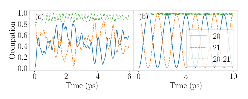
(a)

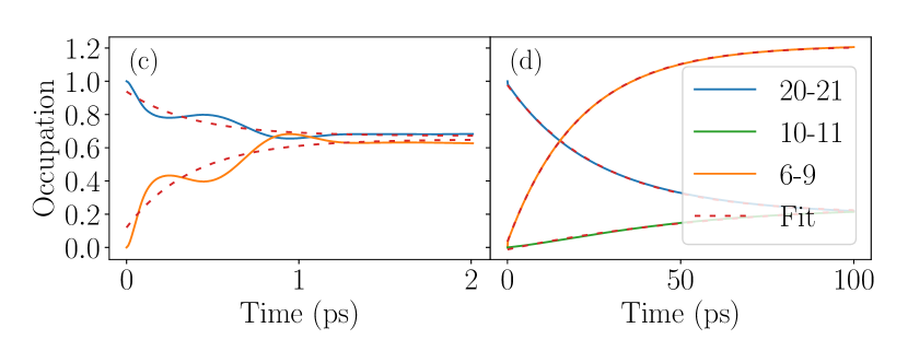
(b)

Figure 3: Time-dependence of occupations of selected single-particle levels as denoted in Fig. 2 for the initial states $\left|A\right\rangle=\left|0,3,4,21\right\rangle$ (left) and $\left|B\right\rangle=\left|0,2,3,21\right\rangle$ (right). In (a) and (b), dephasing and extraction is disregarded and the pure quantum evolution shows distinct quantum beatings, which mainly exchanges the populations of states 20 and 21 (as well as 1 and 0, not shown). Panels (c) and (d) show the corresponding results in the presence of dephasing $\Gamma_{\textrm{deph}}=6$ meV, where we sum the occupations over groups of states strongly coupled by the quantum beating. Here the dashed red lines provide exponential fits to the respective occupations, where we extracted the thermalisation times $0.38\text{\,}\mathrm{p}\mathrm{s}$ for draining of the hot-carrier levels 20-21 (blue) and $0.38\text{\,}\mathrm{p}\mathrm{s}$ for filling of levels 6-9 (orange) during the evolution of $\left|A\right\rangle$ in panel (c). The alternative initial state $\left|B\right\rangle$ in panel (d) provides $26\text{\,}\mathrm{p}\mathrm{s}$ for the draining of hot-carrier levels 20-21, $55\text{\,}\mathrm{p}\mathrm{s}$ for filling of levels 10-11 and $20\text{\,}\mathrm{p}\mathrm{s}$ for levels 6-9.

Figure 3(a,b) shows the evolution of single-particle occupations upon quantum evolution of (7) under the neglect of all jump operators. Here the electron-electron interaction couples the states with each other leading to quantum beating between different states with similar energy. Most importantly, the pair of levels $(0,21)$, which is occupied initially in both cases, is coupled to $(1,20)$ via the matrix element

$$V_{20,1,21,0}=$0.781\text{\,}\mathrm{m}\mathrm{e}\mathrm{V}$,$$ (16)

This results in a beating between both occupations, as can be seen in Figs. 3(a,b) for both initial states. While the occupations of levels 20 and 21 strongly alter in time, their sum remains close to 1. For the initial state $\left|A\right\rangle$ a complex quasi-periodic scenario occurs, see Fig. 3(a), due to a second pair of equivalent levels $(4,21)\leftrightarrow(20,5)$. Additionally, further states are close to resonance here. In contrast, Fig. 3(b) displays an almost ideal beating between the states $\left|B\right\rangle$ and $\left|1,2,3,20\right\rangle$ with the frequency $f^{B}_{\textrm{beat}}=0.49$ THz. Surprisingly, $f^{B}_{\textrm{beat}}$ differs from $2V_{20,1,21,0}/h\approx 0.38$ THz, which we expect from the direct interaction between these states. This difference can be attributed to higher orders in the electron-electron interaction. Actually, the observed frequency can be well reproduced by taking into account the second order terms[55] in the effective matrix element between the beating states:

$$\left\langle 1,2,3,20\right|\hat{H}^{(2)}\left|0,2,3,21\right\rangle$$

$$= V_{20,1,21,0}+\sum_{\left|m\right\rangle}\frac{\left\langle 1,2,3,20\right|\hat{H}\left|m\right\rangle\left\langle m\right|\hat{H}\left|0,2,3,21\right\rangle}{E_{\left|0,2,3,21\right\rangle}-E_{\left|m\right\rangle}}$$

$$= $1.1\text{\,}\mathrm{m}\mathrm{e}\mathrm{V}$\approx\frac{h}{2}0.51\textrm{ THz}\,,$$ (17)

where the sum $\left|m\right\rangle$ runs over all different states which connect the initial and final states. This demonstrates the high relevance of second-order couplings for QD systems of typical sizes.

3.2 Relaxation due to dephasing

Upon introducing the dephasing jump operators in (7), we find relaxation processes to different states as the coherent evolution is broken due to the coupling to the environment. In order to obtain signals relevant for extraction of electrons we sum the occupations of levels, for which strong beating effects occur as addressed in subsection 3.1. The results are shown in Fig. 3(c,d) for the initial states $\left|A\right\rangle,\left|B\right\rangle$, respectively.

Assuming that the probability drift can be described as exponential convergence, we are able to extract the thermalisation times of the systems in Figure 3(c,d). For the initial state $\left|A\right\rangle$, see, Figure 3(c), we find that the time scale of draining the hot-carrier levels 20-21 as well as the filling of levels 6-9 occur on the time scale $\tau^{A}_{\mathrm{drain}}=\tau_{\mathrm{fill}}^{A}=$$0.38\text{\,}\mathrm{p}\mathrm{s}$. These time scales are of the same magnitude as recently observed thermalisation and cooling times in highly excited InAs nanowires [56]. The scattering rate of a single Auger process with Coulomb element $V$ and detuning $\Delta E$ is estimated using Fermi’s golden rule

$$\Lambda=\frac{\left|V\right|^{2}}{\hbar}2\pi\delta_{\widetilde{\Gamma}_{\mathrm{deph}}}(\Delta E)$$ (18)

with Lorentzian broadening

$$2\pi\delta_{\widetilde{\Gamma}_{\mathrm{deph}}}(\Delta E)=\frac{\widetilde{\Gamma}_{\mathrm{deph}}}{\Delta E^{2}+\widetilde{\Gamma}_{\mathrm{deph}}^{2}/4}.$$ (19)

where we employ the dephasing strength

$$\widetilde{\Gamma}_{\mathrm{deph}}=\Gamma_{\mathrm{deph}}f_{\mathrm{deph}}(\Delta E).$$ (20)

(The energy-dependence on $\Gamma_{\mathrm{deph}}$ is not strictly compatible with the use of a Lorentzian. However, we refrain from a more elaborate description here.)

To estimate the effective scattering rates, we consider a subset of the Hilbert space and have to take into account the multiplicities of the relevant initial and final states, between which strong beatings occur as discussed above. The initial state has to be treated as $N_{i}=6$ degenerate product states, which are accessible by Coulomb matrix elements, while the final states (with two of the levels 6-9 occupied) has $N_{f}=2$. Furthermore, as two of the initial product states do not connect to the final states there are $N_{p}=4$ possible Auger processes between them with rate $\Lambda^{A}_{i\to f}$. Straightforward algebra provides

$$\frac{1}{t_{\mathrm{drain}}^{A}}=\Lambda^{A}_{i\to f}\frac{N_{p}}{N_{i}}+\Lambda^{A}_{i\to f}e^{(E_{f}-E_{i})/k_{B}T}\frac{N_{p}}{N_{f}}$$ (21)

where the backward process satisfying detailed balance was also taken into account. With $E_{f}-E_{i}=$13.5\text{\,}\mathrm{m}\mathrm{e}\mathrm{V}$$, Fermi’s golden rule provides $\Lambda^{A}_{i\to f}=$1.45\text{\,}\mathrm{p}\mathrm{s}^{-1}$$, which yields a drain time of $t^{A}_{\mathrm{drain}}=$0.46\text{\,}\mathrm{p}\mathrm{s}$$. This agrees reasonably well with the fitted time scale above. The discrepancy of $0.08\text{\,}\mathrm{p}\mathrm{s}$ may be attributed to the thermalisation being on a time scale similar to the beating between the different product states, which is not included in the rate description of Equation (21).

Proceeding to the second initial state, $\left|B\right\rangle$, see Figure 3(d), we find that the fitted time-scale of draining of the hot-carrier levels 20-21 is $\tau_{\mathrm{drain}}^{B}=$26\text{\,}\mathrm{p}\mathrm{s}$$, and levels 6-9 and 10-11 are filled in the time scales $\tau^{B}_{\mathrm{fill1}}=$20\text{\,}\mathrm{p}\mathrm{s}$$ and $\tau^{B}_{\mathrm{fill2}}=$55\text{\,}\mathrm{p}\mathrm{s}$$ respectively. In contrast to state $\left|A\right\rangle$, level 4 is not occupied in $\left|B\right\rangle$. Consequently, the observed draining and filling time scales are much longer, as the most relevant Coulomb scattering via $V_{8,9,21,4}$ for $\left|A\right\rangle$ is not possible for state $\left|B\right\rangle$. Related decay paths to the states $|2,3,4,9\rangle$ or $|0,1,6,21\rangle$, are provided by the elements $V_{4,9,21,0}$ or $V_{1,6,2,3}$, respectively. The energy detuning of these are $\Delta E=$-54\text{\,}\mathrm{m}\mathrm{e}\mathrm{V}$$ and $\Delta E=$43\text{\,}\mathrm{m}\mathrm{e}\mathrm{V}$$ (including charging energy), respectively, which surpass the energy cut-off $D_{\textrm{InP}}=$37\text{\,}\mathrm{m}\mathrm{e}\mathrm{V}$$. Hence, these transitions are not individually accessible. Yet, by combining both channels in a second order transition we obtain a total detuning of $\Delta E=$-14\text{\,}\mathrm{m}\mathrm{e}\mathrm{V}$$, well within the allowed range. Other decay paths carry the same pattern of being excluded separately yet allowed in combination due to the detuning considerations. Hence, from our model assumptions, first order transitions are forbidden in this thermalisation process, yet second order and higher combinations of these are allowed.

Similarly to Sec. 3.1, the second order transition rate from the initial state $\left|i\right\rangle$ to a final state $\left|f\right\rangle$ over states $\left|m\right\rangle$ is calculated according to second order perturbation theory

$$\Lambda^{\mathrm{B}}_{i\rightarrow f}=\sum_{\left|m\right\rangle}\left|\frac{\left\langle f\right|\hat{H}\left|m\right\rangle\left\langle m\right|\hat{H}\left|i\right\rangle}{E_{i}-E_{m}}\right|^{2}\frac{2\pi}{\hbar}\delta_{{\widetilde{\Gamma}}_{\mathrm{deph}}}(E_{f}-E_{i}).$$ (22)

Due to the $E_{i}-E_{m}$ term in the numerator above we cannot in general use the Boltzmann term $e^{(E_{f}-E_{i})/k_{B}T}$ to convert between the rates for opposite directions.

Following the same procedure as for system A we consider a subset of the Hilbert space with multiplicities $N_{i}=2$ for the initial set of states with one electron in levels 20-21 and $N_{f}=2$ for the set of final states $\{\left|1,4,6,9\right\rangle,\left|0,5,7,8\right\rangle\}$ which are also the spin mirror of each other. There are $N_{p}=4$ Auger processes connecting the two sets, however, unlike for system $A$ the individual processes vary in strength. The full rate is thus

$$\frac{1}{t_{\mathrm{drain}}^{B}}=\sum_{i,f}\left(\frac{\Lambda^{B}_{i\rightarrow f}}{N_{i}}+\frac{\Lambda^{B}_{f\rightarrow i}}{N_{f}}\right)$$ (23)

Summing over all possible transition channels we obtain the drain time $t_{\mathrm{drain}}^{B}=$43\text{\,}\mathrm{p}\mathrm{s}$$. This is larger than the times observed on Fig. 3(d). This discrepancy may be attributed to the presence of four other states with two electrons in levels 6-9 which compete for the occupation from the initial states. The transition rates for these states and our subset have the same order of magnitude and thus contribute to draining the initial state on a relevant time scale. Hence, our subsystem reaches the thermalised distribution quicker than our estimate which considers the subsystem in isolation.

Note that Equation (22) assumes an incoherent addition of the different contributions to the same final state. If we rather employ a coherent addition of the rates,

$$\Lambda^{\mathrm{coh.}}_{i\rightarrow f}=\left|\sum_{\left|m\right\rangle}\frac{\left\langle f\right|\hat{H}\left|m\right\rangle\left\langle m\right|\hat{H}\left|i\right\rangle}{E_{i}-E_{m}}\right|^{2}\frac{2\pi}{\hbar}\delta_{{\widetilde{\Gamma}}_{\mathrm{deph}}}(E_{f}-E_{i})$$

one obtains a drain time of $498\text{\,}\mathrm{p}\mathrm{s}$ which deviates by an order of magnitude from the observed draining time. As the dephasing time scale is $\tau_{\mathrm{deph}}\sim\hbar/\Gamma_{\mathrm{deph}}=$0.1\text{\,}\mathrm{p}\mathrm{s}$$ the observed thermalisation is much slower than the dephasing making coherent addition inapplicable. Additionally, coherent transitions are derived under the assumption of unitary time evolution which is not the case for for the Lindblad master equation, further explaining the necessity of incoherent addition.

The absence of first-order Coulomb scattering in the second initial state results in slow thermalisation. This makes us regard it as a worst-case scenario, with respect to quantum efficiency, among possible initial states of the system. As we will see in the subsequent section this renders the quantum efficiency from the second initial state more difficult to augment above unity.

3.3 Extraction through single barrier

Above we found a difference of almost two orders of magnitude in the thermalisation time scales between the two initial states under consideration. We now include extraction operators from Eq. (9) in the Lindbladian time evolution in order to investigate the impact of thermalisation on the extraction processes.

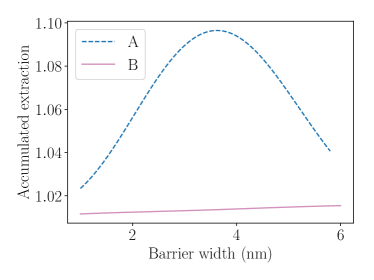
(a)

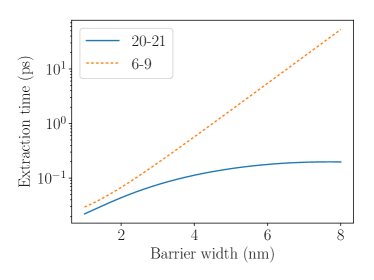
(b)

Figure 4: Left: comparison of extraction from the QD through a single barrier potential in the considered initial states $\left|A\right\rangle$ (dashed blue) and $\left|B\right\rangle$ (solid violet) after $100\text{\,}\mathrm{p}\mathrm{s}$. Right: extraction times for selected levels in $\left|A\right\rangle$ and $\left|B\right\rangle$.

We want to investigate the effect of thermalisation whereby the hot-carrier shares its energy with the three low-energy electrons. Hence, we seek to exclude possible extraction contributions stemming solely from the interaction between these three. A discernible Auger process among the three lower electrons is the decay of the particle in level 3 into 1 which excites the other electron from state 2 to a virtual state of $489\text{\,}\mathrm{m}\rme\mathrm{V}$. To preclude this contribution the potential offset in the nanowire is set to ${\varrho=$500\text{\,}\mathrm{m}\rme\mathrm{V}$}$. Thus, no single electron from the initial states $\left|A\right\rangle$, $\left|B\right\rangle$ can escape from the QD unless the excited electron in level 21 participates.

Figure 4(left) shows the accumulated particle extraction for different barrier widths for both initial conditions. Considering the initial state $\left|A\right\rangle$, dashed blue, we find that the accumulated extraction has an optimum at a barrier width of $3.6\text{\,}\mathrm{n}\mathrm{m}$ with an electron extraction more than 0.09 above unity. In order to understand the position of the optimum we consider the extraction times of the selected orbitals, see Figure 4(right). At a barrier width around $1\text{\,}\mathrm{n}\mathrm{m}$ the extraction time is around $0.02\text{\,}\mathrm{ps}$ for the upper levels 20-21. This is three orders of magnitude smaller than the system thermalisation time and thus the hot-carrier does not have sufficient time to share a significant amount of its energy with the other electrons before it is extracted. Hence, we have only a small increase of electron extraction above unity.

As the barrier width is increased the extraction time of the high energy electron, solid blue curve, increases. From the WKB approximation the time increases approximately exponentially [57],

$$\tau\sim T(E_{e})^{-1}\sim\rme^{\kappa\Delta},\quad\kappa=\sqrt{2{m_{\mathrm{InP}}}(V_{0}-E_{e})}.$$ (24)

with parameters defined in sec. 2.1 and 2.4. This enables the hot-carrier to share more of its energy with the other electrons, thus increasing the accumulated extraction. However, from the WKB approximation we also see that the extraction time is essentially dependent on the decay parameter $\kappa$, which is smaller for electrons with higher energy. Thus the extraction time for the levels 6-9, dashed orange, increase quicker than that of the hot-carrier, which hinders the efficient extraction from these states before the carrier is extracted from the QD. If the levels 6-9 are emptied much slower than levels 20-21 the rate equations from the previous subsection show that occupation flows back into the hot-carrier levels, reducing the quantum efficiency. These two opposing concerns appear to balance out just below a barrier width of $4\text{\,}\mathrm{n}\mathrm{m}$.

We now turn to the initial state $\left|B\right\rangle$, the total extraction after $100\text{\,}\mathrm{p}\mathrm{s}$ is provided in Figure 4(left). We find that the extraction never yields more than 0.02 above unity. According to Figure 4(right) the extraction time of the hot-carrier levels 20-21 never exceeds $1\text{\,}\mathrm{p}\mathrm{s}$ within the barrier widths of interest, which is an order of magnitude faster than the thermalisation time for this initial state, see the previous subsection. While our model provides larger extraction rates for barrier widths exceeding $6\text{\,}\mathrm{n}\mathrm{m}$ and longer collection times, such results should not be taken too seriously. For time scales approaching 100 ps, further interaction processes, not included here, become of relevance for the thermalisation and will eventually limit the extraction. Examples could be multiple-phonon interaction or remote scattering with plasmons in gate contacts.

3.4 Extraction through double barrier

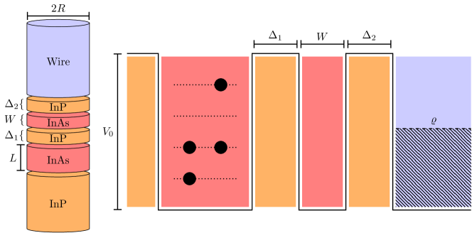
Figure 5: Geometry and energy schematics of the nanowire QD system with double barrier heterostructure. The QD is assumed to be a cylindrical piece of InAs with height $L$ and radius $R$. To the one side it is connected to a thick barrier of InP and to the other a superlattice structure of cylindrical segments; an InP barrier of width $\Delta_{1}$, InAs well region of width $W$ and then another InP barrier of width $\Delta_{2}$, before it reaches the nanowire.

We have identified the slow thermalisation of the initial state $\left|B\right\rangle$ to impair the total extraction through a single barrier due to significant leaking of the hot-carrier. Now we tailor the extraction region to improve the extraction from the levels 6-11, while disfavouring extraction from the initially occupied state 21. This can be achieved by creating a double barrier region and adjusting the widths according to resonant tunnelling for levels 6-11, see Figure 5.

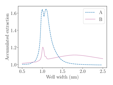
(a)

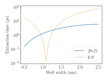
(b)

Figure 6: Extraction through a double barrier heterostructure from QD into nanowire with barrier widths $\Delta_{1}=\Delta_{2}=$4\text{\,}\mathrm{n}\mathrm{m}$$ and potential offset in the nanowire $\varrho=$500\text{\,}\mathrm{m}\mathrm{e}\mathrm{V}$$. Left: Extraction after $100\text{\,}\mathrm{ps}$ for varying well widths. Right: Extraction times in $\left|A\right\rangle$ and $\left|B\right\rangle$ for selected levels for different well widths.

We let both barrier widths be $\Delta_{1}=\Delta_{2}=$4\text{\,}\mathrm{nm}$$ and vary the length of the of the well, $W$, between the two barriers, see Figure 6 (left). The initial state is $\left|B\right\rangle$ and we simulate the initial $100\text{\,}\mathrm{ps}$. From the accumulated extraction we see, for widths between 1 and $2\text{\,}\mathrm{nm}$, a considerable increase in extracted electrons compared to the single barrier extraction, cf. Figure 4(b), with the tallest peak at $W=$1\text{\,}\mathrm{nm}$$ where the extraction is 1.2 electrons. If we consider the extraction times for selected levels, Figure 6 (right), we find that the extraction time of the high energy levels, solid blue curve, is monotonically increasing; above a width of $1\text{\,}\mathrm{nm}$ it is larger than $2\text{\,}\mathrm{ps}$ and thus within an order of magnitude of the thermalisation time. Additionally, the extraction times of the orbitals close to $500\text{\,}\mathrm{m}\rme\mathrm{V}$, dashed green and dotted orange, are comparable to or smaller than the thermalisation time in the interval between 1 and $1.7\text{\,}\mathrm{nm}$. Below $1\text{\,}\mathrm{nm}$ the extraction time of the hot-carrier is too small to allow significant redistribution of the energy while above $2\text{\,}\mathrm{nm}$ the extraction times of levels 6-11 are too large to allow significant extraction of these states. The pronounced peak in extraction around $1\text{\,}\mathrm{nm}$ well width is due to the tunnelling resonances for level 6-9 with the ground level in the well. With perfect transmission for equal barriers, the extraction rate approaches $\approx$75\text{\,}\mathrm{ps}$^{-1}$, which provides a level broadening of $50\text{\,}\mathrm{m}\rme\mathrm{V}$. The combined dephasing and extraction broadening at resonance increases the detuning width of $\delta_{\Gamma}(\Delta E)$ which enables a faster relaxation of the hot-carrier compared to pure dephasing. Thus, relaxation and extraction processes cannot be treated separately, if extraction rates become faster than $0.1\text{\,}\mathrm{p}\mathrm{s}$.

Importantly, while the quantum efficiency of the double barrier potential is particularly improved at resonance widths close to $1\text{\,}\mathrm{n}\mathrm{m}$, the overall accumulated extraction is improved for all widths between $1.5\text{\,}\mathrm{n}\mathrm{m}$ and $2\text{\,}\mathrm{n}\mathrm{m}$, more than 0.1 above unity. Even off-resonance the double barrier potential is a useful geometric configuration. Due to the above considerations we expect that quickly thermalisable states will likewise exhibit a pronounced increase in quantum efficiency if we apply a similar double barrier potential. From Fig 6 (left) we find this to be the case for state $\left|A\right\rangle$ with a broad peak reaching extractions of 0.6 above unity.

4 Conclusions

The kinetics of photo-excited carriers in a nanowire quantum dot system was studied. We find, that both first and second-order terms in the electron-electron interactions are relevant, which is fully taken into account by our PERLind approach applying a basis of many-particle eigenstates of the quantum dot system. Phenomenological dephasing and tunnelling can be directly included and we find a strong dependence on details of the system, such as the particular excited state. In particular, we quantify the thermalization due to second order processes, where a variety of different paths need to be added incoherently. We also point out, that very efficient extraction can enable further transition processes due to broadening, which is fully taken into account by our approach.

If first-order processes in the electron-electron scattering are energetically disfavoured our model provides rather long thermalisation times as expected. However, even in this situation an increased extraction of electrons can be achieved by including a double-barrier extraction structure. Here the efficiency is not too sensitive to the actual resonance energy, so that fluctuations in the well width of 10 % do not affect the efficiency dramatically and the effect should be observable. For quick thermalisation, when first order processes are possible, even higher total extraction up to 1.6 are found. The extraction above unity means, that the excess energy of the excitation above the band gap due to a high energy photon can be converted into extra current, and constitutes an interesting mechanism for advancing the efficiency of the solar cells [4, 7].

It would be interesting to study these processes experimentally by specifically designed optical pulses to provide specific single highly excited states similar to our states $|A\rangle$ and $|B\rangle$ in such nanowire structures. These experiments can be directly modeled by our approach, if the optical field is explicitly taken into account extending earlier work[50]. In this context it is also interesting to take into account non-ideal nanowire shapes seen in real systems, which, however, requires a substantially larger numerical effort.

References

- [1] U. Würfel, A. Cuevas, and P. Würfel. Charge carrier separation in solar cells. IEEE Journal of Photovoltaics, 5(1):461–469, Jan 2015.
- [2] S. Limpert, S. Bremner, and H. Linke. Reversible electron-hole separation in a hot carrier solar cell. New J. Phys., 17:095004, 2015.
- [3] William Shockley and Hans J. Queisser. Detailed balance limit of efficiency of p-n junction solar cells. J. Appl. Phys., 32(3):510–519, 1961.
- [4] Robert T. Ross and Arthur J. Nozik. Efficiency of hot‐carrier solar energy converters. Journal of Applied Physics, 53(5):3813–3818, 1982.
- [5] Martin A. Green. Third generation photovoltaics: Ultra-high conversion efficiency at low cost. Progress in Photovoltaics: Research and Applications, 9(2):123–135, 2001.
- [6] P. Würfel, A. S. Brown, T. E. Humphrey, and M. A. Green. Particle conservation in the hot-carrier solar cell. Progress in Photovoltaics: Research and Applications, 13(4):277–285, 2005.
- [7] Sabine Kolodinski, Jürgen H. Werner, Thomas Wittchen, and Hans J. Queisser. Quantum efficiencies exceeding unity due to impact ionization in silicon solar cells. Appl. Phys. Lett., 63:2405, 1993.
- [8] P.T. Landsberg, H. Nussbaumer, and G. Willeke. Band‐band impact ionization and solar cell efficiency. J. Appl. Phys., 74:1451, 1993.
- [9] AJ Nozik. Quantum dot solar cells. Physica E, 14(1):115–120, 2002.
- [10] Heather Goodwin, Tom C. Jellicoe, Nathaniel J.L.K. Davis, and Marcus L. Böhm. Multiple exciton generation in quantum dot-based solar cells. Nanophotonics, 1:111–126, 2017.
- [11] Yong Yan, Ryan W. Crisp, Jing Gu, Boris Chernomordik, Gregory F. Pach, Marshall Ashley R., John A. Turner, and Matthew C. Beard. Multiple exciton generation for photoelectrochemical hydrogen evolution reactions with quantum yields exceeding 100%. Nature Energy, 2(17052), 2017.
- [12] P. Aliberti, Y. Feng, Y. Takeda, S. K. Shrestha, M. A. Green, and G. Conibeer. Investigation of theoretical efficiency limit of hot carriers solar cells with a bulk indium nitride absorber. Journal of Applied Physics, 108(9):094507, 2010.
- [13] Yasuhiko Takeda, Tadashi Ito, Tomoyoshi Motohiro, Dirk König, Santosh Shrestha, and Gavin Conibeer. Hot carrier solar cells operating under practical conditions. Journal of Applied Physics, 105(7):074905, 2009.
- [14] Y. Feng, P. Aliberti, B. P. Veettil, R. Patterson, S. Shrestha, M. A. Green, and G. Conibeer. Non-ideal energy selective contacts and their effect on the performance of a hot carrier solar cell with an indium nitride absorber. Applied Physics Letters, 100(5):053502, 2012.
- [15] Simon Kahmann and Maria A. Loi. Hot carrier solar cells and the potential of perovskites for breaking the shockley–queisser limit. J. Mater. Chem. C, 7:2471–2486, 2019.
- [16] Yasuhiko Takeda, Tomoyoshi Motohiro, Dirk König, Pasquale Aliberti, Yu Feng, Santosh Shrestha, and Gavin Conibeer. Practical factors lowering conversion efficiency of hot carrier solar cells. Applied Physics Express, 3(10):104301, oct 2010.
- [17] A. Le Bris and J.-F. Guillemoles. Hot carrier solar cells: Achievable efficiency accounting for heat losses in the absorber and through contacts. Applied Physics Letters, 97(11):113506, 2010.
- [18] Antonio Luque and Antonio Martí. Electron–phonon energy transfer in hot-carrier solar cells. Solar Energy Materials and Solar Cells, 94(2):287 – 296, 2010.
- [19] Chin-Yi Tsai. Theoretical model and simulation of carrier heating with effects of nonequilibrium hot phonons in semiconductor photovoltaic devices. Progress in Photovoltaics: Research and Applications, 26(10):808–824, 2018.
- [20] U Bockelmann and G Bastard. Phonon scattering and energy relaxation in two-, one-, and zero-dimensional electron gases. Physical Review B, 42(14):8947, 1990.
- [21] W. S. Pelouch, R. J. Ellingson, P. E. Powers, C. L. Tang, D. M. Szmyd, and A. J. Nozik. Comparison of hot-carrier relaxation in quantum wells and bulk GaAs at high carrier densities. Phys. Rev. B, 45:1450–1453, Jan 1992.
- [22] Y. Rosenwaks, M. C. Hanna, D. H. Levi, D. M. Szmyd, R. K. Ahrenkiel, and A. J. Nozik. Hot-carrier cooling in GaAs: Quantum wells versus bulk. Phys. Rev. B, 48:14675–14678, Nov 1993.
- [23] Gavin Conibeer, Santosh Shrestha, Shujuan Huang, Robert Patterson, Hongze Xia, Yu Feng, Pengfei Zhang, Neeti Gupta, Murad Tayebjee, Suntrana Smyth, Yuanxun Liao, Shu Lin, Pei Wang, Xi Dai, and Simon Chung. Hot carrier solar cell absorber prerequisites and candidate material systems. Solar Energy Materials and Solar Cells, 135:124 – 129, 2015. EMRS 2014 Spring Meeting – Advanced materials and characterization techniques for solar cells II.
- [24] Gavin Conibeer, Yi Zhang, Stephen P. Bremner, and Santosh Shrestha. Towards an understanding of hot carrier cooling mechanisms in multiple quantum wells. Japanese Journal of Applied Physics, 56(9):091201, jul 2017.
- [25] Dac-Trung Nguyen, Laurent Lombez, François Gibelli, Soline Boyer-Richard, Alain Le Corre, Olivier Durand, and Jean-François Guillemoles. Quantitative experimental assessment of hot carrier-enhanced solar cells at room temperature. Nature Energy, 2:236–242, March 2018.
- [26] Linyou Cao, Justin S. White, Joon-Shik Park, Jon A. Schuller, Bruce M. Clemens, and Mark L. Brongersma. Engineering light absorption in semiconductor nanowire devices. Nature Materials, 8:643–647, 2009.
- [27] Linyou Cao, Pengyu Fan, Alok P. Vasudev, Justin S. White, Zongfu Yu, Wenshan Cai, Jon A. Schuller, Shanhui Fan, and Mark L. Brongersma. Semiconductor nanowire optical antenna solar absorbers. Nano Letters, 10(2):439–445, 2010. PMID: 20078065.
- [28] Phillip M. Wu, Nicklas Anttu, H. Q. Xu, Lars Samuelson, and Mats-Erik Pistol. Colorful InAs nanowire arrays: From strong to weak absorption with geometrical tuning. Nano Letters, 12(4):1990–1995, 2012. PMID: 22409436.
- [29] Sun-Kyung Kim, Robert W. Day, James F. Cahoon, Thomas J. Kempa, Kyung-Deok Song, Hong-Gyu Park, and Charles M. Lieber. Tuning light absorption in core/shell silicon nanowire photovoltaic devices through morphological design. Nano Letters, 12(9):4971–4976, 2012. PMID: 22889329.
- [30] Johannes Svensson, Nicklas Anttu, Neimantas Vainorius, B. Mattias Borg, and Lars-Erik Wernersson. Diameter-dependent photocurrent in InAsSb nanowire infrared photodetectors. Nano Letters, 13(4):1380–1385, 2013. PMID: 23464650.
- [31] Mark L. Brongersma, Yi Cui, and Shanhui Fan. Light management for photovoltaics using high-index nanostructures. Nature Materials, 13:451–460, 2014.
- [32] Matthew C. Beard, Kelly P. Knutsen, Pingrong Yu, Joseph M. Luther, Qing Song, Wyatt K. Metzger, Randy J. Ellingson, and Arthur J. Nozik. Multiple exciton generation in colloidal silicon nanocrystals. Nano Letters, 7(8):2506–2512, 2007. PMID: 17645368.
- [33] A. Shabaev, Al. L. Efros, and A. J. Nozik. Multiexciton generation by a single photon in nanocrystals. Nano Letters, 6(12):2856–2863, 2006.
- [34] A. Franceschetti, J. M. An, and A. Zunger. Impact ionization can explain carrier multiplication in pbse quantum dots. Nano Letters, 6(10):2191–2195, 2006. PMID: 17034081.
- [35] Peter Würfel. Solar energy conversion with hot electrons from impact ionisation. Solar Energy Materials and Solar Cells, 46(1):43 – 52, 1997.
- [36] P. Aliberti, Y. Feng, S. K. Shrestha, M. A. Green, G. Conibeer, L. W. Tu, P. H. Tseng, and R. Clady. Effects of non-ideal energy selective contacts and experimental carrier cooling rate on the performance of an indium nitride based hot carrier solar cell. Applied Physics Letters, 99(22):223507, 2011.
- [37] Yasuhiko Takeda, Akihisa Ichiki, Yuya Kusano, Noriaki Sugimoto, and Tomoyoshi Motohiro. Resonant tunneling diodes as energy-selective contacts used in hot-carrier solar cells. Journal of Applied Physics, 118(12):124510, 2015.
- [38] G. Lindblad. On the generators of quantum dynamical semigroups. Commun. Math. Phys., 48(2):119–130, jun 1976.
- [39] Gediminas Kiršanskas, Martin Franckié, and Andreas Wacker. Phenomenological position and energy resolving Lindblad approach to quantum kinetics. Phys. Rev. B, 97:035432, Jan 2018.
- [40] Steven Limpert, Adam Burke, I-Ju Chen, Nicklas Anttu, Sebastian Lehmann, Sofia Fahlvik, Stephen Bremner, Gavin Conibeer, Claes Thelander, Mats-Erik Pistol, and Heiner Linke. Bipolar photothermoelectric effect across energy filters in single nanowires. Nano Letters, 17(7):4055–4060, 2017. PMID: 28598628.
- [41] Steven Limpert, Adam Burke, I-Ju Chen, Nicklas Anttu, Sebastian Lehmann, Sofia Fahlvik, Stephen Bremner, Gavin Conibeer, Claes Thelander, Mats-Erik Pistol, and Heiner Linke. Single-nanowire, low-bandgap hot carrier solar cells with tunable open-circuit voltage. Nanotechnology, 28(43), 2017.
- [42] Matthew Zervos and Lou-Fé Feiner. Electronic structure of piezoelectric double-barrier InAs/InP/InAs/InP/InAs (111) nanowires. J. Appl. Phys., 95(1):281–291, 2004.
- [43] M. T. Björk, B. J. Ohlsson, T. Sass, A. I. Persson, C. Thelander, M. H. Magnusson, K. Deppert, L. R. Wallenberg, and L. Samuelson. One-dimensional heterostructures in semiconductor nanowhiskers. Appl. Phys. Lett., 80:1058, 2002.
- [44] M. T. Björk, B. J. Ohlsson, C. Thelander, A. I. Persson, K. Deppert, L. R. Wallenberg, and L. Samuelson. Nanowire resonant tunneling diodes. Appl. Phys. Lett., 81:4458, 2002.
- [45] Włodzimierz Nakwaski. Effective masses of electrons and heavy holes in GaAs, InAs, A1As and their ternary compounds. Physica B: Condensed Matter, 210:1–25, 1995.
- [46] T.S. Moss and A.K. Walton. Measurement of effective mass of electrons in InP by infra-red Faraday effect. Physica, 25(7):1142–1144, 1959.
- [47] D. J. BenDaniel and C. B. Duke. Space-charge effects on electron tunneling. Phys. Rev., 152:683–692, Dec 1966.
- [48] Mark Galassi, Jim Davies, James Theiler, Brian Gough, Gerard Jungman, Patrick Alken, Michael Booth, Fabrice Rossi, and Rhys Ulerich. GNU Scientific Library Reference Manual. 3rd edition, 2018.
- [49] Fikeraddis A. Damtie and Andreas Wacker. Time dependent study of multiple exciton generation in nanocrystal quantum dots. J. Phys.:Conf. Ser., 696(1):012012, 2016.
- [50] Fikeraddis A. Damtie, Khadga J. Karki, Tõnu Pullerits, and Andreas Wacker. Optimization schemes for efficient multiple exciton generation and extraction in colloidal quantum dots. J. Chem. Phys., 145(6):064703, 2016.
- [51] R Jasiak, G Manfredi, P-A Hervieux, and M Haefele. Quantum–classical transition in the electron dynamics of thin metal films. New Journal of Physics, 11(6):063042, jun 2009.
- [52] Peter J. Price. Attempt frequency in tunneling. American Journal of Physics, 66(12):1119–1122, 1998.
- [53] Sadao Adachi. Thermal properties. In Physical Properties of III‐V Semiconductor Compounds, chapter 4, pages 48–62. Wiley-Blackwell, 2005.
- [54] R. Tsu and L. Esaki. Tunneling in a finite superlattice. Appl. Phys. Lett., 22(11), june 1973.
- [55] J. J. Sakurai. Modern Quantum Mechanics. Addison Wesley, 1st edition, 1993.
- [56] L. Wittenbecher, J. Vogelsang, S. Lehmann, K. D. Thelander, D. Zigmantas, and A. Mikkelsen. Ultrafast hot electron dynamics in inas nanowires with variable crystal phases investigated by time-resolved photoelectron emission. presented at the LEEM/PEEM workshop, November 2018, Chongqing, China.
- [57] David J. Griffiths. Introduction to Quantum Mechanics. Pearson Prentice Hall, Upper Saddle River, 2nd edition, 2005.