A note on uniform exponential stability of linear periodic time-varying systems

RobertΒ Vrabel Β©2019 IEEE. Personal use of this material is permitted. Permission from IEEE must be obtained for all other uses, in any current or future media, including reprinting/republishing this material for advertising or promotional purposes, creating new collective works, for resale or redistribution to servers or lists, or reuse of any copyrighted component of this work in other works.Digital Object Identifier 10.1109/TAC.2019.2927949
Abstract

In this paper we derive new criterion for uniform stability assessment of the linear periodic time-varying systems $\bm{\dot{x}=A(t)x,$\ $A(t+T)=A(t).}$ As a corollary, the lower and upper bounds for the Floquet characteristic exponents are established. The approach is based on the use of logarithmic norm of the system matrix $\bm{A(t).}$ Finally we analyze the robustness of the stability property under external disturbance.

Index Terms:
Linear periodic time-varying system, uniform exponential stability, uniform stability, logarithmic norm.

I Theory about general linear time-varying systems

I-A Introduction

Stability analysis for linear time-varying (LTV) systems is of constant interest in the control community. One reason is the growing importance of adaptive controllers for which underlying closed-loop adaptive system is time-varying and linear [12, 17, 22]. The second one is that the LTV systems naturally arise when one linearizes nonlinear systems about a non constant nominal trajectory. In contrast the linear time-invariant (LTI) cases which have been thoroughly understood in the analysis and synthesis, many properties of the LTV systems are still not completely resolved. In this context, the system stability analysis can serve as an appropriate example.

The stability characteristics of a linear time-invariant (LTI) system of ordinary differential equations $\dot{x}=Ax$ can be characterized completely by the placement of the eigenvalues of the system matrix $A.$ For systems described by

$$\dot{x}=A(t)x,\quad t\geq t_{0}\,(\geq 0),$$ (1)

one would intuitively expect that if, for each $t,$ the frozen-time system is stable of any kind, then the time-varying system should also be stable provided $A(t)$ is bounded. However these conditions are still not strong enough to guarantee the uniform exponential stability (ExampleΒ 1) and additional restrictions suitably constraining the rate of variation in $A(t)$ have to be imposed. The best known results were given by C.Β A.Β Desoer [9], W.Β A.Β Coppel [6] and H.Β H.Β Rosenbrock [19] in their studies of slowly varying systems. The results are summarized and slightly strengthened in [16, TheoremΒ 3.2]. For illustration purpose, in the following theorem we present two criteria; for some other frozen-time methods for LTV systems see also e.Β g.[18].

Theorem 1

Suppose that $A(t)$ is (piecewise) continuous matrix function $A(\cdot):[0,\infty)\to\mathbb{R}^{n\times n}$ which satisfies:

  • i)

    there exists $M>0$ such that $\left\lVert A(t)\right\rVert<M$ for all $t\geq 0,$

  • ii)

    there exists $\alpha>0$ such that the spectrum

    $\sigma_{A(t)}\subset\left\{z\in\mathbb{C};\,\Re\{z\}<-\alpha\right\}$ for all $t\geq 0.$

Then any of the following conditions guarantees uniform exponential stability of (1):

  • C1)

    $\alpha>4M$ for all $t\geq 0;$

  • C2)

    $A(\cdot)$ is piecewise differentiable and

    $$\left\lVert\dot{A}(t)\right\rVert<\frac{2}{2n-1}\frac{\alpha^{4n-2}}{2M^{4n-4}}\ \mathrm{for\ all}\ t\geq 0.$$
Example 1

For the linear state equation (1) with

$$A_{\beta}(t)=\left[\begin{array}[]{cc}-1+\beta\cos^{2}t&1-\beta\sin t\cos t\\ -1-\beta\sin t\cos t&-1+\beta\sin^{2}t\end{array}\right],\ t\geq 0,$$

where $\beta$ is a positive constant, the pointwise eigenvalues are constants, given by $\sigma_{A_{\beta}(t)}=\frac{1}{2}\left({\beta-2\pm\sqrt{\beta^{2}-4}}\right).$ It is not difficult to verify that the fundamental matrix

$$\Phi_{\beta}(t,0)=\left[\begin{array}[]{cc}e^{(\beta-1)t}\cos t&e^{-t}\sin t\\ -e^{(\beta-1)t}\sin t&e^{-t}\cos t\end{array}\right].$$

Thus while the pointwise eigenvalues of $A_{\beta}(t)$ have negative real parts if $0<\beta<2,$ the state equation has unbounded solutions if $\beta>1,$ [20]. Now if we set $\beta=1.5$ and $t=t^{*}=\pi/2,$ we get $\left\lVert A_{\beta}(t^{*})\right\rVert_{2}=1.7808,$ $\left\lVert\dot{A}_{\beta}(t^{*})\right\rVert_{2}=0.5000,$ $\sigma_{A_{\beta}(t^{*})}=\{-0.2500+0.6614i,\,-0.2500-0.6614i\},$ and so the system does not satisfy neither sufficient condition C1 nor C2. In general, it is difficult to specify exact upper bounds on $\left\lVert A(t)\right\rVert$ and $\left\lVert\dot{A}(t)\right\rVert$ for all $t\geq 0.$

Principally different approach to study of stability of LTV systems is based on the analysis of the small perturbation of the stable nominal system $\dot{x}=A_{\mathrm{nom}}x.$ As is shown in [2] and [7] the perturbed system $\dot{x}=[A_{\mathrm{nom}}+B(t)]x$ preserves the uniform and uniform exponential stability if $\int\limits_{0}^{\infty}\left\lVert B(\tau)\right\rVert d\tau<\infty.$

I-B Notation and definitions

Definition 1 ([3], [7])

Let $X(t)$ is a fundamental matrix solution for (1) and $\Phi(t,\tau)\triangleq X(t)X^{-1}(\tau)$ denotes its corresponding state-transition matrix. Then the system (1) is

  • (US)

    uniformly stable if and only if there exists a positive constant $K$ such that

    $$\left\lVert\Phi(t,\tau)\right\rVert\leq K\ \mathrm{for}\ t_{0}\leq\tau\leq t<\infty,$$
  • (UES)

    uniformly exponentially stable if and only there exist positive constants $K$, $\tilde{\alpha}$ such that

    $$\left\lVert\Phi(t,\tau)\right\rVert\leq Ke^{-\tilde{\alpha}(t-\tau)}\ \mathrm{for}\ t_{0}\leq\tau\leq t<\infty.$$

We will derive results for unspecified vector norm on $\mathbb{R}^{n}$, $\left\lVert\cdot\right\rVert.$ For the matrices, as an operator norm is used the induced norm, $\left\lVert A\right\rVert=\max\limits_{\left\lVert x\right\rVert=1}\left\lVert Ax\right\rVert$. We will use for both vector norm and matrix operator norm the same notation but it will always be clear from the context that norm is being used. In particular cases we will consider the three most common vector norm - $\left\lVert x\right\rVert_{1},$ $\left\lVert x\right\rVert_{2}$ and $\left\lVert x\right\rVert_{\infty}.$ We denote by $\mu[A(t)],$ $t\geq 0,$ the logarithmic norm (LN) of a continuous matrix function $A(t),$ $A(\cdot):[0,\infty)\to\mathbb{R}^{n\times n}$ defined as

$$\mu[A(t)]\triangleq\lim\limits_{h\to 0^{+}}\frac{\left\lVert I_{n}+hA(t)\right\rVert-1}{h},$$

where $I_{n}$ denotes the identity on $\mathbb{R}^{n}$ (see TableΒ I). We note here that the LN $\mu$ is not a norm in the usual sense, because it can take negative values.

TABLE I: Logarithmic norms for the vector norms $\left\lVert\cdot\right\rVert_{1},$ $\left\lVert\cdot\right\rVert_{2}$ and $\left\lVert\cdot\right\rVert_{\infty},$ [1, p.Β 54], [11, p.Β 33].
Vector norm Logarithmic norm
$\left\lVert x\right\rVert_{1}=\sum\limits_{i=1}^{n}|x_{i}|$ ΞΌ1​[A]=max1≀j≀n⁑(aj​j+βˆ‘iβ‰ j|ai​j|)subscriptπœ‡1delimited-[]𝐴subscript1𝑗𝑛subscriptπ‘Žπ‘—π‘—subscript𝑖𝑗subscriptπ‘Žπ‘–π‘—\mu_{1}[A]=\max\limits_{1\leq j\leq n}\left(a_{jj}+\sum\limits_{i\neq j}|a_{ij}|\right)
$\left\lVert x\right\rVert_{2}=\sqrt{\sum\limits_{i=1}^{n}x_{i}^{2}}$ $\mu_{2}[A]=\frac{1}{2}\lambda_{\max}\left({A+A^{T}}\right)$
$\left\lVert x\right\rVert_{\infty}=\max\limits_{1\leq i\leq n}{|x_{i}|}$ ΞΌβˆžβ€‹[A]=max1≀i≀n⁑(ai​i+βˆ‘jβ‰ i|ai​j|)subscriptπœ‡delimited-[]𝐴subscript1𝑖𝑛subscriptπ‘Žπ‘–π‘–subscript𝑗𝑖subscriptπ‘Žπ‘–π‘—\mu_{\infty}[A]=\max\limits_{1\leq i\leq n}\left(a_{ii}+\sum\limits_{j\neq i}|a_{ij}|\right)

In TableΒ I and elsewhere in the paper, the superscript ’T’ denotes transposition, the number $\lambda_{\max}(A+A^{T})$ is the maximum eigenvalue of the matrix $A+A^{T}.$

Remark 1

Note that the value $\mu[A]$ may depends on the used vector norm, see an example in [1, p.Β 56]. Thus, we can verify whether the LTI system $\dot{x}=Ax$ is stable or not by means of the vector norm with negative value of $\mu[A],$ see LemmaΒ 1 (P3) below. For a Hurwitz matrix $A$ we obtain such LN for a vector norm $\left\lVert x\right\rVert_{H}\triangleq\sqrt{x^{T}Hx},$ where the symmetric positive definite matrix $H$ satisfies the Lyapunov equation $A^{T}H+HA=-2I_{n}.$ Then $\mu_{H}[A]=-1/\lambda_{\max}(H),$ see LemmaΒ 2.3 in [15]. Thus, the stability in terms of LN becomes a topological notion, while the spectrum $\sigma_{A}=\{\lambda\in\mathbb{C}:\,\lambda\ \mathrm{is\ an\ eigenvalue\ of}\ A\}$ is topologically invariant.

Now we summarize the important properties of the LN useful for the stability analysis of linear dynamical systems.

Lemma 1 ([7, 10, 11, 23, 24])
  • P1)

    $-\mu[-A]\leq\mu[A];$ $|\mu[A]-\mu[B]|\leq\left\lVert A-B\right\rVert$ for any given $n\times n$ matrices $A$ and $B;$

  • P2)

    Let $X(t),$ $t\geq 0$ is a fundamental matrix solution for $\dot{x}=A(t)x.$ Then

    $$e^{-\int\limits_{\tau}^{t}\mu[-A(s)]ds}\leq\left\lVert X(t)X^{-1}(\tau)\right\rVert\leq e^{\int\limits_{\tau}^{t}\mu[A(s)]ds}$$ (2)

    for all $t_{0}\leq\tau\leq t<\infty;$

  • P3)

    The solution of (1) satisfies for all $t\geq t_{0}$ the inequalities

    $$\left\lVert x(t_{0})\right\rVert e^{-\int\limits_{t_{0}}^{t}\mu[-A(s)]ds}\leq\left\lVert x(t)\right\rVert\leq\left\lVert x(t_{0})\right\rVert e^{\int\limits_{t_{0}}^{t}\mu[A(s)]ds}.$$

II Theory about linear periodic time-varying systems

Although precise stability assessment for general LTV systems is very difficult, the stability of linear periodic time-varying (LPTV) systems

$$\dot{x}=A(t)x,\quad A(t+T)=A(t)\ \mathrm{for\ some}\ T>0,$$ (3)

can be determined using the Floquet theory, which states that for every LPTV system the associated state-transition matrix can be expressed as

$$\Phi(t,\tau)=P^{-1}(t)e^{R(t-\tau)}P(\tau),\ 0\leq\tau\leq t<\infty$$ (4)

via a stability preserving Lyapunov transformation $z=P(t)x,$ where $P(t)$ is continuously differentiable, nonsingular and periodic matrix function which reduces the stability analysis to an analysis of the LTI system $\dot{z}=Rz,$ where we define the $n\times n$ constant matrix $R$ by setting $e^{RT}=\Phi(T,0).$ Consequently, the stability of the original LPTV system is equivalent to that of the LTI system $\dot{z}=Rz.$ The eigenvalues of $R$ are known as the Floquet characteristic exponents (FCEs) [3], [4], [7]. Unfortunately, the application of this theory is hampered by the fact that, in general, the FCEs is hard to determine, namely, the Lyapunov transformation $P(t)$ is defined via $P^{-1}(t)=\Phi(t,0)e^{-Rt}.$

A comprehensive Floquet theory including Lyapunov transformations was developed and their various stability preserving properties were analyzed in [8]. Colaneri [5] addresses a few theoretical aspects of LPTV systems and methodology which can be useful to characterize and extend other concepts usually exploited in the time-invariant case only. On the other hand, relating computational and numerical aspects, in [26], the FCEs are directly calculated for the special types of system matrices, when the coefficient matrices are triangular. In [13], based on the solution of linear differential Lyapunov matrix equation, necessary and sufficient numerical conditions for asymptotic stability of LTV systems are given.

Our aim in the present paper is to provide a conceptually new approach to study of general LPTV systems allowing to estimate the norm of state-transition matrix and subsequently its stability property without knowing the fundamental matrix solution, purely on the basis of the matrix $A(t)$ entries (TheoremΒ 2). This approach has the advantage of avoiding the need of calculation of Lyapunov transformation. Moreover, the developed technique allows us to find the upper and lower bounds for the solutions of LPTV systems (3) in LemmaΒ 5 and for the FCEs in RemarkΒ 2. As is shown, the accuracy of the achieved estimates depends on the used vector norm in $\mathbb{R}^{n}.$ Because the spectrum of a matrix is invariant to the change of norm on $\mathbb{R}^{n},$ this problem can be formulated as an optimization problem of finding vector norm on $\mathbb{R}^{n}$ minimizing (separately) $\lambda^{-}$ and $\lambda^{+}.$ Definitions of these and other important constants and concepts are given in the following subsection.

II-A Notation (continued)

Let

Ξ +​(t)β‰œβˆ«t0tμ​[A​(s)]​𝑑s,Ξ βˆ’β€‹(t)β‰œβˆ«t0tμ​[βˆ’A​(s)]​𝑑s,formulae-sequenceβ‰œsuperscriptΠ𝑑superscriptsubscriptsubscript𝑑0π‘‘πœ‡delimited-[]𝐴𝑠differential-dπ‘ β‰œsuperscriptΠ𝑑superscriptsubscriptsubscript𝑑0π‘‘πœ‡delimited-[]𝐴𝑠differential-d𝑠\Pi^{+}(t)\triangleq\int\limits_{t_{0}}^{t}\mu[A(s)]ds,\quad\Pi^{-}(t)\triangleq\int\limits_{t_{0}}^{t}\mu[-A(s)]ds,
Ξ»+β‰œΞ +​(t0+T)/T,Ξ»βˆ’β‰œΞ βˆ’β€‹(t0+T)/Tformulae-sequenceβ‰œsuperscriptπœ†superscriptΞ subscript𝑑0π‘‡π‘‡β‰œsuperscriptπœ†superscriptΞ subscript𝑑0𝑇𝑇\lambda^{+}\triangleq\Pi^{+}(t_{0}+T)/T,\quad\lambda^{-}\triangleq\Pi^{-}(t_{0}+T)/T
Ξ΄Uβˆ—β‰œmin⁑{Ξ΄:Ξ βˆ—β€‹(t)β‰€Ξ»βˆ—β€‹(tβˆ’t0)+Ξ΄,βˆ€t∈[t0,t0+T]},β‰œsubscriptsuperscriptπ›Ώπ‘ˆ:𝛿formulae-sequencesuperscriptΠ𝑑superscriptπœ†π‘‘subscript𝑑0𝛿for-all𝑑subscript𝑑0subscript𝑑0𝑇\delta^{*}_{U}\triangleq\min\left\{\delta:\,\Pi^{*}(t)\leq\lambda^{*}(t-t_{0})+\delta,\forall t\in[t_{0},t_{0}+T]\right\},
Ξ΄Lβˆ—β‰œmax⁑{Ξ΄:Ξ βˆ—β€‹(t)β‰₯Ξ»βˆ—β€‹(tβˆ’t0)+Ξ΄,βˆ€t∈[t0,t0+T]},β‰œsubscriptsuperscript𝛿𝐿:𝛿formulae-sequencesuperscriptΠ𝑑superscriptπœ†π‘‘subscript𝑑0𝛿for-all𝑑subscript𝑑0subscript𝑑0𝑇\delta^{*}_{L}\triangleq\max\left\{\delta:\,\Pi^{*}(t)\geq\lambda^{*}(t-t_{0})+\delta,\forall t\in[t_{0},t_{0}+T]\right\},

$*=+,-.$ All functions and constants are well-defined because $\mu[A(t)]$ is continuous as follows from LemmaΒ 1 (P1) and from the assumption of continuity of matrix function $t\to A(t).$ The functions $e^{\lambda^{*}(t-t_{0})+\delta^{*}_{L}}$ and $e^{\lambda^{*}(t-t_{0})+\delta^{*}_{U}},$ $*=+,-$ will be called a lower and upper barrier function, respectively. The constants $\delta^{*}_{L},$ $\delta^{*}_{U}$ can be calculated by applying global extrema–searching procedure for the function Ξ βˆ—β€‹(t)βˆ’Ξ»βˆ—β€‹(tβˆ’t0)superscriptΠ𝑑superscriptπœ†π‘‘subscript𝑑0\Pi^{*}(t)-\lambda^{*}(t-t_{0}) on the interval $[t_{0},t_{0}+T].$

II-B Auxiliary results

In all lemmas below it is assumed that $A(t)$ is periodic with period $T>0.$

Lemma 2

$\ \delta^{*}_{U}\geq 0,\quad\delta^{*}_{L}\leq 0,\quad*=+,\,-.$

Proof:

Both inequalities follows immediately from the fact that Ξ βˆ—β€‹(t0+T)=Ξ»βˆ—β€‹T,superscriptΞ subscript𝑑0𝑇superscriptπœ†π‘‡\Pi^{*}(t_{0}+T)=\lambda^{*}T, $*=+,\,-.$ ∎

Lemma 3

βˆ’Ξ βˆ’β€‹(t)≀Π+​(t)superscriptΠ𝑑superscriptΠ𝑑-\Pi^{-}(t)\leq\Pi^{+}(t) for all $t\geq t_{0}.$

Proof:

This property follows from Lemma 1 (P1). ∎

Lemma 4

For all $t\geq t_{0}$ is Ξ βˆ—β€‹(t)β‰€Ξ»βˆ—β€‹(tβˆ’t0)+Ξ΄Uβˆ—superscriptΠ𝑑superscriptπœ†π‘‘subscript𝑑0subscriptsuperscriptπ›Ώπ‘ˆ\Pi^{*}(t)\leq\lambda^{*}(t-t_{0})+\delta^{*}_{U} and Ξ βˆ—β€‹(t)β‰₯Ξ»βˆ—β€‹(tβˆ’t0)+Ξ΄Lβˆ—,superscriptΠ𝑑superscriptπœ†π‘‘subscript𝑑0subscriptsuperscript𝛿𝐿\Pi^{*}(t)\geq\lambda^{*}(t-t_{0})+\delta^{*}_{L}, $*=+,\,-.$

Proof:

Let $\hat{t}\in[t_{0},\infty)$ is chosen arbitrarily. Then $\hat{t}\in[t_{0}+(k-1)T,t_{0}+kT)$ for some $k\geq 1.$ As follows from the definition of LN, $\mu[A(t)]$ is also periodic which yields

Ξ βˆ—(t^)=(kβˆ’1)Ξ βˆ—(t0+T)+∫t0t^βˆ’(kβˆ’1)​TΞΌ[βˆ—A(s)]ds\Pi^{*}(\hat{t})=(k-1)\Pi^{*}(t_{0}+T)+\int\limits_{t_{0}}^{\hat{t}-(k-1)T}\mu[*A(s)]ds
=(kβˆ’1)Ξ βˆ—(t0+T)+Ξ βˆ—(t^βˆ’(kβˆ’1)T),βˆ—=+,βˆ’.=(k-1)\Pi^{*}(t_{0}+T)+\Pi^{*}(\hat{t}-(k-1)T),\ *=+,\,-.

Now, because $\hat{t}-(k-1)T\in[t_{0},t_{0}+T),$ we have that

Ξ βˆ—β€‹(t^)≀(kβˆ’1)β€‹Ξ βˆ—β€‹(t0+T)+Ξ»βˆ—β€‹(t^βˆ’(kβˆ’1)​Tβˆ’t0)+Ξ΄Uβˆ—superscriptΞ ^π‘‘π‘˜1superscriptΞ subscript𝑑0𝑇superscriptπœ†^π‘‘π‘˜1𝑇subscript𝑑0subscriptsuperscriptπ›Ώπ‘ˆ\Pi^{*}(\hat{t})\leq(k-1)\Pi^{*}(t_{0}+T)+\lambda^{*}(\hat{t}-(k-1)T-t_{0})+\delta^{*}_{U}
=(kβˆ’1)β€‹Ξ βˆ—β€‹(t0+T)+Ξ βˆ—β€‹(t0+T)T​(t^βˆ’(kβˆ’1)​Tβˆ’t0)+Ξ΄Uβˆ—absentπ‘˜1superscriptΞ subscript𝑑0𝑇superscriptΞ subscript𝑑0𝑇𝑇^π‘‘π‘˜1𝑇subscript𝑑0subscriptsuperscriptπ›Ώπ‘ˆ=(k-1)\Pi^{*}(t_{0}+T)+\frac{\Pi^{*}(t_{0}+T)}{T}(\hat{t}-(k-1)T-t_{0})+\delta^{*}_{U}

$=\lambda^{*}(\hat{t}-t_{0})+\delta^{*}_{U},$ what we had to prove. The extension of the inequality from the interval $[t_{0},t_{0}+T]$ on the whole time interval $[t_{0},\infty)$ for the lower bounds of Ξ βˆ—superscriptΞ \Pi^{*} can be proved in a similar manner. ∎

Lemma 5

Let us consider (3) with an initial state $x(t_{0})\in\mathbb{R}^{n}.$ Then

βˆ₯x​(t0)βˆ₯​eβˆ’Ξ»βˆ’β€‹(tβˆ’t0)βˆ’Ξ΄Uβˆ’β‰€βˆ₯x​(t0)βˆ₯​eβˆ’Ξ βˆ’β€‹(t)≀βˆ₯x​(t)βˆ₯delimited-βˆ₯βˆ₯π‘₯subscript𝑑0superscript𝑒superscriptπœ†π‘‘subscript𝑑0subscriptsuperscriptπ›Ώπ‘ˆdelimited-βˆ₯βˆ₯π‘₯subscript𝑑0superscript𝑒superscriptΠ𝑑delimited-βˆ₯βˆ₯π‘₯𝑑\left\lVert x(t_{0})\right\rVert e^{-\lambda^{-}(t-t_{0})-\delta^{-}_{U}}\leq\left\lVert x(t_{0})\right\rVert e^{-\Pi^{-}(t)}\leq\left\lVert x(t)\right\rVert
≀βˆ₯x​(t0)βˆ₯​eΞ +​(t)≀βˆ₯x​(t0)βˆ₯​eΞ»+​(tβˆ’t0)+Ξ΄U+absentdelimited-βˆ₯βˆ₯π‘₯subscript𝑑0superscript𝑒superscriptΠ𝑑delimited-βˆ₯βˆ₯π‘₯subscript𝑑0superscript𝑒superscriptπœ†π‘‘subscript𝑑0subscriptsuperscriptπ›Ώπ‘ˆ\leq\left\lVert x(t_{0})\right\rVert e^{\Pi^{+}(t)}\leq\left\lVert x(t_{0})\right\rVert e^{\lambda^{+}(t-t_{0})+\delta^{+}_{U}} (5)

for all $t\geq t_{0}.$

Proof:

The claim of lemma follows from Lemma 1 (P3) and Lemma 4. Lemma 3 guarantees that the inequalities in (5) make sense. ∎

Remark 2

As a corollary we obtain for FCEs the inclusion

$$\sigma_{R}\subset\{z\in\mathbb{C}:-\lambda^{-}\leq\Re\{z\}\leq\lambda^{+}\}.$$

In fact, if there was an eigenvalue $\hat{\lambda}\in\sigma_{R}$ such that $\Re\{\hat{\lambda}\}>\lambda^{+}$ (analogously for $\Re\{\hat{\lambda}\}<-\lambda^{-}$), then, taking into account (4), there would be a solution $\hat{x}(t)$ of (3) with $\left\lVert\hat{x}(t)\right\rVert=\left\lVert\hat{x}(t_{0})\right\rVert o(e^{(\Re\{\hat{\lambda}\}+\varepsilon)(t-t_{0})})$ as $t\to\infty$ for arbitrarily small constant $\varepsilon>0$ which contradicts with (5). Here the asymptotics of $\hat{x}(t)$ is expressed by the ”little-o” Bachmann -Landau notation.

II-C Main results

The sufficient conditions for stability of the LPTV systems can be expressed in terms of an integral over one period $T$ of the LN $\mu[A(t)]$ or $\mu[-A(t)].$

Theorem 2

If for some vector norm and associated induced norm for matrices is

  • I)

    Ξ +​(t0+T)<0,superscriptΞ subscript𝑑0𝑇0\Pi^{+}(t_{0}+T)<0, then the LPTV system (3) is UES;

  • II)

    Ξ +​(t0+T)=0,superscriptΞ subscript𝑑0𝑇0\Pi^{+}(t_{0}+T)=0, then the LPTV system (3) is US;

  • III)

    Ξ βˆ’β€‹(t0+T)<0,superscriptΞ subscript𝑑0𝑇0\Pi^{-}(t_{0}+T)<0, then the LPTV system (3) is unstable (specifically, the norms of all nonzero solutions converge to infinity as $t\to\infty$).

Proof:

I)+II):Β For all $t_{0}\leq\tau\leq t<\infty$ we have, by (2),

$$\left\lVert X(t)X^{-1}(\tau)\right\rVert\leq e^{\int\limits_{\tau}^{t}\mu[A(s)]ds}=e^{\int\limits_{t_{0}}^{t}\mu[A(s)]ds-\int\limits_{t_{0}}^{\tau}\mu[A(s)]ds}$$
=eΞ +​(t)βˆ’Ξ +​(Ο„)≀e(Ξ»+​(tβˆ’t0)+Ξ΄U+)βˆ’(Ξ»+​(Ο„βˆ’t0)+Ξ΄L+)absentsuperscript𝑒superscriptΠ𝑑superscriptΠ𝜏superscript𝑒superscriptπœ†π‘‘subscript𝑑0subscriptsuperscriptπ›Ώπ‘ˆsuperscriptπœ†πœsubscript𝑑0subscriptsuperscript𝛿𝐿=e^{\Pi^{+}(t)-\Pi^{+}(\tau)}\leq e^{(\lambda^{+}(t-t_{0})+\delta^{+}_{U})-(\lambda^{+}(\tau-t_{0})+\delta^{+}_{L})}
=eΞ»+​(tβˆ’Ο„)​eΞ΄U+βˆ’Ξ΄L+=eΞ +​(t0+T)T​(tβˆ’Ο„)​eΞ΄U+βˆ’Ξ΄L+,absentsuperscript𝑒superscriptπœ†π‘‘πœsuperscript𝑒subscriptsuperscriptπ›Ώπ‘ˆsubscriptsuperscript𝛿𝐿superscript𝑒superscriptΞ subscript𝑑0π‘‡π‘‡π‘‘πœsuperscript𝑒subscriptsuperscriptπ›Ώπ‘ˆsubscriptsuperscript𝛿𝐿=e^{\lambda^{+}(t-\tau)}e^{\delta^{+}_{U}-\delta^{+}_{L}}=e^{\frac{\Pi^{+}(t_{0}+T)}{T}(t-\tau)}e^{\delta^{+}_{U}-\delta^{+}_{L}},

that is, we set $K=e^{\delta^{+}_{U}-\delta^{+}_{L}}$ and Ξ±~=βˆ’Ξ +​(t0+T)T~𝛼superscriptΞ subscript𝑑0𝑇𝑇\tilde{\alpha}=-\frac{\Pi^{+}(t_{0}+T)}{T} in DefinitionΒ 1.

III):Β From the left inequalities in (5) and because Ξ»βˆ’=Ξ βˆ’β€‹(t0+T)/Tsuperscriptπœ†superscriptΞ subscript𝑑0𝑇𝑇\lambda^{-}=\Pi^{-}(t_{0}+T)/T by definition, it follows that the norm of each nonzero solution of (3) converges to infinity as $t\to\infty,$ or alternatively, analogously as above,

βˆ₯X​(t)​Xβˆ’1​(Ο„)βˆ₯β‰₯eΞ βˆ’β€‹(Ο„)βˆ’Ξ βˆ’β€‹(t)delimited-βˆ₯βˆ₯𝑋𝑑superscript𝑋1𝜏superscript𝑒superscriptΠ𝜏superscriptΠ𝑑\left\lVert X(t)X^{-1}(\tau)\right\rVert\geq e^{\Pi^{-}(\tau)-\Pi^{-}(t)}
β‰₯eβˆ’Ξ βˆ’β€‹(t0+T)T​(tβˆ’Ο„)​eΞ΄Lβˆ’βˆ’Ξ΄Uβˆ’β†’βˆžabsentsuperscript𝑒superscriptΞ subscript𝑑0π‘‡π‘‡π‘‘πœsuperscript𝑒subscriptsuperscript𝛿𝐿subscriptsuperscriptπ›Ώπ‘ˆβ†’\geq e^{-\frac{\Pi^{-}(t_{0}+T)}{T}(t-\tau)}e^{\delta^{-}_{L}-\delta^{-}_{U}}\to\infty

as $t\to\infty$ for every fixed $\tau\geq t_{0}.$ ∎

Remark 3

Combining LemmaΒ 1 (P2) with [28, LemmaΒ 2 (ItemΒ 3)] and [28, LemmaΒ 5] for $\mu(t)\triangleq\mu[A(t)]$ we get another justification of the sufficient condition for uniform exponential stability in PartΒ I of theorem with the difference that we have also derived the values $K$ and $\tilde{\alpha}$ from DefinitionΒ 1 ($e^{\beta}$ and $\alpha$ in [28]) and which are generally classified as ”difficult to obtain”.

Remark 4

The connection of TheoremΒ 2 with LTI systems $\dot{x}=Ax,$ which can be considered as LPTV systems with any period $T>0:$

  • I)

    Remark 1 implies for a Hurwitz matrix $A$

    Ξ +​(t0+T)=∫t0t0+TΞΌH​[A]​𝑑s=βˆ’T/Ξ»max​(H)<0superscriptΞ subscript𝑑0𝑇superscriptsubscriptsubscript𝑑0subscript𝑑0𝑇subscriptπœ‡π»delimited-[]𝐴differential-d𝑠𝑇subscriptπœ†π»0\Pi^{+}(t_{0}+T)=\int\limits_{t_{0}}^{t_{0}+T}\mu_{H}[A]ds=-T/\lambda_{\max}(H)<0

    This shows that the condition Ξ +​(t0+T)<0superscriptΞ subscript𝑑0𝑇0\Pi^{+}(t_{0}+T)<0 is at the same time also necessary condition to be the LTI system $\dot{x}=Ax$ UES.

  • II)

    Let a nonsingular $n\times n$ real matrix $P$ and matrix $A$ are such that $J_{A}\triangleq PAP^{-1}$ has a Jordan normal form, where each block is of the form $J_{1}=\left[\begin{array}[]{cc}a&b\\ -b&a\end{array}\right]$ or $J_{2}=[\tilde{\lambda}]$ with $a\leq 0,$ bβ‰ 0𝑏0b\neq 0 and $\tilde{\lambda}\leq 0.$ Define on $\mathbb{R}^{n}$ the $\left\lVert x\right\rVert_{P^{T}P}(=\left\lVert Px\right\rVert_{2}).$ Then, from the equality $\mu_{P^{T}P}[A]=\mu_{2}[J_{A}]$ [10] we get $\mu_{P^{T}P}[A]=0$ for block diagonal matrix $J_{A}$ with at least one $J_{1}$ or $J_{2}$ with $a=0$ or $\tilde{\lambda}=0,$ that is,

    Ξ +​(t0+T)=∫t0t0+TΞΌPT​P​[A]​𝑑s=0;superscriptΞ subscript𝑑0𝑇superscriptsubscriptsubscript𝑑0subscript𝑑0𝑇subscriptπœ‡superscript𝑃𝑇𝑃delimited-[]𝐴differential-d𝑠0\Pi^{+}(t_{0}+T)=\int\limits_{t_{0}}^{t_{0}+T}\mu_{P^{T}P}[A]ds=0;

    Thus, the condition Ξ +​(t0+T)=0superscriptΞ subscript𝑑0𝑇0\Pi^{+}(t_{0}+T)=0 is also necessary for the systems with Jordan normal form described above and which are US but not UES.

  • III)

    If all eigenvalues of $A$ have positive real part then $(-A)$ is a Hurwitz matrix because $\sigma_{-A}=-\sigma_{A}$ as follows from the equality $\det(A-\lambda I_{n})=(-1)^{n}\det((-A)-(-\lambda)I_{n})$ [14, p.Β 524]. RemarkΒ 1 yields that

    Ξ βˆ’β€‹(t0+T)=∫t0t0+TΞΌH~​[βˆ’A]​𝑑s=βˆ’T/Ξ»max​(H~)<0.superscriptΞ subscript𝑑0𝑇superscriptsubscriptsubscript𝑑0subscript𝑑0𝑇subscriptπœ‡~𝐻delimited-[]𝐴differential-d𝑠𝑇subscriptπœ†~𝐻0\Pi^{-}(t_{0}+T)=\int\limits_{t_{0}}^{t_{0}+T}\mu_{\tilde{H}}[-A]ds=-T/\lambda_{\max}(\tilde{H})<0.

    Thus, Ξ βˆ’β€‹(t0+T)<0superscriptΞ subscript𝑑0𝑇0\Pi^{-}(t_{0}+T)<0 establishes also a necessary condition for instability of LTI systems $\dot{x}=Ax,$ with $(-A)$ being a Hurwitz matrix.

Revisiting ExampleΒ 1 in the light of TheoremΒ 2 we see

Ξ Ξ²+​(2​π)=∫02​πμ2​[Aβ​(s)]​𝑑s=∫02​πmax⁑σ12​(Aβ​(s)+AΞ²T​(s))​d​ssubscriptsuperscriptΠ𝛽2πœ‹superscriptsubscript02πœ‹subscriptπœ‡2delimited-[]subscript𝐴𝛽𝑠differential-d𝑠superscriptsubscript02πœ‹subscript𝜎12subscript𝐴𝛽𝑠subscriptsuperscript𝐴𝑇𝛽𝑠𝑑𝑠\Pi^{+}_{\beta}(2\pi)=\int\limits_{0}^{2\pi}\mu_{2}[A_{\beta}(s)]ds=\int\limits_{0}^{2\pi}\max\sigma_{\frac{1}{2}(A_{\beta}(s)+A^{T}_{\beta}(s))}ds
$$=2\pi\max\{-1,\beta-1\},$$
Ξ Ξ²βˆ’β€‹(2​π)=∫02​πμ2​[βˆ’Aβ​(s)]​𝑑s=∫02​πmax⁑σ12​(βˆ’Aβ​(s)βˆ’AΞ²T​(s))​d​ssubscriptsuperscriptΠ𝛽2πœ‹superscriptsubscript02πœ‹subscriptπœ‡2delimited-[]subscript𝐴𝛽𝑠differential-d𝑠superscriptsubscript02πœ‹subscript𝜎12subscript𝐴𝛽𝑠subscriptsuperscript𝐴𝑇𝛽𝑠𝑑𝑠\Pi^{-}_{\beta}(2\pi)=\int\limits_{0}^{2\pi}\mu_{2}[-A_{\beta}(s)]ds=\int\limits_{0}^{2\pi}\max\sigma_{\frac{1}{2}(-A_{\beta}(s)-A^{T}_{\beta}(s))}ds
$$=2\pi\max\{1,1-\beta\},$$

and so Ξ Ξ²+​(2​π)<0subscriptsuperscriptΠ𝛽2πœ‹0\Pi^{+}_{\beta}(2\pi)<0 if $\beta<1$ (UES system), Ξ Ξ²+​(2​π)=0subscriptsuperscriptΠ𝛽2πœ‹0\Pi^{+}_{\beta}(2\pi)=0 if $\beta=1$ (US system). The sufficient condition for instability is not fulfilled because there is also exponentially stable mode in the system, not influenced by the parameter $\beta.$

Example 2

As an illustrative example let us consider for $t\geq 0$ the LPTV system with

$$A(t)=\left[\begin{array}[]{cc}-11/2+(15/2)\sin 12t&(15/2)\cos 12t\\ (15/2)\cos 12t&-41/2-(15/2)\sin 12t\end{array}\right]$$ (6)

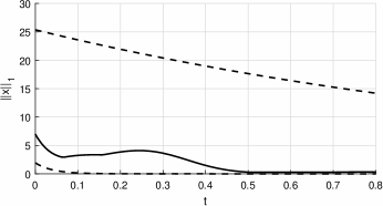
For comparison purpose we calculate the barrier functions for the two vector norms, $\left\lVert\cdot\right\rVert_{1}$ and $\left\lVert\cdot\right\rVert_{2}.$ Meaning the lower and upper barrier function is obvious from Fig.Β 1. We have that

$$\mu_{1}[A(t)]=-11/2+(15/2)(\sin 12t+\left|\cos 12t\right|)\ (=\mu_{\infty}[A(t)])$$
$$\lambda^{+}=\frac{6}{\pi}\int\limits_{0}^{\pi/6}\left[-11/2+(15/2)(\sin 12s+\left|\cos 12s\right|)\right]ds$$

$=-0.7253$ and $\delta^{+}_{U}=1.2872.$ Analogously,

$$\lambda^{-}=\frac{6}{\pi}\int\limits_{0}^{\pi/6}\left[41/2+(15/2)(\sin 12s+\left|\cos 12s\right|)\right]ds$$

$=25.2747,$ and $\delta^{-}_{U}=1.2871.$ For the LN $\mu_{2}$ we analogously obtain:

$$\mu_{2}[A(t)]=\frac{15\sqrt{2}\sqrt{\sin 12t+1}}{2}-13\in[-13,2],$$
$$\lambda^{+}=\frac{6}{\pi}\int\limits_{0}^{\pi/6}\left[\frac{15\,\sqrt{2}\,\sqrt{\sin 12s+1}}{2}-13\right]ds$$

$=-3.4507,$ and $\delta^{+}_{U}=0.9337;$

$$\lambda^{-}=\frac{6}{\pi}\int\limits_{0}^{\pi/6}\left[\frac{15\,\sqrt{2}\,\sqrt{\sin 12s+1}}{2}+13\right]ds$$

$=22.5493,$ and $\delta^{-}_{U}=1.0441.$

Refer to caption
Figure 1: The functions eΞ +​(t)=e∫0tΞΌ1​[A​(s)]​𝑑ssuperscript𝑒superscriptΠ𝑑superscript𝑒superscriptsubscript0𝑑subscriptπœ‡1delimited-[]𝐴𝑠differential-d𝑠e^{\Pi^{+}(t)}=e^{\int\limits_{0}^{t}\mu_{1}[A(s)]ds} with $\mu_{1}[A(t)]=-11/2+(15/2)\big{(}\sin 12t+\left|\cos 12t\right|\big{)}$ (the solid line) and the lower and upper barrier functions $e^{\lambda^{+}t+\delta^{+}_{L}}=e^{-0.7253t-0.0364},$ $e^{\lambda^{+}t+\delta^{+}_{U}}=e^{-0.7253t+1.2872}$ (the dashed lines).
Refer to caption
(a) Simulation for $\left\lVert\cdot\right\rVert_{1}$
Refer to caption
(b) Simulation for $\left\lVert\cdot\right\rVert_{2}$
Figure 2: The solution of (6) with the initial state $x(0)=(-4,\ 3)^{T}$ (the solid line); the bounds for $\left\lVert x(t)\right\rVert_{1}:(|-4|+|3|)e^{-0.7253t+1.2872}$, $(|-4|+|3|)e^{-25.2747t-1.2871}$ (the dashed lines); the bounds for $\left\lVert x(t)\right\rVert_{2}:\sqrt{25}e^{-3.4507t+0.9337}$, $\sqrt{25}e^{-22.5493t-1.0441}$ (the dashed lines).

In this example, the use of the Euclidean vector $\mu_{2}[A(t)]$ provides the better information regarding the position of the FCEs ($=\sigma_{R}$) in the complex-plane as those given by octahedral norm $\mu_{1}[A(t)],$ the vertical strip $\{z\in\mathbb{C}:\,-22.5493\leq\Re\{z\}\leq-3.4507\}_{\mu_{2}}$ and $\{z\in\mathbb{C}:\,-25.2747\leq\Re\{z\}\leq-0.7253\}_{\mu_{1}},$ respectively. The result of simulation is in Fig.Β 2.

II-D Note regarding the robustness of exponentially stable LPTV systems against disturbances

In this section we will analyze the stability properties of the LPTV systems affected by an external disturbance $d(t).$ Let us consider that the unperturbed system $\dot{x}=A(t)x$ is UES. What can we say about the asymptotic behavior of its perturbation $\dot{x}=A(t)x+d(t)?$ This question represents one of the fundamental problems on the field of robust stability. The robustness of the systems’ stability is not usually analyzed together with establishing the sufficient conditions ensuring the stability of some kind for the LTV systems. Among these include, e.Β g., [16, 28, 21, 29, 27]. We have the following result regarding asymptotic behavior of perturbed LPTV systems as $t\to\infty.$

Theorem 3

Let us consider the perturbed LPTV system,

$$\dot{x}=A(t)x+d(t),\quad A(t+T)=A(t),\quad t\geq t_{0}\,(\geq 0),$$ (7)

where $A(\cdot):[0,\infty)\to\mathbb{R}^{n\times n}$ and $d(\cdot):[0,\infty)\to\mathbb{R}^{n}$ are continuous and let

  • A1)

    Ξ +​(t0+T)<0,superscriptΞ subscript𝑑0𝑇0\Pi^{+}(t_{0}+T)<0, that is, the unperturbed system is UES, and

  • A2)

    $\left\lVert d(t)\right\rVert\to 0$ as $t\to\infty.$

Then all solutions of (7) converge to 00 as $t\to\infty$ (not necessarily exponentially).

Proof:

The solution of (7) is given by the Lagrange’s variation of constants formula,

$$x(t)=X(t)X^{-1}(t_{0})x(t_{0})+X(t)\int\limits_{t_{0}}^{t}X^{-1}(\tau)d(\tau)d\tau$$

and so $\left\lVert x(t)\right\rVert$

$$\leq\left\lVert X(t)X^{-1}(t_{0})\right\rVert\left\lVert x(t_{0})\right\rVert+\int\limits_{t_{0}}^{t}\left\lVert X(t)X^{-1}(\tau)\right\rVert\left\lVert d(\tau)\right\rVert d\tau.$$

Using the inequality βˆ₯X​(t)​Xβˆ’1​(Ο„)βˆ₯≀eΞ +​(t0+T)T​(tβˆ’Ο„)​eΞ΄U+βˆ’Ξ΄L+delimited-βˆ₯βˆ₯𝑋𝑑superscript𝑋1𝜏superscript𝑒superscriptΞ subscript𝑑0π‘‡π‘‡π‘‘πœsuperscript𝑒subscriptsuperscriptπ›Ώπ‘ˆsubscriptsuperscript𝛿𝐿\left\lVert X(t)X^{-1}(\tau)\right\rVert\leq e^{\frac{\Pi^{+}(t_{0}+T)}{T}(t-\tau)}e^{\delta^{+}_{U}-\delta^{+}_{L}} from the proof of TheoremΒ 2, we have

βˆ₯x​(t)βˆ₯≀βˆ₯x​(t0)βˆ₯​eΞ +​(t0+T)T​(tβˆ’t0)​eΞ΄U+delimited-βˆ₯βˆ₯π‘₯𝑑delimited-βˆ₯βˆ₯π‘₯subscript𝑑0superscript𝑒superscriptΞ subscript𝑑0𝑇𝑇𝑑subscript𝑑0superscript𝑒subscriptsuperscriptπ›Ώπ‘ˆ\left\lVert x(t)\right\rVert\leq\left\lVert x(t_{0})\right\rVert e^{\frac{\Pi^{+}(t_{0}+T)}{T}(t-t_{0})}e^{\delta^{+}_{U}}
+eΞ΄U+βˆ’Ξ΄L+β€‹βˆ«t0teΞ +​(t0+T)T​(tβˆ’Ο„)​βˆ₯d​(Ο„)βˆ₯​𝑑τsuperscript𝑒subscriptsuperscriptπ›Ώπ‘ˆsubscriptsuperscript𝛿𝐿superscriptsubscriptsubscript𝑑0𝑑superscript𝑒superscriptΞ subscript𝑑0π‘‡π‘‡π‘‘πœdelimited-βˆ₯βˆ₯π‘‘πœdifferential-d𝜏+e^{\delta^{+}_{U}-\delta^{+}_{L}}\int\limits_{t_{0}}^{t}e^{\frac{\Pi^{+}(t_{0}+T)}{T}(t-\tau)}\left\lVert d(\tau)\right\rVert d\tau
=βˆ₯x​(t0)βˆ₯​eΞ +​(t0+T)T​(tβˆ’t0)​eΞ΄U+absentdelimited-βˆ₯βˆ₯π‘₯subscript𝑑0superscript𝑒superscriptΞ subscript𝑑0𝑇𝑇𝑑subscript𝑑0superscript𝑒subscriptsuperscriptπ›Ώπ‘ˆ=\left\lVert x(t_{0})\right\rVert e^{\frac{\Pi^{+}(t_{0}+T)}{T}(t-t_{0})}e^{\delta^{+}_{U}}
+eΞ΄U+βˆ’Ξ΄L+β€‹βˆ«t0teβˆ’Ξ +​(t0+T)T​τ​βˆ₯d​(Ο„)βˆ₯​𝑑τeβˆ’Ξ +​(t0+T)T​t.superscript𝑒subscriptsuperscriptπ›Ώπ‘ˆsubscriptsuperscript𝛿𝐿superscriptsubscriptsubscript𝑑0𝑑superscript𝑒superscriptΞ subscript𝑑0π‘‡π‘‡πœdelimited-βˆ₯βˆ₯π‘‘πœdifferential-d𝜏superscript𝑒superscriptΞ subscript𝑑0𝑇𝑇𝑑+e^{\delta^{+}_{U}-\delta^{+}_{L}}\frac{\int\limits_{t_{0}}^{t}e^{-\frac{\Pi^{+}(t_{0}+T)}{T}\tau}\left\lVert d(\tau)\right\rVert d\tau}{e^{-\frac{\Pi^{+}(t_{0}+T)}{T}t}}.

Applying the L’Hospital rule to the second term we get

limtβ†’βˆžβˆ«t0teβˆ’Ξ +​(t0+T)T​τ​βˆ₯d​(Ο„)βˆ₯​𝑑τeβˆ’Ξ +​(t0+T)T​t=limtβ†’βˆžβˆ’βˆ₯d​(t)βˆ₯Ξ +​(t0+T)/T=0,subscript→𝑑superscriptsubscriptsubscript𝑑0𝑑superscript𝑒superscriptΞ subscript𝑑0π‘‡π‘‡πœdelimited-βˆ₯βˆ₯π‘‘πœdifferential-d𝜏superscript𝑒superscriptΞ subscript𝑑0𝑇𝑇𝑑subscript→𝑑delimited-βˆ₯βˆ₯𝑑𝑑superscriptΞ subscript𝑑0𝑇𝑇0\lim\limits_{t\to\infty}\frac{\int\limits_{t_{0}}^{t}e^{-\frac{\Pi^{+}(t_{0}+T)}{T}\tau}\left\lVert d(\tau)\right\rVert d\tau}{e^{-\frac{\Pi^{+}(t_{0}+T)}{T}t}}=\lim\limits_{t\to\infty}\frac{-\left\lVert d(t)\right\rVert}{\Pi^{+}(t_{0}+T)/T}=0,

and so $\left\lVert x(t)\right\rVert\to 0$ as $t\to\infty.$ ∎

Remark 5

The perturbation $d(t)$ could have been replaced by a perturbation $\tilde{d}(x,t)$ which satisfies $\left\lVert\tilde{d}(x,t)\right\rVert\leq\left\lVert d(t)\right\rVert$ for all $x\in\mathbb{R}^{n}.$ Since this would have introduced no new ideas, we chose to present the notationally simpler case.

The class of allowable disturbances of the form $d(t)$ preserving the convergence to 00 of the solutions for the UES LPTV unperturbed systems is a little wider [25] and contains also the functions that do not vanish at infinity.

Theorem 4

Let the unperturbed system is UES. Then all solutions of perturbed LPTV system $\dot{x}=A(t)x+d(t),$ $A(t+T)=A(t)$ and perturbed LTI system $\dot{x}=Ax+d(t)$ converge to 00 as $t\to\infty$ if and only if

$$\sup\limits_{0\leq\eta\leq 1}\left\lVert\int\limits_{t}^{t+\eta}d(\tau)d\tau\right\rVert\to 0\quad\mathrm{as}\quad t\to\infty.$$ (8)

By [25, CorollaryΒ 4.6], the class of allowable perturbations $d(x,t)$ contains also the functions of the form $D(t)k(x),$ where $D(t)$ is an $n\times n$ bounded matrix on $[0,\infty)$ whose columns satisfy (8) and $k:\mathbb{R}^{n}\to\mathbb{R}^{n}$ is continuous.

III Conclusion

We derived, in TheoremΒ 2, the new criterion for uniform and uniform exponential stability of the linear periodic time-varying (LPTV) systems $\dot{x}=A(t)x,$ $t\geq t_{0},$ $A(t+T)=A(t),$ $T>0$ without direct computing of the Floquet characteristic exponents (FCEs). We have shown that the FCEs lie in the vertical strip $\{z\in\mathbb{C}:-\lambda^{-}\leq\Re\{z\}\leq\lambda^{+}\}$ of the complex-plane. Here $\lambda^{+}=\frac{1}{T}\int\limits_{t_{0}}^{t_{0}+T}\mu[A(s)]ds$ and $\lambda^{-}=\frac{1}{T}\int\limits_{t_{0}}^{t_{0}+T}\mu[-A(s)]ds,$ where $\mu[\cdot]$ denotes the logarithmic norm (LN) of matrix associated with an appropriately chosen vector norm. We also briefly discussed the persistence of the stability properties for the perturbed LPTV systems under the external disturbances $d(t).$ The fundamental advantage of the approach based on the use of LN is the fact that to estimate the norm of state-transition matrix $\Phi(t,\tau)$ for system $\dot{x}=A(t)x$ we do not need to know the fundamental matrix solution and all necessary estimates are based purely on the matrix $A(t)$ entries.

References

  • [1] V.N. Afanas’ev, V.B. Kolmanovskii, and V.R. Nosov, Mathematical Theory of Control Systems Design. Springer, 1996.
  • [2] R.Β Bellman, Stability theory of differential equations, McGraw-Hill Book Company, Inc., 1953.
  • [3] R.W. Brockett, Finite dimensional linear systems, John Wiley & Sons, Inc., 1970.
  • [4] C.Β Chicone, Ordinary Differential Equations with Applications, Springer, New York, 1999.
  • [5] P. Colaneri, Theoretical aspects of continuous-time periodic systems, Annual Reviews in Control 29, 205 -215 (2005).
  • [6] W.A. Coppel, Dichotomies in Stability Theory, Springer-Verlag Berlin Heidelberg, 1978.
  • [7] W.A. Coppel, Stability and Asymptotic Behavior of Differential Equations, D. C. Heath and Company Boston, 1965.
  • [8] J.J. DaCunha, J.M. Davis, A unified Floquet theory for discrete, continuous, and hybrid periodic linear systems, J. Differential Equations 251 2987 -3027 (2011).
  • [9] C.A. Desoer, Slowly varying system $\dot{x}=A(t)x$, IEEE Transactions on Automatic Control, vol.14, 780–781 (1969).
  • [10] C.A. Desoer, H. Haneda, The Measure of a Matrix as a Tool to Analyze Computer Algorithms for Circuit Analysis IEEE Transactions on Circuits Theory 19, 5, 480–486 (1972).
  • [11] C.A. Desoer, M. Vidyasagar, Feedback Systems: Input-output Properties. Society for Industrial and Applied Mathematics, Philadelphia, 2009.
  • [12] W. Gao, Z-P. Jiang, F.L. Lewis, and Y. Wang, Leader-to-Formation Stability of Multi-Agent Systems: An Adaptive Optimal Control Approach, IEEE Transactions on Automatic Control 63, 10, 3581–3587 (2018).
  • [13] G. Garcia, P.L.D. Peres, and S. Tarbouriech, Necessary and sufficient numerical conditions for asymptotic stability of linear time-varying systems, Proceedings of the 47th IEEE Conference on Decision and Control Cancun, Mexico, 5146–5151 (2008).
  • [14] D.A. Harville, Matrix Algebra From a Statistician s Perspective. Springer, New York, 2008.
  • [15] G.-D. Hu, M. Liu, The weighted logarithmic matrix norm and bounds of the matrix exponential, Linear Algebra and its Applications 390, 145 -154 (2004).
  • [16] A. Ilchmann, D.H.Owens, and D. PrΓ€tzel-Wolters, Sufficient conditions for stability of linear time-varying systems, Systems & Control Letters 9, 157–163 (1987).
  • [17] A. Ioannou and J. Sun, Robust Adaptive Control. Prentice-Hall, Upper Saddle River, NJ, 1996.
  • [18] N.A. Izobov, Lyapunov Exponents and Stability, Cambridge Scientific Publishers, Cambridge, 2012.
  • [19] H.H. Rosenbrock, The stability of linear time dependent control systems, Int. Journal Electr. Control, vol.15, 73–80 (1963).
  • [20] W.Β J.Β Rugh, Linear system theory (2nd ed.), Prentice-Hall, Inc., 1996.
  • [21] S. Safavi, U.A. Khan, Asymptotic Stability of LTV Systems With Applications to Distributed Dynamic Fusion, IEEE Transactions on Automatic Control 62(11), 5888–5893 (2017).
  • [22] J.S. Shamma and M. Athans, Guaranteed properties of gain scheduled control for linear parameter-varying plants, Automatica 27(3), 559- 564 (1991).
  • [23] G. SΓΆderlind, The logarithmic norm. History and modern theory, BIT Numerical Mathematics 46, 631- 652 (2006).
  • [24] G. SΓΆderlind, R.M.M. Mattheij, Stability and asymptotic estimates in nonautonomous linear differential systems. SIAM J. Math. Anal. 16, No.Β 1, 69–92 (1985).
  • [25] A. Strauss, and J.A. Yorke, Perturbing uniform asymptotically stable nonlinear systems, Journal of Differential Equations 6, 452 -483 (1969).
  • [26] J.-P. Tian, J. Wang, Some results in Floquet theory, with application to periodic epidemic models, Applicable Analysis 94, 1128–1152 (2015).
  • [27] M.Y. Wu, A note on stability of linear time-varying systems, IEEE Transactions on Automatic Control 19, 162–163 (1974).
  • [28] B. Zhou, On asymptotic stability of linear time-varying systems, Automatica, 68, 266–276 (2016).
  • [29] J.-M. Wang, Explicit Solution and Stability of Linear Time-varying Differential State Space Systems, International Journal of Control, Automation and Systems 15(4), 1553–1560 (2017).