Distributed Integer Balancing under Weight Constraints
in the Presence of Transmission Delays and Packet Drops

Abstract

We consider the distributed weight balancing problem in networks of nodes that are interconnected via directed edges, each of which is able to admit a positive integer weight within a certain interval, captured by individual lower and upper limits. A digraph with positive integer weights on its (directed) edges is weight-balanced if, for each node, the sum of the weights of the incoming edges equals the sum of the weights of the outgoing edges. In this work, we develop a distributed iterative algorithm which solves the integer weight balancing problem in the presence of arbitrary (time-varying and inhomogeneous) time delays that might affect transmissions at particular links. We assume that communication between neighboring nodes is bidirectional, but unreliable since it may be affected from bounded or unbounded delays (packet drops), independently between different links and link directions. We show that, even when communication links are affected from bounded delays or occasional packet drops (but not permanent communication link failures), the proposed distributed algorithm allows the nodes to converge to a set of weight values that solves the integer weight balancing problem, after a finite number of iterations with probability one, as long as the necessary and sufficient circulation conditions on the lower and upper edge weight limits are satisfied. Finally, we provide examples to illustrate the operation and performance of the proposed algorithms.

I INTRODUCTION

A distributed system or network consists of a set of components (nodes) that can share information with neighboring components via connection links (edges), forming a generally directed interconnection topology (digraph). The digraphs that describe the communication and/or physical topology typically prove to be of vital importance for the effectiveness of distributed strategies in performing various tasks [2003:jadbabaie_coordination, 2007:olfati-saber_consensus, 2008:RenBeard, 2018:BOOK_Hadj].

A weighted digraph is a digraph in which each edge is associated with a real or integer value called the edge weight. Similarly, a flow network (also known as a transportation network) is a digraph where each edge receives a flow that typically cannot exceed a given capacity (or, more generally, has to lie within upper and lower limits). A weighted digraph (or flow network) is weight-balanced or balanced if, for each of its nodes, the sum of the weights of the edges outgoing from the node is equal to the sum of the weights of the edges incoming to the node.

The problem we deal with in this paper can be viewed as the problem of weight/flow balancing under integer weight/flow constraints on each edge of a given digraph [2014:RikosHadj], or the problem of producing a feasible circulation in a directed graph with upper and lower flow constraints [1986:Papadimitriou]. Furthermore, it can also be seen as a particular case of the standard network flow problem (see, e.g., [2010:Fulkerson]), where there is a cost associated to the flow on each link, and the objective is to minimize the total cost subject to balancing constraints on the flows.

Weight-balanced digraphs find numerous applications in distributed adaptive control and synchronization in complex networks. Examples of applications where balance plays a key role include modeling of flocking behavior [2003:jadbabaie_coordination], network adaptation strategies based on the use of continuous second order models [2010:DeLellis], prediction of distribution matrices for telephone traffic [1998:Bertsekas], distributed adaptive strategies to tune the coupling weights of a network based on local information of node dynamics [2012:YuDeLellis], and design of cut-balanced networks for consensus seeking systems [2013:Julien_Tsitsiklis]. Weight/flow balance is also closely related to weights/flows that form a doubly stochastic matrix [2012:CortesJournal], which find applications in multicomponent systems (such as sensor networks) where one is interested in distributively averaging measurements at each component. Asymptotic consensus to the real average [1984:Tsitsiklis] or the quantized average [2016:ChamieBasar] of the initial values is guaranteed if the weights used in the linear iteration form a doubly stochastic matrix. In particular, the distributed average consensus problem has received significant attention from the computer science community [1996:Lynch] and the control community [2004:XiaoBoyd] due to its applicability to diverse areas, including multi-agent systems, distributed estimation and tracking [2008:CarliChiusoSchenatoZampieri], and distributed optimization [2010:Nedic]. A review of recent approaches to distributed average consensus (and its applications to various settings) can be found in [2018:BOOK_Hadj].

Recently, quite a few works have dealt with the problem of balancing a strongly connected digraph with either real or integer weights/flows. For example, [2009:Cortes, 2018:BOOK_Hadj, 2014:RikosHadj, 2013:Priolo, RikosHadjDelays_2017] deal with distributed algorithms for weight/flow balancing when the nonnegative weights on each edge are otherwise unconstrained (in terms of the values they admit), [2016:RikosHadj, 2016:HadjAlej] deal with the problem of weight/flow balancing assuming timely and reliable exchange of information between nodes, and [2017:RikosHadj_Allerton] deals with weight/flow balancing when the nonnegative weights on each edge are constrained and admit real values (resulting to asymprotic convergence) in the presence of unreliable communication links.

In this paper, we investigate the problem of integer weight/flow balancing in a multi-component system under a directed interconnection topology, where the flow/weight on each edge consists of lower and upper constraints (in terms of the values it admits) in the presence of bounded delays or unbounded delays (packet drops) in the communication links. We consider a fixed topology (digraph) and we devise a protocol, based on our previous work in [2017:RikosHadj], where each node updates its state by combining the available (possibly delayed) weight information received by its in-neighbors. We establish that the proposed balancing algorithm reaches, after a finite number of steps, a set of weights that form a weight-balanced digraph despite the presence of arbitrary but bounded delays in the communication links. When packet drops (i.e., infinite delays) are present over the communication links, we propose a modified version of the algorithm that is shown to converge to a set of weights that form a balanced graph after a finite number of iterations (with probability one). In both cases, we argue that the proposed algorithm reaches a solution as long as such as set of weights exists.

The remainder of this paper is organized as follows. In Section II the notation used throughout the paper is provided, along with background on graph theory and the problem formulation. In Section III we present the conditions for the existence of a set of integer weights (within the interval constraints) that balance a weighted digraph. In Section IV we present the distributed algorithm which achieves integer weight-balancing in the presence of bounded delays after a finite number of iterations. In Section LABEL:algorithm_packetDr, we analyze the case of unbounded delays (packet drops) in the communication links and we present a distributed algorithm which achieves integer weight-balancing after a finite number of iterations with probability one. Finally, in Section LABEL:results we present simulation results and comparisons, and we conclude in Section LABEL:future with a brief summary and remarks about our future work.

II NOTATION AND BACKGROUND

Matrices are denoted by capital letters. The sets of real, integer, natural and nonnegative integer numbers are denoted by $\mathds{R},\mathds{Z}$, $\mathds{N}$ and $\mathds{N}_{0}$ respectively.

II-A Graph-Theoretic Notions

A distributed system whose components can exchange certain quantities of interest via (possibly directed) links, can conveniently be captured by a digraph (directed graph). A digraph of order $n$ ($n\geq 2$), is defined as $\mathcal{G}_{d}=(\mathcal{V},\mathcal{E})$, where $\mathcal{V}=\{v_{1},v_{2},\dots,v_{n}\}$ is the set of nodes and $\mathcal{E}\subseteq\mathcal{V}\times\mathcal{V}-\{(v_{j},v_{j})$ $|$ $v_{j}\in\mathcal{V}\}$ is the set of edges. A directed edge from node $v_{i}$ to node $v_{j}$ is denoted by $(v_{j},v_{i})\in\mathcal{E}$, and indicates that a nonnegative flow of mass from node $v_{i}$ to node $v_{j}$ is possible. We will refer to the digraph $\mathcal{G}_{d}$ as the topology.

A digraph is called strongly connected if for each pair of vertices $v_{j},v_{i}\in\mathcal{V}$, $v_{j}\neq v_{i}$, there exists a directed path from $v_{i}$ to $v_{j}$, i.e., we can find a sequence of vertices $v_{i}\equiv v_{l_{0}},v_{l_{1}},\dots,v_{l_{t}}\equiv v_{j}$ such that $(v_{l_{\tau+1}},v_{l_{\tau}})\in\mathcal{E}$ for $\tau=0,1,\dots,t-1$. All nodes that can have flows to node $v_{j}$ directly are said to be in-neighbors of node $v_{j}$ while the nodes that receive flows from node $v_{j}$ comprise its out-neighbors. The in- and out-neighbors of node $v_{j}$ are nodes in the set $\mathcal{N}_{j}^{-}=\{v_{i}\in\mathcal{V}\;|\;(v_{j},v_{i})\in\mathcal{E}\}$ and $\mathcal{N}_{j}^{+}=\{v_{l}\in\mathcal{V}\;|\;(v_{l},v_{j})\in\mathcal{E}\}$ respectively, where the cardinality of $\mathcal{N}_{j}^{-}$ is called the in-degree of $v_{j}$ (denoted by $\mathcal{D}_{j}^{-}$) and the cardinality of $\mathcal{N}_{j}^{+}$ is called the out-degree of $v_{j}$ (denoted by $\mathcal{D}_{j}^{+}$). We let $\mathcal{N}_{j}=\mathcal{N}^{+}_{j}\cup\mathcal{N}^{-}_{j}$ denote the neighbors of node $v_{j}$, and $\mathcal{D}_{j}=\mathcal{D}^{+}_{j}+\mathcal{D}^{-}_{j}$ denote the total degree of node $v_{j}$. Also, $\mathcal{E}^{-}_{j}=\{(v_{j},v_{i})\ |\ v_{i}\in\mathcal{N}^{-}_{j}\}$ ($\mathcal{E}^{+}_{j}=\{(v_{l},v_{j})\ |\ v_{l}\in\mathcal{N}^{+}_{j}\}$) denotes the incoming (outgoing) edges to (from) node $v_{j}$. Note that $|\mathcal{E}^{-}_{j}\cup\mathcal{E}^{+}_{j}|=\mathcal{D}^{+}_{j}+\mathcal{D}^{-}_{j}=\mathcal{D}_{j}$, where $\mathcal{D}_{j}$ is the total degree of node $v_{j}$.

We assume that node $v_{j}$ assigns a “unique order” in the set $\{0,1,...,\mathcal{D}_{j}-1\}$ to each of its outgoing and incoming edges. The order of edge $(v_{l},v_{j})$ (or edge ($v_{j}$, $v_{i}$)) is denoted by $P_{lj}$ (or $P_{ji}$) (such that $\{P_{lj}\;|\;v_{l}\in\mathcal{N}^{+}_{j}\}\cup\{P_{ji}\;|\;v_{i}\in\mathcal{N}^{-}_{j}\}=\{0,1,...,\mathcal{D}_{j}-1\}$) and will be used later on as a way of allowing node $v_{j}$ to make changes to its outgoing and incoming edge flows in a predetermined order. Note that the “unique order” is cyclic in the sense that every time a node attempts to change the flows of its incoming/outgoing edges, it continues from the edge it stopped the previous time according to the predetermined order, starting from the beginning if it has changed the values of every incoming and outgoing edge.

We assume that a pair of nodes $v_{j}$ and $v_{i}$ that are connected by an edge in the digraph $\mathcal{G}_{d}$ (i.e., $(v_{j},v_{i})\in\mathcal{E}$ and/or $(v_{i},v_{j})\in\mathcal{E}$) can exchange information among themselves (in both directions). In other words, the communication topology is captured by the undirected graph $\mathcal{G}_{u}=(\mathcal{V},\mathcal{E}_{u})$ that corresponds to the given directed graph $\mathcal{G}_{d}=(\mathcal{V},\mathcal{E})$, where $\mathcal{E}_{u}=\cup_{(v_{j},v_{i})\in\mathcal{E}}\{(v_{j},v_{i}),(v_{i},v_{j})\}$.

II-B Flow/Weight Balancing

Given a digraph $\mathcal{G}_{d}=(\mathcal{V},\mathcal{E})$ we aim to assign positive integer flows $f_{ji}\in\mathds{N}$ to each edge $(v_{j},v_{i})\in\mathcal{E}$. In this paper, these flows will be restricted to lie in an interval $[l_{ji},u_{ji}]$, i.e., $0<l_{ji}\leq f_{ji}\leq u_{ji}$ and $f_{ji}\in\mathds{N}$, for every $(v_{j},v_{i})\in\mathcal{E}$. We will also use matrix notation and denote (respectively) the integer flow, perceived integer flow, lower limit, and upper limit matrices by the $n\times n$ matrices $F=[f_{ji}]$, $F_{p}=[f^{(p)}_{ji}]$, $L=[l_{ji}]$, and $U=[u_{ji}]$, where $F(j,i)=f_{ji}$, $F_{p}(j,i)=f^{(p)}_{ji}$, $L(j,i)=l_{ji}$, $U(j,i)=u_{ji}$, for every $(v_{j},v_{i})\in\mathcal{E}$ (obviously, $f_{ji}=f^{(p)}_{ji}=l_{ji}=u_{ji}=0$ when $(v_{j},v_{i})\notin\mathcal{E}$).

Definition 1.

Given a digraph $\mathcal{G}_{d}=(\mathcal{V},\mathcal{E})$ of order $n$ along with an integer flow assignment $F=[f_{ji}]$, the total in-flow of node $v_{j}$ is defined as $f_{j}^{-}=\sum_{v_{i}\in\mathcal{N}_{j}^{-}}f_{ji}$, the total out-flow of node $v_{j}$ is defined as $f_{j}^{+}=\sum_{v_{l}\in\mathcal{N}_{j}^{+}}f_{lj}$ and the flow balance $b_{j}$ of node $v_{j}$ is $b_{j}=f_{j}^{-}-f_{j}^{+}$.

Definition 2.

Given a digraph $\mathcal{G}_{d}=(\mathcal{V},\mathcal{E})$ of order $n$, along with an integer flow assignment $F=[f_{ji}]$ and a perceived flow assignment $F_{p}=[f^{(p)}_{ji}]$, the total perceived in-flow $f_{j}^{-(p)}$ of node $v_{j}$ is $f_{j}^{-(p)}=\sum_{v_{i}\in\mathcal{N}_{j}^{-}}f^{(p)}_{ji}$ while the perceived flow balance $b^{(p)}_{j}$ of node $v_{j}$ is $b^{(p)}_{j}=f_{j}^{-(p)}-f_{j}^{+}$.

Definition 3.

Given a digraph $\mathcal{G}_{d}=(\mathcal{V},\mathcal{E})$ of order $n$, along with an integer flow assignment $F=[f_{ji}]$, the total imbalance (or absolute imbalance) of digraph $\mathcal{G}_{d}$ is defined as $\varepsilon=\sum_{j=1}^{n}|b_{j}|$, while the perceived total imbalance of digraph $\mathcal{G}_{d}$ is defined as $\varepsilon^{(p)}=\sum_{j=1}^{n}|b^{(p)}_{j}|$. The digraph $\mathcal{G}_{d}$ is called flow-balanced if its total imbalance is zero.

Remark 1.

Note here that the integer flow $f_{lj}$ on edge $(v_{l},v_{j})\in\mathcal{E}$ is assigned by node $v_{j}$. Thus, node $v_{j}$ has access to the true flow $f_{lj}$ of edge $(v_{l},v_{j})$ while node $v_{l}$ has access to a perceived flow $f^{(p)}_{lj}$, which will be equal to $f_{lj}$ if node $v_{j}$ is able to successfully communicate with node $v_{l}$. This means that node $v_{l}$ can only calculate its perceived flow balance $b^{(p)}_{l}$ at each iteration $k$ and it has no access to the total (or perceived total) imbalance of the digraph $\mathcal{G}_{d}$.

II-C Modeling Time Delays and Packet Drops

We assume that a transmission from node $v_{j}$ to node $v_{l}$ at time step $k$ undergoes an a priori unknown delay $\tau^{(j)}_{lj}[k]$ while, we consider both bounded delays and unbounded delays (packet drops). For bounded delays, we assume that $\tau^{(j)}_{lj}[k]$ is an integer that satisfies $0\leq\tau^{(j)}_{lj}[k]\leq\overline{\tau}_{lj}\leq\infty$ where the maximum delay is denoted by $\overline{\tau}=\max_{(v_{l},v_{j})\in\mathcal{E}}\overline{\tau}_{lj}$. In the weight balancing setting we consider that node $v_{j}$ is in charge of assigning the actual flow $f_{lj}[k]$ to each link $(v_{l},v_{j})$, and then transmits to node $v_{l}$ the amount of change $c^{(j)}_{lj}[k]$ it desires at time step $k$. Under the above delay model (which also assumes bidirectional communication), node $v_{l}$ ($v_{j}$) receives the change amount $c^{(j)}_{lj}[k]$ ($c^{(l)}_{lj}[k]$), required by node $v_{j}$ ($v_{l}$) over the actual (perceived) flow $f_{lj}[k]$ ($f^{(p)}_{lj}[k]$), at time step $k+\tau^{(j)}_{lj}[k]$ ($k+\tau_{lj}^{(l)}[k]$).

To handle the case when a transmission from node $v_{j}$ to node $v_{l}$ at time step $k$ undergoes an a priori unknown unbounded delay, we assume that each particular edge may drop packets with some non-total probability. We assume independence between packet drops at different time steps or different links (or even different directions of the same link), so that, we can model a packet drop via a Bernoulli random variable:

$$Pr\{x_{k}(j,i)=m\}=\left\{\begin{array}[]{ll}q_{ji},&\mbox{if $m=0$,}\\ 1-q_{ji},&\mbox{if $m=1$,}\end{array}\right.$$ (1)

where $x_{k}(j,i)=1$ if the transmission from node $v_{i}$ to node $v_{j}$ at time step $k$ is successful.

II-D Problem formulation

We are given a strongly connected digraph $\mathcal{G}_{d}=(\mathcal{V},\mathcal{E})$, as well as lower and upper limits $l_{ji}$ and $u_{ji}$ ($0<l_{ji}\leq u_{ji}$, where $l_{ji},u_{ji}\in\mathds{R}$) on each each edge $(v_{j},v_{i})\in\mathcal{E}$. Considering that link transmissions undergo arbitrary, bounded (or unbounded) delays, we want to develop a distributed algorithm that allows the nodes to iteratively adjust the integer flows on their edges so that they eventually obtain a set of integer flows $\{f_{ji}\;|\;(v_{j},v_{i})\in\mathcal{E}\}$ that satisfy the following:

1. $f_{ji}\in\mathds{N}$ for each edge $(v_{j},v_{i})\in\mathcal{E}$;

2. $l_{ji}\leq f_{ji}\leq u_{ji}$ for each edge $(v_{j},v_{i})\in\mathcal{E}$;

3. $f_{j}^{+}=f_{j}^{-}=f_{j}^{-(p)}$ for each $v_{j}\in\mathcal{V}$.

The distributed algorithm needs to respect the communication constraints imposed by the undirected graph $\mathcal{G}_{u}$ that corresponds to the given directed graph $\mathcal{G}_{d}$. Specifically, the communication topology is captured by the undirected graph $\mathcal{G}_{u}=(\mathcal{V},\mathcal{E}_{u})$ that corresponds to a given directed graph $\mathcal{G}_{d}=(\mathcal{V},\mathcal{E})$, where $\mathcal{E}_{u}=\cup_{(v_{j},v_{i})\in\mathcal{E}}\{(v_{j},v_{i}),(v_{i},v_{j})\}$.

Remark 2.

One of the main differences of the work in this paper with the works in [2010:Cortes, 2009:Cortes, 2014:RikosHadj, 2013:Priolo, 2012:Rikos, RikosHadjDelays_2017] is that the algorithm developed in this paper requires a bidirectional communication topology, whereas most of the aforementioned works assume a communication topology that matches the flow (physical) topology. We should point out that direct application of these earlier algorithms to the problem that is of interest in this paper will generally fail (because flows are restricted to lie within lower and upper limits). Also, note that there are many applications where the physical topology is directed but the communication topology is bidirectional. One such example is the traffic network that was mentioned earlier; it is represented by a digraph, in which unidirectional or bidirectional edges (possibly capacity constrained) capture, respectively, one-way or two-way streets, and where nodes capture intersections. Traffic lights typically sit at these intersections and aim to control traffic flow; even though traffic lights may be constrained in terms of how they divert flow (depending on the constraints of the traffic network), communication between neighboring traffic lights can be bidirectional. In other words, there are two graphs: the directed (physical) graph representing the actual traffic flow over streets/edges and the likely undirected (cyber or communication) graph representing the communication capability between nodes in the graph. In applications like the traffic network mentioned above, the algorithms proposed here are directly applicable. More generally, in many applications, the communication topology may not necessarily match the physical one; in our future work, we plan to enhance the algorithm proposed here to allow for different communication topologies (including the one that matches the physical topology).

III NECESSARY AND SUFFICIENT CONDITIONS: INTEGER CIRCULATION CONDITIONS

When edge weights are restricted to be integers, the theorem below (a variation of the well known circulation conditions) characterizes the necessary and sufficient conditions (e.g., see Theorem $3.1$ in [2010:Fulkerson]) for the existence of a set of integer flows that satisfy interval constraints and balance constraints.

Theorem 1.

Consider a strongly connected digraph $\mathcal{G}_{d}=(\mathcal{V},\mathcal{E})$, with lower and upper bounds $l_{ji}$ and $u_{ji}$ (where $0<l_{ji}\leq u_{ji}$) on each edge $(v_{j},v_{i})\in\mathcal{E}$. The necessary and sufficient conditions for the existence of a set of integer flows $\{f_{ji}\in\mathds{N}\ |\;(v_{j},v_{i})\in\mathcal{E}\}$ that satisfy

1. Interval constraints: $0<l_{ji}\leq f_{ji}\leq u_{ji}$ for each edge $(v_{j},v_{i})\in\mathcal{E}$, and

2. Balance constraints: $f_{j}^{+}=f_{j}^{-}$ for every $v_{j}\in\mathcal{V}$,

are the following:

1. for every $(v_{j},v_{i})\in\mathcal{E}$, we have $\lceil l_{ji}\rceil\leq\lfloor u_{ji}\rfloor,$ and

2. for each $\mathcal{S}$, $\mathcal{S}\subset\mathcal{V}$, we have

   $$\sum_{(v_{j},v_{i})\in\mathcal{E}^{-}_{\mathcal{S}}}\lceil l_{ji}\rceil\leq\sum_{(v_{l},v_{j})\in\mathcal{E}^{+}_{\mathcal{S}}}\lfloor u_{lj}\rfloor\;,$$ (2)

where

$$\mathcal{E}^{-}_{\mathcal{S}} = \{(v_{j},v_{i})\in\mathcal{E}\;|\;v_{j}\in\mathcal{S},\;v_{i}\in\mathcal{V}-\mathcal{S}\}\;,$$ (3)

$$\mathcal{E}^{+}_{\mathcal{S}} = \{(v_{l},v_{j})\in\mathcal{E}\;|\;v_{j}\in\mathcal{S},\;v_{l}\in\mathcal{V}-\mathcal{S}\}\;.$$ (4)

Remark 3.

Note that Theorem 1 effectively requires $\mathcal{G}_{d}$ to be strongly connected or a pure collection of strongly connected sub-digraphs. The necessity of the conditions described in Theorem 1 follows from the conditions in [2010:Fulkerson]: when flows are restricted to be integers, the effective interval of $f_{ji}$ is the interval $[\lceil l_{ji}\rceil,\lfloor u_{ji}\rfloor]$ and clearly has to be non-empty for each $(v_{j},v_{i})\in{\mathcal{V}}$ (condition (i) above).

IV INTEGER FLOW BALANCING ALGORITHM WITH TIME DELAYS

In this section we provide an overview of the distributed flow algorithm operation; the formal description of the algorithm is provided in Algorithm 1. The algorithm is iterative and operates by having, at each iteration, nodes with positive perceived flow balance attempt to change the integer flows on both their incoming and/or outgoing edges so that they become flow balanced. We first describe the distributed iterative algorithm operations and we establish that, if the necessary and sufficient integer circulation conditions in Theorem 1 are satisfied, the algorithm completes after a finite number of iterations.

Initialization. At initialization, each node is aware of the feasible flow interval on each of its incoming and outgoing edges, i.e., node $v_{j}$ is aware of $l_{ji},u_{ji}$ for each $v_{i}\in\mathcal{N}^{-}_{j}$ and $l_{lj},u_{lj}$ for each $v_{l}\in\mathcal{N}^{+}_{j}$. Furthermore, the flows are initialized at the ceiling of the lower bound of the feasible interval, i.e., $f_{ji}[0]=\lceil l_{ji}\rceil$. This initialization is always feasible but not critical and could be any integer value in the feasible flow interval $[l_{ji},u_{ji}]$ (according to Theorem 1 an integer always exists in the interval $[l_{ji},u_{ji}]$). Also, each node $v_{j}$ chooses a unique order $P_{lj}^{(j)}$ and $P_{ji}^{(j)}$ for its outgoing links $(v_{l},v_{j})$ and incoming links $(v_{j},v_{i})$ respectively, such that $\{P_{lj}^{(j)}\;|\;v_{l}\in\mathcal{N}^{+}_{j}\}\cup\{P_{ji}^{(j)}\;|\;v_{i}\in\mathcal{N}^{-}_{j}\}=\{0,1,...,\mathcal{D}_{j}-1\}$.

Iteration. At each iteration $k\geq 0$, node $v_{j}$ is aware of the perceived integer flows on its incoming edges $\{f^{(p)}_{ji}[k]\;|\>v_{i}\in\mathcal{N}^{-}_{j}\}$ and the (actual) flows on its outgoing edges $\{f_{lj}[k]\;|\>v_{l}\in\mathcal{N}^{+}_{j}\}$, which allows it to calculate its perceived flow balance $b^{(p)}_{j}[k]$ according to Definition 2.

A. Selecting Desirable Flows. Each node $v_{j}$ with positive perceived flow balance $b^{(p)}_{j}[k]>0$ attempts to subtract $1$ (one unit of flow) from the flows on its incoming edges $\{f_{ji}[k]\;|\;v_{i}\in\mathcal{N}^{-}_{j}\}$ and add $1$ (one unit of flow) to the flows of its outgoing edges $\{f_{lj}[k]\;|\;v_{l}\in\mathcal{N}^{+}_{j}\}$, one at a time by following the predetermined order (chosen at initialization) in a round-robin fashion, until its perceived flow balance $b^{(p)}_{j}[k+1]$ becomes zero (at least if no other changes are inflicted on the flows). If an outgoing (incoming) edge has reached its max (min) value (according to the feasible interval on that particular edge), then its flow does not change and node $v_{j}$ proceeds in changing the flow of the ensuing edge, according to the predetermined order. Note here that no attempt to change flows is made if node $v_{j}$ has negative or zero perceived flow balance. The next time node $v_{j}$ needs to change the flows of its incoming/outgoing edges, it will continue from the edge it stopped the previous time and cycle through the edge weights in a round-robin fashion according to the ordering chosen at initialization. The desired flow change by node $v_{j}$ on edge $(v_{j},v_{i})\in\mathcal{E}$ at iteration $k$ will be denoted by $c_{ji}^{(j)}[k]$; similarly, the desired flow change by node $v_{j}$ on edge $(v_{l},v_{j})\in\mathcal{E}$ at iteration $k$ will be denoted by $c_{lj}^{(j)}[k]$.

B. Exchanging Desirable Flows. Once each node $v_{j}$ with positive perceived flow balance calculates the desirable flow change for each incoming $\{c^{(j)}_{ji}[k]\;|\;v_{i}\in\mathcal{N}^{-}_{j}\}$ and outgoing $\{c^{(j)}_{lj}[k]\;|\;v_{l}\in\mathcal{N}^{+}_{j}\}$ flow, it does the following steps in sequence:

1) It transmits the desirable flow change $c^{(j)}_{ji}[k]$ ($c^{(j)}_{lj}[k]$) to each in- (out-) neighbor $v_{i}$ ($v_{l}$).

2) It receives the (possibly delayed) desired flow changes $\overline{c}^{(i)}_{ji}[k]$ ($\overline{c}^{(l)}_{lj}[k]$) from each in- (out-) neighbor $v_{i}$ ($v_{l}$). From node $v_{j}$’s perspective, the delayed flow change for link $(v_{l},v_{j})$, $\forall v_{l}\in\mathcal{N}^{+}_{j}$, at time step $k$ is given by

$$\overline{c}^{(l)}_{lj}[k]=\sum_{k_{0}=k-\overline{\tau}}^{k}c^{(l)}_{lj}[k_{0}],\text{ for which }k_{0}+\tau^{(l)}_{lj}[k_{0}]=k,$$ (5)

i.e., $\overline{c}^{(l)}_{lj}[k]$ is the sum of flow changes $c^{(l)}_{lj}$ that were sent from $v_{l}$ and are seen by node $v_{j}$ by time step $k$. If no flow change is received due to time delays, then node $v_{j}$ assumes that $\overline{c}^{(i)}_{ji}[k]=0$ ($\overline{c}^{(l)}_{lj}[k]=0$) for the corresponding incoming (outgoing) edge $(v_{j},v_{i})$ ($(v_{l},v_{j})$).

3) It calculates its new outgoing (perceived incoming) flows $f_{lj}[k+1]=f_{lj}[k]+c_{lj}^{(j)}[k]+\overline{c}_{lj}^{(l)}[k]$ ($f_{ji}^{(p)}[k+1]=f_{ji}^{(p)}[k]+c_{ji}^{(j)}[k]+\overline{c}_{ji}^{(i)}[k]$). Then, the new outgoing (perceived incoming) flows are adjusted so that the new flow is projected onto the feasible interval $[l_{lj},u_{lj}]$ ($[l_{ji},u_{ji}]$) of the corresponding edge. This (along with all the parameters involved) can be seen in Figure 1.

Remark 4.

Since the flow $f_{ji}$ on each edge $(v_{j},v_{i})\in\mathcal{E}$ affects positively the flow balance $b_{j}[k]$ of node $v_{j}$ and negatively the flow balance $b_{i}[k]$ of node $v_{i}$, we need to take into account the possibility that both nodes desire a change on the flow simultaneously. Thus, the proposed algorithm attempts to coordinate the flow change. The challenge, however, is the fact that time delays may occur during transmissions (in either direction) while the nodes are trying to agree on a flow value.

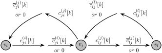
Figure 1: Digraph where nodes exchange their desirable flows in the presence of time delays.

Algorithm 1 Distributed Flow Balancing Algorithm

Input
1) A strongly connected digraph $\mathcal{G}_{d}=(\mathcal{V},\mathcal{E})$ with $n=|\mathcal{V}|$ nodes and $m=|\mathcal{E}|$ edges.
2) $l_{ji},u_{ji}$ for every $(v_{j},v_{i})\in\mathcal{E}$, such that the circulation conditions in Theorem 1 are satisfied.
Initialization
Set $k=0$; each node $v_{j}\in\mathcal{V}$ does:
1) It sets the flows on its perceived incoming and outgoing edge flows as

$$f^{(p)}_{ji}[0]=\lceil l_{ji}\rceil,\ \forall v_{i}\in\mathcal{N}_{j}^{-},$$

$$f_{lj}[0]=\lceil l_{lj}\rceil,\ \forall v_{l}\in\mathcal{N}_{j}^{+}.$$

2) It assigns a unique order to its outgoing and incoming edges as $P_{lj}^{(j)}$, for $v_{l}\in\mathcal{N}_{j}^{+}$ or $P_{ji}^{(j)}$, for $v_{i}\in\mathcal{N}_{j}^{-}$ (such that $\{P_{lj}^{(j)}\ |\ v_{l}\in\mathcal{N}_{j}^{+}\}\cup\{P_{ji}^{(j)}\ |\ v_{i}\in\mathcal{N}_{j}^{-}\}=\{0,1,...,\mathcal{D}_{j}-1\}$).
Iteration
For $k=0,1,2,\dots$, each node $v_{j}\in\mathcal{V}$ does the following:
1) It computes its perceived flow balance as in Definition 2

$$b^{(p)}_{j}[k]=\sum_{v_{i}\in\mathcal{N}_{j}^{-}}f_{ji}^{(p)}[k]-\sum_{v_{l}\in\mathcal{N}_{j}^{+}}f_{lj}[k].$$

2) If $b^{(p)}_{j}[k]>0$, it increases (decreases) by $1$ the integer flows $f_{lj}[k]$ ($f_{ji}^{(p)}[k]$) of its outgoing (incoming) edges $v_{l}\in\mathcal{N}_{j}^{+}$ ($v_{i}\in\mathcal{N}_{j}^{-}$) one at a time, following the predetermined order $P_{lj}^{(j)}$ ($P_{ji}^{(j)}$) until its flow balance becomes zero (if an edge has reached its maximum (minimum) value and it cannot be increased (decreased) further, its flow does not change and node $v_{j}$ proceeds in changing the next one according to the predetermined order). Then, it stores the desired change amount for each outgoing edge as $c_{lj}^{(j)}[k]$ and each incoming edge as $c_{ji}^{(j)}[k]$.
3) If $b^{(p)}_{j}[k]>0$, it transmits the desired flow change $c^{(j)}_{lj}[k]$ ($c^{(j)}_{ji}[k]$) on each outgoing (incoming) edge.
4) It receives the (possibly delayed) desired flow change $\overline{c}^{(l)}_{lj}[k]$ ($\overline{c}^{(i)}_{ji}[k]$) from each outgoing (incoming) edge. [If no flow change is received due to time delays it assumes $\overline{c}^{(l)}_{lj}[k]=0$ ($\overline{c}^{(i)}_{ji}[k]=0$) for the corresponding outgoing (incoming) edge.]
5) It sets its outgoing flows to be

$$f_{lj}[k+1]=f_{lj}[k]+c_{lj}^{(j)}[k]+\overline{c}_{lj}^{(l)}[k],$$

and its new perceived incoming flows to be

$$f_{ji}^{(p)}[k+1]=f_{ji}^{(p)}[k]+c_{ji}^{(j)}[k]+\overline{c}_{ji}^{(i)}[k].$$

6) It adjusts the new outgoing flows according to the corresponding upper and lower weight constraints as

$$f_{lj}[k+1]=\max\{l_{lj},\min\{u_{lj},f_{lj}[k+1]\}\},$$

and its new perceived incoming flows according to the corresponding upper and lower weight constraints as

$$f_{ji}^{(p)}[k+1]=\max\{l_{ji},\min\{u_{ji},f_{ji}^{(p)}[k+1]\}\}.$$

7) It repeats (increases $k$ to $k+1$ and goes back to Step 1).